New relativistic dissipative fluid dynamics from kinetic theory

Abstract

Starting with the relativistic Boltzmann equation where the collision term is generalized to include nonlocal effects via gradients of the phase-space distribution function, and using Grad’s 14-moment approximation for the distribution function, we derive equations for the relativistic dissipative fluid dynamics. We compare them with the corresponding equations obtained in the standard Israel-Stewart and related approaches. Our method generates all the second-order terms that are allowed by symmetry, some of which have been missed by the traditional approaches based on the 14-moment approximation, and the coefficients of other terms are altered. The first-order or Navier-Stokes equations too get modified. Significance of these findings is demonstrated in the framework of one-dimensional scaling expansion of the matter formed in relativistic heavy-ion collisions.

I Introduction

Relativistic fluid dynamics finds applications in cosmology, astrophysics, and the physics of high-energy heavy-ion collisions. In cosmology and certain areas of astrophysics, one needs a fluid dynamics formulation consistent with the General Theory of Relativity Ibanez . On the other hand, a formulation based on the Special Theory of Relativity is quite adequate to treat the evolution of the strongly interacting matter formed in high-energy heavy-ion collisions when it is close to a local thermodynamic equilibrium. The correct formulation of the relativistic dissipative fluid dynamics is far from settled and is currently under intense investigation Baier:2006um ; Baier:2007ix ; Bhattacharyya:2008jc ; Natsuume:2007ty ; El:2008yy ; El:2009vj ; Denicol:2010xn ; Denicol:2012cn .

In applications of fluid dynamics it is natural to first employ the zeroth order (in gradients of the hydrodynamic four-velocity, for example) or ideal fluid dynamics. However, as all fluids are dissipative in nature due to the uncertainty principle Danielewicz:1984ww , the ideal fluid results serve only as a benchmark when dissipative effects become important. The first-order dissipative fluid dynamics or the relativistic Navier-Stokes (NS) theory Landau involves parabolic differential equations and suffers from acausality and instability. The second-order Israel-Stewart (IS) theory Israel:1979wp , with its hyperbolic equations restores causality but may not guarantee stability Huovinen:2008te .

The second-order viscous hydrodynamics has been quite successful in explaining the spectra and azimuthal anisotropy of particles produced in heavy-ion collisions at the Relativistic Heavy Ion Collider (RHIC) Romatschke:2007mq ; Song:2010mg and recently at the Large Hadron Collider (LHC) Luzum:2010ag ; Qiu:2011hf . However, IS theory can lead to unphysical effects such as reheating of the expanding medium Muronga:2003ta and to a negative pressure Martinez:2009mf at large viscosity indicating its breakdown. Furthermore, from comparison to the transport theory it was demonstrated Huovinen:2008te ; El:2008yy that IS approach becomes marginal when the shear viscosity to entropy density ratio $\eta/s\gtrsim 1.5/(4\pi)$. With this motivation, the dissipative hydrodynamic equations were extended El:2009vj to third order, which led to an improved agreement with the kinetic theory even for moderately large values of $\eta/s$.

It is well known that the approach based on the generalized second law of thermodynamics fails to capture all the terms in the evolution equations of the dissipative quantities when compared with similar equations derived from transport theory Baier:2006um . It was pointed out that using directly the definitions of the dissipative currents, instead of the second moment of the Boltzmann equation as in IS theory, one obtains identical equations of motion but with different coefficients Denicol:2010xn . Recently, it has been shown Denicol:2012cn that a generalization of Grad’s 14-moment method Grad results in additional terms in the dissipative equations.

It is important to note that all formulations that employ the Boltzmann equation make a strict assumption of a local collision term in the configuration space Israel:1979wp ; Denicol:2010xn . In other words, within an infinitesimal fluid element containing a large number of particles and extending over many interparticle spacings Landau , the different collisions that increase or decrease the number of particles with a given momentum $p$ are all assumed to occur at the same point $x^{\mu}$. This makes the collision integral a purely local functional of the single-particle phase-space distribution function $f(x,p)$ independent of the derivatives $\partial_{\mu}f(x,p)$. In kinetic theory, $f(x,p)$ is assumed to vary slowly over space-time, i.e., it changes negligibly over the range of interparticle interaction deGroot . However, its variation over the fluid element may not be insignificant; see Fig. 1. Inclusion of the gradients of $f(x,p)$ in the collision term will affect the evolution of dissipative quantities and thus the entire dynamics of the system.

In this Letter, we shall provide a new formal derivation of the dissipative hydrodynamic equations within kinetic theory but using a nonlocal collision term in the Boltzmann equation. We obtain new second-order terms and show that the coefficients of the other terms are altered. These modifications do have a rather strong influence on the evolution of the viscous medium as we shall demonstrate in the case of one-dimensional scaling expansion.

II Nonlocal collision term

Our starting point is the relativistic Boltzmann equation for the evolution of the phase-space distribution function, $p^{\mu}\partial_{\mu}f=C[f]$, where the collision term $C[f]$ is required to be consistent with the energy-momentum and current conservation. Traditionally $C[f]$ is also assumed to be a purely local functional of $f(x,p)$, independent of $\partial_{\mu}f$. This locality assumption is a powerful restriction Israel:1979wp which we relax by including the gradients of $f(x,p)$ in $C[f]$. This necessarily leads to the modified Boltzmann equation

$$p^{\mu}\partial_{\mu}f=C_{m}[f]=C[f]+\partial_{\mu}(A^{\mu}f)+\partial_{\mu}\partial_{\nu}(B^{\mu\nu}f)+\cdots,$$ (1)

where $A^{\mu}$ and $B^{\mu\nu}$ depend on the type of the collisions ($2\leftrightarrow 2,~{}2\leftrightarrow 3,\ldots$).

For instance, for $2\leftrightarrow 2$ elastic collisions,

$$C[f] = \frac{1}{2}\int dp^{\prime}dk\ dk^{\prime}\ W_{pp^{\prime}\to kk^{\prime}}$$ (2)

$$\times(f_{k}f_{k^{\prime}}\tilde{f}_{p}\tilde{f}_{p^{\prime}}-f_{p}f_{p^{\prime}}\tilde{f}_{k}\tilde{f}_{k^{\prime}}),$$

where $W_{pp^{\prime}\to kk^{\prime}}$ is the collisional transition rate, $f_{p}\equiv f(x,p)$ and $\tilde{f}_{p}\equiv 1-rf(x,p)$ with $r=1,-1,0$ for Fermi, Bose, and Boltzmann gas, and $dp=gd{\bf p}/[(2\pi)^{3}\sqrt{{\bf p}^{2}+m^{2}}]$, $g$ and $m$ being the degeneracy factor and particle rest mass. The first and second terms in Eq. (2) refer to the processes $kk^{\prime}\to pp^{\prime}$ and $pp^{\prime}\to kk^{\prime}$, respectively. These processes are traditionally assumed to occur at the same space-time point $x^{\mu}$ with an underlying assumption that $f(x,p)$ is constant not only over the range of interparticle interaction but also over the entire infinitesimal fluid element of size $dR$, which is large compared to the average interparticle separation Landau ; see Fig. 1. Equation (1) together with this crucial assumption has been used to derive the standard second-order dissipative hydrodynamic equations Romatschke:2009im ; Israel:1979wp ; Denicol:2010xn . We, however, emphasize that the space-time points at which the above two kinds of processes occur should be separated by an interval $|\xi^{\mu}|\leq dR$ within the volume $d^{4}R$. It may be noted that the large number of particles within $d^{4}R$ collide among themselves with various separations $\xi^{\mu}$. Further, $\xi^{\mu}$ is independent of the arbitrary point $x^{\mu}$ at which the Boltzmann equation is considered, and is a function of $(p^{\prime},k,k^{\prime})$. Of course, the points $(x^{\mu}-\xi^{\mu})$ must lie within the past light-cone of the point $x^{\mu}$ (i.e., $\xi^{2}>0$ and $\xi^{0}>0$) to ensure that the evolution of $f(x,p)$ in Eq. (1) does not violate causality. With this realistic viewpoint, the second term in Eq. (2) involves $f(x-\xi,p)f(x-\xi,p^{\prime})\tilde{f}(x-\xi,k)\tilde{f}(x-\xi,k^{\prime})$, which on Taylor expansion at $x^{\mu}$ up to second order in $\xi^{\mu}$, results in the modified Boltzmann equation (1) with

$$A^{\mu} = \frac{1}{2}\int dp^{\prime}dk\ dk^{\prime}\ \xi^{\mu}W_{pp^{\prime}\to kk^{\prime}}f_{p^{\prime}}\tilde{f}_{k}\tilde{f}_{k^{\prime}},$$

$$B^{\mu\nu} = -\frac{1}{4}\int dp^{\prime}dk\ dk^{\prime}\ \xi^{\mu}\xi^{\nu}W_{pp^{\prime}\to kk^{\prime}}f_{p^{\prime}}\tilde{f}_{k}\tilde{f}_{k^{\prime}}.$$ (3)

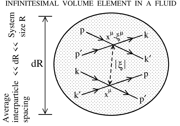
Figure 1: Collisions $kk^{\prime}\to pp^{\prime}$ and $pp^{\prime}\to kk^{\prime}$ occurring at points $x^{\mu}$ and $x^{\mu}-\xi^{\mu}$ within an infinitesimal fluid element of size $dR$, around $x^{\mu}$, containing a large number of particles represented by dots.

In general, for all collision types ($2\leftrightarrow 2,~{}2\leftrightarrow 3,\ldots$), the momentum dependence of the coefficients $A^{\mu}$ and $B^{\mu\nu}$ can be made explicit by expressing them in terms of the available tensors $p^{\mu}$ and the metric $g^{\mu\nu}\equiv{\rm diag}(1,-1,-1,-1)$ as $A^{\mu}=a(x)p^{\mu}$ and $B^{\mu\nu}=b_{1}(x)g^{\mu\nu}+b_{2}(x)p^{\mu}p^{\nu}$, in the spirit of Grad’s 14-moment approximation. Equation (1) forms the basis of our derivation of the second-order dissipative hydrodynamics.

III Hydrodynamic equations

The conserved particle current and the energy-momentum tensor are expressed as deGroot

$$N^{\mu}=\int dp\ p^{\mu}f,~{}~{}T^{\mu\nu}=\int dp\ p^{\mu}p^{\nu}f.$$ (4)

The standard tensor decomposition of the above quantities results in

$$N^{\mu} = nu^{\mu}+n^{\mu},$$

$$T^{\mu\nu} = \epsilon u^{\mu}u^{\nu}-(P+\Pi)\Delta^{\mu\nu}+\pi^{\mu\nu},$$ (5)

where $P,n,\epsilon$ are respectively pressure, number density, energy density, and $\Delta^{\mu\nu}=g^{\mu\nu}-u^{\mu}u^{\nu}$ is the projection operator on the three-space orthogonal to the hydrodynamic four-velocity $u^{\mu}$ defined in the Landau frame: $T^{\mu\nu}u_{\nu}=\epsilon u^{\mu}$. For small departures from equilibrium, $f(x,p)$ can be written as $f=f_{0}+\delta f$. The equilibrium distribution function is defined as $f_{0}=[\exp(\beta u\cdot p-\alpha)+r]^{-1}$ where the inverse temperature $\beta=1/T$ and $\alpha=\beta\mu$ ($\mu$ being the chemical potential) are defined by the equilibrium matching conditions $n\equiv n_{0}$ and $\epsilon\equiv\epsilon_{0}$. The scalar product is defined as $u.p\equiv u_{\mu}p^{\mu}$. The dissipative quantities, viz., the bulk viscous pressure, the particle diffusion current and the shear stress tensor are

$$\Pi = -\frac{\Delta_{\alpha\beta}}{3}\int dp\ p^{\alpha}p^{\beta}\delta f,$$

$$n^{\mu} = \Delta^{\mu\nu}\int dp\ p_{\nu}\delta f,$$

$$\pi^{\mu\nu} = \Delta^{\mu\nu}_{\alpha\beta}\int dp\ p^{\alpha}p^{\beta}\delta f.$$ (6)

Here $\Delta^{\mu\nu}_{\alpha\beta}=[\Delta^{\mu}_{\alpha}\Delta^{\nu}_{\beta}+\Delta^{\mu}_{\beta}\Delta^{\nu}_{\alpha}-(2/3)\Delta^{\mu\nu}\Delta_{\alpha\beta}]/2$ is the traceless symmetric projection operator. Conservation of current, $\partial_{\mu}N^{\mu}=0$ and energy-momentum tensor, $\partial_{\mu}T^{\mu\nu}=0$, yield the fundamental evolution equations for $n$, $\epsilon$ and $u^{\mu}$

$$Dn+n\partial_{\mu}u^{\mu}+\partial_{\mu}n^{\mu} = 0,$$

$$D\epsilon+(\epsilon+P+\Pi)\partial_{\mu}u^{\mu}-\pi^{\mu\nu}\nabla_{(\mu}u_{\nu)} = 0,$$

$$(\epsilon+P+\Pi)Du^{\alpha}-\nabla^{\alpha}(P+\Pi)+\Delta^{\alpha}_{\nu}\partial_{\mu}\pi^{\mu\nu} = 0.$$ (7)

We use the standard notation $A^{(\alpha}B^{\beta)}=(A^{\alpha}B^{\beta}+A^{\beta}B^{\alpha})/2$, $D=u^{\mu}\partial_{\mu}$, and $\nabla^{\alpha}=\Delta^{\mu\alpha}\partial_{\mu}$. For later use we introduce $X^{\langle\mu\rangle}=\Delta^{\mu}_{\nu}X^{\nu}$ and $X^{\langle\mu\nu\rangle}=\Delta^{\mu\nu}_{\alpha\beta}X^{\alpha\beta}$.

Conservation of current and energy-momentum implies vanishing zeroth and first moments of the collision term $C_{m}[f]$ in Eq. (1), i.e., $\int dp\ C_{m}[f]=0=\int dp\ p^{\mu}C_{m}[f]$. Moreover, the arbitrariness in $\xi^{\mu}$ requires that these conditions be satisfied at each order in $\xi^{\mu}$. Retaining terms up to second order in derivatives leads to three constraint equations for the coefficients ($a,b_{1},b_{2}$), namely $\partial_{\mu}a=0$,

$$\partial^{2}\left(b_{1}\langle 1\rangle_{0}\right)+\partial_{\mu}\partial_{\nu}\left(b_{2}\langle p^{\mu}p^{\nu}\rangle_{0}\right) = 0,$$

$$u_{\alpha}\partial_{\mu}\partial_{\nu}\left(b_{2}\langle p^{\mu}p^{\nu}p^{\alpha}\rangle_{0}\right)+u_{\alpha}\partial^{2}\left(b_{1}nu^{\alpha}\right) = 0,$$ (8)

where we define $\langle\cdots\rangle_{0}=\int dp(\cdots)f_{0}$. It is straightforward to show using Eq. (III) that the validity of the second law of thermodynamics, $\partial_{\mu}s^{\mu}\geq 0$, enforces a further constraint $|a|<1$, on the collision term $C_{m}[f]$.

In order to obtain the evolution equations for the dissipative quantities, we follow the approach as described by Denicol-Koide-Rischke (DKR) in Ref. Denicol:2010xn . This approach employs directly the definitions of the dissipative currents in contrast to the IS derivation which uses the second moment of the Boltzmann equation. The comoving derivatives of the dissipative quantities can be written from their definitions, Eq. (III), as

$$\dot{\Pi} = -\frac{\Delta_{\alpha\beta}}{3}\int dp\ p^{\alpha}p^{\beta}\delta\dot{f},$$

$$\dot{n}^{\mu} = \Delta^{\mu\nu}\int dp\ p_{\nu}\delta\dot{f},$$

$$\dot{\pi}^{\mu\nu} = \Delta^{\mu\nu}_{\alpha\beta}\int dp\ p^{\alpha}p^{\beta}\delta\dot{f},$$ (9)

where, $\dot{X}=DX$. Comoving derivative of the nonequilibrium part of the distribution function, $\delta\dot{f}$, can be obtained by writing the Boltzmann equation (1) in the form,

$$\delta\dot{f}=-\dot{f}_{0}-\frac{1}{u.p}p^{\mu}\nabla_{\mu}f+\frac{1}{u.p}C_{m}[f].$$ (10)

To proceed further, we take recourse to Grad’s 14-moment approximation Grad for the single-particle distribution in orthogonal basis Denicol:2010xn

$$f=f_{0}+f_{0}\tilde{f}_{0}\left(\lambda_{\Pi}\Pi+\lambda_{n}n_{\alpha}p^{\alpha}+\lambda_{\pi}\pi_{\alpha\beta}p^{\alpha}p^{\beta}\right).$$ (11)

The coefficients ($\lambda_{\Pi},\lambda_{n},\lambda_{\pi}$) are functions of ($n,\epsilon,\beta,\alpha$). Using Eqs. (III)-(11) and introducing first-order shear tensor $\sigma_{\mu\nu}=\nabla_{\langle\mu}u_{\nu\rangle}$, vorticity $\omega_{\mu\nu}=(\nabla_{\mu}u_{\nu}-\nabla_{\nu}u_{\mu})/2$ and expansion scalar $\theta=\partial\cdot u$, we finally obtain the following evolution equations for the dissipative fluxes defined in Eq. (III):

$$\dot{\Pi}= ~{}-\frac{\Pi}{\tau_{\Pi}^{\prime}}-\beta_{\Pi}^{\prime}\theta-\tau_{\Pi n}^{\prime}n\cdot\dot{u}-l_{\Pi n}^{\prime}\partial\cdot n-\delta_{\Pi\Pi}^{\prime}\Pi\theta$$

$$-\lambda_{\Pi n}^{\prime}n\cdot\nabla\alpha+\lambda_{\Pi\pi}^{\prime}\pi_{\mu\nu}\sigma^{\mu\nu}+\Lambda_{\Pi\dot{u}}\dot{u}\cdot\dot{u}$$

$$+\Lambda_{\Pi\omega}\omega_{\mu\nu}\omega^{\nu\mu}+(8\ {\rm terms}),$$ (12)

$$\dot{n}^{\langle\mu\rangle}= ~{}-\frac{n^{\mu}}{\tau_{n}^{\prime}}+\beta_{n}^{\prime}\nabla^{\mu}\alpha-\lambda_{n\omega}^{\prime}n_{\nu}\omega^{\nu\mu}-\delta_{nn}^{\prime}n^{\mu}\theta$$

$$-l_{n\Pi}^{\prime}\nabla^{\mu}\Pi+l_{n\pi}^{\prime}\Delta^{\mu\nu}\partial_{\gamma}\pi^{\gamma}_{\nu}+\tau_{n\Pi}^{\prime}\Pi\dot{u}^{\mu}$$

$$-\tau_{n\pi}^{\prime}\pi^{\mu\nu}\dot{u}_{\nu}-\lambda_{n\pi}^{\prime}n_{\nu}\pi^{\mu\nu}+\lambda_{n\Pi}^{\prime}\Pi n^{\mu}$$

$$+\Lambda_{n\dot{u}}\omega^{\mu\nu}\dot{u}_{\nu}+\Lambda_{n\omega}\Delta^{\mu}_{\nu}\partial_{\gamma}\omega^{\gamma\nu}+(9\ {\rm terms}),$$ (13)

$$\dot{\pi}^{\langle\mu\nu\rangle}= ~{}-\frac{\pi^{\mu\nu}}{\tau_{\pi}^{\prime}}+2\beta_{\pi}^{\prime}\sigma^{\mu\nu}-\tau_{\pi n}^{\prime}n^{\langle\mu}\dot{u}^{\nu\rangle}+l_{\pi n}^{\prime}\nabla^{\langle\mu}n^{\nu\rangle}$$

$$+2\lambda_{\pi\pi}^{\prime}\pi_{\rho}^{\langle\mu}\omega^{\nu\rangle\rho}+\lambda_{\pi n}^{\prime}n^{\langle\mu}\nabla^{\nu\rangle}\alpha-\tau_{\pi\pi}^{\prime}\pi_{\rho}^{\langle\mu}\sigma^{\nu\rangle\rho}$$

$$-\delta_{\pi\pi}^{\prime}\pi^{\mu\nu}\theta+\Lambda_{\pi\dot{u}}\dot{u}^{\langle\mu}\dot{u}^{\nu\rangle}+\Lambda_{\pi\omega}\omega_{\rho}^{\langle\mu}\omega^{\nu\rangle\rho}$$

$$+\chi_{1}\dot{b}_{2}\pi^{\mu\nu}+\chi_{2}\dot{u}^{\langle\mu}\nabla^{\nu\rangle}b_{2}+\chi_{3}\nabla^{\langle\mu}\nabla^{\nu\rangle}b_{2}.$$ (14)

The “8 terms” (“9 terms”) involve second-order, linear scalar (vector) combinations of derivatives of $b_{1},b_{2}$. All the terms in the above equations are inequivalent, i.e., none can be expressed as a combination of others via equations of motion Bhattacharyya:2012ex . All the coefficients in Eqs. (12)-(14) are obtained as functions of hydrodynamic variables. For example, some of the transport coefficients related to shear are

$$\tau_{\pi}^{\prime}=\; \beta_{\dot{\pi}}\tau_{\pi},~{}~{}~{}\beta_{\pi}^{\prime}=\tilde{a}\beta_{\pi}/\beta_{\dot{\pi}},$$

$$\beta_{\dot{\pi}}=\; \tilde{a}+\frac{b_{2}}{3\eta\tilde{a}}\left[\langle(u.p)^{3}\rangle_{0}-m^{2}n\right],$$

$$\beta_{\pi}=\; \frac{4}{5}P+\frac{1}{15}(\epsilon-3P)-\frac{m^{4}}{15}\left<(u.p)^{-2}\right>_{0},$$ (15)

where ${\tilde{a}}=(1-a)$. The rest of the coefficients will be given in Amaresh_paper2 .

Retaining only the first-order terms in Eqs. (12)-(14), and using DKR values of bulk viscosity $\zeta$, thermal conductivity $\kappa$ and shear viscosity $\eta$, we get the modified first-order equations for bulk pressure $\Pi=-\tau_{\Pi}^{\prime}\beta_{\Pi}^{\prime}\theta=-\tilde{a}\zeta\theta$, heat current $n^{\mu}=\beta_{n}^{\prime}\tau_{n}^{\prime}\nabla^{\mu}\alpha$ and shear stress tensor $\pi^{\mu\nu}=2\tau_{\pi}^{\prime}\beta_{\pi}^{\prime}\sigma^{\mu\nu}=2\tilde{a}\tau_{\pi}\beta_{\pi}\sigma^{\mu\nu}=2\eta{\tilde{a}}\sigma^{\mu\nu}$. Thus the nonlocal collision term modifies even the first-order dissipative equations. This constitutes one of the main results in the present study.

If $a,\ b_{1}$ and $b_{2}$ are all set to zero, Eqs. (12)-(14) reduce to those obtained by DKR Denicol:2010xn with the same coefficients. Otherwise coefficients of all the terms occurring in the DKR equations get modified. Furthermore, our derivation results in new terms, for instance those with coefficients $\Lambda_{k\dot{u}}$, $\Lambda_{k\omega}$, ($k=\Pi,n,\pi$), which are absent in Denicol:2010xn as well as in the standard Israel-Stewart approach Israel:1979wp . Hence these terms have also been missed so far in the numerical studies of heavy-ion collisions in the hydrodynamic framework Romatschke:2007mq ; Song:2007ux ; Luzum:2010ag . Indeed Eqs. (12)-(14) contain all possible second-order terms allowed by symmetry considerations Bhattacharyya:2012ex . This is a consequence of the nonlocality of the collision term $C_{m}[f]$. However, we note that a generalization of the 14-moment approximation is also able to generate all these terms as shown recently in Ref. Denicol:2012cn .

Figure 2: Time evolution of (a) temperature, shear pressure, inverse Reynolds number and parameters ($b_{1},\ b_{2}$) normalized to their initial values, and (b) anisotropy parameter $P_{L}/P_{T}$. Initial values are $\tau_{0}=0.9$ fm/c, $T_{0}=360$ MeV, $\eta/s=0.16$, $\pi_{0}=4\eta/(3\tau_{0})$. Units of $b_{2}$ are GeV^-2. The curve labelled DKR is obtained by setting $a=b_{1}=b_{2}=0$ in Eqs. (16) and (IV).

IV Numerical results

To demonstrate the numerical significance of the new dissipative equations derived here, we consider evolution of a massless Boltzmann gas, with equation of state $\epsilon=3P$, at vanishing net baryon number density in the Bjorken model Bjorken:1982qr . The new terms, namely $\dot{u}\cdot\dot{u}$, $\omega_{\mu\nu}\omega^{\nu\mu}$, $\omega^{\mu\nu}\dot{u}_{\nu}$, $\Delta^{\mu}_{\nu}\partial_{\gamma}\omega^{\gamma\nu}$, $\dot{u}^{\langle\mu}\dot{u}^{\nu\rangle}$ and $\omega_{\rho}^{\langle\mu}\omega^{\nu\rangle\rho}$ containing acceleration and vorticity do not contribute in this case. However, they are expected to play an important role in the full 3D viscous hydrodynamics.

In terms of the coordinates ($\tau,x,y,\eta$) where $\tau=\sqrt{t^{2}-z^{2}}$ and $\eta=\tanh^{-1}(z/t)$, the initial four-velocity becomes $u^{\mu}=(1,0,0,0)$. In this scenario $\Pi=0=n^{\mu}$ and the equation for $\pi\equiv-\tau^{2}\pi^{\eta\eta}$ reduces to

$$\frac{\pi}{\tau_{\pi}}+\beta_{\dot{\pi}}\frac{d\pi}{d\tau}=\beta_{\pi}\frac{4}{3\tau}-\lambda\frac{\pi}{\tau}-\psi\pi\frac{db_{2}}{d\tau},$$ (16)

where the coefficients are

$$\beta_{\dot{\pi}}\! = \!\tilde{a}+\frac{b_{2}(\epsilon+P)}{\tilde{a}\beta\eta},~{}~{}\beta_{\pi}=\frac{4}{5}\tilde{a}P,~{}~{}\psi=\frac{9(\epsilon+P)}{5\tilde{a}\beta\eta},$$

$$\lambda\! = \!\frac{38}{21}\tilde{a}-\left(\frac{b_{1}\beta}{5}-\frac{8b_{2}}{7\beta}\right)\frac{\epsilon+P}{\tilde{a}\eta}.$$ (17)

For comparison we quote the IS results Israel:1979wp : $\beta_{\pi}=2P/3,~{}\lambda=2$. The coupled differential equations (III), (III) and (16) are solved simultaneously for a variety of initial conditions: temperature $T=360$ or 500 MeV corresponding to typical RHIC and LHC energies, and shear pressure $\pi=0$ or $\pi=\pi_{\rm NS}=4\eta/(3\tau_{0})$ corresponding to isotropic and anisotropic pressure configurations. Since the nonlocal effects embodied in the Taylor expansion (1) are not large, the initial $a,~{}b_{1},~{}b_{2}$ are so constrained that the corrections to first-order and second-order terms remain small; recall also the additional constraints $|a|<1$ and Eq. (III).

Figure 3: Time evolution of $P_{L}/P_{T}$ in IS Israel:1979wp , DKR ($a=b_{1}=b_{2}=0$), and the present work, for isotropic initial pressure configuration $(\pi_{0}=0)$. The scaling $(\eta/s)_{\rm IS}=9/10(\eta/s)$ ensures that all the results are compared at the same cross section Denicol:2010xn .

Figure 2(a) illustrates the evolution of these quantities for a choice of initial conditions. $T$ decreases monotonically to the crossover temperature $~{}170$ MeV at time $\tau\simeq 10$ fm/c, which is consistent with the expected lifetime of quark-gluon plasma. Parameter $a$ is constant whereas $b_{1}$ and $b_{2}$ vary smoothly and tend to zero at large times indicating reduced but still significant presence of nonlocal effects in the collision term at late times. This is also evident in Fig. 2(b) where the pressure anisotropy $P_{L}/P_{T}=(P-\pi)/(P+\pi/2)$ shows marked deviation from IS, controlled mainly by $a$. At late times $P_{L}/P_{T}$ is largely unaffected by the choice of initial values of $b_{1},~{}b_{2}$. Although the shear pressure $\pi$ vanishes rapidly indicating approach to ideal fluid dynamics, the $P_{L}/P_{T}$ is far from unity. Faster isotropization for initial $a>0$ may be attributed to a smaller effective shear viscosity $(1-a)\eta$ in the modified NS equation, and conversely. Figure 2(b) also indicates the convergence of the Taylor expansion that led to Eq. (1).

Figure 3 shows the evolution of $P_{L}/P_{T}$ for isotropic initial pressure configuration, at various $\eta/s$ for the LHC energy regime. Compared to IS, DKR leads to larger pressure anisotropy. Further, with small initial corrections ($10$% to first-order and $\simeq 20$% to the second-order terms) due to $a,\ b_{1},\ b_{2}$, the nonlocal hydrodynamics (solid lines) exhibits appreciable deviation from the (local) DKR theory. The above results clearly demonstrate the importance of the nonlocal effects, which should be incorporated in transport calculations as well. Comparison of nonlocal hydrodynamics to nonlocal transport theory would be illuminating.

In a realistic 2+1 or 3+1 D calculation, one has to choose the thermalization time and the freeze-out temperature together with suitable initial conditions for hydrodynamic velocity, energy density, shear pressure as well as for the nonlocal coefficients $a,~{}b_{1},~{}b_{2}$ to fit $dN/d\eta$ and $p_{T}$ spectra of hadrons, and then predict, for example, the anisotropic flow $v_{n}$ for a given $\eta/s$. Nonlocal effects (especially via $a$) will affect the extraction of $\eta/s$ from fits to the measured $v_{n}$. It may also be noted that although (local) viscous hydrodynamics explains the gross features of $\pi^{-}$ and $K^{-}$ spectra for the (0-5)% most central Pb-Pb collisions at $\sqrt{s_{NN}}=2.76$ TeV, it strongly disagrees with the measured $\bar{p}$ spectrum Floris:2011ru . Further the constituent quark number scaling violation has been observed in the $v_{2}$ and $v_{3}$ data for $\bar{p}$, at this LHC energy Krzewicki:2011ee . The above discrepancies may be attributed partly to the nonlocal effects which can have different implications for two- and three-particle correlations and thus affect the meson and baryon spectra differently.

V Summary

To summarize, we have presented a new derivation of the relativistic dissipative hydrodynamic equations by introducing a nonlocal generalization of the collision term in the Boltzmann equation. The first-order and second-order equations are modified: new terms occur and coefficients of others are altered. While it is well known that the derivation based on the generalized second law of thermodynamics misses some terms in the second-order equations, we have shown that the standard derivation based on kinetic theory and 14-moment approximation also misses other terms. The method presented here is able to generate all possible terms to a given order that are allowed by symmetry. It can also be extended to derive third-order hydrodynamic equations.

- (1) J.M. Ibáñez, in Current Trends in Relativistic Astrophysics: Theoretical, Numerical, Observational, Vol. 617, Lecture Notes in Physics, (Springer, Berlin, 2003). L. Fernández-Jambrina and L.M. González-Romero (eds.).
- (2) R. Baier, P. Romatschke and U. A. Wiedemann, Phys. Rev. C 73 (2006) 064903.
- (3) R. Baier, P. Romatschke, D. T. Son, A. O. Starinets and M. A. Stephanov, JHEP 0804 (2008) 100.
- (4) S. Bhattacharyya, V. E. Hubeny, S. Minwalla and M. Rangamani, JHEP 0802 (2008) 045.
- (5) M. Natsuume and T. Okamura, Phys. Rev. D 77 (2008) 066014 [Erratum-ibid. D 78 (2008) 089902].
- (6) A. El, A. Muronga, Z. Xu and C. Greiner, Phys. Rev. C 79 (2009) 044914.
- (7) A. El, Z. Xu and C. Greiner, Phys. Rev. C 81 (2010) 041901.
- (8) G. S. Denicol, T. Koide and D. H. Rischke, Phys. Rev. Lett. 105 (2010) 162501.
- (9) G. S. Denicol, H. Niemi, E. Molnar and D. H. Rischke, Phys. Rev. D 85 (2012) 114047.
- (10) P. Danielewicz and M. Gyulassy, Phys. Rev. D 31 (1985) 53.
- (11) L.D. Landau and E.M. Lifshitz, Fluid Mechanics (Butterworth-Heinemann, Oxford, 1987), page 1.
- (12) W. Israel and J. M. Stewart, Annals Phys. 118 (1979) 341.
- (13) P. Huovinen and D. Molnar, Phys. Rev. C 79 (2009) 014906.
- (14) P. Romatschke and U. Romatschke, Phys. Rev. Lett. 99 (2007) 172301.
- (15) H. Song, S. A. Bass, U. Heinz, T. Hirano and C. Shen, Phys. Rev. Lett. 106 (2011) 192301.
- (16) M. Luzum, Phys. Rev. C 83 (2011) 044911.
- (17) Z. Qiu, C. Shen and U. W. Heinz, Phys. Lett. B 707 (2012) 151.
- (18) A. Muronga, Phys. Rev. C 69 (2004) 034903.
- (19) M. Martinez and M. Strickland, Phys. Rev. C 79 (2009) 044903.
- (20) H. Grad, Comm. Pure Appl. Math. 2 (1949) 331.
- (21) S.R. de Groot, W.A. van Leeuwen, and Ch.G. van Weert, Relativistic Kinetic Theory — Principles and Applications (North-Holland, Amsterdam, 1980).
- (22) P. Romatschke, Int. J. Mod. Phys. E 19 (2010) 1.
- (23) S. Bhattacharyya, JHEP 1207 (2012) 104.
- (24) A. Jaiswal, R.S. Bhalerao and S. Pal, (in preparation).
- (25) H. Song and U. W. Heinz, Phys. Rev. C 77 (2008) 064901.
- (26) J. D. Bjorken, Phys. Rev. D 27 (1983) 140.
- (27) M. Floris, J. Phys. G 38 (2011) 124025.
- (28) M. Krzewicki for ALICE Collaboration, J. Phys. G 38 (2011) 124047.