A novel code for numerical 3-D MHD studies of CME expansion

Zusammenfassung

A recent third-order, essentially non-oscillatory central scheme to advance the equations of single-fluid magnetohydrodynamics (MHD) in time has been implemented into a new numerical code. This code operates on a 3-D Cartesian, non-staggered grid, and is able to handle shock-like gradients without producing spurious oscillations.
To demonstrate the suitability of our code for the simulation of coronal mass ejections (CMEs) and similar heliospheric transients, we present selected results from test cases and perform studies of the solar wind expansion during phases of minimum solar activity. We can demonstrate convergence of the system into a stable Parker-like steady state for both hydrodynamic and MHD winds. The model is subsequently applied to expansion studies of CME-like plasma bubbles, and their evolution is monitored until a stationary state similar to the initial one is achieved. In spite of the model’s (current) simplicity, we can confirm the CME’s nearly self-similar evolution close to the Sun, thus highlighting the importance of detailed modelling especially at small heliospheric radii.
Additionally, alternative methods to implement boundary conditions at the coronal base, as well as strategies to ensure a solenoidal magnetic field, are discussed and evaluated.

Coronal mass ejections (CMEs) moved into the focus of several research activities during recent years. Besides a variety of observational data resulting from SOHO (Pick et al., 2006), SMEI (Webb et al., 2006), and, very recently, STEREO (Vourlidas et al., 2007), significant progress has also been achieved with the numerical modelling of CMEs, see, e.g., the reviews by Aschwanden et al. (2006) and Forbes et al. (2006). The motivation for the various activities is at least fourfold. First, CMEs are amongst the main mediators of the influence of the Sun on the inner heliosphere, particularly on the Earth and its environment, where they significantly co-determine the space weather conditions. There is, in view of ever advancing technology that is increasingly sensitive — if not vulnerable — to space weather effects, strong interest in an understanding of the latter. An even stronger driver of research activities is provided with the recognition that space weather phenomena offer valuable opportunities to study many aspects of plasma astrophysics in great detail (Scherer et al., 2005; Bothmer and Daglis, 2006; Schwenn, 2006). Second, as a consequence of the shocks driven by CMEs, they serve as particle accelerators that do not only contribute to space weather effects, but can be used to study the actual acceleration processes (Reames, 1999; Mewaldt et al., 2005; Li et al., 2005), which are expected to occur in other astrophysical systems as well (Eichler, 2006). Third, with the recent launch of the two-spacecraft mission STEREO (Kaiser, 2005), the full three-dimensional structure of CMEs can be observed both remotely and in-situ for the first time. First results have already been reported by, e.g., Howard and Tappin (2008) and Vourlidas et al. (2007). And, fourth, the magnetohydrodynamic (MHD) modelling of CMEs provides an excellent testbed for numerical codes. Although not strongly motivated by CME physics, this is actually one of the main drivers of model development, as is manifest with numerous approaches documented in the literature. These various approaches can be ordered into three groups. There is (i) principal modelling that is either analytical and/or based on symmetry assumptions (e.g., Titov and Démoulin, 1999; Roussev et al., 2003; Schmidt and Cargill, 2003; Jacobs et al., 2005), (ii) local modelling limited to the extended corona, i.e. a few tens of solar radii (e.g., Mikić and Linker, 1994), and (iii) global modelling covering the inner heliosphere from the solar surface out to 1 AU and beyond (e.g., Manchester et al., 2004; Odstrčil et al., 2005; Tóth et al., 2005; Riley et al., 2006).
Despite these intensified efforts and activity regarding the study of CMEs, there remains both a number of unsolved problems and various modelling deficiencies. For example, the acceleration and heating processes of the plasma near the coronal base are — even nearly 50 years after the ’discovery’ of the solar wind — still not known (Cranmer et al., 2007), and there is also no agreement on the processes that actually initiate CMEs (Forbes et al., 2006). Also, their propagation and evolution in size and shape is by far not fully understood in all detail, and neither is their interaction with the background solar wind (Jacobs et al., 2007), with other CMEs (Gopalswamy et al., 2001), and with planetary magnetospheres (e.g., Groth et al., 2000; Ip and Kopp, 2002). Regarding the model formulations underlying the numerical simulation of CMEs, particularly the (non-thermal) heating of the plasma is mostly treated in a rather simplified manner via ad-hoc heating functions (e.g., Groth et al., 2000; Manchester et al., 2004), variable adiabatic indices $\gamma=\gamma({\bf r})$ (e.g., Lugaz et al., 2007), or phenomenological heating functions (e.g., Usmanov et al., 2000), for a discussion see Fichtner et al. (2008).
With the intention to address several of the above-mentioned problems, we have applied our recently developed CWENO-based MHD code (Kleimann et al., 2004), which primordially originated from that by Grauer and Marliani (2000), to the CME expansion problem. To our knowledge, this is the first published paper describing the application of a CWENO-based numerical code to an MHD problem related to space physics.
In the following, we describe the model (Sect. 1) and its numerical realization (Sect. 2 to 4), present results of analyses of both the propagation of individual and the interaction of two CMEs, and suggest a possible connection of our findings to observations (Sect. 5).

1 Governing equations

Choosing the normalization constants summarized in Tab. 1, the set of MHD equations for mass density $\rho$, flow velocity ${\bf u}$, magnetic field strength ${\bf B}$, and gas pressure $p$ reads (in dimensionless form):

$$\partial_{t}\rho+\nabla\cdot(\rho\ \vec{u}) = 0$$ (1)

$$\partial_{t}(\rho\ \vec{u})+\nabla\cdot\left[\rho\ \vec{u}\vec{u}\right.$$

$$\left.+(p+\|\vec{B}\|^{2}/2)\ \hat{{\mathbf{I}}}-\vec{B}\vec{B}\right] = \rho\ \vec{g}$$ (2)

$$\partial_{t}\vec{B}+\nabla\cdot\left(\vec{u}\vec{B}-\vec{B}\vec{u}\right) = 0$$ (3)

$$\partial_{t}e+\nabla\cdot\left[(e+p+\|\vec{B}\|^{2}/2)\ \vec{u}\right.$$

$$\left.-(\vec{u}\cdot\vec{B})\vec{B}\right] = \rho\ (Q+\vec{u}\cdot\vec{g})$$ (4)

where

$$\vec{g} = -\Gamma/r^{2}\ \vec{e}_{r}\quad\mbox{and}$$ (5)

$$e = \frac{\rho\ \|\vec{u}\|^{2}}{2}+\frac{\|\vec{B}\|^{2}}{2}+\left\{\begin{array}[]{ccl}p/(\gamma-1)&:&\gamma\neq 1\\ 0&:&\gamma=1\end{array}\right.$$ (8)

respectively denote gravity (with

$$\Gamma:=(GM_{\odot})/(R_{\odot}c_{\rm s}^{2})=11.49$$ (9)

in normalized units, cf. Tab. 1), and the total energy density of a plasma with adiabatic exponent $\gamma$. Throughout this paper, $\|\cdot\|$ is used to denote the norm of a vector (i.e. $\|\vec{X}\|\equiv\sqrt{\vec{X}\cdot\vec{X}}$ for any vector $\vec{X}$), and the symbol $\hat{\bf I}$ in Eq. (2) denotes the unit tensor (i.e. $(\hat{\mathbf{I}})_{ij}=\delta_{ij}$).

Tabelle 1: Normalization constants used for Eqs. (1–4). $M_{\odot}$, $R_{\odot}$, $k_{\rm B}$, $m_{\rm p}$, $\mu_{0}$, and $c_{\rm s}$ denote the solar mass, the solar radius, the Boltzmann constant, the proton rest mass, the electrical permeability of free space, and the isothermal sound speed, respectively.

Quantity	Normalization
(solar) mass	$M_{\odot}=$	$2.0\times 10^{30}\ {\rm kg}$
length	$L_{0}:=R_{\odot}=$	$7.0\times 10^{8}\ {\rm m}$
temperature $T$	$T_{0}:=$	$1.0\times 10^{6}\ {\rm K}$
number density $n\equiv\rho/m_{\rm p}$	$n_{0}:=$	$1.0\times 10^{14}\ {\rm m^{-3}}$
plasma pressure $p$	$2\ n_{0}\ k_{\rm B}\ T_{0}=$	$2.8\times 10^{-3}\ {\rm Pa}$
velocity $u$	$c_{\rm s}:=\sqrt{2\ k_{\rm B}\ T_{0}/m_{\rm p}}=$	$1.3\times 10^{5}\ {\rm m\ s^{-1}}$
time $t$	$L_{0}/c_{\rm s}=$	$5.5\times 10^{3}\ {\rm s}$
energy density $e$	$m_{\rm p}\ n_{0}\ (c_{\rm s})^{2}=$	$2.8\times 10^{-3}\ {\rm J\ m^{-3}}$
mag. induction $B$	$c_{\rm s}\ \sqrt{\mu_{0}\ m_{\rm p}\ n_{0}}=$	$4.2\times 10^{-5}\ {\rm T}$
heating rate $Q$	$(c_{\rm s})^{3}/L_{0}=$	$3.0\times 10^{6}\ {\rm W\ kg^{-1}}$
(CME) mass $M_{\rm cme}$	$m_{\rm p}\ n_{0}\ (L_{0})^{3}=$	$5.7\times 10^{13}$ kg

A Parker-like solution for the solar wind is per construction isothermal, i. e. $\gamma=1$, resulting in an adiabatic cooling for $\gamma>1$. In reality, the decrease in temperature $T\equiv p/\rho$ due to this adiabatic cooling of the expanding plasma is compensated by processes such as reconnective energy release and Alfvénic wave heating. A realistic inclusion of such effects, while certainly desirable, is beyond the scope of this first approach, and, thus, reserved for future refinements of our model. As an alternative, we employ an ad hoc heating function

$$Q=T_{\rm c}\ \alpha(r)\ (\nabla\cdot\vec{u})$$ (10)

with a prescribed heating profile $\alpha(r)$ and a target temperature $T_{\rm c}$. To derive the form of Eq. (10), we first seek the heating function $Q_{\rm iso}$ which maintains a constant temperature $T_{\rm c}$ everywhere, irrespectively of $\gamma$. This is done by inserting the corresponding isothermal equation of state

$$p=T_{\rm c}\ \rho$$ (11)

into the MHD equations (1–4) and solving them analytically for $Q$, which yields

$$Q_{\rm iso}\equiv Q|_{T=T_{\rm c}}=(\nabla\cdot\vec{u})\ T_{\rm c}\ .$$ (12)

Therefore, local heating (or cooling) at any heliocentric radius $r_{\rm h}$ is conveniently achieved by choosing $\alpha(r_{\rm h})>1$ (or $\alpha(r_{\rm h})<1$) in Eq. (10). Test runs demonstrating the validity of this method have been carried out by Kleimann (2005).

2 Numerical implementation

2.1 Algorithm

In order to integrate Eqs. (1–4) forward in time, we employ a 3-D variant (Kleimann et al., 2004) of a recent semi-discrete Central weighted essentially non-oscillatory (CWENO) scheme by Kurganov and Levy (2000) with third-order Runge-Kutta time stepping. Notable advantages of CWENO include its third-order accuracy in smooth regions (which automatically becomes second order near strong gradients to minimize spurious oscillations) and an easy generalization to multi-dimensional systems of equations due to the fact that no (exact or approximate) Riemann solver is needed. The CWENO scheme thus allows simultaneously to achieve high shock resolution comparable with the best shock capturing schemes and high order convergence in smooth regions dominated by plasma waves. Although this scheme is not strictly total variation diminishing (TVD), simulations by Levy et al. (2000) do indicate an upper bound for the total variation of their solutions. Moreover, Havlík and Liska (2006) use a set of astrophysically relevant test cases to compare the performance of several methods for ideal MHD and stress CWENO’s superior accuracy.

2.2 Example test case: Alfvén wings

Various elementary tests of our implementation have been completed successfully (Kleimann et al., 2004), such as advection in one and two dimensions (also for propagation directions inclined at angles $0<\nu<\pi/2$ to the coordinate surfaces), shock tubes with and without magnetic field inclusion, etc.

While those standard tests will not be reproduced here, one rather advanced test setting, which is also of astrophysical relevance involving so-called Älfvén wingsïs worth being mentioned. While the the finite extent of the wave-generating obstacle does not allow for an exact analytical solution, the usefulness of this simple but meaningful test problem stems from the fact that it incorporates several types of MHD waves (Alfvén and slow/ fast magnetosonic), the expansion speed and characteristics of which can be verified quantitatively with theoretical expectations to ensure proper implementation of the relevant physics. As shown by Drell et al. (1965), the movement of a conductive obstacle (e.g. a satellite or small planet) through a homogeneous fluid with a perpendicular magnetic field will generate standing MHD waves in the $(\vec{u},\vec{B})$ plane called Alfvén wings. This phenomenon plays a major role for the interaction of the moon Io with the Jovian magnetosphere (Neubauer, 1980; Linker et al., 1988), and also for artificial satellites in the magnetosphere of Earth, see e. g. Kopp and Schröer (1998) and references therein.
The corresponding numerical test case, which works well both in 2-D and 3-D, involves an initially homogeneous flow $\vec{u}=u_{0}\ \vec{e}_{x}$ of constant density, which is combined with a perpendicular, equally homogeneous magnetic field ${\bf B}=B_{0}\ {\bf e}_{z}$. A solid, spherical obstacle is then implemented by performing an artificial deceleration

$$\begin{array}[]{rl}\vec{u}(\vec{r},t)\leftarrow\vec{u}(\vec{r},t)&\times\left[1-{\rm min}(t,1)\right]\\ &\times\left[1-\tanh(4\ {\rm max}(\|\vec{r}\|-1,0))\right]\end{array}$$ (13)

after each time step, such that for $t\geq 1$, the flow will vanish within $\|\vec{r}\|\leq 1$. Figures 1 and 2 illustrate the emanating wing structure. Direction and speed of propagation agree well with their respective theoretical expectations.

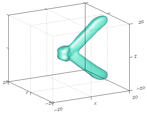
Abbildung 1: 3-D structure of a pair of Alfvén wings, illustrated as an isocontour plot of absolute velocity.

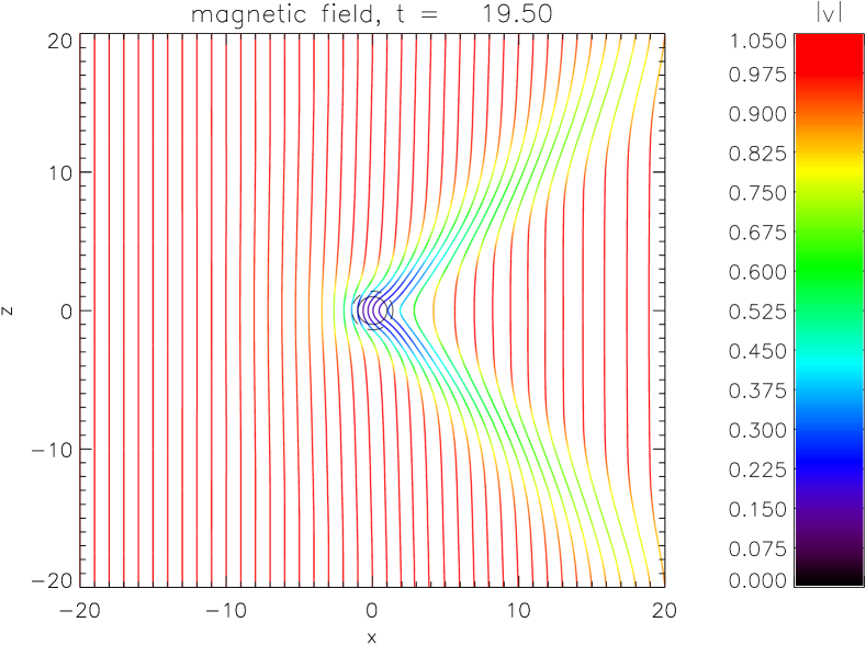
Abbildung 2: Selected magnetic field lines in the $(\vec{u},\vec{B})$ plane, with color denoting flow velocity in normalized units. The flow is incident from the left. Since sound speed and Alfvén speed are both unity, the wings emanate in a tailward $45\degree$ wedge when viewed in the obstacle’s rest frame. The central circle marks the spherical volume inside of which deceleration according to Eq. (13) is applied.

2.3 Choice of coordinates

At first sight, the Sun’s obviously spherical shape would suggest the use of spherical coordinates $[r,\vartheta,\varphi]$, especially since the radial convergence of lines of constant $\vartheta,\varphi$ entails the additional benefit of increased spatial resolution near the Sun’s surface. On the other hand, the Courant-Friedrichs-Lewy (CFL) criterion of numerical validity and stability (Courant et al., 1928), which requires the “velocity” $\Delta x/\Delta t$ to be greater than the maximum physical propagation velocity, imposes a limit on the time step $\Delta t$ based on the cell size $\Delta x$. The very choice of a coordinate system with varying grid cell sizes, together with the requirement that the time step be uniform on the entire grid, thus implies that $\Delta t$ will be set by the $\Delta x$ of the grid’s smallest cell. For spherical coordinates, this means that the increased resolution at small $r$, however welcomed for physical reasons, would force $\Delta t$ to be much lower than what the CFL criterion would require for most parts of the computational domain. This ’problem of small time steps’ is avoided by using Cartesian coordinates, which have equal cell spacing everywhere and thus do not waste computing time on the larger cells. Even worse is the problem of coordinate singularities at the poles $\vartheta\in\{0,\pi\}$, which require delicate numerical treatment. For these reasons, we opt for Cartesian coordinates $[x,y,z]$, for which numerics are faster, simpler (esp. with respect to multi-dimensional extension), and more stable. This is especially true since our CWENO code is built within a framework that allows for Cartesian Adaptive Mesh Refinement (AMR, see (Kleimann et al., 2004)). This is of high interest for more detailed studies of, e.g., the inner structure of a CME. While AMR can, in principle, be used with spherical coordinates, its advantage is over-compensated by the fact that the convergence of grid spacing implies unacceptably low CFL numbers. (Note also that since CMEs generally do not exhibit any clear spatial symmetry, the use of non-Cartesian coordinates is not expected to entail any particular advantages for their description.)

2.4 Divergence cleaning

Like many other algorithms, CWENO does not exactly conserve the solenoidality condition $\nabla\cdot{\bf B}=0$ for the magnetic field, and a correction scheme becomes mandatory to avoid unphysical artifacts. From the wealth of existing schemes (for an overview see, e. g., Tóth (2000)), we have evaluated the performance of the Generalized Lagrange Multiplier (GLM) approach by Dedner et al. (2002) against a classical projection scheme (see Sect. 2.4.2).

2.4.1 The GLM scheme

The GLM scheme solves an additional equation

$$\partial_{t}\Psi+(v_{\rm f})^{2}\ \nabla\cdot\vec{B}=-(v_{\rm f}/\lambda)\ \Psi$$ (14)

for a position- and time-dependent Lagrange multiplier $\Psi$, and adds a term $-\nabla\Psi$ to the right hand side of Eq. (3). This procedure causes $\Psi$ (and hence $\nabla\cdot\vec{B}$) to be damped with decay constant $\tau_{\rm d}:=\lambda/v_{\rm f}$, while at the same time advection of $\Psi$ towards the boundary of the computational volume occurs at the highest permissible speed $v_{\rm f}$ (chosen to equal the global maximum of the fast magnetosonic speed in this case). Following Dedner et al. (2002), a value of 0.18 is used for the second constant $\lambda$.
The main advantage of this method is that Eq. (14) already possesses the correct conservative form, allowing for direct treatment with CWENO. In particular, physical conservation laws are not affected in any way.
Figure 3 compares the performance of the two methods for a standard run. The obviously inferior performance of GLM can be explained by the fact that within a spherical layer ${\cal L}$ around the inner (solar) boundary, the boundary procedure described in section 4.1 entails an averaging of the inner boundary value $\vec{B}_{\rm in}$ and the newly computed outer solution $\vec{B}_{\rm out}$ via

$$\vec{B}_{\rm avg}:=f\vec{B}_{\rm in}+(1-f)\vec{B}_{\rm out}$$ (15)

for some function $f:{\cal L}\mapsto[0,1]$, which is bound to introduce a marked violation of the divergence constraint due to the first term of

$$\nabla\cdot\vec{B}_{\rm avg}=\nabla f\cdot\left(\vec{B}_{\rm in}-\vec{B}_{\rm out}\right)-f\ \nabla\cdot\vec{B}_{\rm out}$$ (16)

being clearly non-zero. This divergence-laden field is then advected outwards by the wind flow, thus causing the magnetic field to quickly become non-solenoidal in the outer region as well. (This behavior becomes particularly evident in the left plot of Fig. 3.)
Since the resulting magnitude of $\nabla\cdot\vec{B}$ in the non-solenoidal interface layer is inversely proportional to the layer’s thickness, the problem cannot be avoided by choosing a different matching method (i. e. a different matching function $r\mapsto f(r)$). Note that this line of reasoning includes the case of doing no averaging at all: This simply corresponds to the limiting case $f=f_{\rm step}$, where

$$f_{\rm step}:\vec{r}\mapsto\left\{\begin{array}[]{rcl}1&:&\|\vec{r}\|\leq 1\\ 0&:&\|\vec{r}\|>1\end{array}\right.\ .$$ (17)

Since this non-solenoidal layer is actively re-created every time the newly computed outer solution is connected to the inner boundary, we may conclude that a suitable divergence cleaning procedure must kill the divergence immediately afterwards in one step (as the projection scheme does), rather than only damping/ transporting it away on somewhat longer timescales (GLM).
We must therefore conclude that for investigations of this kind, the presence of an inner inflow boundary is, at least, difficult and may, in some cases, even preclude the use of the GLM scheme for divergence cleaning. (Note however, that the applicability of GLM to other settings lacking such an internal boundary remains unimpeded by this finding.)

2.4.2 The projection scheme

The so-called ’projection method’ was originally developed by Chorin (1967) for simulations of inviscid flow, and later applied in the context of MHD simulations by Brackbill and Barnes (1980). It solves the Poisson equation

$$\nabla^{2}\Phi=\nabla\cdot\vec{B}$$ (18)

for $\Phi$ and then subtracts $\nabla\Phi$ from $\vec{B}$ to ensure $\nabla\cdot\vec{B}=0$. While numerically expensive, it is able to reduce divergence errors down to machine accuracy, and will therefore be used in all simulations presented here.

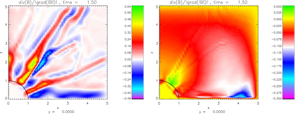
Abbildung 3: Normalized divergence error $\kappa:=(\nabla\cdot\vec{B})/\|\nabla\sqrt{\vec{B}\cdot\vec{B}}\|$ in the (poloidal) $(x,z)$ plane for a standard solar wind run at time $t=1.5$ without correction (left) and using GLM (right). The improvement is substantial but still insufficient due to massive divergence values introduced at the inner boundary (unit circle around the origin). The projection scheme achieves $\kappa\sim 10^{-6}$ (not shown). Note the different color scales.

3 Boundary and initial conditions

3.1 Types of boundaries

The computational volume consists of a brick-shaped region of space covering $100\times 70\times 50$ cells in the $x$, $y$, and $z$ direction, respectively. Each cell is a cube with a side length of typically $\Delta x=\Delta y=\Delta z=0.1$, implying a coverage of $[5,7,10]\ R_{\odot}$ of real space. (We note that this relatively coarse resolution was chosen deliberately do demonstrate the excellent symmetry-maintaining properties of the employed scheme, see also Fig. 5 of Sect. 4.2. Higher spatial resolution, however desirable for the study of fine-scale structures, would tend to diminish the magnitude of numerical artifacts by which the scheme’s performance could be judged, thereby hampering the usefulness of this demonstration.) The Sun’s center is located at the origin, with the dipolar axis pointing into the positive $z$ direction. The computational domain is surrounded by two layers of ’ghost cells’, whose values are updated after each time step either from symmetry considerations (for ’mirror’ boundaries intersecting the origin), or use of outflowing boundary conditions (at the actual ’outer’ boundaries).
The solar surface, which is represented by a sphere of unit radius located inside the computational volume, obviously does not coincide with any of the Cartesian coordinate surfaces, and therefore requires special treatment, which is discussed in detail in Sect. 4.1 and 4.2. This inner boundary is particularly delicate since it constitutes the surface from which the solar wind emanates, such that numerical artifacts imposed by an imperfect treatment of this boundary will be quickly advected through the entire domain.

3.2 Initial conditions

The generic setup for quiet-Sun solar wind simulations is as follows: At $t=0$, the simulation is initialized with a radially symmetric wind flow $\vec{u}(\vec{r})=u(r)\ \vec{e}_{r}$ with

$$u(r)=\frac{u_{\rm m}}{2r_{\rm m}-3}\times\left\{\begin{array}[]{ccl}0&:&r<1\\ (r-1)^{2}&:&1\leq r\leq 2\\ 2r-3&:&r>2\end{array}\right.$$ (19)

such that a super-sonic value ${u_{\rm m}}$ is reached at the innermost boundary point, $r_{\rm m}$. This is done to ensure that the initial velocity at the outer boundary is as small as possible to allow large time steps $\Delta t$, while at the same time being large enough to prevent numerical boundary artifacts from being transported inwards.
The density scales as $\rho(r)\propto 1/r^{3}$, and the temperature is equal to a constant $T_{c}$. The initial magnetic field is implemented using

$$\vec{B}|_{t=0}=\nabla\times\left(\frac{F(r)}{r}\sin\vartheta\ \vec{e}_{\varphi}\right)$$ (20)

where $F(r)=P_{0}/r$ yields a dipole of strength $P_{0}$ that is aligned with the $z$ axis.
Since the projection scheme described in Sect. 2.4.2 will operate on the entire grid, the singularity of Eq. (20) at $r=0$ must be avoided. This is achieved by choosing a suitably matched polynomial for $F(r)$ inside some small sphere around the origin. (Note that the radius of this sphere must be chosen at least several grid cell sizes smaller than unity to prevent the non-zero current density associated with $F(r)\neq P_{0}/r$ from causing unphysical Lorentz force accelerations just outside the $r=1$ boundary.)

4 Numerical treatment of the solar surface boundary

4.1 The interpolation method

The inner (solar surface) boundary, which is just the sphere ${\cal S}:=\{\vec{r}|\ \|\vec{r}\|=1\}$, obviously does not coincide with any of the Cartesian coordinate planes, which brings up the question of how these boundary conditions are best represented on the grid. Simple-minded attempts, such as keeping cell values inside the Sun fixed and integrating only those outside, have been tried but were shown to result in block-like artifacts at small radii (essentially tracing the envelope of the set of grid cells considered ’inside’) where the problem’s symmetry would stipulate spherical contours. While these artifacts would of course diminish as spatial resolution is increased, it seems vital to obtain a high degree of symmetry-keeping already at this relatively coarse resolution, especially in view of the high numerical costs associated with increasing the number of grid cells in a 3-D simulation.
After several possibilities have been tried, the following procedure was adopted:

1. At initialization, all grid points which are located outside ${\cal S}$ but have at least one of their $3^{3}-1=26$ neighbors inside ${\cal S}$ are stored in a list ${\cal I}$ of ’interface points’. (The set neighbors of a cell $\vec{r}_{ijk}$ is defined as the set of cells $\vec{r}_{i^{\prime}j^{\prime}k^{\prime}}$ with $|i-i^{\prime}|,|j-j^{\prime}|,|k-k^{\prime}|\in\{0,1\}$ excluding $\vec{r}_{ijk}$ itself.)

2. After each time step (which only advances grid points outside ${\cal S}$ in time), a weighted average for each variable $w\in\{\rho,\rho u_{x},\rho u_{y},\rho u_{z},B_{x},B_{y},B_{z},e\}$ is computed for each $\vec{r}_{I}\in{\cal I}$ via

   $$\bar{w}_{I}=\left(\sum_{\alpha}(L_{I\alpha})^{-1}\ w(\vec{r}_{\alpha}^{\prime})\right)\left/\left(\sum_{\alpha}(L_{I\alpha})^{-1}\right)\right.$$ (21)

   with

   $$\vec{r}_{\alpha}^{\prime}=\left\{\begin{array}[]{ccc}\vec{r}_{\alpha}&:&\mbox{$r_{\alpha}$ outside of ${\cal S}$}\\ \overline{\vec{r}_{I}\ \vec{r}_{\alpha}}\ \cap\ {\cal S}&:&\mbox{$\!\!\!r_{\alpha}$ inside of ${\cal S}$}\end{array}\right.$$ (22)

   and $L_{I\alpha}:=\|\vec{r}_{I}-\vec{r}_{\alpha}^{\prime}\|$, where the sums in Eq. (21) are taken over all neighbors of $\vec{r}_{I}$. The choice of weights $\propto(L_{I\alpha})^{-1}$ ensures that for $\|{\bf r}_{I}\|\rightarrow 1$, $\bar{w}_{I}$ smoothly tends to the appropriate boundary value. Figure 4 serves to illustrate the situation.
   When the above procedure is applied to the Cartesian components of vectors such as $\vec{u}$ and $\vec{B}$, it will usually destroy any possibly existing symmetry of these vector fields (e. g., if $\vec{u}$ is purely radial, the averaged $\bar{\vec{u}}$ vectors will slightly deviate from the radial direction). In order to preserve such symmetries, all Cartesian vector components entering the averaging process of Eq. (21) are first rotated until they are parallel to $\vec{r}_{I}$ before the averaging takes place, thus ensuring that the symmetry is preserved.

3. In order to guarantee that the newly computed grid values for ${\cal I}$ are independent of the ordering within that list, all computed averages are first stored in a separate field. Only when all the $\bar{w}_{I}$ are known will they be copied onto the actual grid.

Note that step 1 is executed only once, while steps 2 and 3 are called after each integration time step.
The above procedure gives the best results when applied to a scalar field that varies approximately linear in space. Near the solar surface, however, strong radial gradients of density are present. For this reason, it has been found to be advantageous to artificially reduce the density gradient in Eq. (21) by multiplying $\rho(\vec{r}_{\alpha}^{\prime})$ with $\|\vec{r}_{\alpha}^{\prime}\|^{3...4}$ before averaging, and consequently dividing $\bar{\rho_{I}}$ by $\|\vec{r}_{I}\|^{3...4}$ afterwards.

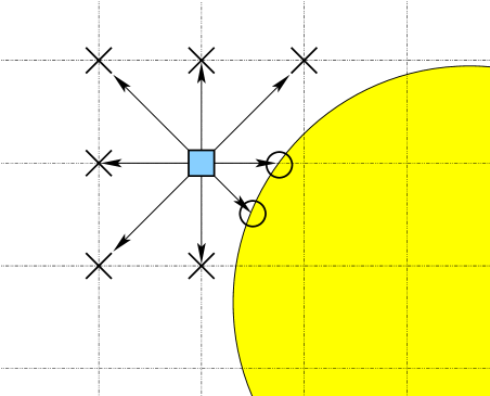
Abbildung 4: 2-D analog of the averaging procedure. At each grid point $\vec{r}_{I}\in{\cal I}$ (shaded central box), a weighted average is computed from time-advanced values taken at neighbors outside ${\cal S}$ (crosses), and boundary values taken in the direction of neighbors inside ${\cal S}$ (circles). The factors $L_{I\alpha}$ entering into Eq. (21) are equivalent to the length of arrows in the diagram.

4.2 Velocity extrapolation versus fixed boundary

The averaging procedure of Sect. 4.1 keeps all quantities fixed on ${\cal S}$. However, if solar wind configurations such as the Parker wind solution (Parker, 1958) are to be reproduced, it seems questionable to apply this procedure to the velocity, since the requirement that $r\mapsto\|\vec{u}(r)\|$ must pass through a critical (sonic) point completely determines the solution topology, and thus eliminates the freedom to prescribe a fixed (Dirichlet) boundary value at $r=1$.
Different possibilities are conceivable to handle this problem:

1. Allow the velocity near ${\cal S}$ to adjust freely by radial inward extrapolation of the time-advanced solution (Keppens and Goedbloed, 2000), or

2. enforce a fixed value for $\vec{u}$ on ${\cal S}$ in spite of the above problem, and accepting that (hopefully small) inaccuracies will be introduced at small radii (Manchester et al., 2004).

While the second alternative is just what the above averaging procedure does, the first option, while being straightforward in spherical coordinates, is clearly non-trivial to implement on the present Cartesian grid.
In analogy to the averaging scheme used for the other variables, the adopted procedure (which replaces the procedure of Sect. 4.1 for $\vec{u}$) is as follows:

1. Prior to initialization, a list ${\cal A}$ of all grid points $\vec{r}_{A}$ with $1\leq\|\vec{r}_{A}\|\leq 0.5$ is set up and sorted by decreasing $\|\vec{r}_{A}\|$ (such that the outermost points will be processed first).

2. For each $\vec{r}_{A}\in{\cal A}$, a sub-list of grid points $\vec{r}_{A,i}$ is created, such that

   • $\|\vec{r}_{A}\|<\|\vec{r}_{A,i}\|$  and

   • $\|\vec{r}_{A}-\vec{r}_{A,i}\|<r_{0}$  (with $r_{0}\approx(2...3)\ \Delta x$).

   In other words, the sub-list for $\vec{r}_{A}$ contains grid points close to $\vec{r}_{A}$ which are located at larger radii than $\vec{r}_{A}$ itself. (Note again that steps 1 and 2 are executed only once.)

3. After each time step, the radial mass flux

   $$f_{A,i}:=(\rho\vec{u})_{A,i}\cdot\vec{r}_{A,i}\ \|\vec{r}_{A,i}\|$$ (23)

   is computed from the sub-list at each $\vec{r}_{A}$, and a least-squares fit of the linear function $g_{A}:r\mapsto c_{0,A}+c_{1,A}\ r$ is used to find the mass flux at $\vec{r}_{A}$ (which is then given by $g_{A}(\|\vec{r}_{A}\|)=c_{0,A}+c_{1,A}\|\vec{r}_{A}\|$). Finally, the corresponding radial momentum is immediately afterwards written to the grid, such that its value is available to the extrapolation at the next point in the list.

Figure 5 shows a comparison of both methods for the (unmagnetized) Parker wind case. The interpolation method’s superior performance is in the range of a few percent only and has to be gauged against its increased computational effort. Consequently, all of the simulations presented here use the Dirichlet method. (We note, however, that this may not always be appropriate when different parameter ranges are used. For instance, a higher base temperature $T_{c}$ will move the sonic point sunwards, leading to a higher flow velocity at the solar surface, and a presumably larger discrepancy to the zero-velocity condition.)

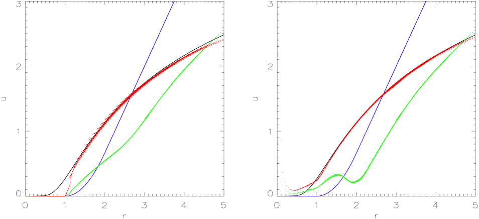
Abbildung 5: Comparison of two possible methods to impose a boundary condition for $\vec{u}$ at the inner boundary $r=1$: Dirichlet boundary condition (left) enforcing $\vec{u}|_{r=1}=\vec{0}$ versus inward extrapolation (right). Both diagrams show scatter plots of absolute velocity $\|\vec{u}\|$ versus heliocentric radius for all $40^{3}$ grid points as the system converges towards the isothermal Parker wind solution (black solid curve). Colors are used to denote the moment of initialization ($t=0$, blue), an intermediate step ($t=1$, green), and the situation after the stationary equilibrium has been reached ($t=8$, red). Since all grid points are shown, the scatter at a given radius can be seen as a measure of the simulation’s spurious departure from radial symmetry.

5 Solar wind and CME simulations

5.1 Creating equilibrium wind solutions

For the initialization of our CME expansion studies, we first seek a well-defined MHD equilibrium resembling a ’quiet’ (i.e. stationary) setting during solar minimum. While this is of course not strictly required for such studies, it is nevertheless vital for the interpretation of the obtained results, since only then can structures like CMEs be clearly disentangled from the dynamics of the background flow.
For magnetized, isothermal ($\gamma=1$) winds, the system starts from the initial conditions of Sect. 3.2 and then quickly (within a few sound crossing times) settles into a stable equilibrium similar to the one depicted in the first frame of Fig. 6. At a distance of 5 $R_{\odot}$ from the origin, the outflow velocity in $x$ direction differs from that at the polar field line by a factor of about

$$\frac{\|{\bf u}(5,0,0)\|}{\|{\bf u}(0,0,5)\|}=\frac{1.26\ c_{\rm s}}{3.13\ c_{\rm s}}\approx\frac{160\ \mbox{km/s}}{400\ \mbox{km/s}}=0.4\ ,$$

which is due to the retaining force of the closed magnetic field lines in the equatorial region, and reminiscent of the speed difference between the fast and slow solar wind. Examples of non-isothermal hydrodynamical runs integrating the full energy equation (4) with the heating source term (10) can be found in (Kleimann, 2005).
It is noteworthy that essential features of the quiet inner heliosphere, such as a latitudinal dependence of outflow velocities resembling the fast and slow solar wind and the poleward transition from closed magnetic field lines (which span a static ’dead zone’) below about $40\degree$ of latitude to an open, more radial field, are self-consistently reproduced by our model. In particular, it was found to be unnecessary to invoke the method of latitude-dependent inner boundary conditions used by other authors (Keppens and Goedbloed, 2000; Manchester et al., 2004) to reproduce this dichotomy: The magnetic dipole strength $P_{0}$ proved fully sufficient to control the latitudinal extent of the closed-field helmet zone. As can be intuitively expected, a stronger B field at the surface will tend to conserve its arch-shaped closed structure, while in the limit $P_{0}\rightarrow 0$, all field lines will be stretched out radially by the flow, and spherical symmetry is recovered. The choice of $P_{0}=4$ results in the intermediate case with an open/ closed transition near $\pm 40\degree$ of solar latitude.

5.2 Initialization of CME onset

The present investigation focuses on the aspect of CME propagation, rather than on their actual nascency. Therefore, a simplifying approach similar to the one already employed by Groth et al. (2000) and Keppens and Goedbloed (2000) will be used. This approach is based on a time-dependent boundary condition at the solar surface, generating a transient, isothermal increase in density (and thus in pressure). If chosen sufficiently strong, this density excess is able to tear open the equatorial helmet streamer, causing the detachment of the excess matter as a rapidly expanding bubble.
In order to initiate an eruption in the time interval

$${\cal T}:=[t_{\rm cme},t_{\rm cme}+\tau_{\rm cme}]$$ (24)

an additional, localized mass flux $\rho_{\rm add}\ \vec{u}_{\rm add}$ with

$$\begin{array}[]{rcl}\rho_{\rm add}(\vec{r},t)|_{r=1}&=&\rho_{\rm cme}(\vec{r},t)\\ \vec{u}_{\rm add}(\vec{r},t)|_{r=1}&=&u_{\rm cme}\ \vec{e}_{r}\end{array}$$ (25)

is released at a pre-defined location on the solar surface (implying $\|\vec{r}\|=1$ for the remainder of this section). Without loss of generality, let the center of the eruption region be in the plane $\varphi=0$, such that its location is just

$$\vec{r}_{\rm cme}:=\left(\begin{array}[]{c}x_{\rm cme}\\ y_{\rm cme}\\ z_{\rm cme}\end{array}\right)=\left(\begin{array}[]{c}\sin\vartheta_{\rm cme}\\ 0\\ \cos\vartheta_{\rm cme}\end{array}\right)\ .$$ (26)

For fixed time $t$, the value of $\rho_{\rm cme}(\vec{r},t)$ should only depend on the angular distance

$$\alpha(\vec{r},\vec{r}_{\rm cme})=\arccos(\vec{r}\cdot\vec{r}_{\rm cme})$$ (27)

between $\vec{r}$ and $\vec{r}_{\rm cme}$, such that $\rho_{\rm cme}(\vec{r},t)$ possesses axial symmetry with respect to the $\vec{r}_{\rm cme}$ axis. Following Keppens and Goedbloed (2000), we employ the function

$$\rho_{\rm cme}(\vec{r},t):=\left\{\begin{array}[]{ccl}\displaystyle f_{0}\ E(\vec{r},t)&:&t\in{\cal T}\wedge\alpha\leq\delta_{\rm cme}\\ &&\\ 0&:&\mbox{else}\end{array}\right.$$ (28)

with

$$E(\vec{r},t):=\sin^{2}\left(\pi\frac{t-t_{\rm cme}}{\tau_{\rm cme}}\right)\ \cos^{2}\left(\frac{\pi}{2}\frac{\alpha(\vec{r},\vec{r}_{\rm cme})}{\delta_{\rm cme}}\right)$$ (29)

which connects smoothly to the undisturbed state in both space and time. Here $2\delta_{\rm cme}$ denotes the angular diameter of the circular eruption region $\Omega_{\rm cme}$, which is defined as the region where $\rho_{\rm cme}({\bf r},t)$ gives a non-zero contribution according to Eq. (28), and which thus covers a total solid angle

$$\omega_{\rm cme}:=\int\limits_{0}^{\delta_{\rm cme}}2\pi\sin\alpha\ {\rm d}\alpha=2\pi\left[1-\cos(\delta_{\rm cme})\right]$$ (30)

on the Sun’s surface. The total mass released by the CME’s eruption can be estimated as

$$M_{\rm cme} := \int\limits_{\cal T}\int\limits_{\Omega_{\rm cme}}\rho_{\rm cme}(\vec{r},t)\ u_{\rm cme}\ {\rm d}\omega\ {\rm d}t$$

$$= f_{0}\ u_{\rm cme}\ \tau_{\rm cme}\ \frac{\pi}{2}\frac{2(\delta_{\rm cme})^{2}-\pi^{2}(1-\cos\delta_{\rm cme})}{(\delta_{\rm cme})^{2}-\pi^{2}},$$

with $\omega$ being the solid angle. For $\delta_{\rm cme}=30\degree=\pi/6$, this translates to physical units as

$$M_{\rm cme,phys.}\approx\frac{f_{0}\ u_{\rm cme}\ \tau_{\rm cme}}{16}\times 10^{14}\ {\rm kg}\ ,$$ (32)

a typical value for a strong CME.

5.3 CME expansion runs

CME expansion runs have been carried out at various combinations of CME strength, heliographic latitude, dipolar field strength, etc. We first describe typical runs involving only a single CME, while the case of multiple events is deferred to the ensuing section. Unless indicated otherwise, the launch parameters $f_{0}=16$ and $\tau_{\rm cme}=1$ were used.

5.3.1 Single-event runs

The panel of Fig. 6 shows selected snapshots of a typical simulation run involving an isolated CME event. The first frame depicts the equilibrium situation of the pre-eruptive state. Following its initiation at the solar equator, the CME rapidly expands outwards, thereby quickly gaining both in size and speed. Note in particular the structures indicated by the kinked magnetic field lines that could lead to shocks in the non-isothermal case. In the third frame, while still continuing to accelerate, the CME reaches the volume boundary, thereby dragging the field lines outwards and deforming them almost radially. In the final frame, the CME has completely left the simulation volume and the system has relaxed into a state similar to the quiet initial situation.

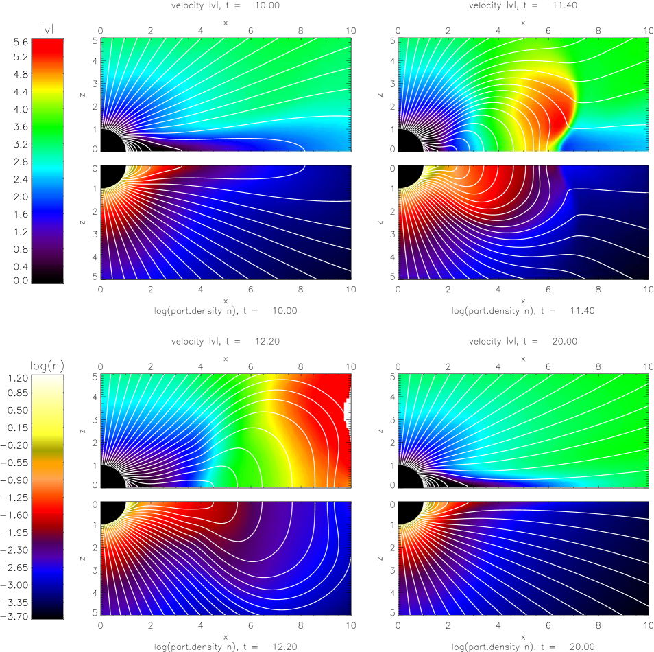
Abbildung 6: Time sequence of simulated CME expansion from pre-eruption ($t=10.0$) to expansion and return to equilibrium (at $t=20.0$), showing contours of $\|\vec{u}\|$ (top) and $\log_{10}n$ (bottom) in the poloidal plane ($y=0$), with magnetic field lines superimposed. The CME speed at onset was chosen to be $u_{\rm cme}=2$. An MPEG movie of this simulation, which covers the entire simulation from initialization ($t=0$) to convergence into steady-state (near $t=10$), CME expansion and back to near-equilibrium ($t\approx 20$), is available from the supplementary material at mpg.

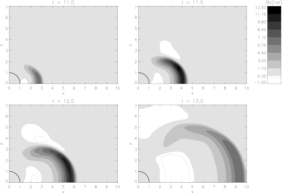
Abbildung 7: Contour plot showing the value of $B_{z}$ in the $(x,y)$ plane, normalized to the corresponding values at the pre-eruptive equilibrium ($t=10.0$). The unit circle marks the position of the solar surface. Note the field reversals occurring within the encircled regions (dotted), most notably in the CME’s wake.

Taking advantage of the fully 3-D nature of our simulations, we can also access the dynamics in the perpendicular planes. Figure 7 shows time frames from the same run, this time viewed as a contour of the sharp, wall-shaped $B_{z}$ signature which arises when the CME runs into the background magnetic field and forces it to pile up ahead of it. As can be expected, the magnetic front moves fastest in the $x$ direction, thus forming an elongated shell around the CME’s core. On the opposite side, the CME’s wake shows a marked reduction in field strength, which even includes an expanding region of reversed field direction trailing the CME. The region’s growing extent is particularly evident from the dotted wedge discernible in Fig. 8. Note that the steep outward slope of $\|\vec{B}\|$ ($\propto r^{-3}$ for a dipole) makes it necessary to normalize the values appropriately.

To analyses the dynamics of the CME as a whole, a reliable tracer of its position is required. While the CME’s density shows relatively large and irregular fluctuations which make it difficult to use it to monitor its location, we found the magnetic field signature of Fig. 7 to be more suitable for this purpose. Figure 8 may serve to illustrate this idea. From the resulting $[t,x(t)]$ curves, we derive terminal velocities of $3.5\ c_{\rm s}\approx 450$ km/s and $4.5\ c_{\rm s}\approx 580$ km/s for CMEs launched with an initial velocity of $u_{\rm cme}=0$ and $2$, respectively.

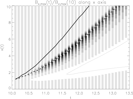
Abbildung 8: Height-time plot tracing the position of the normalized maximum of $B_{z}$, which moves slightly ahead of the actual CME. Each vertical strip can be thought of as a cut along the $x$ axis of Fig. 7 with identical color scale (including the dotted inversion line). The thick dashed line connects the respective maxima, thus forming an $t\mapsto x(t)$ position curve for the magnetic peak leading the CME. The solid line shows the corresponding $x(t)$ plot for the faster CME ($u_{\rm cme}=2$ rather than 0). The corresponding contour stripes for this second CME are not shown.

5.3.2 Interacting CMEs

With the rate of CME occurrence reaching several events per day during solar maximum, it is not unusual to find more than one CME to be present in a given section of interplanetary space, a fact which motivates the numerical study of the interaction of CMEs. Simulations of this kind have been carried out by various authors (Vandas et al., 1997; Odstrčil et al., 2003; Schmidt and Cargill, 2004; Wang et al., 2005). Interacting CMEs have also been linked to the modulation of type II radio bursts (Nunes, 2007), and their importance for SEP generation has been investigated by Gopalswamy et al. (2005) and Vandas and Odstrčil (2004) using 2.5-D flux rope simulations. More recently, Lugaz (2008) has connected earlier simulations (Lugaz et al., 2005, 2007) employing the BATS-R-US code (Manchester et al., 2004) to actual LASCO data by means of synthetic observations. While it is clear that at this initial stage, our simulations cannot be expected to rival the existing work in either detail or scientific content, we can nevertheless demonstrate our code’s general applicability to this important sub-class of CME phenomenae.
Figure 9 shows selected snapshots of a corresponding simulation run: At $t=10$, a slow ($u_{\rm cme,1}=0$) CME is initiated along the $x$ axis, to be quickly followed by a faster one ($u_{\rm cme,2}=2$) launched at $t=11.0$ into the same direction. (Note that this terminology is merely used to distinguish both entities from each other. We do not intend to relate these to the slow/ fast dichotomy known from actual CME observations. As was shown at the end of the preceding section, both simulated CMEs would qualify as ’slow’ in this sense.)
Both CMEs not only exhibit the individual effects of acceleration, expansion, and field line kinking already found and discussed in the previous case of an isolated CME, but there is apparently also a noticeable interaction between the two as the second CME gains speed and eventually collides with its predecessor. Note again the kinked magnetic field lines along with a corresponding density gradient, both related to discontinuities that would develop into shocks in the non-isothermal case. It is also interesting to observe that the prescribed density excess is sufficient to trigger a spontaneous, self-consistent outward acceleration, without the need to artificially ’push’ the CME forward by enforcing a non-zero initial velocity at the instant of its launch.

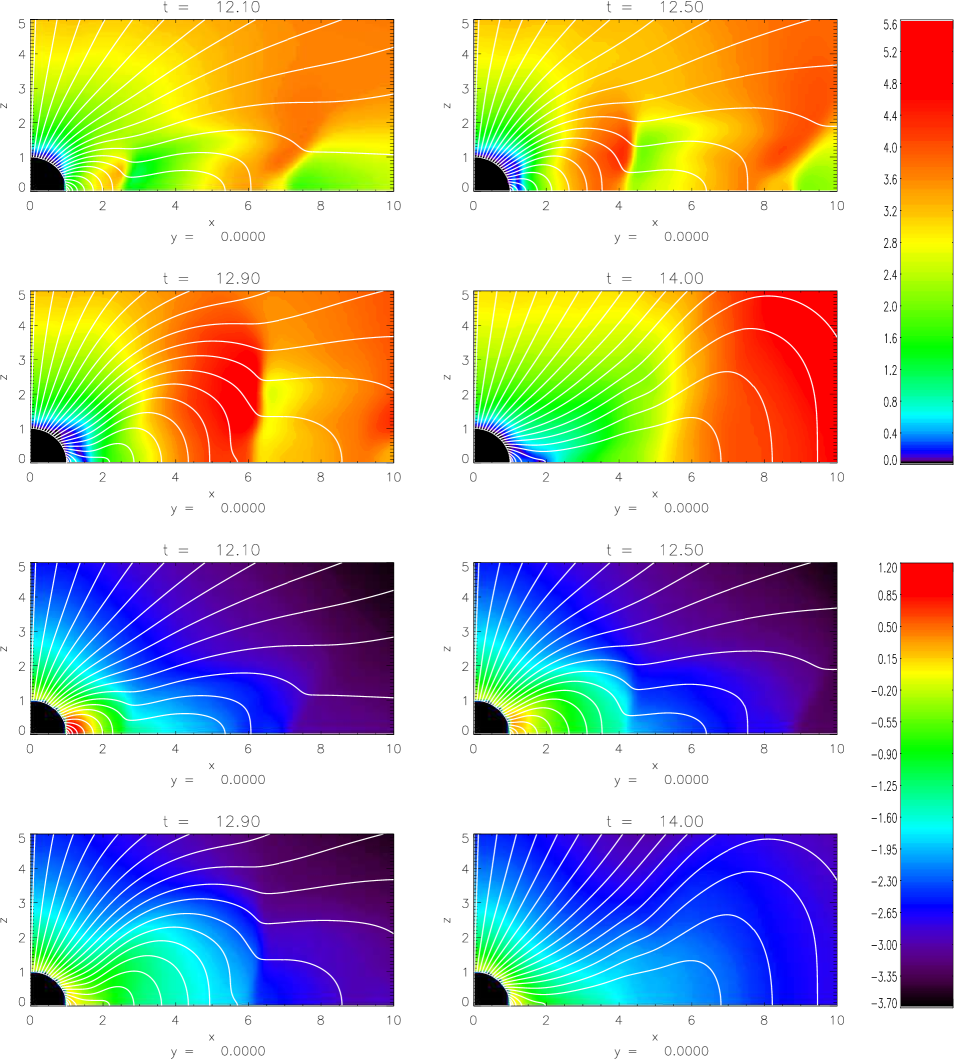
Abbildung 9: Selected snapshots from a simulation of two interacting CMEs showing velocity (top) and decadic logarithm of density (bottom), as well as magnetic field lines (white) in the ($y=0$) plane. The initial and final states are practically identical with the corresponding situation shown in the first and last frame of Fig. 6, and are therefore not repeated here.

5.4 Connecting to observations

Due to lack of in-situ data at small distances from the Sun, a direct comparison between simulation and actual CME data is currently not feasible. In order to at least qualitatively connect the simulations presented here to observations, five fixed locations at radii $r_{b}\in\{2,4,6,8,10\}$ were chosen along the CME’s trajectory (i. e. the $x$ axis). At every time step, the values of the non-vanishing variables $[B_{z},n,u_{x}]$ at these locations were extracted from the simulation data and then combined in the panel of Fig. 10. Thus, a time profile of these quantities is generated, as it would be seen by a stationary observer while the CME moves past his location. (It should be noted that the profiles for particle density $n$ and magnetic field $B_{z}$ at radius $r_{b}$ have been multiplied with $(r_{b})^{3}$ and $-(r_{b})^{2}$, respectively, since otherwise the effect of radial dilution would not have allowed curves of various radii to be presented compactly in a single viewgraph. This obviously only changes the relative size of two profiles against one another but leaves the shapes of individual profiles unchanged.)
Using Fig. 11, these plots can be contrasted with a compilation of the temporal evolution of the solar wind’s MHD properties, as measured by the Advanced Composition Explorer (ACE) for a magnetic cloud passing the probe’s location, the inner Lagrange point at a heliocentric radius of 0.99 AU. A number of qualitative similarities between observation and our simulation can indeed be identified; especially the sharp rise and slow decay of the velocity’s maxima is clearly discernible in both cases. The sharp, almost needle-shaped peaks of the magnetic field profiles also exhibit a striking similarity. These pronounced field enhancements are induced by the CME’s compression wave, and even seem to increase further as the driving CME accelerates outward.
The notable differences in the total duration of passage (about one day for the magnetic cloud opposed to about one hour in the simulations) can easily be accounted for by the very different sites of observation. The cloud had much more time to extend from a presumably rather compact object to its full length of up to 1 AU. Also, the transit time cannot be expected to be totally independent of the duration of CME initiation (which in our case amounts to just 1.5 h real time). However, since observation and simulation stem from very different heliocentric radii, a direct, quantitative comparison between the respective profiles of Figs. 10 and 11 is of course not feasible. Our attempts to identify common features between them can therefore merely serve as a reality checkön the general usefulness of these first simulation runs. Besides, they may serve to illustrate the type of comparison that are intended for future simulations covering the whole radial range up to Earth orbit.

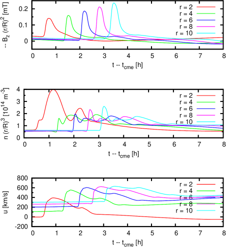
Abbildung 10: Simulated profiles of magnetic field, density, and fluid velocity as seen by static observers situated along the CME expansion direction at radii $r/R_{\odot}\in\{2,4,6,8,10\}$ for the sequence of Fig. 6. The minus sign at $B_{z}$ compensates for the magnetic field’s north-south polarity (which has $B_{z}<0$ at $z=0$). Time is given in hours after CME onset. Temperature profiles are not shown due to $\gamma=1$.

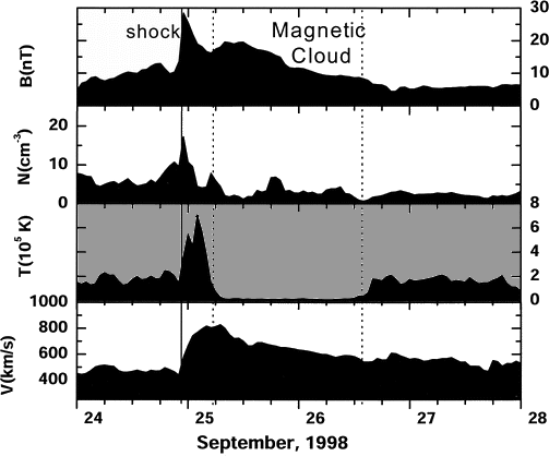
Abbildung 11: Actual in situ measurements of a magnetic cloud near 1 AU, adopted from Burlaga et al. (2001). The general shape of these profiles is to be compared with the simulation results depicted in Fig. 10.

We have reported on the creation of a 3-D MHD model of the near-Sun heliosphere, its numerical implementation and subsequent application to the propagation of CMEs.
In order to adequately implement the Sun’s spherical surface as an inner boundary on the Cartesian grid, a weighted averaging procedure was devised which is able to handle the huge gradients (most notably of mass density) present at this boundary. The use of this procedure also contributed to a reduction of spurious departures from the problem’s underlying symmetry, which result from the fact that the Sun’s spherical (boundary) surface cannot be mapped to a Cartesian grid of finite cell spacing. Comparing a Dirichlet boundary condition for the velocity against free inward extrapolation, the latter was found to yield slightly more accurate results, albeit requiring a more complex numerical implementation. To ensure a solenoidal magnetic field, the GLM scheme was found to be inappropriate due to the presence of internal boundaries, and was thus abandoned in favor of a classical projection method.
After the model’s CWENO-based numerical realization had satisfactorily passed various test cases, it was successfully employed to generate stable, self-consistent MHD equilibria of the quiet, magnetized solar wind. These were then themselves used as initial configurations to simulate the expansion of CME-like plasma bubbles. Since the modelling is fully three-dimensional, the CME’s direction of expansion can be chosen independently of the system’s axis of symmetry; in particular, it is possible to study expansion within the ecliptic plane.
The extracted time profiles of density, flow velocity, and magnetic field strength show qualitative similarities to actual in-situ data obtained from satellites at much larger heliospheric distances. The fact that such similarities can be found lends support to the notion that the main physical processes which shape the structure of a CME occur shortly after onset, whereas the ensuing phase of interplanetary propagation is merely characterized by dilution and (almost) self-similar expansion, although a direct simulation covering the entire range up to Earth orbit will be needed to make unambiguous statements about the CME’s IP evolution and its persistent self-similarity (or lack thereof). In a future extension of this work, we intend to merge heated (i. e. non-isothermal) scenarios with magnetized wind models, a step which, however desirable, could not yet be carried out due to remaining numerical difficulties. This direction seems even more promising since both aspects have been proven to yield satisfactory solutions individually.
On the model side, we plan to include additional aspects (such as localized heating and changes in magnetic topology) into the CME’s initialization to trigger its eruption. Since this will require a much higher grid resolution near the solar surface, a recourse to adaptive mesh refinement and/or parallelization becomes mandatory.