On Non-parametric Estimation of the Lévy Kernel of Markov processes

Abstract

We consider a recurrent Markov process which is an Itô semi-martingale. The Lévy kernel describes the law of its jumps. Based on observations $X_{0},X_{\Delta},\dotsc,X_{n\Delta}$, we construct an estimator for the Lévy kernel’s density. We prove its consistency (as $n\Delta\to\infty$ and $\Delta\to 0$) and a central limit theorem. In the positive recurrent case, our estimator is asymptotically normal; in the null recurrent case, it is asymptotically mixed normal. Our estimator’s rate of convergence equals the non-parametric minimax rate of smooth density estimation. The asymptotic bias and variance are analogous to those of the classical Nadaraya–Watson estimator for conditional densities. Asymptotic confidence intervals are provided.

AMS Subject Classification 2010: Primary 62M05; secondary 62G07, 60F05, 60J25
Keywords: Markov process, Itô semi-martingale, Lévy system, Lévy kernel, null recurrence, density estimation, central limit theorem

This is a preprint of a paper which has been accepted for publication in the journal Stochastic Processes and their Applications on April 30, 2013.

1 Introduction

Statistical inference for jumps in continuous-time models has received significant attention in recent years. Due to their well-known tractability properties, a vast amount of literature has been devoted to the class of processes with stationary and independent increments, called Lévy processes. The law of their jumps is characterised by their Lévy measure. Parametric inference for Lévy measures has a long history. For recent developments in non-parametric settings, we refer, for instance, to Comte and Genon-Catalot (2011); to Figueroa-López (2011); to the special issue Gugushvili et al. (2010), which contains a collection of interesting papers; to Neumann and Reiß (2009); and to Ueltzhöfer and Klüppelberg (2011). Ample references to previous literature can be found within the aforementioned.

In this paper, we consider a Harris recurrent Markov process $X$ which is an Itô semi-martingale. Such a process is a solution of some stochastic differential equation

$$\begin{aligned} \mathrm{d}X_{t}=b(X_{t})\mathrm{d}t+\sigma(X_{t})\mathrm{d}W_{t}&+\int\delta(X_{t-},y)\mathbbm{1}_{\{\lVert\delta(X_{t-},y)\rVert>1\}}\mathfrak{p}(\mathrm{d}t,\mathrm{d}y)\\ &+\int\delta(X_{t-},y)\mathbbm{1}_{\{\lVert\delta(X_{t-},y)\rVert\leq 1\}}(\mathfrak{p}-\mathfrak{q})(\mathrm{d}t,\mathrm{d}y),\end{aligned}$$ (1.1)

with coefficients $b$, $\sigma$ and $\delta$; the SDE is driven by some Wiener process $W$ and some Poisson random measure $\mathfrak{p}$ (with intensity measure $\mathfrak{q}(\mathrm{d}t,\mathrm{d}y)=\mathrm{d}t\otimes\lambda(\mathrm{d}y)$); $X_{t-}$ denotes the left-limit. The law of its jumps is more or less described by the kernel $F$ where, for each $x$, the measure $F(x,\cdot)$ coincides with the image of the measure $\lambda$ under the map $y\mapsto\delta(x,y)$ restricted to the set $\{y:\delta(x,y)\neq 0\}$. We call $F$ the (canonical) Lévy kernel of $X$. We assume that the measures $F(x,\mathrm{d}y)$ admit a density $y\mapsto f(x,y)$, and we aim for non-parametric estimation of the function $(x,y)\mapsto f(x,y)$.

On an equidistant time grid, we observe a sample $X_{0}(\omega),X_{\Delta}(\omega),\dotsc,X_{n\Delta}(\omega)$ of the process; the jumps are latent. We study a kernel density estimator for $f(x,y)$. We show its consistency as $n\Delta\to\infty$ and $\Delta\to 0$ under a smoothness hypothesis on the estimated density. In the ergodic case, we obtain asymptotic normality. In the null recurrent case, we impose a condition on the resolvent of the process which goes back to Darling and Kac (1957). Thereunder, we prove asymptotic mixed normality. We also provide a standardised version of our central limit theorem for the construction of asymptotic confidence intervals.

Our results are comparable to those in classical non-parametric density estimation. In particular: Our estimator’s asymptotic bias and variance resemble those of the Nadaraya–Watson estimator in classical conditional density estimation. Just as in the classical context, moreover, the bandwidth choice is crucial for our estimator’s rate of convergence. We conjecture that, for instance, a cross-validation method applies here analogously; see Fan and Yim (2004) and Hall et al. (2004). By an optimal choice, if $\Delta\to 0$ fast enough, the rate is $v({n\Delta})^{\alpha_{1}\alpha_{2}/[d(\alpha_{1}+\alpha_{2})+2\alpha_{1}\alpha_{2}]}$, where $\alpha_{1}>0$ (resp., $\alpha_{2}>0$) stands for the smoothness of $f$ as a function in $x$ (resp., in $y$), and the function $v$ plays the role of an information rate. In the ergodic case, $v(t)=t$; in the null recurrent case with Darling–Kac’s condition imposed, $v(t)=t^{\delta}\ell(t)$ for some $0<\delta\leq 1$ and some slowly varying function $\ell$. We remark that, in the case $\alpha_{1}=\alpha_{2}$, our achieved rate $v({n\Delta})^{\alpha_{1}/(2\alpha_{1}+2d)}$ equals the non-parametric minimax rate of smooth density estimation, related to the smoothness of $f$ as a $2d$-dimensional function and with respect to $v({n\Delta})$.

At the core of our statistical problem, we essentially have to study the case first, where the process is observed continuously in time and, in particular, all jumps are discerned. In this case, we can consider a more general class of quasi-left-continuous, strong Markov processes with càdlàg sample paths than just Itô semi-martingales. For these, the law of their jumps is again described by their Lévy kernel. We present a version of our estimator which utilises that the sojourn time of certain sets and the jumps are observed. Under slightly weaker assumptions, we prove the estimator’s consistency and asymptotic (mixed) normality. As these results are valid for a quite general class of processes, we believe that they are of independent interest, not only as a benchmark for all possible estimators which are based on some discrete observation scheme.

For discrete-time Markov chains, a related result is presented in Karlsen and Tjøstheim (2001). We are aware that our final steps of proof appear to be similar. We emphasise that the main difficulties in our context, however, come in two respects: on the one hand, from establishing an appropriate auxiliary framework where related methods apply; on the other hand, from the discrete observation scheme where our primary objects of interest – the jumps – are latent.

For continuous-time Markov processes, apart from the Lévy process case and as far as known to us, estimation of their Lévy kernel has been confined to the special case of Markov step processes. For these, there is a one-to-one correspondence between the Lévy kernel and the infinitesimal generator. Efficient non-parametric estimation of Markov step process models has been studied by Greenwood and Wefelmeyer (1994). They assume the mean holding times to be bounded, and the transition kernel to be uniformly ergodic. This excludes the null recurrent case. The work on parametric estimation of Markov step processes is more exhaustive. The null recurrent case has been studied, for instance, by Höpfner (1993). There, the process is observed up to a random stopping time such that a deterministic amount of information (or more) has been discerned. Local asymptotic normality is shown in various situations. With a slightly different aim, in contrast, Höpfner et al. (1990) considers Markov step processes observed up to a deterministic time. Accordingly, the observed amount of information is random. Local asymptotic mixed normality (of statistical experiments) is shown under Darling–Kac’s condition. Here, we utilise some of their results and methods. We improve upon the restrictions within the aforementioned literature: First and foremost, we do not restrict ourselves to Markov step processes. Second, we consider processes, null recurrent in the sense of Harris, in a non-parametric setting. Third, we address the influence of observations on a discrete time grid.

We briefly outline our paper. In section 2 we study the estimation of the Lévy kernel based on discrete observations. Split into three subsections, we present the statistical problem with our standing assumptions; we give our estimator along with a bias correction; and state our main results – the estimator’s consistency and the central limit theorem. In section 3, we study the case where continuous-time observations are available. This section is organised analogously to section 2. The corresponding proofs are in section 4. The proofs for our main results of section 2 are in section 5. Each proofs section comes with its own short outline at its beginning. Since we bring together potential theoretic aspects of Markov processes with functional and martingale limit theory, we put some of our technical considerations off to appendix A.

2 Density estimation of the Lévy kernel from high-frequency observations

2.1 Preliminaries and assumptions

On the filtered probability space(s) $(\Omega,\mathscr{F},(\mathscr{F}_{t})_{t\geq 0},(\operatorname{\mathbbm{P}}^{x})_{x\in E})$, let $X=(X_{t})_{t\geq 0}$ be a Markovian Itô semi-martingale with values in Euclidean space $E=(\mathbbm{R}^{d},\mathscr{B}^{d})$, or a subset thereof, such that $\operatorname{\mathbbm{P}}^{x}(X_{0}=x)=1$ for all $x$. For $n\in\mathbbm{N}$ and $\Delta>0$, we observe $X_{0}(\omega)$ and the increments

$$\Delta^{n}_{k}X(\omega)\coloneqq X_{k\Delta}(\omega)-X_{(k-1)\Delta}(\omega)\quad k=1,\dotsc,n.$$ (2.1)

We emphasise that the jumps of the process are latent.

Throughout this paper, we use the following notation: We abbreviate $E^{\ast}\coloneqq E\setminus\{0\}$. We denote the Dirac measure at $x$ by $\epsilon_{x}$. For $\pi$ an (initial) probability on $E$, we denote the expectation w. r. t. the law $\operatorname{\mathbbm{P}}^{\pi}\coloneqq\int\pi(\mathrm{d}x)\operatorname{\mathbbm{P}}^{x}$ by $\operatorname{\mathbbm{E}}^{\pi}$. For $\alpha\geq 0$ and $A\subseteq E$, in addition, $\mathcal{C}^{\alpha}_{\mathrm{loc}}(A)$ denotes the class of all continuous functions on $A$ which are $\lfloor\alpha\rfloor$-times continuously differentiable such that every $x\in A$ has a neighbourhood on which the function’s (partial) $\lfloor\alpha\rfloor$-derivatives are uniformly Hölder of order $\alpha-\lfloor\alpha\rfloor$.

The characteristics $(B,C,\mathfrak{n})$ of $X$ are absolutely continuous with respect to Lebesgue measure; there are mappings $b:E\to E$ and $c:E\to E\otimes E$ (with $c=\sigma\sigma{}^{{}^{\intercal}}$ in view of eq. 1.1), and a kernel $F$ on $E$ with $F(x,\{0\})=0$ such that

$$B_{t}=\int_{0}^{t}b(X_{s})\mathrm{d}s,\quad C_{t}=\int_{0}^{t}c(X_{s})\mathrm{d}s,\quad\text{and}\quad\mathfrak{n}(\mathrm{d}t,\mathrm{d}y)=\mathrm{d}t\otimes F(X_{t},\mathrm{d}y).$$ (2.2)

The integer-valued random measure $\sum_{\{s:\Delta X_{s}\neq 0\}}\epsilon_{(s,\Delta X_{s})}(\mathrm{d}t,\mathrm{d}y)$ on $\mathbbm{R}_{+}\times\mathbbm{R}^{d}$ is called the process’s jump measure. The random measure $\mathfrak{n}$ is its predictable compensator: For every Borel function $g:E\times E\to\mathbbm{R}_{+}$, (inital) probability $\pi$, and $t>0$, we have

$$\operatorname{\mathbbm{E}}^{\pi}\sum_{0<s\leq t}g(X_{s-},\Delta X_{s})\mathbbm{1}_{\{X_{s-}\neq X_{s}\}}=\operatorname{\mathbbm{E}}^{\pi}\int_{0}^{t}\mathrm{d}s\int_{E}F(X_{s},\mathrm{d}y)g(X_{s},y).$$ (2.3)

We call $F$ the Lévy kernel. It is unique outside a set of potential zero. We assume it admits a density $(x,y)\mapsto f(x,y)$ which we want to estimate.

Throughout, we work under the following technical hypothesis on the characteristics:

2.1 Assumption.

1. The process $X$ satisfies the following (linear) growth condition: There exists a constant $\zeta<\infty$ and a Lévy measure $\bar{F}$ on $E$ such that

   $$\lVert b(x)\rVert\leq\zeta(1+\lVert x\rVert),\quad\lVert c(x)\rVert\leq\zeta(1+\lVert x\rVert^{2}),\quad\text{and}\quad F(x,A)\leq(1+\lVert x\rVert)\bar{F}(A)$$

   holds for all $x\in E$ and every Borel set $A\subseteq E$. We denote by $\beta\in[0,2]$ some constant such that $\int\bar{F}(\mathrm{d}w)(\lVert w\rVert^{\beta}\wedge 1))<\infty$.

2. The Lévy measure $\bar{F}$ admits a density $\bar{f}$ which is continuous on $E^{\ast}$.

3. There exists a constant $\zeta<\infty$ such that $\sup_{\lVert z\rVert>1}\lVert z\rVert\bar{f}(z)\leq\zeta$.

_⋄

Remark.

Apart from the growth condition, there is no assumption on $b$ and $c$. Whether $X$ is a weak or a strong solution of eq. 1.1 is irrelevant to us.

We impose assumptions on the recurrence of $X$ and on the smoothness of $f$. To obtain consistency for our estimator below, we impose:

2.2 Assumption.

The process $X$ is Harris recurrent: On $E$, there exists a $\sigma$-finite, invariant measure $\mu$ for $X$ such that, for every Borel set $A\subseteq E$, we have

$$\mu(A)>0\implies\operatorname{\mathbbm{P}}^{x}\left(\int\nolimits_{0}^{\infty}\mathbbm{1}_{A}(X_{s})\mathrm{d}s=\infty\right)=1\quad\forall x\in E.$$

_⋄

2.3 Assumption.

For some $\alpha>0$, the Lévy kernel admits a density $f\in\mathcal{C}^{\alpha}_{\mathrm{loc}}(E\times E^{\ast})$; and the invariant measure from Assumption 2.2 admits a continuous density $\mu^{\prime}$. _⋄

Remark.

Harris recurrence can be verified, for instance, by virtue of a Foster–Lyapunov type criteria (see Meyn and Tweedie, 1993b). Moreover, for the existence of a smooth density $\mu^{\prime}$ it is sufficient that the marginal distributions of $X_{t}$ admit a smooth density. We refer, for instance, to Picard (1996) for criteria for the latter.

To obtain a central limit theorem, we also impose:

2.4 Assumption.

The process $X$ satisfies the following Darling–Kac condition: For some $0<\delta\leq 1$, there exists a function $v:\mathbbm{R}_{+}\to\mathbbm{R}_{+}$ – at infinity, regularly varying of index $\delta$ – such that, for every $\mu$-integrable $g$,

$$\frac{1}{v(1/\lambda)}\int_{0}^{\infty}\mathrm{e}^{-\lambda t}\operatorname{\mathbbm{E}}^{x}[g(X_{t})]\mathrm{d}t\to\mu(g)\quad\mu\text{-a.\,e. as }\lambda\downarrow 0.$$ (2.4)

_⋄

Remark.

In the positive recurrent case (that is, when $\mu$ is finite), Assumption 2.4 indeed is satisfied for $\delta=1$ and with $v(t)=t/\mu(E)$. We refer the interested reader to Touati (1987) and to Höpfner and Löcherbach (2003).

2.5 Assumption.

For some $\alpha_{1},\alpha_{2}\geq 2$, the Lévy kernel admits a density $f$ which is twice continuously differentiable on $E\times E^{\ast}$ such that $x\mapsto f(x,y)\in\mathcal{C}^{\alpha_{1}}_{\mathrm{loc}}(E)$ for all $y\in E^{\ast}$, and $y\mapsto f(x,y)\in\mathcal{C}^{\alpha_{2}}_{\mathrm{loc}}(E^{\ast})$ for all $x\in E$; and the invariant measure from Assumption 2.2 admits a continuous density $\mu^{\prime}$ which is $(\lceil\alpha_{1}\rceil-1)$-times continuously differentiable. _⋄

Example.

Suppose that $f$ is bounded and vanishes outside $\{\lVert x\rVert\leq 1,\lVert y\rVert\leq 1\}$; that is, there are neither jumps with left-limit outside the unit ball nor jumps of size bigger than one. Then our process’s recurrence (or transience) is completely determined by drift and volatility. For instance:

1. If the volatility $\sigma$ vanishes everywhere and the drift satisfies $b(x)=-x$, then $X$ is positive recurrent.

2. If the drift $b$ vanishes everywhere, and the volatility satisfies $\sigma(x)=1$, then $X$ is not positive. In fact, $X$ has the recurrence (or transience) of Brownian motion: In the univariate case, $X$ is null recurrent and Darling–Kac’s condition holds with $\delta=1/2$; in the bivariate case, $X$ is null recurrent and Darling–Kac’s condition fails; and in all other multivariate cases, $X$ is transient.

2.2 Kernel density estimator

In principle, we are free to choose our favourite estimation method, e. g., the method of sieves with projection estimators. Here, however, we introduce a kernel density estimator as it allows for a more comprehensible presentation of the proofs. Also, the method is well-understood in the context of classical (conditional) density estimation.

An outline: First, we choose smooth kernels $g_{1}$ and $g_{2}$ with support $B_{1}(0)$ (the unit ball centred at zero) which are, at least, of order $\alpha_{1}$ and $\alpha_{2}$, respectively; that is, for every multi-index $m=(m_{1},\dotsc,m_{d})\in\mathbbm{N}^{d}\setminus\{0\}$ and each $i\in\{1,2\}$, we have

$$|m|\coloneqq m_{1}+\dotsb+m_{d}<\alpha_{i}\implies\kappa_{m}(g_{i})\coloneqq\int x_{1}^{m_{1}}\cdot\dotsb\cdot x_{d}^{m_{d}}g_{i}(x)\mathrm{d}x=0.$$ (2.5)

Second, we choose a bandwidth vector $\eta=(\eta_{1},\eta_{2})>0$. Last, we construct an estimator for $f(x,y)$ using the kernels $g_{i}^{\eta,x}(z)\coloneqq\eta_{i}^{-d}g_{i}((z-x)/\eta_{i})$. If the bandwidth is chosen appropriately, we achieve a consistent estimator which follows a central limit theorem.

2.6 Definition.

For $\eta=(\eta_{1},\eta_{2})>0$, we call $\hat{f}^{\Delta,\eta}_{n}$ defined by

$$\hat{f}^{\Delta,\eta}_{n}(x,y)\coloneqq\begin{cases}\frac{\sum_{k=1}^{n}g_{1}^{\eta,x}(X_{(k-1)\Delta})g_{2}^{\eta,y}(\Delta^{n}_{k}X)}{\Delta\sum_{k=1}^{n}g_{1}^{\eta,x}(X_{(k-1)\Delta})}&\text{if }\sum_{k=1}^{n}g_{1}^{\eta,x}(X_{(k-1)\Delta})>0,\\ 0&\text{otherwise},\end{cases}$$ (2.6)

the kernel density estimator of $f$ (w. r. t. bandwidth $\eta$ based on $X_{0},X_{\Delta},\dotsc,X_{n\Delta}$). _⋄

In analogy to classical conditional density estimation, we also introduce a bias correction for our estimator.

2.7 Definition.

For $\eta=(\eta_{1},\eta_{2})>0$, we call $\hat{\gamma}^{\Delta,\eta}_{n}$ defined by

$$\hat{\gamma}^{\Delta,\eta}_{n}(x,y)\coloneqq{}\begin{cases}\begin{aligned} \lx@intercol\@ADDCLASS{ltx_eqn_lefteqn}$\displaystyle\eta_{1}^{\alpha_{1}}\sum_{\begin{subarray}{c}|m_{1}+m_{2}|=\alpha_{1}\\ |m_{2}|\neq 0\end{subarray}}\frac{\kappa_{m_{1}+m_{2}}(g_{1})}{m_{1}!m_{2}!}\frac{\sum_{k=1}^{n}\frac{\partial^{m_{1}}}{\partial x^{m_{1}}}g_{1}^{\eta,x}(X_{(k-1)\Delta})}{\sum_{k=1}^{n}g_{1}^{\eta,x}(X_{(k-1)\Delta})}\frac{\partial^{m_{2}}}{\partial x^{m_{2}}}\hat{f}^{\Delta,\eta}_{n}(x,y)$\mbox{}\hfil\lx@intercol\\ &\hskip 5.0pt+\eta_{2}^{\alpha_{2}}\sum_{|m|=\alpha_{2}}\frac{\kappa_{m}(g_{2})}{m!}\frac{\partial^{m}}{\partial y^{m}}\hat{f}^{\Delta,\eta}_{n}(x,y),&&\text{if }\genfrac{}{}{0.0pt}{}{\sum_{k=1}^{n}g_{1}^{\eta,x}(X_{(k-1)\Delta})>0}{\alpha_{1},\alpha_{2}\in\mathbbm{N}^{\ast}},\\ &0,&&\text{otherwise},\end{aligned}\end{cases}$$

the bias correction for $\hat{f}^{\Delta,\eta}_{n}$. (The sums in the previous equation are over all multi-indices of appropriate length.) _⋄

2.3 Consistency and central limit theorem

Here, we present our main results. We agree to the following conventions: Under Assumptions 2.2 and 2.4, $v$ denotes the regularly varying function given in eq. 2.4. Under Assumption 2.2 only, $v$ denotes an arbitrary deterministic equivalent (see Definition 4.1 below) of the Markov process $X$. For typographical reasons, we may write $v_{t}$ for $v(t)$ or $X(t)$ for $X_{t}$ etc. as convenient.

We utilise the following conditions as $n\Delta\to\infty$ and $\Delta\to 0$, where $0\leq\zeta_{1},\zeta_{2}<\infty$:

$$v_{n\Delta}\eta_{1,n}^{d}\eta_{2,n}^{d}\to\infty, \quad\text{and}\quad\eta_{1,n}\to 0,\quad\eta_{2,n}\to 0;$$ (2.7)

$$v_{n\Delta}\eta_{1,n}^{d+2\alpha_{1}}\eta_{2,n}^{d}\to\zeta_{1}^{2}, \quad\text{and}\quad v_{n\Delta}\eta_{1,n}^{d}\eta_{2,n}^{d+2\alpha_{2}}\to\zeta_{2}^{2};$$ (2.8)

In addition, we also utilise the following conditions due to discretisation, where $\zeta<\infty$ is independent of $n$:

$$\Delta\eta_{1,n}^{-2-d[(1-2/(\beta+d))\vee 0]}\to 0, \quad\text{and}\quad\Delta\eta_{2,n}^{-2\vee(\beta+d)}\to 0;$$ (2.9a)

$$n\Delta^{2}\eta_{1,n}^{d}\eta_{2,n}^{d}\leq\zeta, \quad v_{n\Delta}\Delta^{2}\eta_{1,n}^{d-4-2d[(1-2/(\beta+d)\wedge 0]}\eta_{2,n}^{d}\to 0,$$ (2.9b)

$$\quad\text{and}\quad v_{n\Delta}\Delta^{2}\eta_{1,n}^{d}\eta_{2,n}^{d-4\vee 2(\beta+d)}\to 0.$$ (2.9c)

Remark.

If $\Delta\to 0$ fast enough, then eq. 2.7 and eq. 2.8 are the crucial conditions.

2.8 Theorem.

Grant Assumptions 2.1, 2.3 and 2.2. Let $\eta_{n}=(\eta_{1,n},\eta_{2,n})$ be such that eq. 2.7 and eq. 2.9a hold. Moreover, let $(x,y)\in E\times E^{\ast}$ be such that $\mu^{\prime}(x)>0$ and $F(x,E)>0$.

1. If $n\Delta^{2}\to 0$, then, under any law $\operatorname{\mathbbm{P}}^{\pi}$, we have the following convergence in probability:

   $$\hat{f}_{n}^{\Delta,\eta_{n}}(x,y)\xrightarrow[{n\to\infty}]{\operatorname{\mathbbm{P}}^{\pi}}f(x,y).$$ (2.10)

2. Grant Assumption 2.4 in addition. If $(n\Delta)^{1-\delta}\Delta\to 0$, then, under any law $\operatorname{\mathbbm{P}}^{\pi}$, eq. 2.10 holds as well.

Remark.

By this theorem, our estimator is consistent for every $x$ and $y\neq 0$ if $n\Delta\to\infty$ and $\Delta\to 0$. In practice, however, both $n$ and $\Delta$ are given! Then, for instance, if a continuous martingale component is present, or if there are infinitely many jumps over finite time intervals, our estimator is unreliable for all $y$ close to the origin. To illustrate this important point, suppose that $X$ is a univariate process with constant volatility $\sigma^{2}>0$. Increments with absolute value less than $\zeta\sigma\Delta^{1/2}$, where $\zeta$ is quite a large constant (e. g., $\zeta=5$), are predominantly due to the continuous martingale and not due to jumps. On the set $\{y:|y|\leq\zeta\sigma\Delta^{1/2}\}$, therefore, our estimator $\hat{f}^{\Delta,\eta}_{n}(x,\cdot)$ is unreliable regardless of the chosen bandwidth $\eta$.

For the next theorem, we establish additional notation. For $0<\alpha<1$, let $K$ denote the $\alpha$-stable Lévy subordinator with Laplace transform $\operatorname{\mathbbm{E}}\mathrm{e}^{-\xi K_{t}}=\mathrm{e}^{-t\xi^{\alpha}}$ for $\xi,t\geq 0$. Its right inverse $L_{t}\coloneqq\inf\{s>0:K_{s}>t\}$ is called the Mittag-Leffler process of order $\alpha$. By abuse of notation, we call $L_{t}=t$ the Mittag-Leffler process of order $1$. On an extension

$$(\tilde{\Omega},\tilde{\mathscr{F}},\tilde{\operatorname{\mathbbm{P}}})\coloneqq(\Omega\times\Omega^{\prime},\mathscr{F}\otimes\mathscr{F}^{\prime},\operatorname{\mathbbm{P}}^{\pi}\otimes\operatorname{\mathbbm{P}}^{\prime})$$ (2.11)

of the probability space, let $V=(V(x,y))_{x\in E,y\in E^{\ast}}$ be a standard Gaussian white noise random field (that is, the finite dimensional marginals of $V$ are i. i. d. standard normal) and let $L=(L_{t})_{t\geq 0}$ be the Mittag-Leffler process of order $\delta$ (from Assumption 2.4) such that $V$, $L$ and $\mathscr{F}$ are independent. In the theorem below, convergence holds stably in law; that is, pre-limiting and limiting random variables are defined on the extended space eq. 2.11 and we have joint convergence in law of our pre-limiting random variables with any bounded, $\mathscr{F}$-measurable random variable. This notion, labelled $\mathscr{L}\mathrm{-st}$, is due to Renyi (1963).

2.9 Theorem.

Grant Assumptions 2.1, 2.3, 2.2, 2.4 and 2.5. Let $\eta_{n}=(\eta_{1,n},\eta_{2,n})$ be such that eq. 2.7 and eq. 2.9 hold, and let $(x_{i},y_{i})_{i\in I}$ be a finite family of pairwise distinct points in $E\times E^{\ast}$ such that $\mu^{\prime}(x_{i})>0$ and $F(x_{i},E)>0$ for each $i\in I$. If $(n\Delta)^{1-\delta}\Delta\to 0$, then, under any law $\operatorname{\mathbbm{P}}^{\pi}$, we have the following stable convergence in law:

$$\left(\sqrt{v_{n\Delta}\eta_{1,n}^{d}\eta_{2,n}^{d}}\big{(}\hat{f}_{n}^{\Delta,\eta_{n}}(x_{i},y_{i})-\frac{\mu(g_{1}^{\eta_{n},x_{i}}Fg_{2}^{\eta_{n},y_{i}})}{\mu(g_{1}^{\eta_{n},x_{i}})}\big{)}\right)_{i\in I}\xrightarrow[{n\to\infty}]{\mathscr{L}\mathrm{-st}}\left(\frac{\sigma(x_{i},y_{i})}{\sqrt{L_{1}}}V(x_{i},y_{i})\right)_{i\in I},$$

where the asymptotic variance is given by

$$\sigma(x,y)^{2}\coloneqq\frac{f(x,y)}{\mu^{\prime}(x)}\int g_{1}(w)^{2}\mathrm{d}w\int g_{2}(z)^{2}\mathrm{d}z.$$ (2.12)

In addition, let $\eta_{n}$ be such that eq. 2.8 holds as well. Suppose either that $\alpha_{1},\alpha_{2}\in\mathbbm{N}^{\ast}$ or that $\zeta_{1}=\zeta_{2}=0$ in eq. 2.8. Then, under any law $\operatorname{\mathbbm{P}}^{\pi}$, we have the following stable convergence in law:

$$\left(\sqrt{v_{n\Delta}\eta_{1,n}^{d}\eta_{2,n}^{d}}\big{(}\hat{f}^{\Delta,\eta_{n}}_{n}(x_{i},y_{i})-f(x_{i},y_{i})\big{)}\right)_{i\in I}\xrightarrow[{t\to\infty}]{\mathscr{L}\mathrm{-st}}\left(\gamma(x_{i},y_{i})+\frac{\sigma(x_{i},y_{i})}{\sqrt{L_{1}}}V(x_{i},y_{i})\right)_{i\in I},$$

where – in the former case – the asymptotic bias $\gamma(x,y)$ is given by

$$\begin{aligned} \gamma(x,y)={}&\frac{\zeta_{1}}{\mu^{\prime}(x)}\sum_{\begin{subarray}{c}|m_{1}+m_{2}|=\alpha_{1}\\ |m_{2}|\neq 0\end{subarray}}\frac{\kappa_{m_{1}+m_{2}}(g_{1})}{m_{1}!m_{2}!}\frac{\partial^{m_{1}}}{\partial x^{m_{1}}}\mu^{\prime}(x)\frac{\partial^{m_{2}}}{\partial x^{m_{2}}}f(x,y)\\ &\hskip 150.00023pt+\zeta_{2}\sum_{|m|=\alpha_{2}}\frac{\kappa_{m}(g_{2})}{m!}\frac{\partial^{m}}{\partial y^{m}}f(x,y),\end{aligned}$$ (2.13)

and – in the latter case – $\gamma(x,y)=0$.

Remark.

The asymptotic bias and variance of our estimator are analogous to those of the Nadaraya–Watson estimator in classical conditional density estimation: $\kappa_{m}(g_{i})$ and $\int g_{i}(z)^{2}\mathrm{d}z$ are the relevant moment and the roughness of the kernel $g_{i}$, respectively; and $f$ (resp., $\mu^{\prime}$) plays the role of the conditional (resp., marginal) density.

We recall that $v$ from eq. 2.4 satisfies $v_{t}=t$ in the ergodic case, and $v_{t}=t^{\delta}\ell(t)$ for some slowly varying function $\ell$ in the null recurrent case. If we choose $\eta_{i,n}=v_{n\Delta}^{-\xi_{i}}$ with $\xi_{1}=\alpha_{2}/[d(\alpha_{1}+\alpha_{2})+2\alpha_{1}\alpha_{2}]$ and $\xi_{2}=\alpha_{1}/[d(\alpha_{1}+\alpha_{2})+2\alpha_{1}\alpha_{2}]$, then eq. 2.7 and eq. 2.8 hold with $\zeta_{1}=\zeta_{2}=1$. If $\Delta\to 0$ fast enough such that $n\Delta^{1+[d(\alpha_{1}+\alpha_{2})+2\alpha_{1}\alpha_{2}]/\zeta}\to 0$ in addition, where $\zeta$ denotes the maximum of $(1-\delta)d(\alpha_{1}+\alpha_{2})+2\alpha_{1}\alpha_{2}$, $\delta\alpha_{1}(\alpha_{2}+2+d)$ and $\delta\alpha_{2}(\alpha_{1}+2+d^{2}/(2+d))$, then our choice of $\eta_{n}$ also satisfies eq. 2.9 for every $\beta\leq 2$. Consequently, our estimator’s rate of convergence is

$$v_{n\Delta}^{\alpha_{1}\alpha_{2}/[d(\alpha_{1}+\alpha_{2})+2\alpha_{1}\alpha_{2}]}.$$ (2.14)

In the case $\alpha_{1}=\alpha_{2}{\eqqcolon\alpha}$, the achieved rate $v_{n\Delta}^{\alpha/(2\alpha+2d)}$ equals the non-parametric minimax rate of smooth density estimation, related to the smoothness of $f$ as a $2d$-dimensional function and w. r. t. $v_{n\Delta}$.

Remark.

Bandwidth selection has always been a crucial issue in these kind of studies. Although orders of magnitude are crucial from an asymptotic point of view and $\eta_{i,n}=(n\Delta)^{-\xi_{i}}$ for some $\xi_{i}>0$ may be a good choice , we note that, in practice, $\eta_{i,n}=\zeta(n\Delta)^{-\xi_{i}}$ with leading constant $\zeta\neq 1$ could be a better one. A detailed analysis would go beyond the scope of this paper. We briefly comment on two problems: How to choose the bandwidths manually such that conditions (2.7–2.9) are satisfied for the unknown $v_{n\Delta}$, $\alpha_{1}$, $\alpha_{2}$ and $\beta$? What needs to be considered when employing data-driven methods for selecting optimal bandwidths?

1. Let $\alpha_{0}\geq 2$ and $0<\delta_{0}\leq 1$ such that $\delta_{0}>d/(d+\alpha_{0})$. If we choose $\eta_{i,n}=(n\Delta)^{-1/(2d+2\alpha_{0})}$, then eq. 2.7 and eq. 2.8 hold for all processes $X$ such that Assumptions 2.5 and 2.4 hold for some $\alpha_{1},\alpha_{2}\geq\alpha_{0}$ and $\delta_{0}<\delta\leq 1$. If $\Delta\to 0$ fast enough such that $n\Delta^{1+2[\alpha_{0}+d]/[\alpha_{0}+(2+d)\vee\alpha_{0}]}\to 0$ in addition, then our chosen bandwidth also satisfies eq. 2.9.

2. The asymptotic bias and variance are proportional to the value of $f$ and its derivatives at the point of interest. The optimal bandwidth choice in terms of the asymptotic mean squared error, therefore, may depend heavily on $x$ and $y$. Especially for processes with infinite activity – where $y\mapsto f(x,y)$ has a pole at zero – this is an important issue in practice; cf.  simulations in appendix B. In a future study on data-driven bandwidth selection methods like cross-validation, this distinction from estimating a bounded probability density has to be addressed carefully.

Theorem 2.9 does not allow for a direct construction of confidence intervals. For this purpose, we also obtain the following standardised version.

2.10 Corollary.

Grant Assumptions 2.1, 2.2, 2.3, 2.4 and 2.5. Let $\eta_{n}=(\eta_{1,n},\eta_{2,n})$ be such that (2.7–2.9) hold. Suppose either that $\alpha_{1},\alpha_{2}\in\mathbbm{N}^{\ast}$ or that $\zeta_{1}=\zeta_{2}=0$ in eq. 2.8. Then under any law $\operatorname{\mathbbm{P}}^{\pi}$, we have the following stable convergence in law:

$$\left(\sqrt{\frac{\eta_{1,n}^{d}\eta_{2,n}^{d}\Delta\sum_{k=1}^{n}g_{1}^{\eta_{n},x_{i}}(X_{(k-1)\Delta})}{\xi_{g}^{2}\hat{f}_{n}^{\Delta,\eta_{n}}(x_{i},y_{i})}}\big{(}[\hat{f}_{n}^{\Delta,\eta_{n}}-\hat{\gamma}^{\eta_{n}}_{n}-f](x_{i},y_{i})\big{)}\right)_{i\in I}\xrightarrow[{n\to\infty}]{\mathscr{L}\mathrm{-st}}\big{(}V(x_{i},y_{i})\big{)}_{i\in I},$$

where $\xi_{g}^{2}=\int g_{1}(w)^{2}\mathrm{d}w\int g_{2}(z)^{2}\mathrm{d}z$.

Remark.

In principle, the results of this section are extendible to more general Markov models with Lévy kernel $F$ such that eq. 2.3 holds. In view of our proofs, the assumption that $X$ is an Itô semi-martingale is crucial for the analysis of the influence of discretisation (see section 5.1). Suppose that an explicit upper bound for the small-time asymptotic “error”

$$\left|\frac{1}{\Delta}\operatorname{\mathbbm{E}}^{x}\left[g_{2}^{\eta,y}(\Delta_{1}^{n}X)\right]-\int F(x,\mathrm{d}w)g_{2}^{\eta,y}(w)\right|$$

and an explicit sufficient condition which ensures

$$\sup_{s\leq 1}\frac{\xi_{n}}{v_{n\Delta}\eta_{1,n}^{d}}\left|{\Delta}\sum_{k=1}^{\lfloor sn\rfloor}h_{n}(X_{(k-1)\Delta})-\int_{0}^{\lfloor sn\rfloor\Delta}h_{n}(X_{r})\mathrm{d}r\right|\xrightarrow[{n\to\infty}]{\operatorname{\mathbbm{P}}^{\pi}}0$$

for $\xi_{n}=1$ or $\xi_{n}^{2}=v_{n\Delta}\eta_{1,n}^{d}\eta_{2,n}^{d}$ are available for some Markov process $X$. Then it is straightforward (see Lemmata 5.7 and 5.32 — Lemmata 5.6, 5.9 and 5.10, respectively) to come up with sufficient conditions for Theorems 2.8 and 2.9, which replace eq. 2.9.

3 Density estimation of the Lévy kernel from continuous-time observations — A benchmark

The Lévy kernel of a Markov process is related with jumps. In fact, our estimator eq. 2.6 uses $X_{(k-1)\Delta}$ and $\Delta^{n}_{k}X$ as proxies for the pre-jump value $X_{t-}$ and the jump size $\Delta X_{t}$ if, at a time $t\in[(k-1)\Delta,k\Delta]$, there is a jump from a neighbourhood of $x$ and of size close to $y$. Eventually, such time intervals contain either zero or one such jump; never more. Certainly, the statistical analysis simplifies if we observed the whole path of $X$; introducing proxies would be useless. So, despite observing the whole path of $X$ is somewhat unrealistic, it is theoretically important to study what happens in this case. This section is devoted to this question and can be viewed as a benchmark for what properties are achievable with a more realistic, discrete observation scheme.

3.1 Preliminaries and assumptions

On the filtered probability space(s) $(\Omega,\mathscr{F},(\mathscr{F}_{t})_{t\geq 0},(\operatorname{\mathbbm{P}}^{x})_{x\in E})$, let $X=(X_{t})_{t\geq 0}$ be a strong Markov process with values in Euclidean space $E=(\mathbbm{R}^{d},\mathscr{B}^{d})$, or a subset thereof. Its sample paths are supposed to be càdlàg. We observe – continuously in time – one sample path $\{X_{s}(\omega):s\in[0,t]\}$ for $t>0$; in particular, we discern all jumps.

In addition to the notation introduced before, we use some classical notation from Getoor (1975): We denote the shift semi-group on $\Omega$ by $(\theta_{t})_{t\geq 0}$ so that $X_{t+s}=X_{t}\circ\theta_{s}$ for all $s,t\geq 0$. We denote the transition semi-group of $X$ on $E$ by $(P_{t})_{t\geq 0}$.

A (perfect homogeneous) additive functional $H$ of $X$ is an $\mathscr{F}_{t}$-adapted process such that $H_{t+s}=H_{t}\circ\theta_{s}+H_{s}$ for all $s,t\geq 0$. A Lévy system $(F,H)$ of $X$ (in a wide sense) is a kernel $F$ on $E$ with $F(x,\{0\})=0$ and a non-decreasing additive functional $H$ of $X$ such that, for every Borel function $g:E\times E\to\mathbbm{R}_{+}$, probability $\pi$ on $E$, and $t>0$,

$$\operatorname{\mathbbm{E}}^{\pi}\sum_{0<s\leq t}g(X_{s-},\Delta X_{s})\mathbbm{1}_{\{X_{s-}\neq X_{s}\}}=\operatorname{\mathbbm{E}}^{\pi}\int_{0}^{t}\mathrm{d}H_{s}\int_{E}F(X_{s},\mathrm{d}y)g(X_{s},y).$$ (3.1)

The disintegration into $F$ and $H$ is by no means unique. For an appropriate reference function $g_{0}$ with $Fg_{0}(x)>0$, nevertheless, ratios of the form $Fg(x)/Fg_{0}(x)$ are unique outside a set of potential zero. In the cases where $X$ is quasi-left-continuous (that is, when all jump times are totally inaccessible) Benveniste and Jacod (1973) proved the existence of a Lévy system $(F,H)$ where $H$ is continuous. Such a process – càdlàg, strong Markov, quasi-left-continuous – is called a Hunt process.

Remark.

The continuity of the additive functional was included as a part of the original definition of Lévy systems due to Watanabe (1964).

Throughout this section, we work under the following hypothesis:

3.1 Assumption.

There exists a Lévy system $(F,H)$ of $X$ where $H_{t}=t$. _⋄

Recalling eq. 2.3, we observe that all Markovian Itô semi-martingales satisfy Assumption 3.1. In analogy to the semi-martingale case, we call this $F$ in Assumption 3.1 the (canonical) Lévy kernel of $X$. It is unique outside a set of potential zero. Again, we assume it admits a density $(x,y)\mapsto f(x,y)$ which we want to estimate.

Compared to section 2, we slightly weaken the assumptions imposed on the smoothness of $f$. To obtain consistency for our estimator below, we impose Assumption 2.2 and:

3.2 Assumption.

The canonical Lévy kernel admits a density $f$, continuous on $E\times E^{\ast}$; and the invariant measure from Assumption 2.2 admits a continuous density $\mu^{\prime}$. _⋄

To obtain a central limit theorem, we also impose Assumption 2.4 and:

3.3 Assumption.

For some $\alpha_{1},\alpha_{2}>0$, the canonical Lévy kernel admits a density $f$ such that $x\mapsto f(x,y)\in\mathcal{C}^{\alpha_{1}}_{\mathrm{loc}}(E)$ for all $y\in E^{\ast}$, and $y\mapsto f(x,y)\in\mathcal{C}^{\alpha_{2}}_{\mathrm{loc}}(E^{\ast})$ for all $x\in E$; and the invariant measure from Assumption 2.2 admits a continuous density $\mu^{\prime}$ which is $(\lceil\alpha_{1}\rceil-1)$-times continuously differentiable. _⋄

3.2 Kernel density estimator

In section 2.2, we introduced a kernel density estimator and its bias correction based on discrete observations. Here, we present corresponding versions which utilise the continuous-time observation scheme. We recall that $g_{1}$ and $g_{2}$ are kernels with support $B_{1}(0)$ which are, at least, of order $\alpha_{1}$ and $\alpha_{2}$, respectively. Given some bandwidth vector $\eta=(\eta_{1},\eta_{2})>0$, we utilise the kernels $g_{i}^{\eta,x}(z)=\eta_{i}^{-d}g_{i}((z-x)/\eta_{i})$.

3.4 Definition.

For $\eta=(\eta_{1},\eta_{2})>0$, we call $\hat{f}^{\eta}_{t}$ defined by

$$\hat{f}^{\eta}_{t}(x,y)\coloneqq\begin{cases}\frac{\sum_{0<s\leq t}g_{1}^{\eta,x}(X_{s-})g_{2}^{\eta,y}(\Delta X_{s})\mathbbm{1}_{\{X_{s-}\neq X_{s}\}}}{\int_{0}^{t}g_{1}^{\eta,x}(X_{s})\mathrm{d}s}&\text{if }\int_{0}^{t}g_{1}^{\eta,x}(X_{s})\mathrm{d}s>0,\\ 0&\text{otherwise},\end{cases}$$

the kernel density estimator of $f$ (w. r. t. bandwidth $\eta$ up to time $t$). _⋄

Our estimator in Definition 2.6 is the discretised analogue from the one presented here: In the numerator of the former, the jumps $\Delta X_{t}$ and the pre-jump left-limits $X_{t-}$ are replaced by the increments $\Delta^{n}_{k}X$ and the pre-increment values $X_{(k-1)\Delta}$, respectively. In the denominator, the sojourn time $\int_{0}^{t}g_{1}^{\eta,x}(X_{s})\mathrm{d}s$ is replaced by its Riemann sum approximation $\Delta\sum_{k=1}^{n}g_{1}^{\eta,x}(X_{(k-1)\Delta})$. In analogy to Definition 2.7, we also introduce a bias correction for our estimator:

3.5 Definition.

For $\eta=(\eta_{1},\eta_{2})>0$, we call $\hat{\gamma}^{\eta}_{t}$ defined by

$$\hat{\gamma}^{\eta}_{t}(x,y)\coloneqq{}\begin{cases}\begin{aligned} \lx@intercol\@ADDCLASS{ltx_eqn_lefteqn}$\displaystyle\eta_{1}^{\alpha_{1}}\sum_{\begin{subarray}{c}|m_{1}+m_{2}|=\alpha_{1}\\ |m_{2}|\neq 0\end{subarray}}\frac{\kappa_{m_{1}+m_{2}}(g_{1})}{m_{1}!m_{2}!}\frac{\int_{0}^{t}\frac{\partial^{m_{1}}}{\partial x^{m_{1}}}g_{1}^{\eta,x}(X_{s})\mathrm{d}s}{\int_{0}^{t}g_{1}^{\eta,x}(X_{s})\mathrm{d}s}\frac{\partial^{m_{2}}}{\partial x^{m_{2}}}\hat{f}^{\eta}_{t}(x,y)$\mbox{}\hfil\lx@intercol\\ &\hskip 30.00005pt+\eta_{2}^{\alpha_{2}}\sum_{|m|=\alpha_{2}}\frac{\kappa_{m}(g_{2})}{m!}\frac{\partial^{m}}{\partial y^{m}}\hat{f}^{\eta}_{t}(x,y),&\qquad&\text{if }\genfrac{}{}{0.0pt}{}{\int_{0}^{t}g_{1}^{\eta,x}(X_{s})\mathrm{d}s>0}{\alpha_{1},\alpha_{2}\in\mathbbm{N}^{\ast}},\\ &0,&\qquad&\text{otherwise},\end{aligned}\end{cases}$$

the bias correction for $\hat{f}^{\eta}_{t}$. _⋄

3.3 Consistency and central limit theorem

Here, we present our results of this section. We continue to use the notation and conventions from section 2.3.

We utilise the following conditions as ${t\to\infty}$, where $0\leq\zeta_{1},\zeta_{2}<\infty$:

$$v_{t}\eta_{1,t}^{d}\eta_{2,t}^{d}\to\infty, \quad\text{and}\quad\eta_{1,t}\to 0,\eta_{2,t}\to 0;$$ (3.2)

$$v_{t}\eta_{1,t}^{d+2\alpha_{1}}\eta_{2,t}^{d}\to\zeta^{2}_{1}, \quad\text{and}\quad v_{t}\eta_{1,t}^{d}\eta_{2,t}^{d+2\alpha_{2}}\to\zeta^{2}_{2}.$$ (3.3)

3.6 Theorem.

Grant Assumptions 3.1, 3.2 and 2.2. Let $\eta_{t}=(\eta_{1,t},\eta_{2,t})$ be such that eq. 3.2 holds. Moreover, let $(x,y)\in E\times E^{\ast}$ be such that $\mu^{\prime}(x)>0$ and $F(x,E)>0$. Then, under any law $\operatorname{\mathbbm{P}}^{\pi}$, we have the following convergence in probability:

$$\hat{f}_{t}^{\eta_{t}}(x,y)\xrightarrow[{t\to\infty}]{\operatorname{\mathbbm{P}}^{\pi}}f(x,y).$$

3.7 Theorem.

Grant Assumptions 3.1, 3.2, 2.2 and 2.4. Let $\eta_{t}=(\eta_{1,t},\eta_{2,t})$ be such that eq. 3.2 holds. Moreover, let $(x_{i},y_{i})_{i\in I}$ be a finite family of pairwise distinct points in $E\times E^{\ast}$ such that $\mu^{\prime}(x_{i})>0$ and $F(x_{i},E)>0$ for each $i\in I$. Then, under any law $\operatorname{\mathbbm{P}}^{\pi}$, we have the following stable convergence in law:

$$\left(\sqrt{v_{t}\eta_{1,t}^{d}\eta_{2,t}^{d}}\left(\hat{f}^{\eta_{t}}_{t}(x_{i},y_{i})-\frac{\mu(g_{1}^{\eta_{t},x_{i}}Fg_{2}^{\eta_{t},y_{i}})}{\mu(g_{1}^{\eta_{t},x_{i}})}\right)\right)_{i\in I}\xrightarrow[{t\to\infty}]{\mathscr{L}\mathrm{-st}}\left(\frac{\sigma(x_{i},y_{i})}{\sqrt{L_{1}}}V(x_{i},y_{i})\right)_{i\in I},$$

where the asymptotic variance is given by

$$\sigma(x,y)^{2}\coloneqq\frac{f(x,y)}{\mu^{\prime}(x)}\int g_{1}(w)^{2}\mathrm{d}w\int g_{2}(z)^{2}\mathrm{d}z.$$ (3.4)

In addition, grant Assumption 3.3 and let $\eta_{t}$ be such that eq. 3.3 holds as well. Suppose either that $\alpha_{1},\alpha_{2}\in\mathbbm{N}^{\ast}$ or that $\zeta_{1}=\zeta_{2}=0$ in eq. 3.3. Then, under any law $\operatorname{\mathbbm{P}}^{\pi}$, we have the following stable convergence in law:

$$\left(\sqrt{v_{t}\eta_{1,t}^{d}\eta_{2,t}^{d}}\big{(}\hat{f}^{\eta_{t}}_{t}(x_{i},y_{i})-f(x_{i},y_{i})\big{)}\right)_{i\in I}\xrightarrow[{t\to\infty}]{\mathscr{L}\mathrm{-st}}\left(\gamma(x_{i},y_{i})+\frac{\sigma(x_{i},y_{i})}{\sqrt{L_{1}}}V(x_{i},y_{i})\right)_{i\in I},$$ (3.5)

where – in the former case – the asymptotic bias $\gamma(x,y)$ is given by

$$\begin{aligned} \gamma(x,y)={}&\frac{\zeta_{1}}{\mu^{\prime}(x)}\sum_{\begin{subarray}{c}|m_{1}+m_{2}|=\alpha_{1}\\ |m_{2}|\neq 0\end{subarray}}\frac{\kappa_{m_{1}+m_{2}}(g_{1})}{m_{1}!m_{2}!}\frac{\partial^{m_{1}}}{\partial x^{m_{1}}}\mu^{\prime}(x)\frac{\partial^{m_{2}}}{\partial x^{m_{2}}}f(x,y)\\ &\hskip 150.00023pt+{\zeta_{2}}\sum_{|m|=\alpha_{2}}\frac{\kappa_{m}(g_{2})}{m!}\frac{\partial^{m}}{\partial y^{m}}f(x,y),\end{aligned}$$ (3.6)

and – in the latter case – $\gamma(x,y)=0$.

We compare Theorems 3.7 and 2.9. First, we remark that the asymptotic bias and variance of $\hat{f}^{\Delta,\eta}_{n}$ are equal to those of our benchmark estimator $\hat{f}^{\eta}_{t}$. Second, if we choose $\eta_{i,t}=v_{t}^{-\xi_{i}}$ with $\xi_{1}=\alpha_{2}/[d(\alpha_{1}+\alpha_{2})+2\alpha_{1}\alpha_{2}]$ and $\xi_{2}=\alpha_{1}/[d(\alpha_{1}+\alpha_{2})+2\alpha_{1}\alpha_{2}]$ again, then eq. 3.2 and eq. 3.3 hold with $\zeta_{1}=\zeta_{2}=1$. The rate of convergence in Theorem 3.7 is

$$v_{t}^{\alpha_{1}\alpha_{2}/[d(\alpha_{1}+\alpha_{2})+2\alpha_{1}\alpha_{2}]};$$ (3.7)

the rates eq. 2.14 and eq. 3.7 are equivalent. Third, we observe that our remark on the issue of bandwidth selection holds analogously. Last, we note that Theorem 3.7 does not allow for a direct construction of confidence intervals just as Theorem 2.9. In analogy to Corollary 2.10, we also obtain the following standardised version.

3.8 Corollary.

Grant Assumptions 3.1, 2.2, 3.2, 2.4 and 3.3. Let $\eta_{t}=(\eta_{1,t},\eta_{2,t})$ be such that eq. 3.2 and eq. 3.3 hold. Suppose either that $\alpha_{1},\alpha_{2}\in\mathbbm{N}^{\ast}$ or that $\zeta_{1}=\zeta_{2}=0$ in eq. 3.3. Then under any law $\operatorname{\mathbbm{P}}^{\pi}$, we have the following stable convergence in law:

$$\left(\sqrt{\frac{\eta_{1,t}^{d}\eta_{2,t}^{d}\int_{0}^{t}g_{1}^{\eta_{t},x_{i}}(X_{s})\mathrm{d}s}{\xi_{g}^{2}\hat{f}^{\eta_{t}}_{t}(x_{i},y_{i})}}\big{(}[\hat{f}^{\eta_{t}}_{t}-\hat{\gamma}^{\eta_{t}}_{t}](x_{i},y_{i})-f(x_{i},y_{i})\big{)}\right)_{i\in I}\xrightarrow[{t\to\infty}]{\mathscr{L}\mathrm{-st}}\big{(}V(x_{i},y_{i})\big{)}_{i\in I},$$

where $\xi_{g}^{2}=\int g_{1}(w)^{2}\mathrm{d}w\int g_{2}(z)^{2}\mathrm{d}z$.

4 Proofs for results of section 3

The notion of a deterministic equivalent of a Markov process plays a crucial role in the limit theory for our estimator.

4.1 Definition.

A non-decreasing function $v:\mathbbm{R}_{+}\to\mathbbm{R}_{+}$ is called a deterministic equivalent of the Markov process $X$ if the families

$$\left\{\mathscr{L}(v(t)^{-1}H_{t}\mid\operatorname{\mathbbm{P}}^{\pi}):t>0\right\}\quad\text{and}\quad\left\{\mathscr{L}(v(t)H^{-1}_{t}\mid\operatorname{\mathbbm{P}}^{\pi}):t>0\right\}$$

are tight for every probability $\pi$ on $E$ and every non-decreasing additive functional $H$ of $X$ with $0<\operatorname{\mathbbm{E}}^{\mu}\!H_{1}<\infty$. _⋄

We emphasise the following consequence of Théorème 3 of Touati (1987): Under Darling–Kac’s condition, the function $v$ in eq. 2.4 is a deterministic equivalent of $X$. For every $H$ as in Definition 4.1, furthermore, we have that $(v(t)^{-1}H_{st})_{s\geq 0}$ converges in law to a non-trivial process as ${t\to\infty}$. For Markov processes violating Darling–Kac’s condition, the latter convergence may not hold. Nevertheless, Löcherbach and Loukianova (2008) showed that some deterministic equivalent already exists when $X$ is Harris recurrent.

Throughout the proofs, we denote convergence of processes by double arrow (“$\Rightarrow$”) and understand it as convergence on the relevant Skorokhod space. For instance, we denote by $\mathcal{D}(\mathbbm{R}^{d})\coloneqq\mathcal{D}(\mathbbm{R}_{+};\mathbbm{R}^{d})$ the space of all càdlàg functions from $\mathbbm{R}_{+}$ to $\mathbbm{R}^{d}$ equipped with Skorokhod’s topology. For a kernel $F$, a measurable function $g$, and a $\sigma$-finite measure $\nu$, the function $Fg$, the measure $\nu F$, and the number $\nu(g)$ are given by

$$Fg(x)\coloneqq\int F(x,\mathrm{d}y)g(y),\quad\nu F(A)\coloneqq\int\nu(\mathrm{d}x)F(x,A),\quad\nu(g)\coloneqq\int\nu(\mathrm{d}x)g(x).$$

A kernel $F$ is called strong Feller if $Fg$ is in the class of continuous functions for every bounded $g$.

This section is organised as follows: First, in section 4.1 we prove a triangular array extension of Birkhoff’s theorem for additive functionals. Second, in section 4.2 we introduce auxiliary Markov chains $Z$ and $Z^{\prime}$ derived from our Markov process $X$. We show that our result from section 4.1 applies to these chains. Some technicalities are put off to appendix A. Third, in section 4.3 we demonstrate a preliminary version of Theorem 3.6 which depends only on $Z$ and $Z^{\prime}$; we conclude with the final steps in the proof of consistency. Last, in section 4.4 we demonstrate a preliminary central limit theorem which depends only on $Z$ and $Z^{\prime}$; we conclude with the final steps in the proof of Theorems 3.7 and 3.8.

4.1 An extension of Birkhoff’s theorem

The theorem presented in this subsection is the underlying key result for our proofs. It is a triangular array extension of Birkhoff’s theorem for additive functionals (cf. Théorème II.2 of Azéma et al., 1967). We prove a rather general version.

4.2 Theorem.

Let $Z=(Z_{k})_{k\in\mathbbm{N}^{\ast}}$ be a Markov chain with values in some state space $D$, with invariant probability $\psi$, and with transition kernel $\Psi$. Assume that the state space is petite, that is, there exist a probability $\rho$ on $\mathbbm{N}^{\ast}$ and a non-trivial measure $\nu_{\rho}$ on $D$ such that, for every Borel set $A\subseteq D$,

$$\inf_{x\in D}\sum_{k=1}^{\infty}\rho(k)\Psi^{k}(x,A)\geq\nu_{\rho}(A).$$

Let $(h_{n})_{n\in\mathbbm{N}^{\ast}}$ be a sequence of functions such that $(\Psi h_{n})_{n\in\mathbbm{N}^{\ast}}$ is uniformly bounded. Let $\xi_{n}>0$ be such that

$$n\xi_{n}\to\infty,\quad\xi_{n}^{-1}\psi(h_{n})\to c<\infty,\quad(n\xi_{n}^{2})^{-1}\psi(|h_{n}|)\to 0\quad\text{and}\quad(n\xi_{n}^{2})^{-1}\psi(h^{2}_{n})\to 0$$

as ${n\to\infty}$. Then, under every law $\operatorname{\mathbbm{P}}^{\pi}$ for some probability $\pi$ on $D$, the following convergence holds uniformly on compacts in probability:

$$G^{n}_{s}\underset{{n\to\infty}}{\stackrel{{\scriptstyle\rm\!ucp}}{{\Longrightarrow}}}cs,\qquad\text{where}\quad G^{n}_{s}\coloneqq\frac{1}{n\xi_{n}}\sum_{k=1}^{\lfloor sn\rfloor}h_{n}(Z_{k}).$$ (4.1)

Remark.

If $(h_{n})_{n\in\mathbbm{N}^{\ast}}$ is non-negative (resp., uniformly bounded), then $n\xi_{n}\to\infty$ and $\xi_{n}^{-1}\psi(h_{n})\to c<\infty$ already imply $(n\xi_{n}^{2})^{-1}\psi(|h_{n}|)\to 0$ (resp., $(n\xi_{n}^{2})^{-1}\psi(h_{n}^{2})\to 0$).

Proof (of Theorem 4.2).

Convergence in probability is equivalent to the property that – given any subsequence – there exists a further subsequence which converges almost surely. By Proposition 17.1.6 of Meyn and Tweedie (1993a), therefore, it is sufficient to prove this theorem under the law $\operatorname{\mathbbm{P}}^{\psi}$ only.

For each $s\geq 0$ and $n\in\mathbbm{N}^{\ast}$, we observe $G^{n}_{s}=H^{n}_{s}+H^{\prime n}_{s}$, where

$$H^{n}_{s}=\frac{\lfloor sn\rfloor\psi(h_{n})}{n\xi_{n}}\quad\text{and}\quad H^{\prime n}_{s}=\frac{1}{n\xi_{n}}\sum_{k=1}^{\lfloor sn\rfloor}\big{(}h_{n}(Z_{k})-\psi(h_{n})\big{)}.$$

By assumption, we have $H^{n}_{s}\to sc$ uniformly in $s$ as ${n\to\infty}$. It remains to show that $H^{\prime n}_{s}$ converges to zero uniformly on compacts in probability.

We note $\operatorname{\mathbbm{E}}^{\psi}[h_{n}(Z_{k})]=\psi(h_{n})$ for every $k,n\in\mathbbm{N}^{\ast}$; thus, $\operatorname{\mathbbm{E}}^{\psi}[H^{\prime n}_{s}]=0$ for all $s\geq 0$. Moreover, its second moment satisfies $\operatorname{\mathbbm{E}}^{\psi}[(H^{\prime n}_{s})^{2}]=K^{n}_{s}+K^{\prime n}_{s}$, where

$$K^{n}_{s} =\frac{1}{n^{2}\xi_{n}^{2}}\sum_{k=1}^{\lfloor sn\rfloor}\big{(}\psi(h^{2}_{n})-\psi(h_{n})^{2}\big{)}$$

and

$$K^{\prime n}_{s} =\frac{2}{n^{2}\xi_{n}^{2}}\sum_{k=1}^{\lfloor sn\rfloor-1}\int\psi(\mathrm{d}z)h_{n}(z)\sum_{l=k+1}^{\lfloor sn\rfloor}\big{(}\Psi^{l-k}h_{n}(z)-\psi(h_{n})\big{)}.$$

First, we note

$$|K^{n}_{s}|\leq\frac{\lfloor sn\rfloor}{n}\left|\frac{\psi(h^{2}_{n})}{n\xi^{2}_{n}}-\frac{\psi(h_{n})^{2}}{n\xi^{2}_{n}}\right|\xrightarrow[{n\to\infty}]{}0.$$ (4.2)

Second, let $m\in\mathbbm{N}^{\ast}$ denote the period of $Z$. By Theorems 5.4.4 and 10.4.5 and Proposition 5.4.6 of Meyn and Tweedie (1993a), there exists a partition $D_{0},\dotsc,D_{m-1}$ of the state space such that the restriction of the sampled chain with transition kernel $\Psi^{m}$ to each set $D_{i}$ is aperiodic and Harris recurrent with invariant probability $m\psi({}\cdot{}\cap D_{i})$. For every $i\in\{1,\dotsc,m\}$ and $z\in D_{i}$, we denote $j(l,z)\coloneqq(i+l)\bmod m$, where ‘$\mathrm{mod}$’ stands for the modulo operator. For every $n_{0}\in\mathbbm{N}^{\ast}$, we observe

$$\begin{aligned} \sum_{l=1}^{n_{0}}\big{(}\Psi^{l}h_{n}(z)-\psi(h_{n})\big{)}={}&\sum_{k=0}^{\left\lfloor\frac{n_{0}}{m}\right\rfloor}\sum_{l=1}^{m}\big{(}\Psi^{km+l}{h_{n}}_{|D_{j(l,z)}}(z)-m\psi({h_{n}}_{|D_{j(l,z)}})\big{)}\\ &\hskip 30.00005pt{}+\sum_{l=1}^{n_{0}\bmod m}\big{(}\Psi^{\left\lfloor\frac{n_{0}}{m}\right\rfloor m+l}{h_{n}}_{|D_{j(l,z)}}(z)-\psi(h_{n})\big{)}.\end{aligned}$$ (4.3)

Hence,

$${\left|\sum_{l=1}^{n_{0}}\big{(}\Psi^{l}h_{n}(z)-\psi(h_{n})\big{)}\right|} \leq{}\sum_{k=0}^{\infty}\sum_{l=1}^{m}\left|\Psi^{km+l}{h_{n}}_{|D_{j(l,z)}}(z)-m\psi({h_{n}}_{|D_{j(l,z)}})\right|+m|\psi(h_{n})|.$$

As the state space is petite w. r. t. $\Psi$, so is each $D_{i}$ w. r. t. $\Psi^{m}$. By Theorems 16.2.1 and 16.2.2 of Meyn and Tweedie (1993a), there exists a $\zeta<1$ such that, for every $l=1,\dotsc,m$ and each $k\in\mathbbm{N}$,

$$\sup_{z\in D}\left|\Psi^{km+l}{h_{n}}_{|D_{j(l,z)}}(z)-m\psi({h_{n}}_{|D_{j(l,z)}})\right|\leq\zeta^{k}.$$ (4.4)

Consequently,

$$|K^{\prime n}_{s}|\leq\frac{2\lfloor sn\rfloor m}{n}\left(\frac{\zeta\psi(|h_{n}|)}{(1-\zeta)n\xi_{n}^{2}}+\frac{\psi(|h_{n}|)|\psi(h_{n})|}{n\xi_{n}^{2}}\right)\xrightarrow[{n\to\infty}]{}0.$$ (4.5)

By eq. 4.2 and eq. 4.5, $\operatorname{\mathbbm{E}}^{\psi}[(H^{\prime n}_{s})^{2}]\to 0$, hence $H^{\prime n}_{s}\to 0$ in probability as ${n\to\infty}$. It remains to show the local uniformity in $s$ of this convergence.

By eq. 4.3 and eq. 4.4, we have that $h_{n}-\psi(h_{n})$ is in the range of $(\mathrm{I}-\Psi)$. Let $\hat{h}_{n}$ denote its pre-image under $(\mathrm{I}-\Psi)$ (that is, its potential), and define the process $M^{n}$ by

$$M^{n}_{s}\coloneqq\frac{1}{n\xi_{n}}\sum_{k=1}^{\lfloor sn\rfloor}\big{(}\hat{h}_{n}(Z_{k})-\Psi\hat{h}_{n}(Z_{k-1})\big{)}.$$

We note that $M^{n}$ is a $\mathscr{G}^{n}_{s}$-martingale where $\mathscr{G}^{n}_{s}\coloneqq\sigma(Z_{k}:k\leq\lfloor sn\rfloor)$. Since $(\Psi h_{n})_{n\in\mathbbm{N}^{\ast}}$ is uniformly bounded by assumption, so is $(\Psi\hat{h}_{n})_{n\in\mathbbm{N}^{\ast}}$. As ${n\to\infty}$, therefore, we have $|H^{\prime n}_{s}-M^{n}_{s}|=({n\xi_{n}})^{-1}{|\Psi\hat{h}_{n}(Z_{0})-\Psi\hat{h}_{n}(Z_{\lfloor sn\rfloor})|}\to 0$. Likewise, $\operatorname{\mathbbm{E}}^{\psi}[(M^{n}_{s})^{2}]\leq 2\operatorname{\mathbbm{E}}^{\psi}(H^{\prime n}_{s})^{2}+2\operatorname{\mathbbm{E}}^{\psi}|H^{\prime n}_{s}-M^{n}_{s}|^{2}\to 0$. By Doob’s inequality, therefore, $M^{n}\Rightarrow 0$ in ucp. Hence, also $H^{\prime n}\Rightarrow 0$ uniformly on compacts in probability as ${n\to\infty}$. _□

4.2 The auxiliary Markov chains

In this subsection, we construct auxiliary Markov chains $Z$ and $Z^{\prime}$ to which Theorem 4.2 applies. Once and for all, we fix our points of interest, i. e., $\{(x_{i},y_{i}):i\in I\}$ of Theorem 3.7 such that $\mu^{\prime}(x_{i})>0$ and $F(x_{i},E)>0$ for each $i$. Moreover, we choose a compact set $C\supset\{x_{i}:i\in I\}$ and constants $0<\varepsilon,\varepsilon^{\prime}<\infty$ such that $\varepsilon<\lVert y_{i}\rVert<\varepsilon^{\prime}$ for all $i\in I$ and such that

$$\inf_{x\in C}F\big{(}x,\{y:\varepsilon<\lVert y\rVert<\varepsilon^{\prime}\}\big{)}>0.$$ (4.6)

Remark.

Under Assumptions 3.2 and 2.2, such a set $C$ always exists by the choice of the points $x_{i}$ and the continuity of $f$ on $E\times E^{\ast}$.

Let $T_{1},T_{2},\dotsc$ denote the successive times of jumps of size between $\varepsilon$ and $\varepsilon^{\prime}$ starting from $C$; that is,

$$T_{1}\coloneqq\inf\big{\{}t>0:\varepsilon<\lVert\Delta X_{t}\rVert<\varepsilon^{\prime},X_{t-}\in C\big{\}}\quad\text{and}\quad T_{n+1}\coloneqq T_{1}\circ\theta_{T_{n}}+T_{n}.$$

The conditional expectation w. r. t. the strict past of the stopping times $T_{n}$ plays a key role. We set

$$q(x) \coloneqq F\big{(}x,\{y:\varepsilon<\lVert y\rVert<\varepsilon^{\prime}\}\big{)}\mathbbm{1}_{C}(x),$$

$$p(x,y) \coloneqq\begin{cases}q^{-1}(x)f(x,y),&\text{if }x\in C\text{ and }\varepsilon<\lVert y\rVert<\varepsilon^{\prime},\\ 0,&\text{else.}\end{cases}$$

It is well-known that $T_{1}<\infty$ a. s. if, and only if, $\mu(q)>0$. In our case, this holds by eq. 4.6. Therefore, $T_{n}<\infty$ a. s. for all $n$ as well. For convenience, we abbreviate the kernel with density $p$ by $\Pi$; its shifted version with density $(x,y)\mapsto p(x,y-x)$ we denote by $\bar{\Pi}$. By Weil (1971), $\Pi$ (resp., $\bar{\Pi}$) is the conditional transition probability kernel of the jumps at the time(s) $T_{n}$ in the following sense: On the set $\{T_{n}<\infty\}$, for every random variable $Y$, measurable function $g$, and all $x$, we have

$$\operatorname{\mathbbm{E}}^{x}[g(\Delta X_{T_{n}})\mid\mathscr{F}_{T_{n}-}] =\Pi g(X_{T_{n}-}),$$ (4.7)

$$\operatorname{\mathbbm{E}}^{x}[Y\circ\theta_{T_{n}}\mid\mathscr{F}_{T_{n}-}] =\bar{\Pi}\operatorname{\mathbbm{E}}^{\cdot}[Y](X_{T_{n}-}).$$ (4.8)

We note $\bar{\Pi}\operatorname{\mathbbm{E}}^{\cdot}[Y](x)=\int p(x,y)\operatorname{\mathbbm{E}}^{x+y}[Y]\mathrm{d}y$.

Let $\mathbf{D}\coloneqq\mathcal{D}([0,1[{};E)\times\mathbbm{R}_{+}{}\times C$. For every $k\in\mathbbm{N}^{\ast}$, we define the $\mathbf{D}$-valued and $C$-valued random variables

$$Z_{k}\coloneqq\left(s\mapsto X_{(1-s)T_{k-1}+sT_{k}},T_{k}-T_{k-1},X_{T_{k}-}\right)\quad\text{and}\quad Z^{\prime}_{k}\coloneqq X_{T_{k}-}.$$

The corresponding filtration $(\mathscr{G}_{k})_{k\in\mathbbm{N}^{\ast}}$ is given by $\mathscr{G}_{k}\coloneqq\mathscr{F}_{T_{k}-}$. We emphasise that we exclude time $k=0$. From eq. 4.8 and $T_{1}<\infty$ a. s., we deduce that $Z=(Z_{k})_{k\in\mathbbm{N}^{\ast}}$ and $Z^{\prime}=(Z^{\prime}_{k})_{k\in\mathbbm{N}^{\ast}}$ are $\mathscr{G}_{k}$-Markov chains. We denote their transition probabilities by $\Psi$ and $\Phi$, respectively. We refer to appendix A for technical results on these auxiliary Markov chains.

4.3 Lemma.

Let $(g,t,x)\in\mathbf{D}$, let $A\subseteq C$ and $\mathbf{A}\subseteq\mathbf{D}$ be measurable, and let $k\in\mathbbm{N}^{\ast}$. Then

$$\Phi(x,A)=\bar{\Pi}\operatorname{\mathbbm{P}}^{\cdot}(Z^{\prime}_{1}\in A)(x),$$ (4.9)

$$\Psi^{k+1}((g,t,x),\mathbf{A})=\Phi^{k}\Psi(x,\mathbf{A}).$$ (4.10)

Proof.

We deduce eq. 4.9 and eq. 4.10 directly from eq. 4.8 and the Markov property of $X$, respectively. _□

By Lemma 4.3, Theorem 4.2 applies to $Z^{\prime}$ and, also, to $Z$.

4.4 Lemma.

Grant Assumptions 3.2 and 2.2. Then the Markov chain $Z^{\prime}$ is strong Feller. Its state space $C$ is petite with respect to $\Phi$.

Proof.

Let $f$ be a bounded Borel function and $x_{0}\in C$. Under Assumption 3.2, we deduce from Lebesgue’s dominated convergence theorem that $q$ is continuous. By eq. 4.6, we have that $x\mapsto p(x,y)$ is also continuous for every $y$ and $\sup\{p(x,y):x\in C,y\in E\}<\infty$. Again by Lebesgue’s dominated convergence theorem, we conclude that

$$\lim_{x\to x_{0}}\bar{\Pi}g(x)=\lim_{x\to x_{0}}\int p(x,y)g(x+y)\mathrm{d}y=\int p(x_{0},y)g(x+y)\mathrm{d}y=\bar{\Pi}g(x_{0}).$$

By eq. 4.9, consequently, $\Phi=\bar{\Pi}\operatorname{\mathbbm{P}}^{\cdot}(Z^{\prime}_{1}\in\cdot{})$ is strong Feller on $C$.

By the same argument as for the equivalence of $T_{1}<\infty$ a. s. and $\mu(q)>0$, we have that the measure with $\mu$-density $q$ is an irreducibility measure of $Z^{\prime}$. Under Assumption 2.2, it is absolutely continuous. Thus, its support has non-empty interior. By Theorem 6.2.5 (ii) of Meyn and Tweedie (1993a), therefore, every compact set – hence the state space $C$ of $Z^{\prime}$ – is petite with respect to $\Phi$. _□

4.5 Corollary.

Grant Assumptions 3.2 and 2.2. Then the state space $\mathbf{D}$ of $Z$ is petite w. r. t. $\Psi$.

Proof.

By Lemma 4.4, there exists a probability $\rho$ on $\mathbbm{N}^{\ast}$ and a non-trivial measure $\nu_{\rho}$ on $C$ such that, for every Borel set $A\subseteq C$,

$$\inf_{x\in C}\sum_{k=1}^{\infty}\rho(k)\Phi^{k}(x,A)\geq\nu_{b}(A).$$

Let $(g,t,x)\in\mathbf{D}$, $\mathbf{A}\subseteq\mathbf{D}$ be measurable, and $\tilde{\rho}$ be the probability on $\mathbbm{N}^{\ast}$ given by $\tilde{\rho}(1)=0$ and $\tilde{\rho}(k)=\rho(k-1)$ for $k>1$. By eq. 4.10, then

$$\sum_{k=1}^{\infty}\tilde{\rho}(k)\Psi^{k}((g,t,x),A) =\sum_{k=1}^{\infty}\rho(k)\Phi^{k}\Psi(x,A)\geq\nu_{\rho}\Psi(A)\eqqcolon\tilde{\nu}_{\tilde{\rho}}(A).$$

Since $\nu_{\rho}$ is non-trival, so is $\tilde{\nu}_{\tilde{\rho}}$. _□

4.3 Proof of Theorem 3.6

Throughout the remainder of section 4, we work under the law $\operatorname{\mathbbm{P}}^{\pi}$ for some initial probability $\pi$ on $E$ and, for presentational purposes, we suppose w. l. o. g. that $\mu(q)=1$.

We consider the processes $G^{n,\eta}$, $J^{n,\eta}$ and $S^{n,\eta}$ given by

$$G^{n,\eta}_{s}(x,y)\coloneqq\frac{1}{n}\sum_{k=1}^{\lfloor sn\rfloor}g^{\eta,x}_{1}(X_{T_{k}-})g^{\eta,y}_{2}(\Delta X_{T_{k}}),$$ (4.11)

$$J^{n,\eta}_{s}(x)\coloneqq\frac{1}{n}\sum_{k=1}^{\lfloor sn\rfloor}g^{\eta,x}_{1}(X_{T_{k}-})\quad\text{and}\quad S^{n,\eta}_{s}(x)\coloneqq\frac{1}{n}\int_{0}^{T_{\lfloor sn\rfloor}}g^{\eta,x}_{1}(X_{r})\mathrm{d}r.$$ (4.12)

We emphasise that these processes are of the form $\sum_{k=1}^{\lfloor sn\rfloor}h_{n}(Z_{k})$ where $Z$ is the auxiliary Markov chain defined in section 4.2. We utilise the following preliminary condition as ${n\to\infty}$ (cf., eq. 3.2):

$$n\eta_{1,n}^{d}\eta_{2,n}^{d}\to\infty,\quad\text{and}\quad\eta_{1,n}\to 0,\eta_{2,n}\to 0.$$ (4.13)

4.6 Lemma.

Grant Assumptions 3.1, 3.2 and 2.2. Let $\eta_{n}=\eta_{1,n}$ be such that eq. 4.13 holds. Then the following convergences hold uniformly on compacts in probability:

$$J_{s}^{n,\eta_{n}}(x)\underset{{n\to\infty}}{\stackrel{{\scriptstyle\rm\!ucp}}{{\Longrightarrow}}}sq(x)\mu^{\prime}(x)\quad\text{and}\quad S_{s}^{n,\eta_{n}}(x)\underset{{n\to\infty}}{\stackrel{{\scriptstyle\rm\!ucp}}{{\Longrightarrow}}}s\mu^{\prime}(x).$$

Proof.

Let $\psi$ and $\varphi$ denote the invariant probabilities of $Z$ and $Z^{\prime}$, respectively. We apply Theorem 4.2:

(i) We note that $J^{n,\eta_{n}}(x)$ is of the form eq. 4.1 with $\xi_{n}=\eta_{n}^{d}$ and $h_{n}:C\to\mathbbm{R}$ given by $h_{n}(z)=g_{1}((z-x)/\eta_{n})$; $(h_{n})_{n\in\mathbbm{N}^{\ast}}$ is uniformly bounded. By Corollary A.6 where $\mu(q)=1$, $q$ is the $\mu$-density of $\varphi$. Also $q$ and $\mu^{\prime}$ are continuous. By Lebesgue’s differentiation theorem, thus,

$$\eta_{n}^{-d}\varphi(h_{n})=\eta_{n}^{-d}\int\mu(\mathrm{d}z)q(z)g_{1}((z-x)/\eta_{n})\xrightarrow[{n\to\infty}]{}q(x)\mu^{\prime}(x).$$

Since $n\eta_{n}^{d}\to\infty$, likewise, $(n\eta_{n}^{2d})^{-1}\varphi(|h_{n}|)\to 0$ as ${n\to\infty}$.   _⋄

(ii) We note that $S^{n,\eta_{n}}(x)$ is of form eq. 4.1 with $\xi_{n}=\eta_{n}^{d}$ and $h_{n}:\mathbf{D}\to\mathbbm{R}$ given by $h_{n}(g,t,z)=t\int_{0}^{1}g_{1}((g(s)-x)/\eta_{n})\mathrm{d}s$. By Corollary A.6, $\psi=\varphi\Psi$. By Lemmata A.2 and A.5, thus,

$$\eta_{n}^{-d}\varphi(h_{n})=\eta_{n}^{-d}\int\mu(\mathrm{d}z)g_{1}((z-x)/\eta_{n})\xrightarrow[{n\to\infty}]{}\mu^{\prime}(x).$$

Likewise, $(n\eta_{n}^{2d})^{-1}\varphi(|h_{n}|)\leq(n\eta_{n}^{2d})^{-1}\int\mu(\mathrm{d}z)|g_{1}((z-x)/\eta_{n})|\to 0$. By Corollary A.4, in addition, we observe

$$\frac{\psi(h^{2}_{n})}{n\eta_{n}^{2d}}\leq\frac{2\lVert g_{1}\rVert_{\infty}}{\inf_{z\in C}q(z)}\frac{\int\mu(\mathrm{d}z)|g_{1}((z-x)/\eta_{n})|}{n\eta_{n}^{2d}}\xrightarrow[{n\to\infty}]{}0.$$

_□

4.7 Lemma.

Grant Assumptions 3.1, 3.2 and 2.2. Let $\eta_{n}=(\eta_{1,n},\eta_{2,n})$ be such that eq. 4.13 holds. Then the following convergence holds uniformly on compacts in probability:

$$G_{s}^{n,\eta_{n}}(x,y)\underset{{n\to\infty}}{\stackrel{{\scriptstyle\rm\!ucp}}{{\Longrightarrow}}}sf(x,y)\mu^{\prime}(x).$$

Proof.

Let $(\mathscr{H}^{n}_{s})_{s\geq 0}$ be the filtration given by $\mathscr{H}^{n}_{s}\coloneqq\mathscr{F}_{T_{\lfloor sn\rfloor+1}-}$. By eq. 4.7, we have $\operatorname{\mathbbm{E}}[\Delta G^{n,\eta_{n}}_{s}\mid\mathscr{H}^{n}_{s-}]=g^{\eta_{n},x}_{1}(Z^{\prime}_{k})\Pi g_{2}^{\eta_{n},y}(Z^{\prime}_{k})$ for $s=k/n$. Thus, the compensator of $G^{n,\eta_{n}}$ w. r. t. $(\mathscr{H}^{n}_{s})_{s\geq 0}$ is given by $H^{n,\eta_{n}}_{s}\coloneqq{n}^{-1}\sum_{k=1}^{\lfloor sn\rfloor}g^{\eta_{n},x}_{1}(Z^{\prime}_{k})\Pi g_{2}^{\eta_{n},y}(Z^{\prime}_{k})$.

Fix $s\geq 0$. In analogy to the proof of Lemma 4.4, $\Pi g_{2}^{\eta_{n},y}$ is continuous under Assumption 3.2. In analogy to Lemma 4.6, $n^{-1}\sum_{k=1}^{\lfloor sn\rfloor}|g^{\eta_{n},x}_{1}(Z^{\prime}_{k})|$ converges in ucp to a non-trivial process as ${n\to\infty}$. Therefore,

$$\left|H^{n,\eta_{n}}_{s}-\Pi g_{2}^{\eta_{n},y}(x)J^{n,\eta_{n}}_{s}(x)\right| \leq\sup_{z\in B_{\eta_{n}}(x)}\left|\Pi g_{2}^{\eta_{n},y}(z)-\Pi g_{2}^{\eta_{n},y}(x)\right|\cdot\frac{1}{n}\sum_{k=1}^{\lfloor sn\rfloor}|g^{\eta_{n},x}_{1}(Z^{\prime}_{k})|\xrightarrow[{n\to\infty}]{}0.$$

Since $p$ is continuous under Assumption 3.2, $\lim_{{n\to\infty}}\Pi g_{2}^{\vartheta_{n},y}(x)=p(x,y)$ by Lebesgue’s differentiation theorem. We recall $f(x,y)=q(x)p(x,y)$. By Lemma 4.6, hence,

$$H^{n}_{s}\underset{{n\to\infty}}{\stackrel{{\scriptstyle\rm\!ucp}}{{\Longrightarrow}}}sf(x,y)\mu^{\prime}(x).$$

It remains to prove $M^{n}_{s}\coloneqq G^{n}_{s}-H^{n}_{s}\Rightarrow 0$ uniformly on compacts in probability. By eq. 4.13, we have $\sup_{s}\lVert\Delta M^{n}_{s}\rVert_{\infty}\leq(n\eta_{n}^{d}\vartheta_{n}^{d})^{-1}\lVert g_{1}\rVert_{\infty}\lVert g_{2}\rVert_{\infty}\to 0$. By Theorem VIII.3.33 of Jacod and Shiryaev (2003), thus, it is sufficient to show that the predictable quadratic variation $\langle M^{n},M^{n}\rangle_{s}$ of $M^{n}$ converges in probability to zero for all $s$. We observe

$$\big{\langle}M^{n},M^{n}\big{\rangle}_{s} =\frac{1}{n^{2}}\sum_{k=1}^{\lfloor sn\rfloor}\operatorname{\mathbbm{E}}^{\pi}\big{[}g_{1}^{\eta_{n},x}(Z^{\prime}_{k})^{2}\big{(}g_{2}^{\eta_{n},y}(\Delta X_{T_{k}})-\Pi g_{2}^{\eta_{n},y}(Z^{\prime}_{k})\big{)}^{2}\,\big{|}\,\mathscr{H}^{n}_{k/n}\big{]}$$

$$\leq\frac{1}{n\eta_{1,n}^{d}\eta_{2,n}^{d}}\cdot\frac{1}{n}\sum_{k=1}^{\lfloor sn\rfloor}\eta_{1,n}^{d}g_{1}^{\eta_{n},x}(Z^{\prime}_{k})^{2}\int_{B_{1}(0)}p(Z^{\prime}_{k},y+\eta_{2,n}z)g_{2}(z)^{2}\mathrm{d}z.$$

In analogy to Lemma 4.6 again, $n^{-1}\sum_{k=1}^{\lfloor sn\rfloor}\eta_{1,n}^{d}g^{\eta_{n},x}_{1}(Z^{\prime}_{k})^{2}$ converges in ucp to a non-trivial process as ${n\to\infty}$. As in the proof of Lemma 4.4, moreover, $p$ is bounded on $C\times E$. Consequently, $\langle M^{n},M^{n}\rangle_{s}\to 0$ in probability as ${n\to\infty}$. _□

Next, we carry Lemmata 4.6 and 4.7 over to the time-scale of $X$. Let $J$ be the process given by

$$J_{t}\coloneqq\sum_{k=1}^{\infty}\mathbbm{1}_{[0,t]}(T_{k}).$$ (4.14)

We note that $J$ is a non-decreasing additive functional of $X$. It is the random clock of $Z$ (and $Z^{\prime}$) in terms of $X$. By eq. 3.1 – where $H_{t}=t$ –, and by $\mu(q)=1$, we have $\operatorname{\mathbbm{E}}^{\mu}\!J_{t}=t$ for all $t>0$.

4.8 Lemma.

Grant Assumptions 3.1, 3.2 and 2.2. Let $v:\mathbbm{R}_{+}\to\mathbbm{R}_{+}$ denote a deterministic equivalent of $X$, and let $\eta_{t}$ and $(x,y)\in E\times E^{\ast}$ be as in Theorem 3.6. Then

$$\text{the family }\left\{\mathscr{L}\left(G^{v_{t},\eta_{t}}_{J_{t}/v_{t}}(x,y),S^{v_{t},\eta_{t}}_{J_{t}/v_{t}}(x)\mid\operatorname{\mathbbm{P}}^{\pi}\right):t>0\right\}\text{ is tight.}$$ (4.15)

Moreover, each limit point of the family in eq. 4.15 is the law $\mathscr{L}(f(x,y)\mu^{\prime}(x)\tilde{L},\mu^{\prime}(x)\tilde{L})$ for some positive random variable $\tilde{L}$.

Proof.

As $J$ is a non-decreasing additive functional of $X$, by Löcherbach and Loukianova (2008), the families $\{\mathscr{L}(J_{t}/v_{t}\mid\operatorname{\mathbbm{P}}^{\pi}):{t>0}\}$ and $\{\mathscr{L}(v_{t}/J_{t}\mid\operatorname{\mathbbm{P}}^{\pi}):{t>0}\}$ are tight. By Corollary VI.3.33 of Jacod and Shiryaev (2003) and Lemma 4.7, thus,

$$\text{the family }\left\{\mathscr{L}(G^{v_{t},\eta_{t}}(x,y),S^{v_{t},\eta_{t}}(x),J_{t}/v_{t},v_{t}/J_{t}\mid\operatorname{\mathbbm{P}}^{\pi}):t>0\right\}\text{ is tight}.$$ (4.16)

Let $\mathbbm{Q}$ denote a limit point of the family in eq. 4.16, and let $(t_{n})_{n\in\mathbbm{N}}$ a sequence such that

$$\mathscr{L}(G^{v_{t_{n}},\eta_{t_{n}}}(x,y),S^{v_{t_{n}},\eta_{t_{n}}}(x),J_{t_{n}}/v_{t_{n}},v_{t_{n}}/J_{t_{n}}\mid\operatorname{\mathbbm{P}}^{\pi})\xrightarrow[{n\to\infty}]{\rm w}\mathbbm{Q}.$$

On some extension of the probability space, w. l. o. g., there exists a random variable $\tilde{L}>0$ such that $\mathbbm{Q}=\mathscr{L}(s\mapsto{sf(x,y)\mu^{\prime}(x)},s\mapsto{s\mu^{\prime}(x)},\tilde{L},1/\tilde{L})$. Since its first and second marginal are the laws of continuous processes, we have

$$\mathscr{L}\big{(}G^{v_{t_{n}},\eta_{t_{n}}}_{J_{t_{n}}/v_{t_{n}}}(x,y),S^{v_{t_{n}},\eta_{t_{n}}}_{J_{t_{n}}/v_{t_{n}}}(x)\mid\operatorname{\mathbbm{P}}^{\pi}\big{)}\xrightarrow[{n\to\infty}]{\rm w}\mathscr{L}\left(f(x,y)\mu^{\prime}(x)\tilde{L},\mu^{\prime}(x)\tilde{L}\right).$$

_□

Proof (of Theorem 3.6).

For every $t\geq 0$ and each $x$ and $y$, we have

$$\hat{f}^{\eta_{t}}_{t}(x,y)=\frac{G^{v_{t},\eta_{t}}_{J_{t}/v_{t}}(x,y)}{S^{v_{t},\eta_{t}}_{J_{t}/v_{t}}(x)+v_{t}^{-1}\int_{T_{J_{t}}}^{t}g_{1}^{\eta_{t},x}(X_{s})\mathrm{d}s}.$$

Let $h_{n}:\mathbf{D}\to\mathbbm{R}$ be given by $h_{n}(g,t,z)\coloneqq t\int_{0}^{1}|g_{1}^{\eta_{n},x}(g(s))|\mathrm{d}s$. By Lemmata A.2, A.4 and A.6, we have $\psi(h_{n}^{2})\leq{2\lVert g_{1}\rVert_{\infty}}{\eta_{1,n}^{-d}(\inf_{z\in C}q(z))^{-1}}\mu(|g_{1}^{\eta_{n},x}|)$. By Markov’s inequality, since $v_{t}^{2}\eta_{1,t}^{d}\to\infty$, therefore,

$$v_{t}^{-1}\int_{T_{J_{t}}}^{t}g_{1}^{\eta_{t},x}(X_{s})\mathrm{d}s\leq v_{t}^{-1}h_{v_{t}}(Z_{J_{t}+1})\xrightarrow[{t\to\infty}]{\operatorname{\mathbbm{P}}^{\psi}}0.$$ (4.17)

By Proposition 17.1.6 of Meyn and Tweedie (1993a), in analogy to the proof of Theorem 4.2, this convergence in probability holds under every law $\operatorname{\mathbbm{P}}^{\pi}$.

We recall the results from Lemma 4.8. Let $\tilde{L}>0$ be a random variable such that the law $\mathscr{L}(f(x,y)\mu^{\prime}(x)\tilde{L},\mu^{\prime}(x)\tilde{L})$ is a limit point of the family in eq. 4.15. Moreover, let $(t_{n})_{n\in\mathbbm{N}^{\ast}}$ be a sequence such that

$$\left(G^{v_{t_{n}},\eta_{t_{n}}}_{J_{t_{n}}/v_{t_{n}}}(x,y),S^{v_{t_{n}},\eta_{t_{n}}}_{J_{t_{n}}/v_{t_{n}}}(x)\right)\xrightarrow[{n\to\infty}]{\mathscr{L}}\big{(}f(x,y)\mu^{\prime}(x)\tilde{L},\mu^{\prime}(x)\tilde{L}\big{)}.$$

We recall $\mu^{\prime}(x)>0$. Consequently, $\hat{f}^{\eta_{t_{n}}}_{t_{n}}(x,y)\to f(x,y)$ in law as ${n\to\infty}$ by the continuous mapping theorem. As this limit is unique and independent of the particular limit point of the family in eq. 4.15, we have that $\hat{f}^{\eta_{t}}_{t}(x,y)$ converges to $f(x,y)$ in law, hence, in probability. _□

4.4 Proofs of Theorems 3.7 and 3.8

In this subsection, we work on the extended space eq. 2.11, $L$ denotes the Mittag-Leffler process of order $0<\delta\leq 1$, and $W=(W^{i})_{i\in I}$ denotes an $I$-dimensional standard Wiener process such that $L$, $W$ and $\mathscr{F}$ are independent.

In addition to the processes $G^{n,\eta}$, $J^{n,\eta}$ and $S^{n,\eta}$ given in eq. 4.11 and eq. 4.12, we consider the process $U^{n,\eta}$ given by

$$U^{n,\eta}_{s}(x,y)\coloneqq\sqrt{n\eta_{1}^{d}\eta_{2}^{d}}\left(G^{n,\eta}_{s}(x,y)-\frac{\mu(g_{1}^{\eta,x}Fg_{2}^{\eta,y})}{\mu(g_{1}^{\eta,x})}S^{n,\eta}_{s}(x)\right).$$ (4.18)

We emphasise again that these processes are of the form $\sum_{k=1}^{\lfloor sn\rfloor}h_{n}(Z_{k})$ where $Z$ is the auxiliary Markov chain defined in section 4.2.

4.9 Lemma.

Grant Assumptions 3.1, 3.2, 2.2 and 2.4. Let $\eta_{n}=(\eta_{1,n},\eta_{2,n})$ be such that eq. 4.13 holds. Then we have the following convergence in law in $\mathcal{D}(\mathbbm{R}^{I})$:

$$\big{(}U_{s}^{n,\eta_{n}}(x_{i},y_{i})\big{)}_{i\in I}\underset{{n\to\infty}}{\stackrel{{\scriptstyle\mathscr{L}}}{{\Longrightarrow}}}\big{(}\mu^{\prime}(x_{i})\sigma(x_{i},y_{i})W^{i}_{s}\big{)}_{i\in I},$$

where $\sigma(x,y)^{2}$ is given by eq. 3.4.

Proof.

For $n\in\mathbbm{N}^{\ast}$, let $M^{n,\eta}$ be the process given by

$${M^{n,\eta}_{s}(x,y)} \coloneqq\frac{\sqrt{\eta_{1}^{d}\eta_{2}^{d}}}{\sqrt{n}}\sum_{k=1}^{\lfloor sn\rfloor}\left(g_{1}^{\eta,x}(Z^{\prime}_{k})g_{2}^{\eta,y}(\Delta X_{T_{k}})-\int_{T_{k-1}}^{T_{k}}g_{1}^{\eta,x}(X_{s})Fg_{2}^{\eta,y}(X_{s})\mathrm{d}s\right),$$

and let $(\mathscr{H}^{n}_{s})_{s\geq 0}$ be given by $\mathscr{H}^{n}_{s}\coloneqq\mathscr{F}_{T_{\lfloor sn\rfloor}}$. By Theorem VIII.3.33 of Jacod and Shiryaev (2003), it is sufficient to prove (i)–(iv) as follows:

1. We have $U^{n,\eta_{n}}_{s}(x,y)-M_{s}^{n,\eta_{n}}(x,y)\Rightarrow 0$ in ucp as ${n\to\infty}$.

2. The process $M^{n,\eta}$ is an $\mathscr{H}^{n}_{s}$-martingale for each $n$.

3. For all $i,j\in I$, we have

   $$\big{\langle}M^{n,\eta_{n}}(x_{i},y_{i}),M^{n,\eta_{n}}(x_{j},y_{j})\big{\rangle}_{s}\xrightarrow[{n\to\infty}]{\operatorname{\mathbbm{P}}^{\pi}}s[\sigma(x_{i},y_{i})\mu^{\prime}(x)]^{2}\delta_{ij}.\vspace{-\baselineskip}$$

4. We have the “conditional Lyapunov condition”

   $$K^{n,\eta_{n}}_{s}(x,y)\coloneqq\sum_{k=1}^{\lfloor sn\rfloor}\operatorname{\mathbbm{E}}^{\pi}\left[\big{(}\Delta M_{k/n}^{n,\eta_{n}}(x,y)\big{)}^{4}\,\middle|\,\mathscr{H}^{n}_{k/n-}\right]\xrightarrow[{n\to\infty}]{\operatorname{\mathbbm{P}}^{\pi}}0.$$

(i) We note that $U^{n,\eta}(x,y)-M^{n,\eta}(x,y)$ is of form eq. 4.1 with $h_{n}:\mathbf{D}\to\mathbbm{R}$ given by

$$h_{n}(g,t,z)=t\int_{0}^{1}g_{1}\left(\frac{g(s)-x}{\eta_{1,n}}\right)\left(Fg_{2}^{\eta_{n},y}(g(s))-\frac{\mu(g_{1}^{\eta_{n},x}Fg_{2}^{\eta_{n},y})}{\mu(g_{1}^{\eta_{n},x})}\right)\mathrm{d}s,$$

and $\xi_{n}=\eta_{1,n}^{d/2}\eta_{2,n}^{-d/2}n^{-1/2}$. By Lemmata A.2, A.5 and A.6, we have

$$\xi_{n}^{-1}\psi(h_{n})=\sqrt{n\eta_{1,n}^{d}\eta_{2,n}^{d}}\int\mu(\mathrm{d}z)g_{1}^{\eta,x}(z)\left(Fg_{2}^{\eta_{n},y}(z)-\frac{\mu(g_{1}^{\eta_{n},x}Fg_{2}^{\eta_{n},y})}{\mu(g_{1}^{\eta_{n},x})}\right)\equiv 0.$$

Since $\eta_{2,n}\to 0$, we also observe

$$\frac{\psi(|h_{n}|)}{n\xi_{n}^{2}}\leq\eta_{2,n}^{d}\left(\mu(|g_{1}^{\eta_{n},x}Fg_{2}^{\eta_{n},y}|)+\mu(|g_{1}^{\eta_{n},x}|)\cdot\left\lvert\frac{\mu(g_{1}^{\eta_{n},x}Fg_{2}^{\eta_{n},y})}{\mu(g_{1}^{\eta_{n},x})}\right\rvert\right)\xrightarrow[{n\to\infty}]{}0.$$

By Corollary A.4, likewise,

$$\frac{\psi(h_{n}^{2})}{n\xi_{n}^{2}}\leq\frac{2\eta_{2,n}^{d}\lVert g_{1}\rVert_{\infty}\lVert Fg_{2}^{\eta_{n},y}\rVert_{\infty}}{\inf_{z\in C}q(z)}\left(\mu(|g_{1}^{\eta_{n},x}Fg_{2}^{\eta_{n},y}|)+\mu(|g_{1}^{\eta_{n},x}|)\left\lvert\frac{\mu(g_{1}^{\eta_{n},x}Fg_{2}^{\eta_{n},y})}{\mu(g_{1}^{\eta_{n},x})}\right\rvert\right)\xrightarrow[{n\to\infty}]{}0.$$

Since $n\xi_{n}\to\infty$, we deduce from Theorem 4.2 that (i) holds.   _⋄

(ii) By construction, $M^{n,\eta}$ is integrable and adapted to $(\mathscr{H}^{n}_{s})_{s\geq 0}$. For $s=k/n$, we note $\mathscr{H}^{n}_{s-}=\mathscr{F}_{T_{k-1}}$. By eq. 3.1 – where $H_{t}=t$ – the compensator of our process’s jump measure is given by $\mathrm{d}t\otimes F(X_{t},\mathrm{d}y)$. By Doob’s optional sampling theorem, thus,

$$\operatorname{\mathbbm{E}}^{\pi}\left[g_{1}^{\eta,x}(Z^{\prime}_{k})g_{2}^{\eta,y}(\Delta X_{T_{k}})-\int_{T_{k-1}}^{T_{k}}g_{1}^{\eta,x}(X_{s})Fg_{2}^{\eta,y}(X_{s})\mathrm{d}s\,\middle|\,\mathscr{F}_{T_{k-1}}\right]=0$$

for all $k\in\mathbbm{N}^{\ast}$. Therefore, $M^{n,\eta}(x,y)$ is an $\mathscr{H}^{n}_{s}$-martingale.   _⋄

(iii) Let $i,j\in I$. In analogy to step (ii), we deduce

$$\big{\langle}M^{n,\eta_{n}}(x_{i},y_{i}),M^{n,\eta_{n}}(x_{j},y_{j})\big{\rangle}_{s}$$

$$\hskip 100.00015pt=\frac{{\eta_{1,n}^{d}\eta_{2,n}^{d}}}{{n}}\sum_{k=1}^{\lfloor sn\rfloor}\operatorname{\mathbbm{E}}^{\pi}\left[g_{1}^{\eta_{n},x_{i}}g_{1}^{\eta_{n},x_{j}}(Z^{\prime}_{k})g_{2}^{\eta_{n},y_{i}}g_{2}^{\eta_{n},y_{j}}(\Delta X_{T_{k}})\,\middle|\,\mathscr{F}_{T_{k-1}}\right].$$

For all $n$ large enough, we have $g_{1}^{\eta_{n},x_{i}}g_{1}^{\eta_{n},x_{j}}=0$ whenever $x_{i}\neq x_{j}$, and $g_{2}^{\eta_{n},y_{i}}g_{2}^{\eta_{n},y_{j}}=0$ whenever $y_{i}\neq y_{j}$. For all $\omega$, if $i\neq j$, thus, $\langle M^{n,\eta_{n}}(x_{i},y_{i}),M^{n,\eta_{n}}(x_{j},y_{j})\rangle_{s}\to 0$.

Moreover, let $J_{s}^{\prime n,\eta_{n}}(x)\coloneqq n^{-1}\eta_{1,n}^{d}\sum_{k=1}^{\lfloor sn\rfloor}\operatorname{\mathbbm{E}}^{X_{T_{k-1}}}[g_{1}^{\eta,x}(Z^{\prime}_{1})^{2}]$. We note that ${J}^{\prime n,\eta_{n}}$ is of form eq. 4.1 with $\xi_{n}=\eta_{1,n}^{d}$ and $h_{n}:\mathbf{D}\to\mathbbm{R}$ given by $h_{n}(g,t,z)=\operatorname{\mathbbm{E}}^{g(0)}\left[g_{1}((Z^{\prime}_{1}-x)/\eta_{1,n})^{2}\right]$. By Lemmata A.5 and A.6 and under Assumption 3.2, we observe

$$\eta_{1,n}^{-d}\psi(h_{n})=\int{\mu^{\prime}(x+\eta_{1,n}z)}q(x+\eta_{1,n}z)g_{1}(z)^{2}\mathrm{d}z\xrightarrow[{n\to\infty}]{}{\mu^{\prime}(x)q(x)}\int g_{1}(z)^{2}\mathrm{d}z.$$

By Theorem 4.2, since $h_{n}$ is non-negative and uniformly bounded, thus,

$${J_{s}^{\prime}}^{n,\eta_{n}}(x)\underset{{n\to\infty}}{\stackrel{{\scriptstyle\rm\!ucp}}{{\Longrightarrow}}}{sq(x)\mu^{\prime}(x)\int g_{1}(z)^{2}\mathrm{d}z}.$$ (4.19)

Hence, we observe

$$\left|\big{\langle}M^{n,\eta_{n}}(x,y),M^{n,\eta_{n}}(x,y)\big{\rangle}_{s}-{J^{\prime}_{s}}^{n,\eta_{n}}(x)p(x,y)\int g_{2}(w)^{2}\mathrm{d}w\right|$$

$$\qquad\leq{J^{\prime}_{s}}^{n,\eta_{n}}(x)\int g_{2}(w)^{2}\mathrm{d}w\sup_{z,w\in B_{1}(0)}\big{|}p(x+\eta_{1,n}z,y+\eta_{2,n}w)-p(x,y)\big{|}\xrightarrow[{n\to\infty}]{\operatorname{\mathbbm{P}}^{\pi}}0.$$

Since $f(x,y)=q(x)p(x,y)$, consequently,

$$\big{\langle}M^{n,\eta_{n}}(x,y),M^{n,\eta_{n}}(x,y)\big{\rangle}_{s}\xrightarrow[{n\to\infty}]{\operatorname{\mathbbm{P}}^{\pi}}{sf(x,y)\mu^{\prime}(x)}\int g_{1}(w)^{2}\mathrm{d}w\int g_{2}(z)^{2}\mathrm{d}z;$$

that is, (iii) holds.   _⋄

(iv) We observe $|K^{n,\eta_{n}}_{s}(x,y)|\leq K^{\prime n,\eta_{n}}_{s}+K^{\prime\prime n,\eta_{n}}_{s}$, where

$$K^{\prime n,\eta_{n}}_{s} \coloneqq\frac{4\eta^{2d}_{1,n}\eta^{2d}_{2,n}}{n^{2}}\sum_{k=1}^{\lfloor sn\rfloor}\operatorname{\mathbbm{E}}^{X_{T_{k-1}}}\left[\big{(}g_{1}^{\eta,x}(Z^{\prime}_{1})g_{2}^{\eta,y}(\Delta X_{T_{1}})\big{)}^{4}\right],$$

and

$$K^{\prime\prime n,\eta_{n}}_{s} \coloneqq\frac{4\eta^{2d}_{1,n}\eta^{2d}_{2,n}}{n^{2}}\sum_{k=1}^{\lfloor sn\rfloor}\operatorname{\mathbbm{E}}^{X_{T_{k-1}}}\left[\left(\int_{0}^{T_{1}}g_{1}^{\eta,x}Fg_{2}^{\eta,y}(X_{s})\mathrm{d}s\right)^{4}\right].$$

We note that $K^{\prime n,\eta_{n}}$ and $K^{\prime\prime n,\eta_{n}}$ are of form eq. 4.1 with $\xi_{n}=n\eta_{1,n}^{2d}\eta_{1,n}^{2d}/4$ and, respectively,

$$h_{n}(g,t,z) =\operatorname{\mathbbm{E}}^{g(0)}\left[g_{1}((Z^{\prime}_{1}-x)/\eta_{1,n})^{4}g_{2}((\Delta X_{T_{1}}-y)/\eta_{2,n})^{4}\right],$$

and

$$h_{n}(g,t,z) =\operatorname{\mathbbm{E}}^{g(0)}\left[\left(\int_{0}^{T_{1}}g_{1}\left(\frac{X_{s}-x}{\eta_{1,n}}\right)\int F(X_{s},\mathrm{d}w)g_{2}\left(\frac{w-y}{\eta_{2,n}}\right)\right)^{4}\right].$$

By Lemmata A.5 and A.6, for $K^{\prime n}$, we have

$$\frac{\psi(h_{n})}{\xi_{n}}=\frac{4}{n\eta_{1,n}^{d}\eta_{2,n}^{d}}\iint{\mu^{\prime}(x+\eta_{1,n}z)}g_{1}(z)^{4}f(x+\eta_{1,n}z,y+\eta_{2,n}w)g_{2}(w)^{4}\mathrm{d}w\mathrm{d}z\xrightarrow[{n\to\infty}]{}0.$$

By Corollary A.4 and Lemma A.5, for $K^{\prime\prime n}$ moreover, there exists a $\zeta<\infty$ such that

$$\frac{\psi(h_{n})}{\xi_{n}} \leq\frac{4\zeta}{n\eta_{1,n}^{d}\eta_{2,n}^{d}}\iint{\mu^{\prime}(x+\eta_{1,n}z)}|g_{1}(z)|f(x+\eta_{1,n}z,y+\eta_{2,n}w)|g_{2}(w)|\mathrm{d}w\mathrm{d}z\xrightarrow[{n\to\infty}]{}0.$$

Since, in both cases, $h_{n}$ is non-negative and uniformly bounded, we deduce from Theorem 4.2 that $|K^{n,\eta_{n}}_{s}(x,y)\big{|}\leq K^{\prime n,\eta_{n}}_{s}+K^{\prime\prime n,\eta_{n}}_{s}\Rightarrow 0$ in ucp as ${n\to\infty}$. _□

Next, we carry Lemma 4.9 over to the time-scale of $X$. We recall that the additive functional $J$ of $X$, given in eq. 4.14, is the random clock of $Z$ (and $Z^{\prime}$) in terms of $X$. In addition, let $L^{t}$ denote the process given by $L^{t}_{s}\coloneqq v^{-1}_{t}J_{st}$.

Under Darling–Kac’s condition, we have the important Théorème 3 of Touati (1987) at hand; see also p. 119 of Höpfner et al. (1990) and Theorem 3.15 of Höpfner and Löcherbach (2003). For reference, we include it as the following proposition.

4.10 Proposition.

Grant Assumptions 2.2 and 2.4. Let $H=(H^{1},\dotsc,H^{l})$ be a $\mu$-integrable additive functional of $X$ with (component-wise) non-decreasing paths. Then, under every law $\operatorname{\mathbbm{P}}^{\pi}$, we have the following convergence in law in $\mathcal{D}(\mathbbm{R}^{l})$:

$$(v_{t}^{-1}H_{st})_{s\geq 0}\underset{{t\to\infty}}{\stackrel{{\scriptstyle\mathscr{L}}}{{\Longrightarrow}}}\big{(}\!\operatorname{\mathbbm{E}}^{\mu}[H^{1}_{1}]L,\cdots,\operatorname{\mathbbm{E}}^{\mu}[H^{l}_{1}]L\big{)}.$$ (4.20)

Recalling Lemma 4.6, by eq. (3.4) of Höpfner et al. (1990), we obtain the following corollary to Proposition 4.10.

4.11 Corollary.

Grant Assumptions 3.1, 3.2, 2.2 and 2.4. Let $\eta_{t}=\eta_{1,t}$ be such that eq. 3.2 holds. Then we have the following convergence in law in $\mathcal{D}(\mathbbm{R}^{1+I})$:

$$\left(L^{t},\big{(}S^{v_{t},\eta_{t}}_{L^{t}}(x_{i})\big{)}_{i\in I}\right)\underset{{t\to\infty}}{\stackrel{{\scriptstyle\mathscr{L}}}{{\Longrightarrow}}}\left(L,\big{(}\mu^{\prime}(x_{i})L\big{)}_{i\in I}\right).$$

_□

4.12 Lemma.

Grant Assumptions 3.1, 3.2, 2.2 and 2.4. Let $\eta_{t}=(\eta_{1,t},\eta_{2,t})$ be such that eq. 3.2 holds. Then we have the following convergence in law in $\mathcal{D}(\mathbbm{R}^{1+I})$:

$$\left(L^{t},\left(U^{v_{t},\eta_{t}}(x_{i},y_{i})\right)_{i\in I}\right)\underset{{t\to\infty}}{\stackrel{{\scriptstyle\mathscr{L}}}{{\Longrightarrow}}}\left(L,\left(\mu^{\prime}(x_{i})\sigma(x_{i},y_{i})W^{i}\right)_{i\in I}\right),$$

where $\sigma(x,y)^{2}$ is given by eq. 3.4.

Proof.

From Corollaries 4.11 and 4.9, we infer

$$L^{t}\underset{{t\to\infty}}{\stackrel{{\scriptstyle\mathscr{L}}}{{\Longrightarrow}}}L\quad\text{and}\quad\left(U^{v_{t},\eta_{t}}(x_{i},y_{i})\right)_{i\in I}\underset{{t\to\infty}}{\stackrel{{\scriptstyle\mathscr{L}}}{{\Longrightarrow}}}\left(\mu^{\prime}(x_{i})\sigma(x_{i},y_{i})W^{i}\right)_{i\in I}.$$ (4.21)

Thus, the families

$$\left\{\mathscr{L}(L^{t}\mid\operatorname{\mathbbm{P}}^{\pi}):t\geq 0\right\}\quad\text{and}\quad\left\{\mathscr{L}\big{(}(U^{v_{t},\eta_{t}}(x_{i},y_{i}))_{i\in I}\mid\operatorname{\mathbbm{P}}^{\pi}\big{)}:t\geq 0\right\}$$

are C-tight. By Corollary VI.3.33 of Jacod and Shiryaev (2003), we conclude that

$$\text{the family}\quad\left\{\mathscr{L}\big{(}L^{t},(U^{v_{t},\eta_{t}}(x_{i},y_{i}))_{i\in I}\mid\operatorname{\mathbbm{P}}^{\pi}\big{)}:t\geq 0\right\}\quad\text{ is C-tight.}$$ (4.22)

In the remainder of this proof, we abbreviate ${\bm{U}}^{v_{t}}\coloneqq(U^{v_{t},\eta_{t}}(x_{i},y_{i}))_{i\in I}$.

Let $(\bar{\Omega},\bar{\mathscr{F}})\coloneqq(\mathcal{D}(\mathbbm{R}\times\mathbbm{R}^{I}),\mathscr{D}(\mathbbm{R}\times\mathbbm{R}^{I}))$ denote the canonical space, and let $({L},{\bm{W}})$ be the canonical process. Moreover, let $\bar{\operatorname{\mathbbm{P}}}$ be an arbitrary limit point of the family in eq. 4.22. We deduce from eq. 4.21 that its marginals are given by the Mittag-Leffler law of order $\delta$ and the $I$-dimensional (scaled) Wiener law, respectively. For convenience, we abbreviate $\mathbbm{Q}_{1}\coloneqq\mathscr{L}({L}\mid\bar{\operatorname{\mathbbm{P}}})$ and $\mathbbm{Q}_{2}\coloneqq\mathscr{L}({\bm{W}}\mid\bar{\operatorname{\mathbbm{P}}})$. Suppose that $L$ and ${\bm{W}}$ are independent processes under $\bar{\operatorname{\mathbbm{P}}}$. Then $\bar{\operatorname{\mathbbm{P}}}=\mathbbm{Q}_{1}\otimes\mathbbm{Q}_{2}$ holds. As $\bar{\operatorname{\mathbbm{P}}}$ is an arbitrary limit point of the family in eq. 4.22, then it has to be unique. Hence, $(\mathscr{L}((L^{t},{\bm{U}}^{v_{t}})\mid\operatorname{\mathbbm{P}}^{\pi})\to\mathbbm{Q}_{1}\otimes\mathbbm{Q}_{2}$ weakly as ${t\to\infty}$.   _⋄

Let $K$ denote the right-inverse of ${L}$, i. e., $K_{t}\coloneqq\inf\{s:{L}_{s}>t\}$, and let $(\mathscr{H}_{t})_{t\geq 0}$ be the filtration on $\bar{\Omega}$ which is generated by the process $(K,{\bm{W}})$. Suppose that – under $\bar{\operatorname{\mathbbm{P}}}$ – $K$ and ${\bm{W}}$ are processes with independent increments relative to $(\mathscr{H}_{t})_{t\geq 0}$. (That is, $K_{t+s}-K_{t}$ and $\mathscr{H}_{t}$ are independent for all $s,t>0$, and ${\bm{W}}_{t+s}-{\bm{W}}_{t}$ and $\mathscr{H}_{t}$ are independent for all $s,t>0$.) Then, in analogy to Step 6 on p. 122 of Höpfner et al. (1990), we deduce that – under $\bar{\operatorname{\mathbbm{P}}}$ – the pair $(K,{\bm{W}})$ itself is a process with independent increments relative to $(\mathscr{H}_{t})_{t\geq 0}$. We recall that $K$ is a $\delta$-stable subordinator, thus, purely discontinuous (resp., deterministic if $\delta=1$). Since ${\bm{W}}$ is continuous, hence, $K$ and ${\bm{W}}$ are independent processes – under $\bar{\operatorname{\mathbbm{P}}}$. Consequently, $\bar{\operatorname{\mathbbm{P}}}=\mathbbm{Q}_{1}\otimes\mathbbm{Q}_{2}$.   _⋄

It remains to show that – under $\bar{\operatorname{\mathbbm{P}}}$ – $K$ and ${\bm{W}}$ are processes with independent increments relative to $(\mathscr{H}_{t})_{t\geq 0}$. This, however, follows in analogy to Step 7 on pp. 123f of Höpfner et al. (1990) with obvious notation. _□

Next, we demonstrate that the convergence in Lemma 4.12 holds stably in law.

4.13 Lemma.

Grant Assumptions 3.1, 2.2, 3.2 and 2.4. Let $\eta_{t}$ be as in Lemma 4.12. Then, we have the following stable convergence in law in $\mathcal{D}(\mathbbm{R}^{1+I})$:

$$\left(L^{t},\left(U^{v_{t},\eta_{t}}_{L^{t}}(x_{i},y_{i})\right)_{i\in I}\right)\underset{{t\to\infty}}{\stackrel{{\scriptstyle\mathscr{L}\mathrm{-st}}}{{\Longrightarrow}}}\left(L,\left(\mu^{\prime}(x_{i})\sigma(x_{i},y_{i})W^{i}_{L}\right)_{i\in I}\right),$$

where $\sigma(x,y)^{2}$ is given by eq. 3.4.

Proof.

Let $h$ be a bounded, Lipschitz continuous function on $\mathcal{D}(\mathbbm{R}^{1+I})$ and $Y$ be a bounded $\mathscr{F}$-measurable random variable. With $\sigma(x,y)^{2}$ given by eq. 3.4, we abbreviate

$${\bm{U}}^{v_{t}}\coloneqq\big{(}U^{v_{t},\eta_{t}}(x_{i},y_{i})\big{)}_{i\in I}\quad\text{and}\quad{\bm{W}}\coloneqq\big{(}\mu^{\prime}(x_{i})\sigma(x_{i},y_{i})W^{i}\big{)}_{i\in I}.$$

We have to demonstrate

$$\operatorname{\mathbbm{E}}^{\pi}\left[h(L^{t},{\bm{U}}^{v_{t}}_{L^{t}})Y\right]\xrightarrow[{t\to\infty}]{}\tilde{\operatorname{\mathbbm{E}}}\left[h\left(L,{\bm{W}}_{L}\right)\right]\operatorname{\mathbbm{E}}^{\pi}Y.$$ (4.23)

First, we suppose that $Y$ is $\mathscr{F}_{u}$-measurable for some $u\geq 0$. Let $a^{t}$ be given by $a^{t}_{s}=(s-ut^{-1})^{+}$. Then $a^{t}$ converges to $a_{s}=s$ as $t\to\infty$. By Lemma 4.12, since $a^{t}$ is non-random, $\mathscr{L}(a^{t},L^{t},{\bm{U}}^{v_{t}}\mid\operatorname{\mathbbm{P}}^{\pi})\to\mathscr{L}(a,L,{\bm{W}}\mid\tilde{\operatorname{\mathbbm{P}}})$ weakly as ${t\to\infty}$. The paths of the limit process are a. s. continuous. By eq. (3.4) of Höpfner et al. (1990), therefore,

$$\mathscr{L}(a^{t},L^{t}_{a^{t}},{\bm{U}}^{v_{t}}\circ{L^{t}_{a^{t}}}\mid\operatorname{\mathbbm{P}}^{\pi}) \xrightarrow[{t\to\infty}]{\rm w}\mathscr{L}(a,L,{\bm{W}}_{L}\mid\tilde{\operatorname{\mathbbm{P}}}).$$

Since $\operatorname{\mathbbm{E}}^{\pi}[h(L^{t}_{a^{t}}\circ\theta_{u},({\bm{U}}^{v_{t}}\circ{L^{t}_{a^{t}}})\circ\theta_{u})Y]={}\operatorname{\mathbbm{E}}^{\pi}[\operatorname{\mathbbm{E}}^{X_{u}}[h(L^{t}_{a^{t}},{\bm{U}}^{v_{t}}\circ{L^{t}_{a^{t}}})]Y]$ by the Markov property, and since $\operatorname{\mathbbm{E}}^{\pi}[\tilde{\operatorname{\mathbbm{E}}}[h(L,{\bm{W}}_{L})]Y]={\tilde{\operatorname{\mathbbm{E}}}}[h(L,{\bm{W}}_{L})]\operatorname{\mathbbm{E}}^{\pi}Y$, consequently,

$$\operatorname{\mathbbm{E}}^{\pi}[h(L^{t}_{a^{t}}\circ\theta_{u},({\bm{U}}^{v_{t}}\circ{L^{t}_{a^{t}}})\circ\theta_{u})Y] {}\xrightarrow[{t\to\infty}]{}{}{\tilde{\operatorname{\mathbbm{E}}}}[h(L,{\bm{W}}_{L})]\operatorname{\mathbbm{E}}^{\pi}Y.$$

For every $r>0$, we note

$$\sup_{s\leq r}\big{|}L^{t}_{s}-L^{t}_{a^{t}_{s}}\circ\theta_{u}\big{|}=\sup_{s\leq r}\big{|}v_{t}^{-1}J_{st\wedge u}\big{|}\leq v_{t}^{-1}J_{u}\xrightarrow[{t\to\infty}]{\rm a.s.}0,$$

and

$$\sup_{s\leq r}\big{\lVert}({\bm{U}}^{v_{t}}\circ{L^{t}_{a^{t}_{s}}})\circ\theta_{u}-{\bm{U}}^{v_{t}}\circ{L^{t}_{s}}\big{\rVert}_{\infty}\leq\frac{\lVert g_{1}\rVert_{\infty}(\lVert g_{2}\rVert_{\infty}J_{u}+\eta_{2,t}^{d}\lVert Fg_{2}^{\eta,y}\rVert_{\infty}u)}{\sqrt{v_{t}\eta_{1,t}^{d}\eta_{2,t}^{d}}}\xrightarrow[{t\to\infty}]{\rm a.s.}0.$$

Since $h$ is Lipschitz, therefore,

$$\big{|}h(L^{t},{\bm{U}}^{v_{t}}\circ{L^{t}})-h(L^{t}_{a^{t}}\circ\theta_{u},({\bm{U}}^{v_{t}}\circ{L^{t}_{a^{t}}})\circ\theta_{u})\big{|}\xrightarrow[{t\to\infty}]{\rm a.s.}0.$$

Since $h$ and $Y$ are bounded, we deduce from Lebesgue’s dominated convergence theorem that eq. 4.23 holds for all bounded $\mathscr{F}_{u}$-measurable random variables $Y$.

Second, for arbitrary bounded $\mathscr{F}$-measurable $Y$, we have $\operatorname{\mathbbm{E}}^{\pi}[Y|\mathscr{F}_{u}]\to Y$ in $\mathcal{L}^{1}$ as $u\to\infty$. Consequently, again by Lebesgue’s dominated convergence theorem,

$$\lim_{u\to\infty}\sup_{t>0}\left\lvert\operatorname{\mathbbm{E}}^{\pi}\big{[}h(L^{t},{\bm{U}}^{v_{t}}\circ{L^{t}},\bar{\bm{U}}^{v_{t}}\circ{L^{t}})(\operatorname{\mathbbm{E}}^{\pi}[Y|\mathscr{F}_{u}]-Y)]\right\rvert=0.$$

Thus, eq. 4.23 holds in general. _□

By Corollary 4.11 and by eq. (3.5) of Höpfner et al. (1990), we obtain the following corollary to Lemma 4.13.

4.14 Corollary.

Grant Assumptions 3.1, 2.2, 3.2 and 2.4. Let $\eta_{t}$ be as in Lemma 4.12. Then we have the following stable convergence in law in $\mathcal{D}(\mathbbm{R}^{2I})$:

$$\left(S^{v_{t},\eta_{t}}_{L^{t}}(x_{i}),U^{v_{t},\eta_{t}}_{L^{t}}(x_{i},y_{i})\right)_{i\in I} \underset{{t\to\infty}}{\stackrel{{\scriptstyle\mathscr{L}\mathrm{-st}}}{{\Longrightarrow}}}\left({\mu^{\prime}(x_{i})}L,\mu^{\prime}(x_{i})\sigma(x_{i},y_{i})W^{i}_{L}\right)_{i\in I},$$

where $\sigma(x,y)^{2}$ is given by eq. 3.4. _□

Proof (of Theorem 3.7).

For every $t\geq 0$ and each $x$ and $y$, we have

$$\sqrt{v_{t}\eta_{1,t}^{d}\eta_{2,t}^{d}}\left(\hat{f}^{\eta_{t}}_{t}(x,y)-\bar{f}^{\eta_{t}}(x,y)\right)=\frac{U^{v_{t},\eta_{t}}_{J_{t}/v_{t}}(x,y)-\bar{f}^{\eta_{t}}(x,y)\sqrt{\eta_{1,t}^{d}\eta_{2,t}^{d}/v_{t}}\int_{T_{J_{t}}}^{t}g_{1}^{\eta_{t},x}(X_{s})\mathrm{d}s}{S^{v_{t},\eta_{t}}_{J_{t}/v_{t}}(x)+v_{t}^{-1}\int_{T_{J_{t}}}^{t}g_{1}^{\eta_{t},x}(X_{s})\mathrm{d}s},$$

where $\bar{f}^{\eta}(x,y)\coloneqq{\mu(g_{1}^{\eta,x}Fg_{2}^{\eta,y})}/{\mu(g_{1}^{\eta,x})}$. Let $h_{n}:\mathbf{D}\to\mathbbm{R}$ be as in the proof of Theorem 3.6. We recall $\psi(h_{n}^{2})\leq\zeta\eta_{1,n}^{-d}$ for some $\zeta<\infty$. We also note $v_{t}\eta_{2,t}^{-d}\to\infty$. In analogy to eq. 4.17, thus,

$$\sqrt{\eta_{1,t}^{d}\eta_{2,t}^{d}/v_{t}}\int_{T_{J_{t}}}^{t}g_{1}^{\eta_{t},x}(X_{s})\mathrm{d}s\leq\sqrt{\eta_{1,t}^{d}\eta_{2,t}^{d}/v_{t}}h_{v_{t}}(Z_{J_{t}+1})\xrightarrow[{t\to\infty}]{\operatorname{\mathbbm{P}}^{\pi}}0.$$

Since $L$ and $W$ are independent, $V(x_{i},y_{i})\coloneqq L_{1}^{-1/2}W^{i}_{L_{1}}$ defines an $I$-dimensional standard Gaussian random vector such that $L$, $V$ and $\mathscr{F}$ are independent. By the continuous mapping theorem and Corollary 4.14, consequently,

$$\left(\sqrt{v_{t}\eta_{1,t}^{d}\eta_{2,t}^{d}}\big{(}\hat{f}^{\eta_{t}}_{t}(x_{i},y_{i})-\bar{f}^{\eta_{t}}(x_{i},y_{i})\big{)}\right)_{i\in I}\xrightarrow[{t\to\infty}]{\mathscr{L}\mathrm{-st}}\left(\sigma(x_{i},y_{i})V(x_{i},y_{i})L_{1}^{-1/2}\right)_{i\in I},$$

where $\sigma(x,y)^{2}$ is given by eq. 3.4.   _⋄

In addition, grant Assumption 3.3 and let $\eta_{t}=(\eta_{1,t},\eta_{2,t})$ be such that eq. 3.3 holds as well. We abbreviate $\bar{\gamma}^{\eta}(x,y)=\bar{f}^{\eta}(x,y)-f(x,y)$ and note

$$\mu(g_{1}^{\eta,x})\bar{\gamma}^{\eta}(x,y)=\iint\mu^{\prime}(x+\eta_{1}z)\big{(}f(x+\eta_{1}z,y+\eta_{2}w)-f(x,y)\big{)}g_{1}(z)g_{2}(w)\mathrm{d}w\mathrm{d}z.$$

We apply Taylor’s theorem to $\mu^{\prime}$ and $f$: In $x$, we expand up to the order $\lceil\alpha_{1}\rceil-1$ and, in $y$, we expand up to the order $\lceil\alpha_{2}\rceil-1$. We recall from eq. 2.5 that $g_{1}$ and $g_{2}$ are, at least, of order $\alpha_{1}$ and $\alpha_{2}$, respectively. By a classical approximation argument, therefore, there exists a constant $\zeta<\infty$ such that $|\mu(g_{1}^{\eta,x})\bar{\gamma}^{\eta_{t}}(x,y)|\leq\zeta(\eta_{1,t}^{\alpha_{1}}+\eta_{2,t}^{\alpha_{2}})$. If $\zeta_{1}=\zeta_{2}=0$ in eq. 3.3, then it is immediate that $({v_{t}\eta_{1,t}^{d}\eta_{2,t}^{d}})^{1/2}\bar{\gamma}^{\eta_{t}}(x,y)\to 0$. If $\alpha_{1},\alpha_{2}\in\mathbbm{N}^{\ast}$, more explicitly,

$$\mu(g_{1}^{\eta,x})\bar{\gamma}^{\eta}(x,y)=\eta_{1,t}^{\alpha_{1}}\sum_{\begin{subarray}{c}|m_{1}+m_{2}|=\alpha_{1}\\ |m_{2}|\neq 0\end{subarray}}\frac{\kappa_{m_{1}+m_{2}}(g_{1})}{m_{1}!m_{2}!}\frac{\partial^{m_{1}}}{\partial x^{m_{1}}}\mu^{\prime}(x)\frac{\partial^{m_{2}}}{\partial x^{m_{2}}}f(x,y)$$

$$\hskip 120.00018pt+\eta_{2,t}^{\alpha_{2}}\sum_{|m|=\alpha_{2}}\frac{\kappa_{m}(g_{2})}{m!}\mu^{\prime}(x)\frac{\partial^{m}}{\partial y^{m}}f(x,y)+o(\eta_{1,t}^{\alpha_{1}}+\eta_{2,t}^{\alpha_{2}}).$$

Since $\mu(g_{1}^{\eta,x})\to\mu^{\prime}(x)$, we have $({v_{t}\eta_{1,t}^{d}\eta_{2,t}^{d}})^{1/2}\bar{\gamma}^{\eta_{t}}(x,y)\to\gamma(x,y)$ given by eq. 3.6. _□

Proof (of Corollary 3.8).

In analogy to the proof of Theorem 3.7, by Corollary 4.14 it remains to show that $({v_{t}\eta_{1,t}^{d}\eta_{2,t}^{d}})^{1/2}\hat{\gamma}^{\eta_{t}}_{t}(x,y)$ is a consistent estimator for $\gamma(x,y)$.

We recall that in classical (conditional) density estimation, the (partial) derivatives of a consistent density estimator – provided they exist – are consistent for the (partial) derivatives of the estimated density. In analogy to Lemma 4.8, we observe that this is also true in our context. In particular,

$$\frac{\partial^{m_{1}+m_{2}}}{\partial x^{m_{1}}\partial y^{m_{2}}}\hat{f}^{\eta_{t}}_{t}(x,y)\xrightarrow[{t\to\infty}]{\operatorname{\mathbbm{P}}^{\pi}}\frac{\partial^{m_{1}+m_{2}}}{\partial x^{m_{1}}\partial y^{m_{2}}}f(x,y)\quad\text{and}\quad\frac{\int_{0}^{t}\frac{\partial^{m}}{\partial x^{m}}g_{1}^{\eta_{t},x}(X_{s})\mathrm{d}s}{\int_{0}^{t}g_{1}^{\eta_{t},x}(X_{s})\mathrm{d}s}\xrightarrow[{t\to\infty}]{\operatorname{\mathbbm{P}}^{\pi}}\frac{\frac{\partial^{m}}{\partial x^{m}}\mu^{\prime}(x)}{\mu^{\prime}(x)}.$$

If either $\alpha_{1},\alpha_{2}\in\mathbbm{N}^{\ast}$ or $\zeta_{1}=\zeta_{2}=0$ in eq. 3.3, consequently, $({v_{t}\eta_{1,t}^{d}\eta_{2,t}^{d}})^{1/2}\hat{\gamma}^{\eta_{t}}_{t}(x,y)\to\gamma(x,y)$ in probability as ${t\to\infty}$. _□

5 Proofs for results of section 2

Throughout this section, $\zeta<\infty$ denotes some generic constant which may depend on the variables specified at the beginning of each proof. It may change from line to line.

This section is organised as follows: First, in section 5.1 we study the influence of discretisation on our estimator. We prove results for the small-time asymptotic of Itô semi-martingales and for the sojourn time discretisation error. Second, in section 5.2 we prove an auxiliary, non-standard martingale limit theorem. Third, in section 5.3 we prove the consistency of our estimator (Theorem 2.8) utilising our results from sections 5.1 and 4.3. Last, in section 5.4 we apply Theorem 5.5 from section 5.2 to our case and conclude with the final steps in the proof of the central limit theorem (Theorems 2.9 and 2.10) utilising our results from sections 5.1 and 4.4.

5.1 Small-time asymptotic and sojourn time discretisation error

In this subsection, we study the influence of discretisation.

We compare our estimators in Definitions 2.6 and 3.4: In the numerator of the former, the jumps $\Delta X_{t}$ and the pre-jump left-limits $X_{t-}$ are replaced by the increments $\Delta^{n}_{k}X$ and the pre-increment values $X_{(k-1)\Delta}$, respectively. Our Itô semi-martingale meets the following small-time asymptotic:

5.1 Proposition.

Let $A$ be a compact subset of $E\times E^{\ast}$, $\eta_{0}<\min\{\lVert y\rVert:(x,y)\in A\}$, and let $g$ be a twice continuously differentiable kernel with compact support. Grant Assumptions 2.1 and 2.3. Then, for every $m\in\mathbbm{N}^{\ast}$, there exists $\zeta<\infty$ such that

$$\begin{aligned} \@ADDCLASS{ltx_eqn_lefteqn}$\displaystyle\left|\frac{1}{\Delta}\operatorname{\mathbbm{E}}^{x}\left[g^{\eta,y}(\Delta_{1}^{n}X)\right]-\int F(x,\mathrm{d}w)g^{\eta,y}(w)\right|$\mbox{}\hfil\\ &\hskip 50.00008pt\leq\zeta\left[{\Delta}^{(\alpha\wedge 1)/2}+\frac{\Delta}{\eta^{2\vee(\beta+d)}}\left(1+\sum_{k=1}^{m}\frac{\Delta^{k}}{\eta^{2k}}\right)+\frac{\Delta^{m}}{\eta^{2(m+1)+d}}\right]\end{aligned}$$ (5.1)

holds for every $(x,y)\in A$, $\eta<\eta_{0}$ and $\Delta\leq 1$, where $g^{\eta,y}(w)=\eta^{-d}g((w-y)/\eta)$.

Remark.

For presentational purposes, we have left a small gap in the finite activity case. For instance, if $f$ is locally bounded on $E\times E$, then we can improve the bound in eq. 5.1 replacing $\eta^{2\vee(\beta+d)}$ by $\eta^{2}$ independently of the dimension $d$.

In the former estimator’s denominator, the sojourn time $\int_{0}^{t}g_{1}^{\eta,x}(X_{s})\mathrm{d}s$ is replaced by its Riemann sum approximation $\Delta\sum_{k=1}^{n}g_{1}^{\eta,x}(X_{(k-1)\Delta})$.

5.2 Proposition.

Let $x\in E$, $v:\mathbbm{R}_{+}\to\mathbbm{R}_{+}$ be a non-decreasing function, $\xi_{n}>0$, $\eta_{n}\to 0$, and $(h_{n})_{n\in\mathbbm{N}^{\ast}}$ be a uniformly bounded family of twice continuously differentiable functions supported on $B_{\eta_{n}}(x)$ such that $(\eta_{n}^{|m|}\partial^{m}h_{n})_{n\in\mathbbm{N}^{\ast}}$ is uniformly bounded for every multi-index $m$ with $|m|\in\{1,2\}$. As $n\Delta\to\infty$ and $\Delta\to 0$, we suppose $v(n\Delta)\eta_{n}^{d}\to\infty$ and $\xi_{n}\Delta\eta_{n}^{-2-d[(1-2/(\beta+d))\vee 0]}\to 0$.

1. Grant Assumptions 2.2, 2.1 and 2.3. If $n\Delta^{2}\xi_{n}\to 0$ and $v(s)=\bar{v}(st)$ for some deterministic equivalent $\bar{v}$ of $X$ and some $t>0$, then, under any law $\operatorname{\mathbbm{P}}^{\pi}$, we have the following convergence in probability:

   $$\sup_{s\leq t}\frac{\xi_{n}}{v(n\Delta)\eta_{n}^{d}}\left|{\Delta}\sum_{k=1}^{\lfloor sn\rfloor}h_{n}(X_{(k-1)\Delta})-\int_{0}^{\lfloor sn\rfloor\Delta}h_{n}(X_{r})\mathrm{d}r\right|\xrightarrow[{n\to\infty}]{\operatorname{\mathbbm{P}}^{\pi}}0.$$ (5.2)

2. Grant Assumptions 2.2, 2.4, 2.1 and 2.3. If $(n\Delta)^{1-\delta}\Delta\xi_{n}\to 0$ and $v$ is the regularly varying function from eq. 2.4, then, under any law $\operatorname{\mathbbm{P}}^{\pi}$, eq. 5.2 holds for all $t>0$.

Before we turn to the proofs of Propositions 5.1 and 5.2, we present two auxiliary upper bounds for the small-time asymptotic of Itô semi-martingales. Below, we heavily utilise results and notation from the books Jacod and Shiryaev (2003) (esp., Chapter II) and Jacod and Protter (2012) (esp., Section 2.1).

We recall that our underlying process $X$ is an Itô semi-martingale with absolutely continuous characteristics $(B,C,\mathfrak{n})$ satisfying eq. 2.2, and that its jump measure $\mathfrak{m}$ is the random measure on $\mathbbm{R}_{+}\times E$ given by $\mathfrak{m}(\mathrm{d}t,\mathrm{d}x)\coloneqq\sum_{\{s:\Delta X_{s}\neq 0\}}\epsilon_{(s,\Delta X_{s})}(\mathrm{d}t,\mathrm{d}x).$ For a function $g$ on $\Omega\times\mathbbm{R}_{+}\times E$, we define the stochastic integrals

$$g\star\mathfrak{m}_{t}\coloneqq\int_{[0,t]\times E}g(\omega,s,w)\mathfrak{m}(\omega;\mathrm{d}s,\mathrm{d}w)\quad\text{and}\quad g\star\mathfrak{n}_{t}\coloneqq\int_{[0,t]\times E}g(\omega,s,w)\mathfrak{n}(\omega;\mathrm{d}s,\mathrm{d}w),$$

and also the purely discontinuous martingale $g\star(\mathfrak{m}-\mathfrak{n})_{t}$, as soon as these integrals are well-defined. By Lévy–Itô and Grigelionis decomposition, we can assume w. l. o. g. that there exists a $d$-dimensional Wiener process $W$, defined on $(\Omega,\mathscr{F},(\mathscr{F}_{t})_{t\geq 0},(\operatorname{\mathbbm{P}}^{x})_{x\in E})$, and an $E\otimes E$-valued function $\sigma$ with $c=\sigma\sigma{}^{{}^{\intercal}}$ such that

$$X_{t}=X_{0}+\int_{0}^{t}b(X_{s})\mathrm{d}t+\int_{0}^{t}\sigma(X_{s})\mathrm{d}W_{s}+(w\mathbbm{1}_{\lVert w\rVert\leq 1})\star(\mathfrak{m}-\mathfrak{n})_{t}+(w\mathbbm{1}_{\lVert w\rVert>1})\star\mathfrak{m}_{t}.$$

Itô’s formula plays a crucial role in the sequel. By a version derived from (2.1.20) of Jacod and Protter (2012), if $g:E\to\mathbbm{R}$ is twice continuously differentiable, then

$$\begin{aligned} g(X_{t})=g(X_{0})&+\int_{0}^{t}b(X_{s}){}^{{}^{\intercal}}\nabla\!g(X_{s})\mathrm{d}s+\frac{1}{2}\int_{0}^{t}\operatorname*{tr}\big{(}c(X_{s})\nabla^{2}\!g(X_{s})\big{)}\mathrm{d}s\\ &+\left(g(X_{-}+w)-g(X_{-})-w{}^{{}^{\intercal}}\nabla\!g(X_{-})\right)\mathbbm{1}_{\lVert w\rVert\leq 1}\star\mathfrak{n}_{t}\\ &+\int_{0}^{t}\sigma(X_{s})\mathrm{d}W_{s}+\big{(}g(X_{-}+w)-g(X_{-})\big{)}\mathbbm{1}_{\lVert w\rVert\leq 1}\star(\mathfrak{m}-\mathfrak{n})_{t}\\ &+\big{(}g(X_{-}+w)-g(X_{-})\big{)}\mathbbm{1}_{\lVert w\rVert>1}\star\mathfrak{m}_{t},\end{aligned}$$ (5.3)

where $\operatorname*{tr}(\cdot)$ denotes the trace operator on $E\otimes E$ and $\nabla^{2}\!g$ denotes the Hessian of $g$.

For $\xi>0$, we denote by $T^{\xi}\coloneqq\inf\{t>0:\lVert\Delta X_{t}\rVert>\xi\}$ the first time of a jump greater than $\xi$ . Also, we introduce the following decomposition of our semi-martingale $X$:

$$X_{t}=X_{0}+X^{\xi}_{t}+X^{\prime\xi}_{t},\quad\text{where }X^{\prime\xi}_{t}\coloneqq(w\mathbbm{1}_{\lVert w\rVert>\xi})\star\mathfrak{m}_{t}=\sum_{s\leq t}\Delta X_{s}\mathbbm{1}_{\lVert\Delta X_{s}\rVert>\xi}.$$

We note that $X^{\xi}$ and $X^{\prime\xi}$ are again Itô semi-martingales; we denote their characteristics by $(B^{\xi},C,\mathfrak{n}^{\xi})$ and $(B^{\prime\xi},0,\mathfrak{n}^{\prime\xi})$, respectively. Furthermore, we decompose $X^{\xi}$ into drift $B^{\xi}$, continuous martingale part $M^{\mathrm{c}}$, and purely discontinuous martingale part $M^{\xi}$. These are given by

$$B^{\xi}_{t}=\int_{0}^{t}b^{\xi}(X_{s})\mathrm{d}s,\quad M^{\mathrm{c}}_{t}=\int_{0}^{t}\sigma(X_{s})\mathrm{d}W_{s}\quad\text{and}\quad M^{\xi}_{t}=(w\mathrm{1}_{\lVert w\rVert\leq\xi})\star(\mathfrak{m}-\mathfrak{n})_{t},$$

where $b^{\xi}(x)=b(x)-\int_{\xi<\lVert w\rVert\leq 1}F(x,\mathrm{d}w)w$ if $\xi<1$, and $b^{\xi}(x)=b(x)+\int_{1<\lVert w\rVert\leq\xi}F(x,\mathrm{d}w)w$ if $\xi\geq 1$. Under Assumption 2.1, we derive the following two lemmata.

5.3 Lemma.

Let $\xi_{0}>0$ and $p\geq 2$. Grant Assumption 2.1. Then, there exists a constant $\zeta<\infty$ such that, for every $0<\xi\leq\xi_{0}$, $x\in E$, and $t\leq 1$, we have

$$\operatorname{\mathbbm{E}}^{x}\sup_{s\leq t}\lVert X^{\xi}_{s\wedge T^{\xi}}\rVert^{p}\leq\zeta(1+\lVert x\rVert^{p})t.$$

Proof.

In this proof, $\zeta<\infty$ may depend on $\xi_{0}$ and $p$ but neither on $t$, $x$, $\xi$ nor $\zeta^{\prime}$.

First, let $1\leq\xi\leq\xi_{0}$. We emphasise that, in this case,

$$\lVert b^{\xi}(x)\rVert\leq\lVert b(x)\rVert+\xi_{0}^{d+1}F(x,\{1<\lVert w\rVert\leq\xi_{0}\}).$$ (5.4)

By eq. 2.2, we have $\mathfrak{n}^{\xi}(\mathrm{d}t,A)=\mathrm{d}tF^{\xi}(X_{t},A)\coloneqq\mathrm{d}tF(X_{t},A\cap B_{\xi}(0))$ for every Borel set $A$. By construction, $X^{\prime\xi}_{t}=0$ on $\{t<T^{\xi}\}$. By (2.1.43) of Jacod and Protter (2012), thus,

$$\operatorname{\mathbbm{E}}^{x}\sup_{s\leq t}\lVert X^{\xi}_{s\wedge T^{\xi}}\rVert^{p} \leq\zeta\operatorname{\mathbbm{E}}^{x}\left[t^{p-1}\int_{0}^{t}\lVert b^{\xi}(X_{0}+X^{\xi}_{s\wedge T^{\xi}})\rVert^{p}\mathrm{d}s+t^{p/2-1}\int_{0}^{t}\lVert c(X_{0}+X^{\xi}_{s\wedge T^{\xi}})\rVert^{p/2}\mathrm{d}s\right]$$

$$\quad+\zeta\operatorname{\mathbbm{E}}^{x}\int_{0}^{t}\mathrm{d}s\int F^{\xi_{0}}(X_{0}+X^{\xi}_{s},\mathrm{d}w)\lVert w\rVert^{p}$$

$$\quad+\zeta\operatorname{\mathbbm{E}}^{x}t^{p/2-1}\int_{0}^{t}\mathrm{d}s\left(\int F^{\xi_{0}}(X_{0}+X^{\xi}_{s},\mathrm{d}w)\lVert w\rVert^{2}\right)^{p/2}.$$

Under Assumption 2.1, for all $t\leq 1$, we observe

$$\operatorname{\mathbbm{E}}^{x}\sup_{s\leq t}\lVert X_{s\wedge T^{\xi}}^{\xi}\rVert^{p}\leq\zeta\int_{0}^{t}(1+\operatorname{\mathbbm{E}}^{x}\lVert X_{0}+X^{\xi}_{s\wedge T^{\xi}}\rVert^{p})\mathrm{d}s.$$

For $\zeta^{\prime}>0$, let $S^{\zeta^{\prime}}\coloneqq\inf\{s>0:\lVert X^{\xi}_{s}\rVert>\zeta^{\prime}\}$. Then

$$\operatorname{\mathbbm{E}}^{x}\sup_{s\leq t}\lVert X_{s\wedge T^{\xi}\wedge S^{\zeta^{\prime}}}^{\xi}\rVert^{p}\leq\zeta\int_{0}^{t}(1+\operatorname{\mathbbm{E}}^{x}\lVert X_{0}+X^{\xi}_{s\wedge T^{\xi}\wedge S^{\zeta^{\prime}}}\rVert^{p})\mathrm{d}s,$$

where we note $\sup_{s\leq t}\lVert X_{s\wedge T^{\xi}\wedge S^{\zeta^{\prime}}}^{\xi}\rVert\leq\zeta^{\prime}+\xi$. By the Grönwall–Bellmann inequality, thus,

$$\operatorname{\mathbbm{E}}^{x}\sup_{s\leq t}\lVert X_{s\wedge T^{\xi}\wedge S^{\zeta^{\prime}}}^{\xi}\rVert^{p} \leq\zeta(1+\lVert x\rVert^{p})\left(t+\int_{0}^{t}\zeta\mathrm{e}^{\zeta(t-s)}\mathrm{d}s\right)=\zeta(1+\lVert x\rVert^{p})(\mathrm{e}^{\zeta t}-1).$$

Since $S^{\zeta^{\prime}}\wedge T^{\xi}\to T^{\xi}$ as $\zeta^{\prime}\to\infty$, consequently, $\operatorname{\mathbbm{E}}^{x}\sup_{s\leq t}\lVert X_{s\wedge T^{\xi}}^{\xi}\rVert^{p}\leq\zeta(1+\lVert x\rVert^{p})t$.

Second, let $0<\xi<1$. We note that $X^{\xi}_{t}\mathbbm{1}_{t<T^{\xi}}=(X_{t}-X_{0})\mathbbm{1}_{t<T^{\xi}}$ holds, and that $X^{\xi}$ is continuous at $T^{\xi}$ outside the null set $\{\lVert\Delta X_{T^{\xi}}\rVert=\xi\}$. As $T^{\xi}\leq T^{1}$ for all $\omega$, thus,

$$\sup_{s\leq t}\lVert X^{\xi}_{s\wedge T^{\xi}}\rVert=\sup_{s\leq t}\lVert(X_{s}-X_{0})\mathbbm{1}_{s<T^{\xi}}\rVert\leq\sup_{s\leq t}\lVert(X_{s}-X_{0})\mathbbm{1}_{s<T^{1}}\rVert=\sup_{s\leq t}\lVert X^{1}_{s\wedge T^{1}}\rVert$$

almost surely. By case $\xi\geq 1$, consequently, $\operatorname{\mathbbm{E}}^{x}\sup_{s\leq t}\lVert X^{\xi}_{s\wedge T^{\xi}}\rVert^{p}\leq\zeta(1+\lVert x\rVert^{p})t$. _□

5.4 Lemma.

Let $y\neq 0$ and $\eta_{0}<\lVert y\rVert$. Grant Assumption 2.1. Then, for every $m\in\mathbbm{N}^{\ast}$, there exists a constant $\zeta<\infty$ – non-increasing in $\lVert y\rVert$ – such that, for every $x\in E$, $\eta<\eta_{0}$, and $t\leq 1$,

$$\begin{aligned} \@ADDCLASS{ltx_eqn_lefteqn}$\displaystyle\operatorname{\mathbbm{P}}^{x}(X_{t}\in B_{\eta}(X_{0}+y))$\mbox{}\hfil\\ &\quad\leq\zeta\left(1+\lVert x\rVert^{2(m+1)}+\lVert y\rVert^{2(m+1)}\right)\left[t\eta^{d}\left(1+\sum_{k=1}^{m}t^{k}\eta^{-2\vee(\beta+d)-2(k-1)}\right)+\frac{t^{m}}{\eta^{2m}}\right].\end{aligned}$$ (5.5)

Proof.

Let $1<\zeta^{\prime}<(\lVert y\rVert/\eta_{0})^{1/(m+1)}$, $\varepsilon\coloneqq(\zeta^{\prime m+1}\eta_{0}-\zeta^{\prime m}\eta_{0})/6>0$ and $\xi<\varepsilon/2$. In addition, let $g$ be a $\mathcal{C}^{2}$-kernel such that $\mathbbm{1}_{B_{1}(0)}\leq g\leq\mathbbm{1}_{B_{(\zeta^{\prime}+1)/2}(0)}$. We set $g_{\eta}(z)=g((z-x-y)/\eta)$ and abbreviate

$$h(t,\eta)\coloneqq\operatorname{\mathbbm{P}}^{x}(X_{t}\in B_{\eta}(x+y))\leq\operatorname{\mathbbm{E}}^{x}g_{\eta}(X_{t}).$$

In this proof, $\zeta<\infty$ may depend on $\eta_{0}$, $\zeta^{\prime}$, $\beta$ and $m$, but neither on $x$, $t$ nor $\eta$.

By Itô’s formula eq. 5.3, we have $h(t,\eta)\leq|H_{t}^{\eta}|+|H_{t}^{\prime\eta}|+|H_{t}^{\prime\prime\eta}|$, where

$$H_{t}^{\eta} \coloneqq\operatorname{\mathbbm{E}}^{x}\int_{0}^{t}b(X_{s}){}^{{}^{\intercal}}\nabla\!g_{\eta}(X_{s})ds+\frac{1}{2}\operatorname{\mathbbm{E}}^{x}\int_{0}^{t}\operatorname*{tr}\big{(}c(X_{s})\nabla^{2}\!g_{\eta}(X_{s})\big{)}\mathrm{d}s,$$

$$H_{t}^{\prime\eta} \coloneqq\operatorname{\mathbbm{E}}^{x}\int_{0}^{t}\mathrm{d}s\mathbbm{1}_{B_{\zeta^{\prime}\eta}(x+y)}(X_{s})\int F(X_{s},\mathrm{d}w)\{g_{\eta}(X_{s}+w)-g_{\eta}(X_{s})-w{}^{{}^{\intercal}}\nabla\!g_{\eta}(X_{s})\mathbbm{1}_{\lVert w\rVert\leq 1}\},$$

$$H_{t}^{\prime\prime\eta} \coloneqq\operatorname{\mathbbm{E}}^{x}\int_{0}^{t}\mathrm{d}s\mathbbm{1}_{B_{\zeta^{\prime}\eta}(x+y)^{\mathrm{c}}}(X_{s})\int F(X_{s},\mathrm{d}w)g_{\eta}(X_{s}+w).$$

Under Assumption 2.1, $b(z)$ and $c(z)$ are bounded in norm by $\zeta(1+\lVert z\rVert^{2})$. Moreover, the gradient and Hessian of $g_{\eta}$ vanish outside $B_{(\zeta^{\prime}+1)\eta/2}(x+y)$ and satisfy $\lVert\partial_{i}g_{\eta}\rVert\leq\zeta\eta^{-1}$ and $\lVert\partial_{ij}g_{\eta}\rVert\leq\zeta\eta^{-2}$. Hence,

$$\left\lvert H_{t}^{\eta}\right\rvert\leq{\zeta(1+\lVert x\rVert^{2}+\lVert y\rVert^{2})}{\eta^{-2}}\operatorname{\mathbbm{E}}^{x}\int_{0}^{t}\mathbbm{1}_{B_{(\zeta^{\prime}+1)\eta/2}(x+y)}(X_{s})\mathrm{d}s.$$

For $z\in B_{\zeta^{\prime}\eta}(x+y)$, furthermore,

$$\int F(z,\mathrm{d}w)\{g_{\eta}(z+w)-g_{\eta}(z)-w{}^{{}^{\intercal}}\nabla\!g_{\eta}(z)\mathbbm{1}_{\lVert w\rVert\leq 1}\}\leq\frac{\zeta(1+\lVert z\rVert)}{\eta^{2}}\int\bar{F}(\mathrm{d}w)(1\wedge\lVert w\rVert^{2}).$$

Therefore,

$$\left\lvert H_{t}^{\eta}\right\rvert+\left\lvert H_{t}^{\prime\eta}\right\rvert\leq\frac{\zeta(1+\lVert x\rVert^{2}+\lVert y\rVert^{2})}{\eta^{2}}\int_{0}^{t}h(s,\zeta^{\prime}\eta)\mathrm{d}s.$$ (5.6)

Suppose that $|H_{t}^{\prime\prime\eta}|\leq\zeta(1+\lVert x\rVert^{3}+\lVert y\rVert^{3})(t\eta^{d}+t^{2}\eta^{-\beta})$ holds. Then,

$$h(t,\eta)\leq\zeta(1+\lVert x\rVert^{3}+\lVert y\rVert^{3})t\eta^{d}(1+t\eta^{-(\beta+d)})+\frac{\zeta(1+\lVert x\rVert^{2}+\lVert y\rVert^{2})}{\eta^{2}}\int_{0}^{t}h(s,\zeta^{\prime}\eta)\mathrm{d}s.$$

By iteration, we obtain eq. 5.5 after $m$ steps.   _⋄

It remains to prove $|H_{t}^{\prime\prime\eta}|\leq\zeta(1+\lVert x\rVert^{3}+\lVert y\rVert^{3})(t\eta^{d}+t^{2}\eta^{-\beta})$. Under Assumption 2.1 (iii), on the one hand, we have

$$\int F(z,\mathrm{d}w)g_{\eta}(z+w) \leq\zeta(1+\lVert z\rVert)\eta^{d}\int\bar{f}(y+x-z+\eta w)g(w)\mathrm{d}w$$

$$\leq\begin{cases}\zeta(1+\lVert x\rVert)\eta^{d},&\text{if }z\in B_{3\varepsilon}(x),\\ \zeta(1+\lVert x+y\rVert)\eta^{d}&\text{if }z\in B_{1+\zeta^{\prime}\eta}(x+y)^{\mathrm{c}}.\end{cases}$$

For $z\in B_{1+\zeta^{\prime}\eta}(x+y)\setminus B_{\zeta^{\prime}\eta}(x+y)$, on the other hand, we have

$$\int F(z,\mathrm{d}w)g_{\eta}(z+w)\leq\frac{\zeta(1+\lVert z\rVert)}{((\zeta^{\prime}-1)\eta/2)^{\beta}}\int\mathrm{d}wg\left(\frac{w+z-x-y}{\eta}\right)\bar{f}(w)\lVert w\rVert^{\beta}.$$

Since $\eta^{d}\leq\eta^{-\beta}$ and $\int\bar{F}(\mathrm{d}w)(\lVert w\rVert^{\beta}\wedge 1)<\infty$ by assumption, thus,

$$\begin{aligned} \int F(z,\mathrm{d}w)g_{\eta}(z+w)&\leq\begin{cases}\zeta(1+\lVert x+y\rVert)\eta^{-\beta},&\text{if }z\in B_{\zeta^{\prime}\eta}(x+y)^{\mathrm{c}},\\ \zeta(1+\lVert x\rVert)\eta^{d},&\text{if }z\in B_{3\varepsilon}(x).\end{cases}\end{aligned}$$ (5.7)

Let $S^{\varepsilon,\xi}\coloneqq\inf\{t>0:\lVert X^{\xi}_{t}\rVert>3\varepsilon\}$, and $\Omega_{t}^{\varepsilon,\xi}\coloneqq\{S^{\varepsilon,\xi}\leq T^{\xi}\wedge t\}$. We split the set $\Omega\times[0,t]$ into $A_{1}\coloneqq\Omega\times[\![0,t\wedge T^{\xi}\wedge S^{\varepsilon,\xi}[\![$, $A_{2}\coloneqq(\Omega_{t}^{\varepsilon,\xi})^{\mathrm{c}}\times[\![T^{\xi}\wedge t,t]\!]$ and $A_{3}\coloneqq\Omega_{t}^{\varepsilon,\xi}\times[\![S^{\eta,\xi},t]\!]$. Then we obtain the following:

First: Since $\sup_{s\leq t}\lVert X^{\xi}_{s\wedge T^{\xi}\wedge S^{\varepsilon,\xi}}-X_{0}\rVert\leq 3\varepsilon$, by eq. 5.7, we obtain

$$\iint_{A_{1}}\mathrm{d}\!\operatorname{\mathbbm{P}}^{x}\mathrm{d}s\mathbbm{1}_{B_{\zeta^{\prime}\eta}(x+y)^{\mathrm{c}}}(X_{s})\int F(X_{s},\mathrm{d}w)g_{\eta}(X_{s}+w)\leq\zeta(1+\lVert x\rVert)t\eta^{d}.$$

Second: Under Assumption 2.1, we have

$$\operatorname{\mathbbm{P}}^{x}(T^{\xi}\leq t\wedge S^{\varepsilon,\xi})\leq\operatorname{\mathbbm{E}}^{x}\int_{0}^{t}\mathrm{d}s\mathbbm{1}_{B_{3\varepsilon}(x)}(X_{s})F(X_{s},\lVert w\rVert>\xi)\leq\zeta(1+\lVert x\rVert)t.$$

By the Markov property and eq. 5.7, therefore,

$$\begin{aligned} \@ADDCLASS{ltx_eqn_lefteqn}$\displaystyle\iint_{A_{2}}\mathrm{d}\!\operatorname{\mathbbm{P}}^{x}\mathrm{d}s\mathbbm{1}_{B_{\zeta^{\prime}\eta}(x+y)^{\mathrm{c}}}(X_{s})\int F(X_{s},\mathrm{d}w)g_{\eta}(X_{s}+w)$\mbox{}\hfil\\ &\hskip 40.00006pt\leq\operatorname{\mathbbm{E}}^{x}\mathbbm{1}_{\{T^{\xi}\leq t\wedge S^{\varepsilon,\xi}\}}\operatorname{\mathbbm{E}}^{X_{T^{\xi}}}\int_{0}^{t}\mathrm{d}s\mathbbm{1}_{B_{\zeta^{\prime}\eta}(x+y)^{\mathrm{c}}}(X_{s})\int F(X_{s},\mathrm{d}w)g_{\eta}(X_{s}+w)\\ &\hskip 40.00006pt\leq\zeta(1+\lVert x+y\rVert)t\eta^{-\beta}\operatorname{\mathbbm{P}}^{x}(T^{\xi}\leq t\wedge S^{\varepsilon,\xi})\\ &\hskip 40.00006pt\leq\zeta(1+\lVert x\rVert^{2}+\lVert y\rVert^{2})t^{2}\eta^{-\beta}.\end{aligned}$$ (5.8)

Third: By Lemma 5.3, we have $\operatorname{\mathbbm{P}}^{x}(\Omega_{t}^{\varepsilon,\xi})\leq\zeta(1+\lVert x\rVert^{2})t$. By the Markov property and eq. 5.7, therefore,

$$\begin{aligned} \@ADDCLASS{ltx_eqn_lefteqn}$\displaystyle\iint_{A_{3}}\mathrm{d}\!\operatorname{\mathbbm{P}}^{x}\mathrm{d}s\mathbbm{1}_{B_{\zeta^{\prime}\eta}(x+y)^{\mathrm{c}}}(X_{s})\int F(X_{s},\mathrm{d}w)g_{\eta}(X_{s}+w)$\mbox{}\hfil\\ &\hskip 150.00023pt\leq\zeta(1+\lVert x+y\rVert)t\eta^{-\beta}\operatorname{\mathbbm{P}}^{x}(\Omega_{t}^{\varepsilon,\xi})\\ &\hskip 150.00023pt\leq\zeta(1+\lVert x\rVert^{3}+\lVert y\rVert^{3})t^{2}\eta^{-\beta}.\end{aligned}$$ (5.9)

_□

We turn to the proofs of Propositions 5.1 and 5.2.

Proof (of Proposition 5.1).

Let $1<\zeta^{\prime}<(\min\{\lVert y\rVert:(x,y)\in A\}/\eta_{0})^{1/(m+2)}$, and $\varepsilon,\xi>0$ be given as in the proof of Lemma 5.4. In this proof, $\zeta<\infty$ may depend on $\eta_{0}$, $\zeta^{\prime}$, $\beta$, $m$ and the set $A$, but neither on $x$, $y$, $\Delta$ nor $\eta$.

Let $\eta\leq\eta_{0}$, and $(x,y)\in A$. W. l. o. g., we assume that $g$ is supported on $B_{1}(0)$. To avoid cumbersome notation, we abbreviate $h_{\eta}=g^{\eta,x+y}$. From eq. 2.2 and Itô’s formula eq. 5.3, we obtain $\operatorname{\mathbbm{E}}^{x}h_{\eta}(X_{\Delta})=H^{\eta}_{\Delta}+H^{\prime\eta}_{\Delta}+H^{\prime\prime\eta}_{\Delta}$, where

$$H^{\eta}_{\Delta} =\operatorname{\mathbbm{E}}^{x}\int_{0}^{\Delta}b(X_{t}){}^{{}^{\intercal}}\nabla\!h_{\eta}(X_{t})\mathrm{d}t+\frac{1}{2}\operatorname{\mathbbm{E}}^{x}\int_{0}^{\Delta}\operatorname*{tr}\big{(}c(X_{t})\nabla^{2}\!h_{\eta}(X_{t})\big{)}\mathrm{d}t,$$

$$H^{\prime\eta}_{\Delta} =\operatorname{\mathbbm{E}}^{x}\int_{0}^{\Delta}\mathrm{d}t\mathbbm{1}_{B_{\zeta^{\prime}\eta}(x+y)}(X_{t})\int F(X_{t},\mathrm{d}w)\{h_{\eta}(X_{t}+w)-h_{\eta}(X_{t})-w{}^{{}^{\intercal}}\nabla\!h_{\eta}(X_{t})\mathbbm{1}_{\lVert w\rVert\leq 1}\},$$

$$H^{\prime\prime\eta}_{\Delta} =\operatorname{\mathbbm{E}}^{x}\int_{0}^{\Delta}\mathrm{d}t\mathbbm{1}_{B_{\zeta^{\prime}\eta}(x+y)^{\mathrm{c}}}(X_{t})\int F(X_{t},\mathrm{d}w)h_{\eta}(X_{t}+w).$$

By eq. 5.6, we observe

$$\left\lvert H^{\eta}_{\Delta}\right\rvert+\left\lvert H^{\prime\eta}_{\Delta}\right\rvert\leq\frac{\zeta}{\eta^{d+2}}\int_{0}^{\Delta}\operatorname{\mathbbm{P}}^{x}(X_{t}\in B_{\zeta^{\prime}\eta}(x+y))\mathrm{d}t.$$

By the choice of $\zeta^{\prime}$, Lemma 5.4 implies

$$\left\lvert H^{\eta}_{\Delta}\right\rvert+\left\lvert H^{\prime\eta}_{\Delta}\right\rvert\leq\zeta\left[\frac{\Delta^{2}}{\eta^{2}}\left(1+\sum_{k=1}^{m}\frac{\Delta^{k}}{\eta^{2\vee(\beta+d)+2(k-1)}}\right)+\frac{\Delta^{m+1}}{\eta^{2(m+1)+d}}\right].$$ (5.10)

Suppose

$$\begin{aligned} \@ADDCLASS{ltx_eqn_lefteqn}$\displaystyle\left\lvert H^{\prime\prime\eta}_{\Delta}-\int F(x,\mathrm{d}w)h_{\eta}(x+w)\int_{0}^{\Delta}\operatorname{\mathbbm{P}}^{x}(X_{t}\not\in B_{\zeta^{\prime}\eta}(x+y))\right\rvert$\mbox{}\hfil\\ &\hskip 200.0003pt\leq\zeta(\Delta^{1+(\alpha\wedge 1)/2}+\Delta^{2}\eta^{-(\beta+d)}).\end{aligned}$$ (5.11)

Combining eq. 5.10 and eq. 5.11, we obtain eq. 5.1.   _⋄

It remains to prove eq. 5.11. By eq. 5.7, we observe

$$\int F(z,\mathrm{d}w)h_{\eta}(z+w)\leq\begin{cases}\zeta\eta^{-(\beta+d)},&\text{if }z\in B_{\zeta^{\prime}\eta}(x+y)^{\mathrm{c}},\\ \zeta,&\text{if }z\in B_{3\varepsilon}(x).\end{cases}$$ (5.12)

Let the stopping time $S^{\varepsilon,\xi}$, and the event $\Omega_{\Delta}^{\varepsilon,\xi}$ be given as in the proof of Lemma 5.4. We split the set $\Omega\times[0,\Delta]$ into $A_{1}\coloneqq\Omega\times[\![0,\Delta\wedge T^{\xi}\wedge S^{\varepsilon,\xi}[\![$, $A_{2}\coloneqq(\Omega_{\Delta}^{\varepsilon,\xi})^{\mathrm{c}}\times[\![T^{\xi}\wedge\Delta,\Delta]\!]$ and $A_{3}\coloneqq\Omega_{\Delta}^{\varepsilon,\xi}\times[\![S^{\eta,\xi},\Delta]\!]$. For convenience, we also abbreviate

$$\tilde{f}_{x,y}^{\eta}(z,w)\coloneqq f(z,y+x-z+\eta w)-f(x,y+\eta w).$$

Then we obtain, first: By the choice of $\varepsilon$, we have that the convex hull of the set

$$\{(z,y+(x-z)+\eta w):(x,y)\in A,\lVert z-x\rVert\leq 3\varepsilon,\lVert w\rVert\leq 1\}$$

is a compact subset of $E\times E^{\ast}$. By Assumption 2.3 and for all $(z,w)\in B_{3\varepsilon}(x)\times B_{1}(0)$, we have $|\tilde{f}_{x,y}^{\eta}(z,w)|\leq\zeta\lVert z-x\rVert^{\alpha\wedge 1}$. By Lemma 5.3, therefore,

$$\iint_{A_{1}}\mathrm{d}\!\operatorname{\mathbbm{P}}^{x}\mathrm{d}t\int\mathrm{d}wg(w)\tilde{f}_{x,y}^{\eta}(X_{t},w)\leq\zeta\Delta\operatorname{\mathbbm{E}}^{x}\sup_{t\leq\Delta}\lVert X^{\xi}_{t\wedge T^{\xi}\wedge S^{\varepsilon,\xi}}\rVert\leq\zeta\Delta^{1+(\alpha\wedge 1)/2}.$$

Second and third: We compare eq. 5.7 and eq. 5.12. In analogy to eq. 5.8 and eq. 5.9, respectively, by the Markov property and eq. 5.12, therefore,

$$\iint_{A_{i}}\mathrm{d}\!\operatorname{\mathbbm{P}}^{x}\mathrm{d}t\mathbbm{1}_{B_{\zeta^{\prime}\eta}(x+y)^{\mathrm{c}}}(X_{t})\int\mathrm{d}wg(w)\tilde{f}_{x,y}^{\eta}(X_{t},w) \leq\zeta\Delta^{2}\eta^{-(\beta+d)},$$

for $i\in\{2,3\}$. In summary, we proved eq. 5.11. _□

Proof (of Proposition 5.2).

W. l. o. g., we assume $\eta<1/4$. In this proof, $\zeta<\infty$ may neither depend on $n$, $\Delta$ nor $\eta$.

By Itô’s formula eq. 5.3, we observe

$$\frac{\xi_{n}}{v_{n\Delta}\eta_{n}^{d}}\left\lvert\int_{0}^{\lfloor sn\rfloor\Delta}h_{n}(X_{r})\mathrm{d}r-\Delta\sum_{k=1}^{\lfloor sn\rfloor}h_{n}(X_{(k-1)\Delta})\right\rvert\leq\lvert H^{n}_{s}\rvert+\lvert H^{\prime n}_{s}\rvert+\lvert H^{\prime\prime n}_{s}\rvert+\lvert M^{n}_{s}\rvert,$$

where

$$H^{n}_{s} \coloneqq\frac{\xi_{n}}{v_{n\Delta}\eta_{n}^{d}}\sum_{k=1}^{\lfloor sn\rfloor}\int_{(k-1)\Delta}^{k\Delta}\mathrm{d}t\int_{(k-1)\Delta}^{t}\left(b(X_{r}){}^{{}^{\intercal}}\nabla\!h_{n}(X_{r})+\frac{1}{2}\operatorname*{tr}\big{(}c(X_{r})\nabla^{2}\!h_{n}(X_{r})\big{)}\right)\mathrm{d}r,$$

$$H^{\prime n}_{s} \coloneqq\frac{\xi_{n}}{v_{n\Delta}\eta_{n}^{d}}\sum_{k=1}^{\lfloor sn\rfloor}\int_{(k-1)\Delta}^{k\Delta}\mathrm{d}t\int_{(k-1)\Delta}^{t}\mathrm{d}r$$

$$\qquad\quad\int_{\lVert w\rVert\leq 1}F(X_{r},\mathrm{d}w)\{h_{n}(X_{r}+w)-h_{n}(X_{r})-w{}^{{}^{\intercal}}\nabla\!h_{n}(X_{r})\},$$

$$H^{\prime\prime n}_{s} \coloneqq\frac{\xi_{n}}{v_{n\Delta}\eta_{n}^{d}}\sum_{k=1}^{\lfloor sn\rfloor}\int_{(k-1)\Delta}^{k\Delta}\mathrm{d}t\sum_{(k-1)\Delta<r\leq t}\mathbbm{1}_{\lVert\Delta X_{r}\rVert>1}\{h_{n}(X_{r-}+\Delta X_{r})-h_{n}(X_{r-})\},$$

and

$$M^{n}_{s} \coloneqq\frac{\xi_{n}}{v_{n\Delta}\eta_{n}^{d}}\sum_{k=1}^{\lfloor sn\rfloor}\int_{(k-1)\Delta}^{k\Delta}\mathrm{d}t\left(\int_{(k-1)\Delta}^{t}\nabla\!h_{n}(X_{r}){}^{{}^{\intercal}}\sigma(X_{r})\mathrm{d}W_{r}\right.$$

$$\left.\qquad\quad+\int_{(k-1)\Delta}^{t}\int_{\lVert w\rVert\leq 1}\{h_{n}(X_{r-}+w)-h_{n}(X_{r-})\}(\mathfrak{m}-\mathfrak{n})(\mathrm{d}r,\mathrm{d}w)\right).$$

It remains to show:

1. Under Assumptions 2.1, 2.3 and 2.2, if $v(s)=\bar{v}(st)$ for some deterministic equivalent $\bar{v}$ of $X$ and some $t>0$, and if $n\Delta^{2}\xi_{n}\to 0$, then $H^{n}_{s}$, $H^{\prime n}_{s}$, $H^{\prime\prime n}_{s}$ and $M^{n}_{s}$ converge to zero uniformly on $\{0\leq s\leq t\}$ in probability.

2. Under Assumptions 2.1, 2.3, 2.2 and 2.4, if $v$ is the regularly varying function from eq. 2.4, and if $(n\Delta)^{1-\delta}\Delta\xi_{n}\to 0$, then $H^{n}_{s}$, $H^{\prime n}_{s}$, $H^{\prime\prime n}_{s}$ and $M^{n}_{s}$ converge to zero uniformly for $\{0\leq s\leq t\}$ in probability for all $t>0$.

(a) Under Assumption 2.1, $b(z)$ and $c(z)$ are bounded in norm by $\zeta(1+\lVert z\rVert^{2})$. Moreover, the gradient and Hessian of $h_{n}$ vanish outside $B_{\eta_{n}}(x)$ and satisfy $\lVert\partial_{i}h_{n}\rVert\leq\zeta\eta_{n}^{-1}$ and $\lVert\partial_{ij}h_{n}\rVert\leq\zeta\eta^{-2}$, by assumption. Thus,

$$\left|b(z){}^{{}^{\intercal}}\nabla\!h_{n}(z)+\frac{1}{2}\operatorname*{tr}\big{(}c(z)\nabla^{2}\!h_{n}(z)\big{)}\right|\leq\zeta(1+\lVert z\rVert)\eta^{-2}\mathbbm{1}_{B_{\eta_{n}}(x)}(z).$$

By Fubini’s theorem, therefore,

$$\sup_{r\leq s}|H^{n}_{r}|\leq\zeta(1+\lVert x\rVert^{2})\frac{\Delta\xi_{n}}{\eta^{2}}S^{\prime n,\Delta,\eta_{n}}_{s},\quad\text{where }S^{\prime n,\Delta,\eta}_{s}=\frac{1}{v_{n\Delta}\eta^{d}}\int_{0}^{\lfloor sn\rfloor\Delta}\mathbbm{1}_{B_{\eta}(x)}(X_{r})\mathrm{d}r.$$

In case (i), we deduce from Lemma 4.8 that the family $\{\mathscr{L}(S_{t}^{\prime n,\Delta,\eta_{n}}\mid\operatorname{\mathbbm{P}}^{x}):n\in\mathbbm{N}^{\ast}\}$ is tight under Assumptions 2.2 and 2.3. As $\Delta\xi_{n}\eta_{n}^{-2}\to 0$, $\sup_{s\leq t}|H^{n}_{s}|\to 0$ in probability. In case (ii), we obtain from Corollary 4.11 that $S^{\prime n,\Delta,\eta_{n}}$ converges stably in law to a non-trivial process. As $\Delta\xi_{n}\eta_{n}^{-2}\to 0$, $\sup_{s\leq t}|H^{n}_{s}|\to 0$ in probability for all $t>0$.   _⋄

(b) Let $\zeta^{\prime}>1$ and $\kappa=1\wedge 2/(\beta+d)$. Under Assumption 2.1, we have

$$\begin{aligned} \@ADDCLASS{ltx_eqn_lefteqn}$\displaystyle\left|\int_{\lVert w\rVert\leq 1}F(z,\mathrm{d}w)\{h_{n}(z+w)-h_{n}(z)-w{}^{{}^{\intercal}}\nabla h_{n}(z)\}\right|$\mbox{}\hfil\\ &\quad\leq\begin{cases}\zeta(1+\lVert z\rVert)\eta_{n}^{-2}\int_{\lVert w\rVert\leq 1}\bar{F}(\mathrm{d}w)\lVert w\rVert^{2},&\text{for }\lVert z-x\rVert\leq\zeta^{\prime}\eta_{n}^{\kappa},\\ \zeta(1+\lVert z\rVert)\eta_{n}^{-\kappa\beta}\int_{\lVert w\rVert\leq 1}\bar{F}(\mathrm{d}w)\lVert w\rVert^{\beta},&\text{for }\zeta^{\prime}\eta_{n}^{\kappa}<\lVert z-x\rVert\leq 1+\eta_{n},\\ 0,&\text{else.}\end{cases}\end{aligned}$$ (5.13)

Again by Fubini’s theorem, therefore,

$$\sup_{t\leq s}|H^{\prime n}_{t}|\leq\zeta(1+\lVert x\rVert)\left(\frac{\Delta\xi_{n}\eta_{n}^{\kappa d}}{\eta_{n}^{d+2}}S_{s}^{\prime n,\Delta,\zeta^{\prime}\eta_{n}^{\kappa}}+\frac{\Delta\xi_{n}}{\eta^{d+\kappa\beta}}S_{s}^{\prime n,\Delta,1+\eta_{n}}\right).$$

In analogy to step (a), since $\Delta\xi_{n}\eta_{n}^{-2-d(1-\kappa)}\to 0$, $H^{\prime n}_{s}\to 0$ uniformly on $\{0\leq s\leq t\}$ in probability in case (i); and for all $t>0$ in case (ii).   _⋄

(c) In analogy to steps (a) and (b), we note

$$|H^{\prime\prime n}_{s}| \leq\xi_{n}{\Delta}{(v_{n\Delta}\eta_{n}^{d})^{-1}}(|h_{n}(X_{-}+w)|+|h_{n}(X_{-})|)\mathbbm{1}_{\lVert w\rVert>1}\star\mathfrak{m}_{\lfloor sn\rfloor\Delta}$$

$$\leq|K^{n}_{s}|+|N^{n}_{\lfloor sn\rfloor/n}|+|K^{\prime n}_{s}|+|N^{\prime n}_{\lfloor sn\rfloor/n}|,$$

where

$$K^{n}_{s} \coloneqq\xi_{n}{\Delta}{(v_{n\Delta}\eta_{n}^{d})^{-1}}|h_{n}(X_{-}+w)|\mathbbm{1}_{\lVert w\rVert>1}\star\mathfrak{n}_{\lfloor sn\rfloor\Delta},$$

$$K^{\prime n}_{s} \coloneqq\xi_{n}{\Delta}{(v_{n\Delta}\eta_{n}^{d})^{-1}}|h_{n}(X_{-})|\mathbbm{1}_{\lVert w\rVert>1}\star\mathfrak{n}_{\lfloor sn\rfloor\Delta},$$

$$N^{n}_{s} \coloneqq\xi_{n}{\Delta}{(v_{n\Delta}\eta_{n}^{d})^{-1}}|h_{n}(X_{-}+w)|\mathbbm{1}_{\lVert w\rVert>1}\star(\mathfrak{m}-\mathfrak{n})_{sn\Delta},$$

$$N^{\prime n}_{s} \coloneqq\xi_{n}{\Delta}{(v_{n\Delta}\eta_{n}^{d})^{-1}}|h_{n}(X_{-})|\mathbbm{1}_{\lVert w\rVert>1}\star(\mathfrak{m}-\mathfrak{n})_{sn\Delta}.$$

Under Assumption 2.1, since $\int_{\lVert w\rVert>1}F(z,\mathrm{d}w)|h_{n}(z+w)|=0$ for $z\in B_{1-2\eta_{n}}(x)$, we have

$$\int_{\lVert w\rVert>1}F(z,\mathrm{d}w)|h_{n}(z+w)|\leq\zeta(1+\lVert x\rVert).$$

In both cases (i) and (ii), therefore,

$$\sup_{s\leq t}|K^{n}_{s}|\leq\zeta(1+\lVert x\rVert)\frac{tn\Delta^{2}\xi_{n}}{v_{n\Delta}}\xrightarrow[{n\to\infty}]{}0,$$

for all $t>0$. Furthermore, we observe that $N^{n}$ is a martingale w. r. t. the filtration $(\mathscr{F}_{sn\Delta})_{s\geq 0}$. Its predictable quadratic variation satisfies

$$\langle N^{n},N^{n}\rangle_{s} =\frac{\Delta^{2}\xi_{n}^{2}}{v_{n\Delta}^{2}}|h_{n}(X_{-}+w)|^{2}\mathbbm{1}_{\lVert w\rVert>1}\star\mathfrak{n}_{sn\Delta}\leq\zeta(1+\lVert x\rVert)\frac{sn\Delta^{3}\xi_{n}^{2}}{v^{2}_{n\Delta}\eta_{n}^{d}}\xrightarrow[{n\to\infty}]{}0.$$

Since $\lfloor sn\rfloor/n\to s$, $N^{n}_{\lfloor sn\rfloor/n}\to 0$ uniformly on $\{0\leq s\leq t\}$ in probability for all $t>0$.

In addition, we recall that $F(z,\{\lVert w\rVert>1\}\leq\zeta(1+\lVert z\rVert)$ under Assumption 2.1. Thus,

$$\sup_{s\leq t}|K^{\prime n}_{s}|\leq\zeta(1+\lVert x\rVert)\xi_{n}\Delta S_{t}^{\prime n,\Delta,\eta_{n}}\xrightarrow[{n\to\infty}]{\operatorname{\mathbbm{P}}^{\pi}}0$$

in case (i); and for all $t>0$ in case (ii). Again, we observe that $N^{\prime n}$ is a martingale w. r. t. the filtration $(\mathscr{F}_{sn\Delta})_{s\geq 0}$. Its predictable quadratic variation satisfies

$$\langle N^{\prime n},N^{\prime n}\rangle_{s} =\frac{\Delta^{2}\xi_{n}^{2}}{v_{n\Delta}^{2}\eta_{n}^{2d}}|h_{n}(X_{-})|^{2}\mathbbm{1}_{\lVert w\rVert>1}\star\mathfrak{n}_{sn\Delta}\leq\frac{\zeta(1+\lVert x\rVert)\Delta^{2}\xi_{n}^{2}}{v_{n\Delta}\eta_{n}^{d}}S^{\prime n,\Delta,\eta_{n}}_{s}\xrightarrow[{n\to\infty}]{}0.$$

Thus, $N^{\prime n}_{\lfloor sn\rfloor/n}\to 0$ uniformly on $\{0\leq s\leq t\}$ in probability in case (i); and for all $t>0$ in case (ii).   _⋄

(d) Let $(M^{\prime n}_{s})_{s\geq 0}$ and $(M^{\prime\prime n}_{s})_{s\geq 0}$ denote the $\mathscr{F}_{sn\Delta}$-martingales given by

$$M^{\prime n}_{s} \coloneqq\frac{\xi_{n}}{v_{n\Delta}\eta_{n}^{d}}\int_{0}^{sn\Delta}\varphi_{\Delta}(r)\nabla h_{n}(X_{r}){}^{{}^{\intercal}}\sigma(X_{r})\mathrm{d}W_{r},$$

$$M^{\prime\prime n}_{s} \coloneqq\frac{\xi_{n}}{v_{n\Delta}\eta_{n}^{d}}\varphi_{\Delta}(r)(h_{n}(X_{-}+w)-h_{n}(X_{-}))\mathbbm{1}_{\lVert w\rVert\leq 1}\star(\mathfrak{m}-\mathfrak{n})_{sn\Delta},$$

where $\varphi_{\Delta}(r)\coloneqq\Delta-(r-\lfloor r/\Delta\rfloor\Delta)$. The predictable quadratic variation of $M^{\prime n}$ satisfies

$$\langle M^{\prime n},M^{\prime n}\rangle_{s} =\frac{\xi_{n}^{2}}{v_{n\Delta}^{2}\eta_{n}^{2d}}\int_{0}^{sn\Delta}\varphi_{\Delta}(r)^{2}\nabla h_{n}(X_{r}){}^{{}^{\intercal}}c(X_{r})\nabla h_{n}(X_{r})\mathrm{d}t$$

$$\leq\frac{\zeta(1+\lVert x\rVert^{2})\Delta^{2}\xi_{n}^{2}}{v_{n\Delta}\eta_{n}^{d+2}}S^{\prime n,\Delta,\eta_{n}}_{s}.$$

As $\Delta\xi_{n}\eta_{n}^{-2}\to 0$ and $v_{n\Delta}\eta_{n}^{d}\to\infty$, $M^{\prime n}_{s}\to 0$ uniformly on $\{0\leq s\leq t\}$ in probability in case (i); and for all $t>0$ in case (ii).

In addition, the predictable quadratic variation of $M^{\prime\prime n}$ satisfies

$$\langle M^{\prime\prime n},M^{\prime\prime n}\rangle_{s} =\frac{\xi_{n}^{2}}{v_{n\Delta}^{2}\eta_{n}^{2d}}\varphi_{\Delta}(r)^{2}(h_{n}(X_{-}+w)-h_{n}(X_{-}))^{2}\mathbbm{1}_{\lVert w\rVert\leq 1}\star\mathfrak{n}_{sn\Delta}$$

$$\leq\frac{\Delta^{2}\xi_{n}^{2}}{v_{n\Delta}^{2}\eta_{n}^{2d}}\int_{0}^{sn\Delta}\mathrm{d}r\int_{\lVert w\rVert\leq 1}F(X_{r},\mathrm{d}w)(h_{n}(X_{r}+w)-h_{n}(X_{r}))^{2}.$$

Let $\zeta^{\prime}>1$ and $\kappa=1\wedge 2/(\beta+d)$ be as in step (b). By eq. 5.13,

$$\left|\int_{\lVert w\rVert\leq 1}F(z,\mathrm{d}w)(h_{n}(z+w)-h_{n}(z))^{2}\right|$$

$$\quad\leq\begin{cases}\zeta(1+\lVert z\rVert)\eta_{n}^{-2}\int_{\lVert w\rVert\leq 1}\bar{F}(\mathrm{d}w)\lVert w\rVert^{2},&\text{for }\lVert z-x\rVert\leq\zeta^{\prime}\eta_{n}^{\kappa},\\ \zeta(1+\lVert z\rVert)\eta_{n}^{-\kappa\beta}\int_{\lVert w\rVert\leq 1}\bar{F}(\mathrm{d}w)\lVert w\rVert^{\beta},&\text{for }\zeta^{\prime}\eta_{n}^{\kappa}<\lVert z-x\rVert\leq 1+\eta_{n},\\ 0,&\text{else.}\end{cases}$$

Therefore,

$$\langle M^{\prime\prime n},M^{\prime\prime n}\rangle_{s}\leq\frac{\zeta(1+\lVert x\rVert)\Delta\xi_{n}}{v_{n\Delta}\eta_{n}^{d}}\left(\frac{\Delta\xi_{n}\eta_{n}^{\kappa d}}{\eta_{n}^{d+2}}S_{s}^{\prime n,\Delta,\zeta^{\prime}\eta_{n}^{\kappa}}+\frac{\Delta\xi_{n}}{\eta_{n}^{d+\kappa\beta}}S_{s}^{\prime n,\Delta,1+\eta_{n}}\right).$$

Again since $\Delta\xi_{n}\eta_{n}^{-2-d(1-\kappa)}\to 0$, $M^{\prime\prime n}_{s}\to 0$ uniformly on $\{0\leq s\leq t\}$ in probability in case (i); and for all $t>0$ in case (ii). _□

5.2 Auxiliary martingale limit theorem

The theorem presented in this subsection serves as a preliminary result for the proof of our central limit theorem (Theorems 2.9 and 2.10). It is a non-standard limit theorem for a triangular, martingale array scheme.

Here, we work on the extension eq. 2.11 of the probability space, $L$ denotes the Mittag-Leffler process of order $0<\delta\leq 1$, and $W=(W^{i})_{i\in I}$ denotes an $I$-dimensional standard Wiener process such that $L$, $W$ and $\mathscr{F}$ are independent.

5.5 Theorem.

For $n\in\mathbbm{N}^{\ast}$, let $(\mathscr{G}^{n}_{s})_{s>0}$ be the filtration given by $\mathscr{G}^{n}_{s}\coloneqq\mathscr{F}_{\lfloor sn\rfloor\Delta}$, and $I$ be a finite index set. Moreover, let $h_{n}:E\times E\to\mathbbm{R}^{I}$ be such that $\lVert h_{n}\rVert_{\infty}\to 0$ as ${n\to\infty}$. Grant Assumptions 2.2 and 2.4, and suppose that the process $M^{n}$ given by

$$M^{n}_{s}\coloneqq\sum_{k=1}^{\lfloor sn\rfloor}h_{n}(X_{(k-1)\Delta},\Delta^{n}_{k}X)$$ (5.14)

is a $\mathscr{G}^{n}_{s}$-martingale such that the predictable quadratic co-variation $\langle M^{ni},M^{nj}\rangle$ is identically zero for every $i\neq j$ and all $n$ large enough. If $(\langle M^{ni},M^{ni}\rangle)_{i\in I}$ converges stably in law in $\mathcal{D}(\mathbbm{R}^{I})$ to $(\varsigma_{i}^{2}L)_{i\in I}$, then

$$M^{n}\underset{{n\to\infty}}{\stackrel{{\scriptstyle\mathscr{L}\mathrm{-st}}}{{\Longrightarrow}}}(\varsigma_{i}W^{i}_{L})_{i\in I}.$$

Proof.

Let $\delta=1$. Then we have $L_{s}=s$. Therefore, the convergence of $M^{n}$ to $(\varsigma_{i}^{2}W^{i})_{i\in I}$ follows directly from standard results (see section VIII.3c of Jacod and Shiryaev (2003)).

For the remainder, let $0<\delta<1$. We consider the processes $L^{ni}$, $\bar{L}^{n}$, $K^{n}$ and $N^{n}$ given by

$$L^{ni}_{s}\coloneqq\langle M^{ni},M^{ni}\rangle_{s}=\sum_{k=1}^{\lfloor sn\rfloor}\operatorname{\mathbbm{E}}^{X_{(k-1)\Delta}}h^{i}_{n}(X_{(k-1)\Delta},\Delta^{n}_{k}X)^{2},$$

$$\bar{L}^{n}_{s}\coloneqq\sum_{i\in I}L^{ni}_{s},\quad K^{n}_{u}\coloneqq\inf\left\{s>0:\bar{L}^{n}_{s}>u\right\}\quad\text{and}\quad N^{n}_{s}\coloneqq M^{n}_{K^{n}_{s}}.$$

We emphasise that $N^{n}(\bar{L}^{n}_{s})=M^{n}_{s}+\Delta M^{n}_{K^{n}(\bar{L}^{n}_{s})}$ holds for all $s$. As $\lVert\Delta M^{n}\rVert\leq\lVert h_{n}\rVert\to 0$, it is sufficient to prove that we have the following stable convergence in law in $\mathcal{D}(\mathbbm{R}\times\mathbbm{R}^{I})$:

$$(\bar{L}^{n},N^{n})\underset{{n\to\infty}}{\stackrel{{\scriptstyle\mathscr{L}\mathrm{-st}}}{{\Longrightarrow}}}\left(\bar{\varsigma}^{2}L,\left((\varsigma_{i}/\bar{\varsigma})W^{i}\right)_{i\in I}\right),\quad\text{where }\bar{\varsigma}^{2}\coloneqq\sum_{i\in I}\varsigma_{i}^{2}.$$ (5.15)

First, by the continuous mapping theorem, we obtain

$$\left(\bar{L}^{n},\left(L^{ni}\right)_{i\in I}\right)\underset{{n\to\infty}}{\stackrel{{\scriptstyle\mathscr{L}\mathrm{-st}}}{{\Longrightarrow}}}\left(\bar{\varsigma}^{2}L,\left(\varsigma_{i}^{2}L\right)_{i\in I}\right).$$ (5.16)

Second, we remark that $K^{n}_{u}$ is a predictable $\mathscr{G}^{n}_{s}$-stopping time for all $u\geq 0$. Thus, $N^{n}$ is a martingale w. r. t. the time-changed filtration $\mathscr{H}^{n}_{s}\coloneqq\mathscr{G}^{n}_{K^{n}_{s}}$. Moreover, we observe that its predictable quadratic variation satisfies

$$\langle N^{ni},N^{ni}\rangle_{s}=L^{ni}_{K^{n}_{s}}.$$

By eq. 5.16, we have that $|L^{ni}-(\varsigma_{i}/\bar{\varsigma})^{2}\bar{L}^{n}|\to 0$ uniformly on compacts in probability for all $i\in I$. We note that the (scaled) Mittag-Leffler process $\bar{\varsigma}^{2}L$ is a. s. continuous. Its right-inverse $K$ given by $K_{u}\coloneqq\inf\{s>0:\bar{\varsigma}^{2}L_{s}>u\}$ is a (deterministically time-changed) $\delta$-stable Lévy process, hence, without fixed time of discontinuity. By (3.2) of Höpfner et al. (1990), therefore, $L^{ni}_{K^{n}_{s}}\to(\varsigma_{i}/\bar{\varsigma})^{2}s$ in law for every $s\geq 0$; hence, in probability. By construction, we have that $\lVert\Delta N^{n}_{s}\rVert$ is bounded above by $\lVert h_{n}\rVert_{\infty}$. This bound converges to zero. By standard results (see above), consequently,

$$N^{n}\underset{{n\to\infty}}{\stackrel{{\scriptstyle\mathscr{L}\mathrm{-st}}}{{\Longrightarrow}}}\left((\varsigma_{i}/\bar{\varsigma})W^{i}\right)_{i\in I}.$$ (5.17)

In analogy to the proof of Lemma 4.12 and Steps 6 and 7 on pp. 122–124 of Höpfner et al. (1990), we obtain that the pair $(\bar{L}^{n},N^{n})$ converges in law in $\mathcal{D}(\mathbbm{R}\times\mathbbm{R}^{I})$ to $(\bar{\varsigma}^{2}L,\left((\varsigma_{i}/\bar{\varsigma})W^{i}\right)_{i\in I})$. Finally, the stable convergence in law and the independence from $\mathscr{F}$ follows in analogy to Lemma 4.13. _□

5.3 Proof of Theorem 2.8

Throughout the remainder of section 5, we work under the law $\operatorname{\mathbbm{P}}^{\pi}$ for some inital probability $\pi$ on $E$, and we denote $E_{\oplus}\coloneqq\{x\in E:\mu^{\prime}(x)>0,F(x,E)>0\}$.

We consider the processes $G^{n,\Delta,\eta}$ and $R^{n,\Delta,\eta}$ given by

$$G^{n,\Delta,\eta}_{s}(x,y) \coloneqq\frac{1}{v_{n\Delta}}\sum_{k=1}^{\lfloor sn\rfloor}g_{1}^{\eta,x}(X_{(k-1)\Delta})g_{2}^{\eta,y}(\Delta^{n}_{k}X),$$ (5.18)

$$R^{n,\Delta,\eta}_{s}(x) \coloneqq\frac{\Delta}{v_{n\Delta}}\sum_{k=1}^{\lfloor sn\rfloor}g_{1}^{\eta,x}(X_{(k-1)\Delta}).$$ (5.19)

5.6 Lemma.

Grant Assumptions 2.1, 2.3 and 2.2. Let $\eta_{n}=\eta_{1,n}$ be such that eq. 2.7 holds, and let $x\in E_{\oplus}$.

1. If $n\Delta^{2}\to 0$, then,

   $$\text{the family }\left\{\mathscr{L}\left(R^{n,\Delta,\eta_{n}}_{1}(x)\mid\operatorname{\mathbbm{P}}^{\pi}\right):n\in\mathbbm{N}^{\ast}\right\}\text{ is tight.}$$ (5.20)

2. Grant Assumption 2.4 in addition. If $(n\Delta)^{1-\delta}\Delta\to 0$, then, eq. 5.20 holds as well.

In both cases, each limit point of the family in eq. 5.20 is the law $\mathscr{L}(\mu^{\prime}(x)\tilde{L})$ for some positive random variable $\tilde{L}$.

Proof.

Let $S^{t,\eta}_{s}(x)\coloneqq v_{t}^{-1}\int_{0}^{st}g^{\eta,x}_{2}(X_{r})\mathrm{d}r$. By Lemma 4.8, the family $\{\mathscr{L}(S^{n\Delta,\eta_{n}}_{1}(x)\mid\operatorname{\mathbbm{P}}^{\pi}):n\in\mathbbm{N}^{\ast}\}$ is tight; moreover, each of its limit points is the law $\mathscr{L}(\mu^{\prime}(x)\tilde{L})$ for some random variable $\tilde{L}>0$. In both cases (i) and (ii), since $\eta_{n}$ is such that eq. 2.7 holds, we have

$$\left|S^{n\Delta,\eta_{n}}_{1}(x)-R^{n,\Delta,\eta_{n}}_{1}(x)\right|\xrightarrow[{n\to\infty}]{\operatorname{\mathbbm{P}}^{\pi}}0$$

by Proposition 5.2. Consequently, the family $\{\mathscr{L}(R^{n,\Delta,\eta}_{1}(x)\mid\operatorname{\mathbbm{P}}^{\pi}):n\in\mathbbm{N}^{\ast}\}$ is tight; moreover, each of its limit points is a limit point of the family $\{\mathscr{L}(S^{t,\eta}_{1}(x)\mid\operatorname{\mathbbm{P}}^{\pi}):t>0\}$, hence, the law $\mathscr{L}(\mu^{\prime}(x)\tilde{L})$ for some random variable $\tilde{L}>0$. _□

5.7 Lemma.

Grant Assumptions 2.1 and 2.3. Let $\eta_{n}=(\eta_{1,n},\eta_{2,n})$ be such that $\eta_{1,n}\to 0$, $\eta_{2,n}\to 0$ and $\Delta\eta_{2,n}^{-2\vee(\beta+d)}\to 0$. Moreover, let $(x,y)\in E_{\oplus}\times E^{\ast}$, and let $g$ be a $\mathcal{C}^{2}$-function with compact support. Then

$$\lim_{n\to\infty}\sup_{z\in B_{\eta_{1,n}}(x)}\left\lvert\frac{1}{\Delta}\operatorname{\mathbbm{E}}^{z}g^{\eta_{n},y}(\Delta^{n}_{1}X)-f(x,y)\int g(w)\mathrm{d}w\right\rvert=0.$$ (5.21)

Proof.

First, by Proposition 5.1 – where we choose $m$ large enough – we have

$$\lim_{n\to\infty}\sup_{z\in B_{\eta_{1,n}}(x)}\left|\Delta^{-1}\operatorname{\mathbbm{E}}^{z}g^{\eta,x}(\Delta^{n}_{1}X)-Fg^{\eta,y}(z)\right|=0.$$

Second, under Assumption 2.3, $f\in\mathcal{C}^{\alpha}_{\mathrm{loc}}(E\times E^{\ast})$ for some $\alpha>0$. Therefore,

$$\lim_{n\to\infty}\sup_{z\in B_{\eta_{1,n}}(x)}\big{|}Fg^{{\eta_{n}},y}(z)-Fg^{\eta_{n},y}(x)\big{|}\leq\lim_{{n\to\infty}}\zeta\eta_{1,n}^{\alpha\wedge 1}=0.$$

Third, by Lebesgue’s differentiation theorem, we observe

$$\lim_{n\to\infty}\left\lvert Fg^{\eta_{n},y}(x)-f(x,y)\int g(w)\mathrm{d}w\right\rvert=0.$$

_□

5.8 Lemma.

Grant Assumptions 2.1, 2.3 and 2.2. Let $\eta_{n}=(\eta_{1,n},\eta_{2,n})$ be such that eq. 2.7 holds. Moreover, let $(x,y)\in E_{\oplus}\times E^{\ast}$. Then, in both cases as in Lemma 5.6,

$$\text{the family }\left\{\mathscr{L}\left(G^{n,\Delta,\eta_{n}}_{1}(x,y),R^{n,\Delta,\eta_{n}}_{1}(x)\mid\operatorname{\mathbbm{P}}^{\pi}\right):n\in\mathbbm{N}^{\ast}\right\}\text{ is tight.}$$ (5.22)

Moreover, each limit point of the family in eq. 5.22 is the law $\mathscr{L}(f(x,y)\mu^{\prime}(x)\tilde{L},\mu^{\prime}(x)\tilde{L})$ for some positive random variable $\tilde{L}$.

Proof.

We note that $G^{n,\Delta,\eta}_{s}(x,y)=f(x,y)R^{n,\Delta,\eta}_{s}(x)+H^{n,\Delta,\eta}_{s}(x,y)+M^{n,\Delta,\eta}_{s}(x,y),$ where

$$H^{n,\Delta,\eta}_{s}(x,y) =\frac{1}{v_{n\Delta}}\sum_{k=1}^{\lfloor sn\rfloor}g_{1}^{\eta,x}(X_{(k-1)\Delta})\left(\operatorname{\mathbbm{E}}^{X_{(k-1)\Delta}}[g_{2}^{\eta,x}(\Delta^{n}_{1}X)]-\Delta f(x,y)\right),$$ (5.23)

$$M^{n,\Delta,\eta}_{s}(x,y) =\frac{1}{v_{n\Delta}}\sum_{k=1}^{\lfloor sn\rfloor}g_{1}^{\eta,x}(X_{(k-1)\Delta})\left(g_{2}^{\eta,y}(\Delta^{n}_{k}X)-\operatorname{\mathbbm{E}}^{X_{(k-1)\Delta}}[g_{2}^{\eta,x}(\Delta^{n}_{1}X)]\right).$$ (5.24)

By Lemma 5.6, it is sufficient to prove that $H^{n,\Delta,\eta_{n}}_{1}(x,y)$ and $M^{n,\Delta,\eta_{n}}_{1}(x,y)$ converge to zero in probability as ${n\to\infty}$.

(H) We observe

$$\big{\lvert}H^{n,\Delta,\eta}_{1}(x,y)\big{\rvert}\leq\sup_{z\in B_{\eta_{1}}(x)}\left\lvert\Delta^{-1}\operatorname{\mathbbm{E}}^{z}[g_{2}^{\eta,x}(\Delta^{n}_{1}X)]-f(x,y)\right\rvert v_{n\Delta}^{-1}\sum_{k=1}^{n}\Delta h^{\eta,x}(X_{(k-1)\Delta}),$$ (5.25)

where $h$ is a $\mathcal{C}^{2}$-function dominating $|g_{1}|$. The sequence $(v_{n\Delta}^{-1}\sum_{k=1}^{n}\Delta h^{\eta_{n},x}(X_{(k-1)\Delta}))_{n\in\mathbbm{N}^{\ast}}$ is tight in analogy to Lemma 5.6. As $\sup_{z\in B_{\eta_{1,n}}(x)}\lvert\Delta^{-1}\operatorname{\mathbbm{E}}^{z}[g_{2}^{\eta_{n},x}(\Delta^{n}_{1}X)]-f(x,y)\rvert\to 0$ by Lemma 5.7, we have $H^{n,\Delta,\eta_{n}}_{1}(x,y)\to 0$ in law, hence, in probability.   _⋄

(M) We observe that $M^{n,\Delta,\eta}$ is an $\mathscr{F}_{\lfloor sn\rfloor\Delta}$-martingale. We note $\sup_{s\leq 1}\lVert\Delta M^{n,\Delta,\eta_{n}}_{s}\rVert\leq(v_{n\Delta}\eta_{1,n}^{d}\eta_{2,n}^{d})^{-1}\lVert g_{1}\rVert_{\infty}\lVert g_{2}\rVert_{\infty}\to 0$ by eq. 2.7. By Theorem VIII.2.4 of Jacod and Shiryaev (2003), thus, it is sufficient to show that the predictable quadratic variation of $M^{n,\Delta,\eta_{n}}$ at time one, denoted $\langle M^{n,\Delta,\eta_{n}},M^{n,\Delta,\eta_{n}}\rangle_{1}$, converges to zero in probability.

We observe

$$\big{\langle}M^{n,\Delta,\eta},M^{n,\Delta,\eta}\big{\rangle}_{1}\leq\frac{\lVert g_{1}\rVert_{\infty}}{v_{n\Delta}\eta_{1}^{d}\eta_{2}^{d}}\sup_{z\in B_{\eta_{1}}(x)}\left|\frac{\eta_{2}^{d}}{\Delta}\operatorname{\mathbbm{E}}^{z}g_{2}^{\eta,y}(\Delta^{n}_{1}X)^{2}\right|v_{n\Delta}^{-1}\sum_{k=1}^{n}\Delta h^{\eta,x}(X_{(k-1)\Delta}).$$

By Lemma 5.7, $\sup_{z\in B_{\eta_{1,n}}(x)}\lvert\Delta^{-1}\operatorname{\mathbbm{E}}^{z}\eta_{2,n}^{d}g_{2}^{\eta_{n},x}(\Delta^{n}_{1}X)^{2}|\to f(x,y)\int g_{1}(w)^{2}\mathrm{d}w$. In analogy to step (H), since $v_{n\Delta}\eta_{1.n}^{d}\eta_{2,n}^{d}\to\infty$, we have $\langle M^{n,\Delta,\eta_{n}},M^{n,\Delta,\eta_{n}}\rangle_{1}\to 0$ in law, hence, in probability. _□

Proof (of Theorem 2.8).

We recall the results from Lemma 5.8. Let $\tilde{L}>0$ be a random variable such that the law $\mathscr{L}(f(x,y)\mu^{\prime}(x)\tilde{L},\mu^{\prime}(x)\tilde{L})$ is a limit point of the family in eq. 5.22, and let $(n_{k})_{k\in\mathbbm{N}^{\ast}}$ be a sequence such that

$$\left(G^{n_{k},\Delta,\eta_{n_{k}}}_{1}(x,y),R^{n_{k},\Delta,\eta_{n_{k}}}_{1}(x)\right)\xrightarrow[k\to\infty]{\mathscr{L}}\left(f(x,y)\mu^{\prime}(x)\tilde{L},\mu^{\prime}(x)\tilde{L}\right).$$

Since $\mu^{\prime}(x)>0$, by the continuous mapping theorem, we conclude

$$\hat{f}_{n_{k}}^{\Delta,\eta_{n_{k}}}(x,y)=\frac{G^{n_{k},\Delta,\eta_{n_{k}}}_{1}(x,y)}{R^{n_{k},\Delta,\eta_{n_{k}}}_{1}(x)}\xrightarrow[k\to\infty]{\mathscr{L}}f(x,y).$$

As this limit is unique and independent of the particular limit point of the family in eq. 5.22, we have that $\hat{f}_{n}^{\Delta,\eta_{n}}(x,y)$ converges to $f(x,y)$ in law, hence, in probability. _□

5.4 Proofs of Theorems 2.9 and 2.10

Throughout this subsection, we work on the extension eq. 2.11 of the probability space, $L$ denotes the Mittag-Leffler process of order $0<\delta\leq 1$, and $W=(W^{i})_{i\in I}$ denotes an $I$-dimensional standard Wiener process such that $L$, $W$ and $\mathscr{F}$ are independent.

We consider the processes $G^{n,\Delta,\eta}$ and $R^{n,\Delta,\eta}$ given by eq. 5.18 and eq. 5.19, and the processes $U^{n,\Delta,\eta}$ and $R^{\prime n,\Delta,\eta}$ given by

$$U^{n,\Delta,\eta}_{s}(x,y) \coloneqq\sqrt{v_{n\Delta}\eta_{1}^{d}\eta_{2}^{d}}\left(G^{n,\Delta,\eta}_{s}(x,y)-\frac{\mu(g_{1}^{\eta,x}Fg_{2}^{\eta,y})}{\mu(g_{1}^{\eta,x})}R_{s}^{n,\Delta,\eta}(x)\right)$$ (5.26)

$$R^{\prime n,\Delta,\eta}_{s}(x) \coloneqq\frac{\Delta}{v_{n\Delta}}\sum_{k=1}^{\lfloor sn\rfloor}\eta_{1}^{d}g_{1}^{\eta,x}(X_{(k-1)\Delta})^{2}.$$ (5.27)

We recall that, under Darling–Kac’s condition, we have Théorème 3 of Touati (1987) at hand (see Proposition 4.10). First, we obtain an extension of Lemma 5.6.

5.9 Lemma.

Grant Assumptions 2.1, 2.3, 2.2 and 2.4. Let $\eta_{n}=\eta_{1,n}$ be such that eq. 2.7 and eq. 2.9a hold, and let $(x_{i})_{i\in I}$ be a family of pairwise distinct points in $E_{\oplus}$. If $(n\Delta)^{1-\delta}\Delta\to 0$, then, under any law $\operatorname{\mathbbm{P}}^{\pi}$, we have the following stable convergence in law in $\mathcal{D}(\mathbbm{R}^{2I})$:

$$\left(R^{n,\Delta,\eta_{n}}(x_{i}),R^{\prime n,\Delta,\eta_{n}}(x_{i})\right)_{i\in I}\underset{{n\to\infty}}{\stackrel{{\scriptstyle\mathscr{L}\mathrm{-st}}}{{\Longrightarrow}}}\left(\mu^{\prime}(x_{i})L,\mu^{\prime}(x_{i})\int g_{2}(w)^{2}\mathrm{d}wL\right)_{i\in I}.$$ (5.28)

Proof.

Let $S^{t,\eta}_{s}(x)\coloneqq v_{t}^{-1}\int_{0}^{st}g^{\eta,x}_{1}(X_{r})\mathrm{d}r$ and $S^{\prime t,\eta}_{s}(x)\coloneqq v_{t}^{-1}\int_{0}^{st}\eta^{d}g^{\eta,x}_{1}(X_{r})^{2}\mathrm{d}r$. We note that $\mu(g^{\eta_{n},x}_{1})\to\mu^{\prime}(x)$ and $\mu(\eta_{n}^{d}(g_{1}^{\eta_{n},x})^{2})\to\mu^{\prime}(x)\int g_{1}(w)^{2}\mathrm{d}w$ for all $x$. By Theorems 4.2 and 4.10, we deduce – in analogy to Corollary 4.14 – that

$$\left(S^{n\Delta,\eta_{n}}(x_{i}),S^{\prime n\Delta,\eta_{n}}(x_{i})\right)_{i\in I}\underset{{t\to\infty}}{\stackrel{{\scriptstyle\mathscr{L}\mathrm{-st}}}{{\Longrightarrow}}}\left(\mu^{\prime}(x_{i})L,\mu^{\prime}(x_{i})\int g_{2}(w)^{2}\mathrm{d}wL\right)_{i\in I}.$$

For every $x$, moreover, we deduce from Proposition 5.2 that

$$\left\lvert R^{n,\Delta,\eta_{n}}(x)-S^{n\Delta,\eta_{n}}(x)\right\rvert\underset{{n\to\infty}}{\stackrel{{\scriptstyle\rm\!ucp}}{{\Longrightarrow}}}0\quad\text{and}\quad\left\lvert R^{\prime n,\Delta,\eta_{n}}(x)-S^{\prime n\Delta,\eta_{n}}(x)\right\rvert\underset{{n\to\infty}}{\stackrel{{\scriptstyle\rm\!ucp}}{{\Longrightarrow}}}0.$$

Consequently, we obtain eq. 5.28. _□

In view of Theorem 5.5, we obtain the following preliminary result.

5.10 Lemma.

Grant Assumptions 2.1, 2.3, 2.2, 2.4 and 2.5. Let $\eta_{n}=(\eta_{1,n},\eta_{2,n})$ be such that eq. 2.7 and eq. 2.9 hold, and let $(x_{i},y_{i})_{i\in I}$ be a finite family of pairwise distinct points in $E_{\oplus}\times E^{\ast}$. If $(n\Delta)^{1-\delta}\Delta\to 0$, then, under any law $\operatorname{\mathbbm{P}}^{\pi}$, we have the following stable convergence in law in $\mathcal{D}(\mathbbm{R}^{I})$:

$$\left(R^{n,\Delta,\eta_{n}}(x_{i}),U^{n,\Delta,\eta_{n}}(x_{i},y_{i})\right)_{i\in I}\underset{{n\to\infty}}{\stackrel{{\scriptstyle\mathscr{L}\mathrm{-st}}}{{\Longrightarrow}}}\big{(}\mu^{\prime}(x_{i})L,\sigma(x_{i},y_{i})\mu^{\prime}(x_{i})W^{i}_{L}\big{)}_{i\in I},$$ (5.29)

where $\sigma(x,y)^{2}$ is given by eq. 2.12.

Proof.

Let $(\mathscr{G}^{n}_{s})_{s\geq 0}$ be given by $\mathscr{G}^{n}_{s}=\mathscr{F}_{\lfloor sn\rfloor\Delta}$, and let the process $M^{n,\Delta,\eta}$ be given by

$$M^{n,\Delta,\eta}_{s}(x,y)\coloneqq\sqrt{\frac{\eta_{1}^{d}\eta_{2}^{d}}{v_{n\Delta}}}\sum_{k=1}^{\lfloor sn\rfloor}g_{1}^{\eta,x}(X_{(k-1)\Delta})\left(g_{2}^{\eta,y}(\Delta^{n}_{k}X)-\operatorname{\mathbbm{E}}^{X_{(k-1)\Delta}}g_{2}^{\eta,y}(\Delta^{n}_{1}X)\right).$$

We note that $M^{n,\Delta,\eta}$ is a $\mathscr{G}^{n}_{s}$-martingale of the form eq. 5.14. The proof is divided into four steps: First, we prove

$$\left\lvert U^{n,\Delta,\eta_{n}}(x,y)-M^{n,\Delta,\eta_{n}}(x,y)\right\rvert\underset{{n\to\infty}}{\stackrel{{\scriptstyle\rm\!ucp}}{{\Longrightarrow}}}0.$$ (5.30)

Second, we show that the predictable quadratic variation of $M^{n,\Delta,\eta}(x,y)$ satisfies

$$\left(\left\langle M^{n,\Delta,\eta_{n}}(x_{i},y_{i}),M^{n,\Delta,\eta_{n}}(x_{i},y_{i})\right\rangle\right)_{i\in I}\underset{{n\to\infty}}{\stackrel{{\scriptstyle\mathscr{L}\mathrm{-st}}}{{\Longrightarrow}}}\big{(}[\sigma(x_{i},y_{i})\mu^{\prime}(x_{i})]^{2}L\big{)}_{i\in I}$$ (5.31)

in $\mathcal{D}(\mathbbm{R}^{I})$. Third, we show that $\langle M^{n,\Delta,\eta_{n}}(x_{i},y_{i}),M^{n,\Delta,\eta_{n}}(x_{j},y_{j})\rangle$ vanishes for all $n$ large enough if $i\neq j$. Last, we argue

$$\left(R^{n,\Delta,\eta_{n}}(x_{i}),\left\langle M^{n,\Delta,\eta_{n}}(x_{i},y_{i}),M^{n,\Delta,\eta_{n}}(x_{i},y_{i})\right\rangle\right)_{i\in I}\underset{{n\to\infty}}{\stackrel{{\scriptstyle\mathscr{L}\mathrm{-st}}}{{\Longrightarrow}}}\left(\mu^{\prime}(x_{i})L,[\sigma(x_{i},y_{i})\mu^{\prime}(x_{i})]^{2}L\right)_{i\in I}$$

in $\mathcal{D}(\mathbbm{R}^{2I})$. By Theorem 5.5 and (3.5) of Höpfner et al. (1990), we then have eq. 5.29.

(i) We note $U^{n,\Delta,\eta}_{s}(x,y)-M^{n,\Delta,\eta}_{s}(x,y)=H^{n,\Delta,\eta}_{s}(x,y)+H^{\prime n,\Delta,\eta}_{s}(x,y)$ with

$$H^{n,\Delta,\eta}_{s}(x,y) \coloneqq\sqrt{v_{n\Delta}\eta_{1}^{d}\eta_{2}^{d}}\frac{\Delta}{v_{n\Delta}}\sum_{k=1}^{\lfloor sn\rfloor}g_{1}(X_{(k-1)\Delta})\left(Fg_{2}^{\eta,y}(X_{(k-1)\Delta})-\frac{g_{1}^{\eta,x}Fg_{2}^{\eta,y}}{\mu(g_{1}^{\eta,x})}\right),$$

$$|H^{\prime n,\Delta,\eta}_{s}(x,y)| \leq\sqrt{v_{n\Delta}\eta_{1}^{d}\eta_{2}^{d}}\sup_{z\in B_{\eta_{1}}(x)}\left\lvert\frac{1}{\Delta}\operatorname{\mathbbm{E}}^{z}g_{2}^{\eta,y}(\Delta^{n}_{1}X)-Fg_{2}^{\eta,y}(z)\right\rvert R^{\prime\prime n,\Delta,\eta}_{s}(x),$$

where $R^{\prime\prime n,\Delta,\eta}_{s}(x)=\Delta v_{n\Delta}^{-1}\sum_{k=1}^{\lfloor sn\rfloor}h^{\eta,x}(X_{(k-1)\Delta})$ for some $\mathcal{C}^{2}$-function $h$, dominating $|g_{1}|$. Under Assumption 2.5, $Fg_{2}^{\eta,y}$ is twice continuously differentiable. Since eq. 2.9 holds, by Proposition 5.2 and step (i) in the proof of Lemma 4.9, $H^{n,\Delta,\eta_{n}}(x,y)\Rightarrow 0$ in ucp as ${n\to\infty}$. By Proposition 5.1 – where we choose $m$ large enough – we have

$$\sup_{z\in B_{\eta_{1}}(x)}\left\lvert\frac{1}{\Delta}\operatorname{\mathbbm{E}}^{z}g_{2}^{\eta,y}(\Delta^{n}_{1}X)-Fg_{2}^{\eta,y}(z)\right\rvert\leq\zeta\left(\sqrt{\Delta}+\Delta\eta_{2}^{-2\vee(\beta+d)}\right)$$

since eq. 2.9a holds. Since, moreover, eq. 2.9 holds, therefore,

$$\sqrt{v_{n\Delta}\eta_{1,n}^{d}\eta_{2,n}^{d}}\sup_{z\in B_{\eta_{1,n}}(x)}\left\lvert\frac{1}{\Delta}\operatorname{\mathbbm{E}}^{z}g_{2}^{\eta_{n},y}(\Delta^{n}_{1}X)-Fg_{2}^{\eta_{n},y}(z)\right\rvert\xrightarrow[{n\to\infty}]{}0.$$ (5.32)

In analogy to Lemma 5.9, $R^{\prime\prime n,\Delta,\eta_{n}}(x)$ converges stably in law. Thus, $|H^{\prime n,\Delta,\eta}_{s}(x,y)|\Rightarrow 0$ in ucp as ${n\to\infty}$. Consequently, eq. 5.30 holds.   _⋄

(ii) We note $\langle M^{n,\Delta,\eta}(x,y),M^{n,\Delta,\eta}(x,y)\rangle_{s}=K^{n,\Delta,\eta}_{s}(x,y)-K^{\prime n,\Delta,\eta}_{s}(x,y)$, where

$$K^{n,\Delta,\eta}_{s}(x,y) =\frac{\eta_{1}^{d}\eta_{2}^{d}}{v_{n\Delta}}\sum_{k=1}^{\lfloor sn\rfloor}g_{1}^{\eta,x}(X_{(k-1)\Delta})^{2}\left(\operatorname{\mathbbm{E}}^{X_{(k-1)\Delta}}g_{2}^{\eta,y}(\Delta^{n}_{1}X)^{2}\right),$$

and

$$|K^{\prime n,\Delta,\eta}_{s}(x,y)| \leq\sup_{z\in B_{\eta_{1}}(x)}\left|\frac{1}{\Delta^{2}}\left(\operatorname{\mathbbm{E}}^{X_{(k-1)\Delta}}g_{2}^{\eta,y}(\Delta^{n}_{1}X)\right)^{2}\right|\Delta\eta_{2}^{d}R^{\prime n,\Delta,\eta}_{s}(x).$$

By Lemma 5.7 and the continuous mapping theorem,

$$\sup_{z\in B_{\eta_{1,n}}(x)}\left|\frac{1}{\Delta^{2}}\left(\operatorname{\mathbbm{E}}^{z}g_{2}^{\eta_{n},y}(\Delta^{n}_{1}X)\right)^{2}\right|\xrightarrow[{n\to\infty}]{}f(x,y)^{2}.$$

By Lemma 5.9, $R^{\prime n,\Delta,\eta_{n}}_{s}(x)$ converges stably in law. Since $\Delta\eta_{2,n}^{d}\to 0$, we observe that $|K^{\prime n,\Delta,\eta_{n}}_{s}(x,y)|$ converges to zero uniformly on compacts in probability as ${n\to\infty}$.

Again by Lemma 5.7,

$$\sup_{z\in B_{\eta_{1,n}}(x)}\left|\frac{\eta_{2,n}^{d}}{\Delta}\operatorname{\mathbbm{E}}^{X_{(k-1)\Delta}}g_{2}^{\eta_{n},y}(\Delta^{n}_{1}X)^{2}-f(x,y)\int g_{2}(w)^{2}\mathrm{d}w\right|\xrightarrow[{n\to\infty}]{}0.$$

In analogy to $K^{\prime n,\Delta,\eta}(x,y)$, therefore,

$$\left|K^{n,\Delta,\eta_{n}}(x,y)-f(x,y)\int g_{1}(w)^{2}\mathrm{d}wR^{\prime n,\Delta,\eta_{n}}(x)\right|\underset{{n\to\infty}}{\stackrel{{\scriptstyle\rm\!ucp}}{{\Longrightarrow}}}0.$$ (5.33)

By Lemma 5.9, consequently,

$$\big{(}K^{n,\Delta,\eta_{n}}(x_{i},y_{i})\big{)}_{i\in I}\underset{{n\to\infty}}{\stackrel{{\scriptstyle\mathscr{L}\mathrm{-st}}}{{\Longrightarrow}}}\left(f(x_{i},y_{i})\int g_{1}(w)^{2}\mathrm{d}w\mu^{\prime}(x_{i})\int g_{2}(z)^{2}\mathrm{d}zL\right)_{i\in I};$$

hence, eq. 5.31 holds.   _⋄

(iii) Let $i,j\in I$. We note that for all $n$ large enough such that $\eta_{1,n},\eta_{2,n}$ are small enough, we have $g_{1}^{\eta_{n},x_{i}}g_{1}^{\eta_{n},x_{j}}\equiv 0$ whenever $x_{i}\neq x_{j}$, and $g_{2}^{\eta_{n},y_{i}}g_{2}^{\eta_{n},y_{j}}\equiv 0$ whenever $y_{i}\neq y_{j}$. For all $\omega$ and $n$ large enough, thus, $\langle M^{n,\Delta,\eta_{n}}(x_{i},y_{i}),M^{n,\Delta,\eta_{n}}(x_{j},y_{j})\rangle_{s}\equiv 0$ if $i\neq j$.   _⋄

(iv) By Lemma 5.9 and eq. 5.33, we obtain the joint convergence of $(R^{n,\Delta,\eta_{n}}(x_{i}))_{i\in I}$ and $\langle M^{n,\Delta,\eta_{n}}(x_{i},y_{i}),M^{n,\Delta,\eta_{n}}(x_{i},y_{i})\rangle)_{i\in I}$ to the required limit. _□

Proof (of Theorem 2.9).

For every $n$, and $(x,y)\in E_{\oplus}\times E^{\ast}$, we have

$$\sqrt{v_{n\Delta}\eta_{1,n}^{d}\eta_{2,n}^{d}}\left(\hat{f}^{\Delta,\eta_{n}}_{n}(x,y)-\bar{f}^{\eta_{n}}(x,y)\right)=\frac{U^{n,\Delta,\eta_{n}}_{1}(x,y)}{R^{n,\Delta,\eta_{n}}_{1}(x)},$$

where $\bar{f}^{\eta}(x,y)\coloneqq{\mu(g_{1}^{\eta,x}Fg_{2}^{\eta,y})}/{\mu(g_{1}^{\eta,x})}$. Since $L$ and $W$ are independent, $V(x_{i},y_{i})\coloneqq L_{1}^{-1/2}W^{i}_{L_{1}}$ defines an $I$-dimensional standard Gaussian random vector such that $L$, $V$ and $\mathscr{F}$ are independent. By the continuous mapping theorem and Lemma 5.10, consequently,

$$\sqrt{v_{n\Delta}\eta_{1,n}^{d}\eta_{2,n}^{d}}\left(\hat{f}^{\Delta,\eta_{n}}_{n}(x_{i},y_{i})-\bar{f}^{\eta_{n}}(x_{i},y_{i})\right)_{i\in I}\xrightarrow[{n\to\infty}]{\mathscr{L}\mathrm{-st}}\left({\sigma(x_{i},y_{i})}V(x_{i},y_{i})L_{1}^{-1/2}\right)_{i\in I},$$

where $\sigma(x,y)^{2}$ is given by eq. 2.12.

In addition, let $\eta_{n}=(\eta_{1,n},\eta_{2,n})$ be such that eq. 2.8 holds as well. It remains to prove $({v_{n\Delta}\eta_{1,n}^{d}\eta_{2,n}^{d}})^{1/2}(\bar{f}^{\eta_{n}}(x,y)-f(x,y))\to\gamma(x,y)$. This, however, follows in analogy to the proof of Theorem 3.7. _□

Proof (of Corollary 2.10).

In analogy to the proof of Theorem 2.9, by Lemma 5.10 it remains to show that $({v_{n\Delta}\eta_{1,n}^{d}\eta_{2,n}^{d}})^{1/2}\hat{\gamma}^{\eta_{n}}_{n}(x,y)$ is a consistent estimator for $\gamma(x,y)$. This, however, follows in analogy to the proof of Corollary 3.8. _□

Appendix A On the auxiliary Markov chains Z and Z’

In this appendix, we derive an explicit representation for the transition kernel $\Phi$ of the auxiliary process $Z^{\prime}$, and (in-)equalities for expectations of the form $\operatorname{\mathbbm{E}}^{x}(\int_{0}^{T_{1}}h(X_{s})\mathrm{d}s)^{k}$. In addition, we derive representations for the stationary probability measures $\psi$ and $\varphi$ of the processes $Z$ and $Z^{\prime}$.

We invoke technical results on resolvents of semi-groups. The resolvent $({R}_{\lambda})_{\lambda>0}$ of a semi-group $(P_{t})_{t\geq 0}$ is given by ${R}_{\lambda}\coloneqq\int_{0}^{\infty}\exp(-\lambda t)P_{t}\mathrm{d}t$. For bounded measurable functions $h$, the generalised resolvent kernel ${R}_{h}$ is given by

$${R}_{h}(x,A)\coloneqq\operatorname{\mathbbm{E}}^{x}\int_{0}^{\infty}e^{-\int_{0}^{t}h(X_{s})\mathrm{d}s}\mathbbm{1}_{A}(X_{t})\mathrm{d}t\qquad\forall x\in E,A\in\mathscr{E}.$$

These kernels were first introduced by Neveu (1972). For a comprehensive interpretation, we refer to section 4 of Down et al. (1995).

A.1 Lemma.

Let $(R_{\lambda})_{\lambda>0}$ be the resolvent of $X$, and let $(R^{\ast}_{\lambda})_{\lambda>0}$ be given by

$$R^{\ast}_{\lambda}\coloneqq R_{\lambda}\sum_{k=0}^{\infty}\big{(}(\mathrm{I}_{q}-\mathrm{I}_{q}\bar{\Pi}){R}_{\lambda}\big{)}^{k},\quad\text{where}\quad\mathrm{I}_{q}h(x)\coloneqq q(x)h(x).$$ (A.1)

Then $(R^{\ast}_{\lambda})_{\lambda>0}$ is the resolvent of a positive contraction semi-group. For its corresponding process $X^{\ast}$, we have that the laws of $X^{\ast}\mathbbm{1}_{[\![0,T_{1}[\![}$ and $X\mathbbm{1}_{[\![0,T_{1}[\![}$ are equal.

Proof.

Since $\mathrm{I}_{q}\bar{\Pi}$ is a bounded kernel, $(R^{\ast}_{\lambda})_{\lambda>0}$ is the resolvent of a positive contraction semi-group by Theorem 4.2 of Bass (1979). It follows from Sawyer (1970) and Chapter 6 of Bass (1979) that, for the process $X^{\ast}$ (corresponding to $({R}^{\ast}_{\lambda})_{\lambda>0}$), we have that the laws of $X^{\ast}\mathbbm{1}_{[\![0,T_{1}[\![}$ and $X\mathbbm{1}_{[\![0,T_{1}[\![}$ are equal. _□

A.2 Lemma.

Let $h$ be a measurable function on $E$. Then

$$\operatorname{\mathbbm{E}}^{x}h(Z^{\prime}_{1})=R_{q}^{\ast}I_{q}h(x)\quad\text{and}\quad\operatorname{\mathbbm{E}}^{x}\int_{0}^{T_{1}}h(X_{s})\mathrm{d}s=R_{q}^{\ast}h(x),$$ (A.2)

where $R_{q}^{\ast}$ denotes the generalised resolvent kernel associated with the modified resolvent $(R^{\ast}_{\lambda})_{\lambda>0}$ and the function $q$. For every $\lambda_{q}\geq\lVert q\rVert_{\infty}$, we have $R_{q}^{\ast}=\sum_{k=0}^{\infty}R^{\ast}_{\lambda_{q}}(\mathrm{I}_{\lambda_{q}-q}R^{\ast}_{\lambda_{q}})^{k}$.

Proof.

We recall that the laws of $X^{\ast}\mathbbm{1}_{[\![0,T_{1}[\![}$ and $X\mathbbm{1}_{[\![0,T_{1}[\![}$ are equal. The expectation of $h(Z^{\prime}_{1})$ under $\operatorname{\mathbbm{P}}^{x}$, therefore, coincides with the expectation of $h(X^{\ast})$ sampled at an independent killing time according to the multiplicative functional $\exp(-\int_{0}^{\cdot}q(X^{\ast}_{s})\mathrm{d}s)$. In formulas, we have

$$\operatorname{\mathbbm{E}}^{x}h(Z^{\prime}_{1})=\operatorname{\mathbbm{E}}^{x}\int_{0}^{\infty}e^{-\int_{0}^{t}q(X^{\ast}_{s})\mathrm{d}s}q(X^{\ast}_{t})h(X^{\ast}_{t})\mathrm{d}t.$$

By eq. (19) of Down et al. (1995), hence, $\operatorname{\mathbbm{E}}^{x}h(Z^{\prime}_{1})=R_{q}^{\ast}\mathrm{I}_{q}h(x)$, where $R_{q}^{\ast}$ denotes the generalised resolvent kernel associated with the modified resolvent $(R_{\lambda}^{\ast})_{\lambda>0}$. By Chapter 7 of Neveu (1972), $R_{q}^{\ast}=\sum_{k=0}^{\infty}R^{\ast}_{\lambda_{q}}(\mathrm{I}_{\lambda_{q}-q}R^{\ast}_{\lambda_{q}})^{k}$ holds for every $\lambda_{q}\geq\lVert q\rVert_{\infty}$.

Similarly, we observe

$$\operatorname{\mathbbm{E}}^{x}\int_{0}^{T_{1}}h(X_{s})\mathrm{d}s=\operatorname{\mathbbm{E}}^{x}\int_{0}^{\infty}e^{-\int_{0}^{t}q(X^{\ast}_{u})\mathrm{d}u}q(X^{\ast}_{t})\int_{0}^{t}h(X^{\ast}_{s})\mathrm{d}s\mathrm{d}t.$$ (A.3)

By Fubini’s theorem (cf., eq. (20) of Down et al. (1995)), consequently,

$$\operatorname{\mathbbm{E}}^{x}\int_{0}^{T_{1}}h(X_{s})\mathrm{d}s=\operatorname{\mathbbm{E}}^{x}\int_{0}^{\infty}e^{-\int_{0}^{t}q(X^{\ast}_{s})\mathrm{d}s}h(X^{\ast}_{t})\mathrm{d}t=R_{q}^{\ast}h(x).$$

_□

Remark.

It is immediate from Lemma 4.3 that $\Phi=\bar{\Pi}R^{\ast}_{q}\mathrm{I}_{q}$.

We obtain two corollaries:

A.3 Corollary.

Let $h_{1},\dotsc,h_{k}$ be measurable functions on $E$. Then

$$\operatorname{\mathbbm{E}}^{x}\prod_{j=1}^{k}\int_{0}^{T_{1}}h_{j}(X_{s})\mathrm{d}s=\sum_{j=1}^{k}\operatorname{\mathbbm{E}}^{x}\int_{0}^{\infty}e^{-\int_{0}^{t}q(X^{\ast}_{u})\mathrm{d}u}h_{j}(X^{\ast}_{t})\prod_{l\neq j}\int_{0}^{t}h_{l}(X^{\ast}_{s})\mathrm{d}s\mathrm{d}t.$$ (A.4)

Proof.

In analogy to eq. A.3, we observe

$$\operatorname{\mathbbm{E}}^{x}\prod_{j=1}^{k}\int_{0}^{T_{1}}h_{j}(X_{s})\mathrm{d}s=\operatorname{\mathbbm{E}}^{x}\int_{0}^{\infty}e^{-\int_{0}^{t}q(X^{\ast}_{u})\mathrm{d}u}q(X^{\ast}_{t})\prod_{j=1}^{k}\int_{0}^{t}h_{j}(X^{\ast}_{s})\mathrm{d}s\mathrm{d}t.$$

By the Leibniz rule, moreover,

$$\prod_{j=1}^{k}\int_{0}^{t}h_{j}(X^{\ast}_{s})\mathrm{d}s=\sum_{j=1}^{k}\int_{0}^{t}h_{j}(X^{\ast}_{s})\prod_{l\neq j}\int_{0}^{s}h_{l}(X^{\ast}_{r})\mathrm{d}r\mathrm{d}s.$$

By Fubini’s theorem, therefore, we have eq. A.4. _□

A.4 Corollary.

Let $h$ be a bounded measurable function on $E$. For all $k\in\mathbbm{N}^{\ast}$, if $\inf_{x\in\operatorname*{supp}(h)}q(x)>0$, then

$$\operatorname{\mathbbm{E}}^{x}\left(\int_{0}^{T_{1}}h(X_{s})\mathrm{d}s\right)^{k}\leq\frac{k!\lVert h\rVert_{\infty}^{k-1}}{(\inf_{x\in\operatorname*{supp}(h)}q(x))^{k-1}}R^{\ast}_{q}|h|(x).$$ (A.5)

Proof (by induction).

By Lemma A.2, we immediately have eq. A.5 for $k=1$. We assume that eq. A.5 holds for some $k\in\mathbbm{N}^{\ast}$. Then we deduce from Corollary A.3 and $|h|\leq q\lVert h\rVert_{\infty}/(\inf_{x\in\operatorname*{supp}(h)}q(x))$ that eq. A.5 holds for $k+1$. _□

A.5 Lemma.

$\mu\mathrm{I}_{q}\bar{\Pi}{R}^{\ast}_{q}=\mu$.

Proof.

By Theorem 4.2 of Bass (1979) and Section 7 of Neveu (1972), we have

$$(\mathrm{I}_{q}\bar{\Pi}-(\mathrm{I}-{R}_{1}^{-1})){R}^{\ast}_{q}=\mathrm{I},$$

where the formal inverse of $R_{1}$ is defined by $R_{1}^{-1}\coloneqq\sum_{k=0}^{\infty}(\mathrm{I}-R_{1})^{k}$. Since $\mu$ is invariant w. r. t. $(P_{t})_{t\geq 0}$, we also have $\mu{R}_{1}=\mu$ and $\mu=\mu{R}_{1}^{{-1}}$. Hence, $\mu\mathrm{I}_{q}\bar{\Pi}=\mu(\mathrm{I}_{q}\bar{\Pi}-(\mathrm{I}-{R}_{1}^{-1})).$ Therefore, $\mu\mathrm{I}_{q}\bar{\Pi}{R}^{\ast}_{q}=\mu$. _□

A.6 Corollary.

The measures $\varphi\coloneqq(\mu(q))^{-1}\mu\mathrm{I}_{q}$ and $\psi\coloneqq\varphi\Psi$ are the invariant probability measures w. r. t. $\Phi$ and $\Psi$.

Proof.

Since $\Phi=\bar{\Pi}{R}^{\ast}_{q}\mathrm{I}_{q}$, we observe $\mu\mathrm{I}_{q}\Phi=\mu\mathrm{I}_{q}$. By eq. 4.10, $\varphi\Psi^{k+1}=\varphi\Phi^{k}\Psi=\varphi\Psi$ in addition. _□

Appendix B Simulations

In this appendix, we present a small simulation study for our estimator. We implemented a numerical simulation scheme for a process with infinite activity. In particular, we considered the univariate Itō semi-martingale with characteristics $(B,C,\mathfrak{n})$ given by $\mathrm{d}B_{t}=-bX_{t}\mathrm{d}t$, $\mathrm{d}C_{t}=c\mathrm{d}t$, and $\mathfrak{n}(\mathrm{d}t,\mathrm{d}y)=f(X_{t},y)\mathrm{d}t\mathrm{d}y$, where $b,c>0$ and the density of the Lévy kernel is a stable density with state-dependent intensities; in particular,

$$f(x,y)\coloneqq\Big{(}\zeta_{+}(x)\mathbbm{1}_{\mathbbm{R}_{+}^{\ast}}(y)+\zeta_{-}(x)\mathbbm{1}_{\mathbbm{R}_{-}^{\ast}}(y)\Big{)}|y|^{-1-\alpha},$$ (B.1)

where $\zeta_{+}(x)=2$ if $x\in{}]{-\infty},{-\xi}]$, $\zeta_{+}(x)=2-(1+\cos(\pi x/\xi))/2$ if $x\in{}]{-\xi},0]$, $\zeta_{+}(x)=(1+\cos(\pi x/\xi))/2$ if $x\in{}]0,\xi]$, $\zeta_{+}(x)=0$ if $x\in{}]\xi,\infty[$, and $\zeta_{-}(x)\coloneqq 2-\zeta_{+}(x)$. We emphasise the singularity on the set $\mathbbm{R}\times\{0\}$; also, we note that $f$ is not twice continuously differentiable for $x\in\{-\xi,\xi\}$ – since we do not estimate close to these points in the sequel, this has no impact on our simulations.

We chose the parameters of the process as follows: $b=c=1$, $\xi=3$, and $\alpha=0.9$; and investigated the scenarios d1) $t_{1}=1000$ and $\Delta_{1}=0.01$, that is 100 000 observations; d2) $t_{2}=1000$ and $\Delta_{2}=0.0025$, that is 400 000 observations; and d3) $t_{3}=2500$ and $\Delta_{3}=0.0025$, that is 1 000 000 observations. We simulated the process with the Euler scheme; as step length, we chose 1/10-th of the observation time-lag $\Delta$. Given the value $X_{k\Delta/10}$, we simulated a stable increment with Lévy density $y\mapsto f(X_{k\Delta/10},y)$ and a Brownian increment with drift $-bX_{k\Delta/10}$ and volatility $c$. Iteratively, we obtained an approximate sample $X_{0},X_{\Delta/10},\dotsc,X_{n\Delta}$. Finally, we only kept every tenth observation.

We have implemented the kernel density estimator eq. 2.6 using the so-called bi-weight kernel $g(z)\coloneqq 0.9375(1-z^{2})^{2}\mathbbm{1}_{[-1,1]}(z).$ To calculate asymptotic confidence intervals derived from Corollary 2.10 which are non-negative, we invert a test-statistic following, for instance, Hansen (2009, p. 24). We compare our estimates $\hat{f}^{\Delta,\eta}_{n}(x,y)$ in terms of their functional properties:

We observe a significant influence of the bandwidth choice. In scenario d1, for instance, we observe that $\eta_{1}>0.2$ (resp., $\eta_{1}>0.3$) is necessary to obtain reasonable estimates at $x=0$ (resp., at $x=2$). On the neighbourhoods $\{|y|\leq\eta_{2}+0.3\}$ of the origin, the bias due to discretisation is dominant. At $x=0$, we obtain good estimates on the sets $\{0.5\leq|y|\leq 1\}$ and $\{0.75\leq|y|\leq 4\}$ for the bandwidth choices $\eta=(0.2,0.2)$ and $\eta=(0.4,0.4)$, respectively. At $x=2$, we obtain good estimates on the sets $\{-3.5<|y|<-0.75\}$ and $\{0.75<y<1.5\}$ for $\eta=(0.4,0.4)$. In scenario d2, where the observation time-lag is one quarter of the time-lag of scenario d1, first, we observe that the bias due to discretisation is dominant on the set $\{|y|\leq\eta_{2}+0.2\}$. Apart from the improvement for $|y|$ small, the estimates in scenario d2 are similar to those of scenario d1. Finally, we observe that, for scenarios d2 and d3 where the observation time-lag is equal, the set on which the bias due to discretisation is dominant coincides. Nevertheless, the estimation for $|y|$ large improves significantly. At $x=0$, we obtain very good estimates on the sets $\{0.4<|y|<3\}$ and $\{0.6<|y|<5\}$ for $\eta=(0.4,0.2)$ and $\eta=(0.2,0.4)$, respectively. At $x=2$, we obtain very good estimates on the sets $\{-4<y<-0.6\}$ and $\{0.6<y<2\}$ for $\eta=(0.2,0.4)$. We present our results for scenario d3 in Figure 1.

In summary, on the one hand, we have seen that larger bandwidths give better estimates in terms of variability and the degree of smoothing for $|y|$ large. On the other hand, smaller bandwidths allow for more reasonable estimates closer to zero than larger ones. Moreover, increasing the number of observations without reducing the observation time-lag does not give better estimates close to zero. For further details and a study of the finite activity case, we refer to Ueltzhöfer (2013).

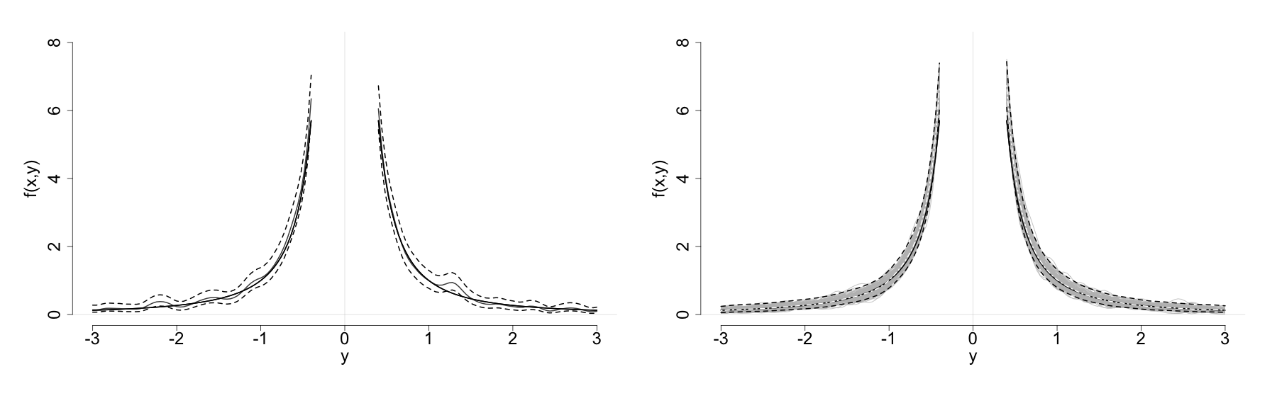
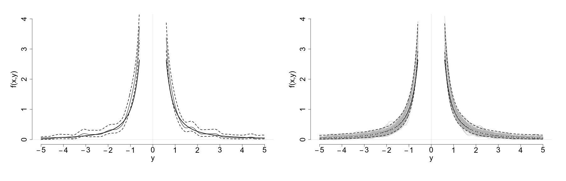
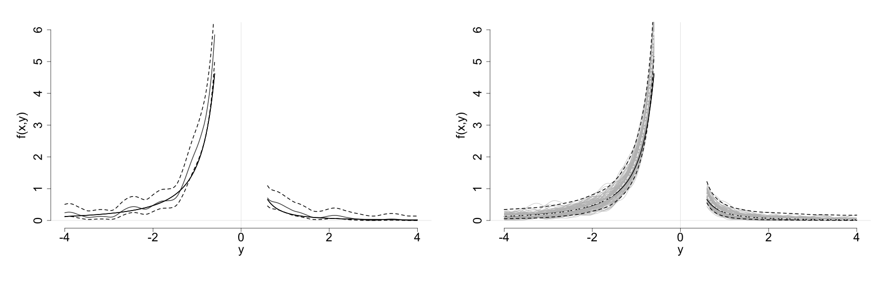
Figure 1: Scenario d3 — Estimation of the Lévy density $f(x,y)$ given by eq. B.1 at $x=0$ with $\eta=(0.4,0.2)$ (top row), at $x=0$ with $\eta=(0.2,0.4)$ (middle row), and at $x=2$ with $\eta=(0.2,0.4)$ (bottom row) based on discrete observations with lag $\Delta=0.0025$ up to time $n\Delta=2500$. Left: One typical estimate (grey) is compared to the true Lévy density (black). The upper and lower bounds of the estimated (pointwise) 95% -confidence intervals (dashed lines) are shown. Right: Estimates based on 100 trajectories (grey) are compared to the true Lévy density (black). The (pointwise) mean of the estimates (white dashed/dotted line) and mean of the upper and lower bounds of the 95% -confidence intervals (black dashed lines) are shown.

References

• Azéma et al. (1967) Azéma, J., Kaplan-Duflo, M., and Revuz, D. (1967) Measure invariante sur les classes recurrents des processus de Markov. Z. Wahrscheinlichkeitstheorie und Verw. Gebiete, 8:157–181.
• Bass (1979) Bass, R. F. (1979) Adding and subtracting jumps from Markov processes. Trans. Amer. Math. Soc., 255:363–376.
• Benveniste and Jacod (1973) Benveniste, A. and Jacod, J. (1973) Systèmes de Lévy des processus de Markov. Invent. Math., 21:183–198.
• Comte and Genon-Catalot (2011) Comte, F. and Genon-Catalot, V. (2011) Estimation for Lévy processes from high frequency data within a long time interval. Ann. Statist., 39:803–837.
• Darling and Kac (1957) Darling, D. A. and Kac, M. (1957) On occupation times for Markoff processes. Trans. Amer. Math. Soc., 84:444–458.
• Down et al. (1995) Down, D., Meyn, S. P., and Tweedie, R. L. (1995) Exponential and uniform ergodicity of Markov processes. Ann. Appl. Probab., 23:1671–1691.
• Fan and Yim (2004) Fan, J. and Yim, T. H. (2004) A crossvalidation method for estimating conditional densities. Biometrika, 91:819–834.
• Figueroa-López (2011) Figueroa-López, J. E. (2011) Sieve-based confidence intervals and bands for Lévy densities. Bernoulli, 17:643–670.
• Getoor (1975) Getoor, R. K. (1975) Markov Processes: Ray Processes and Right Processes, Lecture Notes in Mathematics, vol. 440. Springer, Berlin.
• Greenwood and Wefelmeyer (1994) Greenwood, P. E. and Wefelmeyer, W. (1994) Nonparametric estimators for Markov step processes. Stochastic Process. Appl., 52:1–16.
• Gugushvili et al. (2010) Gugushvili, S., Klaassen, C. A. J., and Spreij, P. (eds.) (2010) Special Issue: Statistical Inference for Lévy Processes with Applications to Finance, Stat. Neerl., vol. 64. Pp. 255–366.
• Hall et al. (2004) Hall, P., Racine, J., and Li, Q. (2004) Cross-validation and the estimation of conditional probability densities. J. Amer. Statist. Assoc., 99:1015–1026.
• Hansen (2009) Hansen, B. E. (2009) Lecture notes on nonparametrics (Spring 2009, Chapters 1–2). Available at http://www.ssc.wisc.edu/~bhansen/718/NonParametrics1.pdf.
• Höpfner (1993) Höpfner, R. (1993) Asymptotic inference for Markov step processes: Observation up to a random time. Stochastic Process. Appl., 48:295–310.
• Höpfner et al. (1990) Höpfner, R., Jacod, J., and Ladelli, L. (1990) Local asymptotic normality and mixed normality for Markov statistical models. Probab. Theory Related Fields, 86:105–129.
• Höpfner and Löcherbach (2003) Höpfner, R. and Löcherbach, E. (2003) Limit theorems for null recurrent Markov processes. Mem. Amer. Math. Soc., 161:vi+92.
• Jacod and Protter (2012) Jacod, J. and Protter, P. (2012) Discretization of Processes. Springer, 2012 edn.
• Jacod and Shiryaev (2003) Jacod, J. and Shiryaev, A. N. (2003) Limit Theorems for Stochastic Processes. Springer, Berlin. 2nd edition.
• Karlsen and Tjøstheim (2001) Karlsen, H. A. and Tjøstheim, D. (2001) Nonparametric estimation in null recurrent time series. Ann. Statist., 29:372–416.
• Löcherbach and Loukianova (2008) Löcherbach, E. and Loukianova, D. (2008) On Nummelin splitting for continuous time Harris recurrent Markov processes and applications to kernel estimation for multi-dimensional diffusions. Stochastic Process. Appl., 118:1301–1321.
• Meyn and Tweedie (1993a) Meyn, S. P. and Tweedie, R. L. (1993a) Markov Chains and Stochastic Stability. Springer, London. Online edition, 2005. Available at http://probability.ca/MT/.
• Meyn and Tweedie (1993b) — (1993b) Stability of Markovian processes III: Foster–Lyapunov criteria for continuous-time processes. Adv. Appl. Probability, 25:518–548.
• Neumann and Reiß (2009) Neumann, M. H. and Reiß, M. (2009) Nonparametric estimation for Lévy processes from low-frequency observations. Bernoulli, 15:223–248.
• Neveu (1972) Neveu, J. (1972) Potentiel markovien récurrent des chaînes de Harris. Ann. Inst. Fourier (Grenoble), 22:85–130.
• Picard (1996) Picard, J. (1996) On the existence of smooth densities for jump processes. Probab. Theory Relat. Fields, 105:481–511.
• Renyi (1963) Renyi, A. (1963) On stable sequences of events. Sankhyā Ser. A, 25:293–302.
• Sawyer (1970) Sawyer, S. A. (1970) A formula for semigroups, with an application to branching diffusion processes. Trans. Amer. Math. Soc., 152:1–38.
• Touati (1987) Touati, A. (1987) Théorèmes limites pour des processus de Markov récurrents. C. R. Acad. Sci. Paris Sér. I Math., 305:841–844.
• Ueltzhöfer (2013) Ueltzhöfer, F. A. J. (2013) On the estimation of jumps of continuous-time stochastic processes. Ph.D. thesis, Technische Universität München.
• Ueltzhöfer and Klüppelberg (2011) Ueltzhöfer, F. A. J. and Klüppelberg, C. (2011) An oracle inequality for penalised projection estimation of Lévy densities from high-frequency observations. J. Nonparametr. Stat., 23:967–989.
• Watanabe (1964) Watanabe, S. (1964) On discontinuous additive functionals and Lévy measures of a Markov process. Japan. J. Math., 34:53–70.
• Weil (1971) Weil, M. (1971) Conditionnement par rapport au passé strict. Séminaire de Probabiltés (Strasbourg), 5:362–372.
Refer to caption
Refer to caption
Refer to caption