Non-ideal MHD Properties of Magnetic Flux Tubes in the Solar Photosphere

Abstract

Magnetic flux tubes reaching from the solar convective zone into the chromosphere have to pass through the relatively cool, and therefore non-ideal (i.e. resistive) photospheric region enclosed between the highly ideal sub-photospheric and chromospheric plasma. It is shown that stationary MHD equilibria of magnetic flux tubes which pass through this region require an inflow of photospheric material into the flux tube and a deviation from iso-rotation along the tube axis. This means that there is a difference in angular velocity of the plasma flow inside the tube below and above the non-ideal region. Both effects increase with decreasing cross section of the tube. Although for characteristic parameters of thick flux tubes the effect is negligible, a scaling law indicates its importance for small-scale structures. The relevance of this “inflow effect” for the expansion of flux tubes above the photosphere is discussed.

MHDmagnetohydrodynamics, ODEordinary differential equation, rhsright hand side

1 Introduction

The interaction of solar flux tubes with the surrounding plasma is usually treated in the framework of ideal MHD (i.e. with zero resistivity), in which no exchange of plasma between the flux tube and its environment is possible. While this approach appears to be well suited for both the convection zone and the upper chromosphere (where the degree of ionisation is sufficiently high), it becomes doubtful for the relatively cold and therefore almost neutral photospheric plasma (see Figure 4). It this resistive layer, deviations from the rigid coupling between fluid and field must be anticipated. This could have important consequences for the widely used conception of flux tubes being wound up by photospheric motions. Also the strict separation of plasma within the flux tube from its environment as required in ideal MHD might break down in this resistive layer. The purpose of this work is to compute this deviation from ideal MHD in a self-consistent manner.
First we consider a stationary magnetic flux tube with both ends anchored in the convective zone (see Figure 2a). The flux tube can be thought of as consisting of a set of nested tubes which are flux surfaces for the magnetic field. Assigning to each of these surfaces the magnetic flux it encloses defines a function $\Psi({\bf r})$, ${\bf B}({\bf r})\cdot\nabla\Psi=0$, which is zero on the tube axis and monotonously increases outwards. (We assume that there are no field reversals within the flux tube.) In a stationary situation, any ideal MHD flow has to preserve these flux surfaces, and the plasma velocity has to be tangential to the surfaces of constant $\Psi$, ${\bf v}\cdot\nabla\Psi=0$. The lower boundary of the domain under consideration (given by the lower boundary of the photosphere) is a surface which intersects the flux tube twice. Any plasma motion imposed on the boundary at one footpoint implies a corresponding motion at the other footpoint. The exact relation between these motions is derived from “ideal” Ohm’s law (i.e. as it is known from ideal MHD)

$$-\nabla\Phi+{\bf v}\times{\bf B}=0\ .$$ (1)

At the lower boundary, the plasma velocity and the magnetic field may be decomposed into their poloidal and toroidal components:

$${\bf v}={\bf v}_{\rm t}+{\bf v}_{\rm p}\quad\mbox{and}\quad{\bf B}={\bf B}_{\rm t}+{\bf B}_{\rm p}\ .$$ (2)

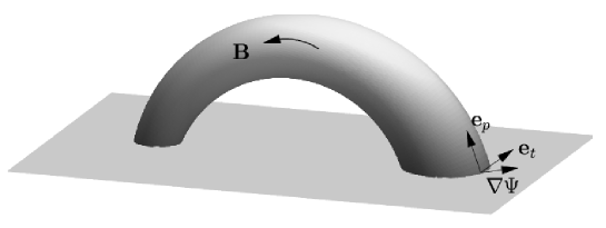
Figure 1: Orientation of unit vectors ${\bf e}_{\rm p}$ and ${\bf e}_{\rm t}$ with respect to the tube surface and the lower photospheric boundary.

The toroidal components are directed along the intersection of the boundary surface with the $\Psi$-surfaces of the flux tube. Their orientation can be defined by requiring that the toroidal unit vector ${\bf e}_{\rm t}$ have a positive orientation with respect to the magnetic field vector on the tube axis. The poloidal components are also tangential to the $\Psi$ surfaces but perpendicular to ${\bf e}_{\rm t}$, with a unit vector ${\bf e}_{\rm p}:=\nabla\Psi\times{\bf e}_{\rm t}\ /\ \|\nabla\Psi\|$ (see Figure 1). Assuming ${\bf v}_{\rm p}={\bf 0}$ and using ${\bf B}_{\rm p}=b_{\rm p}\nabla\Psi\times{\bf e}_{\rm t}$ and ${\bf v}_{\rm t}=v_{\rm t}\ {\bf e}_{\rm t}$, Equation (1) yields

$$\nabla\Phi = {\bf v}_{\rm t}\times{\bf B}_{\rm p}=v_{\rm t}\ b_{\rm p}\ \nabla\Psi$$ (3)

$$\Rightarrow\quad v_{\rm t} = \frac{1}{b_{\rm p}}\frac{\partial\Phi}{\partial\Psi}$$ (4)

since (3) implies $\Phi=\Phi(\Psi)$. This equation shows that a given $v_{\rm t}$ distribution at one end of the flux tube determines ${\partial\Phi}/{\partial\Psi}$, a function which depends only on $\Psi$ and is thus constant along the flux surfaces, thereby inducing a corresponding $v_{\rm t}$ distribution at the other end. For a flux tube which is perpendicular to the boundary and which has circular flux surfaces $\Psi=\Psi(r)$ (where $r$ is the distance from the tube axis), the poloidal component of ${\bf B}$ is given by ${\bf B}_{\rm p}=1/(2\pi r)\ \nabla\Psi(r)\times{\bf e}_{\rm t}$ and hence $b_{\rm p}=1/(2\pi r)$. In this case $v_{\rm t}$ and the angular velocity $\omega:=v_{\rm t}/r$ are functions of $r$ only, i.e. they are constant on each flux surface $\Psi$. This is simply Ferraro’s law of iso-rotation [Moffat (1978)]. In the general case $v_{\rm t}$ is not constant on flux surfaces, but an integration along ${\bf e}_{\rm t}$ yields the circulation time

$$T(\Psi)=\oint{\frac{{\rm d}l}{v_{\rm t}}}=\left(\frac{\partial\Phi}{\partial\Psi}\right)^{-1}\oint b_{\rm p}\ {\rm d}l$$ (5)

which only depends on the flux surface. This quantity (or the corresponding angular velocity $\Omega=2\pi/T$) explicitly shows the coupling of the toroidal velocity field between both ends of the flux tube.
While the preceding results were based on the idealness of the plasma, we will now investigate the effect of a non-ideal region the flux tube has to pass. This non-ideal region is given by the comparatively cold photosphere. Here a possible slippage effect due to the non-ideal photospheric region would result in a deviation of $v_{\rm p}$ from (4). Also in the case of incompatible poloidal velocities on both footpoints the onset of slippage will keep the resulting twist of the flux tube finite, as opposed to the infinite “winding-up” of field lines expected for ideal MHD.

2 The model

To study the effect of a resistive layer on the flux tube, it is sufficient to consider only one half of the tube and concentrate on the photospheric region close to the footpoint, as shown in Figure 2a. For simplicity, we will restrict ourselves to stationary, axisymmetric solutions. The ensuing calculations will use cylindrical coordinates $[r,\phi,z]$, with unit vectors $[{\bf e}_{r},{\bf e}_{\phi},{\bf e}_{z}]$. The $(z=0)$–plane is given by the photosphere’s lower boundary, while the $z$–axis coincides with the tube axis and is pointing away from the Sun. The problem’s axial symmetry is now conveniently incorporated by setting $\partial_{\phi}=0$. With $\partial_{t}=0$, the set of MHD equations to be solved for the mass flow velocity v and the fields B and ${\bf E}=-\nabla\Phi$ consists of the momentum balance (6), a resistive Ohm’s law (7), the equation of continuity (8), and the remaining Maxwell equations (9, 10):

$${\bf 0} = -\nabla P+{\bf j\times B}+\rho\ {\bf g}$$ (6)

$$\eta\ \bf j = -\nabla\Phi+\bf v\times{\bf B}$$ (7)

$$0 = \nabla\cdot(\rho\ {\bf v})$$ (8)

$$\mu\ {\bf j} = \nabla\times{\bf B}$$ (9)

$$0 = \bf\nabla\cdot{\bf B}$$ (10)

As usual, $\rho$ and $\eta$ denote the plasma’s mass density and resistivity, respectively. The inertia term $\rho({\bf v}\cdot\nabla){\bf v}$ is omitted from (6) since its ratio to the induction term ${\bf j\times B}$ is of order ${\cal O}[(v/v_{\rm A})^{2}]$, where

$$v_{\rm A}:=B/\sqrt{\mu\ \rho}$$ (11)

is the Alfvén velocity. Adopting $B\approx$ 0.1 T and $\rho\approx 10^{-6}$ kg m^-3 as characteristic values for our photospheric flux tube yields $v_{\rm A}\approx$ 90 km s^-1, which is large compared to the magnitude of observed photospheric plasma motions of $v_{\rm obs}\approx$ 5 km s^-1. Section 6.3 gives an a posteriori verification of this conjecture.

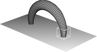
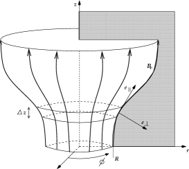
Figure 2 a. Figure 2 b.

Figure 2: Left: Flux tube emerging from the Sun’s photosphere. The white box marks the section on which our computations focus. Right: Our flux tube model. The shaded area indicates the poloidal plane in which ${\bf B}_{\rm p}$, ${\bf v}_{\perp}$ and ${\bf e}_{\parallel,\perp}$ are located.

3 Resistive Inflow

3.1 Derivation of the Inflow Equation

An important difference between the ideal and the non-ideal case is the exchange of plasma between the flux tube and its environment, a process which is impossible in ideal MHD. The plasma flow across the flux surfaces of the magnetic field can be derived from Ohm’s law (7) alone

$$-\nabla\Phi+{\bf v\times B}={\hat{\eta}}\ \nabla\times{\bf B}$$ (12)

with (9) inserted and ${\hat{\eta}}:=\eta/\mu$ substituted. Again we decompose v and B similar to (2) into their toroidal and poloidal components, where the toroidal component is directed along ${\bf e}_{\phi}$ and the poloidal plane is the $r-z$-plane. This yields, after insertion into (12),

$${\bf v}_{\rm p}\times{\bf B}_{\rm p}={\hat{\eta}}\ \nabla\times{\bf B}_{\rm p}$$ (13)

as the poloidal component of Equation (12). Now let

$${\bf e}_{\parallel}:=\frac{1}{B_{\rm p}}\ {\bf B}_{\rm p}\\ \qquad\mbox{and}\qquad{\bf e}_{\perp}:={\bf e}_{\rm t}\times{\bf e}_{\parallel}$$ (14)

be two orthonormal vector fields parallel and perpendicular to ${\bf B}_{\rm p}$. Then the crossproduct of Equation (12) with ${\bf B}_{\rm p}$, together with ${\bf v}_{\rm p}=v_{\perp}{\bf e}_{\perp}+v_{\parallel}{\bf e}_{\parallel}$ yields:

$${\bf B}_{\rm p}\times({\bf v}_{\rm p}\times{\bf B}_{\rm p}) = {\hat{\eta}}\ {\bf B}_{\rm p}\times(\nabla\times{\bf B}_{\rm p})$$

$$\Leftrightarrow\quad B_{\rm p}^{2}\ v_{\perp}\ {\bf e}_{\perp} = {\hat{\eta}}\ {\bf B}_{\rm p}\times\left(\nabla B_{\rm p}\times{\bf e}_{\parallel}+B_{\rm p}\nabla\times{\bf e}_{\parallel}\right)$$

$$\Rightarrow\quad\quad v_{\perp}\ {\bf e}_{\perp} = {\hat{\eta}}\ \left({\bf e}_{\perp}\cdot\nabla(\ln|B_{\rm p}|)-(\nabla\times{\bf e}_{\parallel})\cdot{\bf e}_{\rm t}\right){\bf e}_{\perp}\ .$$ (15)

3.2 Discussion of Inflow Properties

From the “inflow equation” (15), the following flow properties are evident. First, the flow magnitude is proportional to ${\hat{\eta}}$ and thus, as expected, vanishes as soon as ideality is restored. Second, both magnitude and direction of ${\bf B_{\rm p}}$ play no role for ${\bf v}_{\perp}$ or, in other words, a substitution ${\bf B_{\rm p}}\rightarrow\pm\alpha\ {\bf B_{\rm p}}$ leaves ${\bf v}_{\perp}$ unchanged for any constant $\alpha$. (Note that a substitution ${\bf B_{\rm p}}\rightarrow-{\bf B_{\rm p}}$ changes the direction of both ${\bf e}_{\parallel}$ and ${\bf e}_{\perp}$, thereby preserving the direction of ${\bf v}_{\perp}$.)
Moreover, since for a flux tube $B_{\rm p}$ generically decreases outwards, there will generally be an inflow of matter into the tube throughout the entire region where $\eta\neq 0$ due to the first term on the rhs of Equation (15). The contribution of the second term will be negligible in generic cases for the following reason. Both terms define a characteristic length scale. For the first term, this is the scale ${R}$ on which the poloidal field decreases markedly. It can be used for defining the radius of the flux tube as well. The second term defines a typical curvature radius ${R}_{c}$ of the poloidal field lines. If ${R}_{c}$ is of the order of ${R}$, the flux tube is strongly distorted, i.e. the change of its cross section is of the same size as the cross section itself. A closer analysis shows that the field lines of ${\bf B}_{\rm p}$ have to be bent strongly inwards for the second term to contribute to an outward directed flow and to dominate over the first term. (For an instructive example see the Appendix.) However, observational evidence suggests that a flux tube’s cross section either stays more or less constant (Klim,WaKl) or increases monotonously with height, as in sunspots. Noticeable amounts of inward curvature are produced in neither of the two cases, and the second term of (15) can thus be ignored without much loss of generality. (Note that even if such cases should occur, the notion of a tube-shaped configuration requires that strong inward curvature of field lines at one tube part be balanced by a suitably strong outward curvature at some other part. Consequently, the weaker the inflow gets at one point, the stronger it gets at some other point, as can clearly be seen in Figure 8 of the Appendix. Although the fact that the net value of this mutual cancelling of flow depends on the global density structure makes a precise quantitative treatment of the most general case more difficult, it seems reasonable to assume that even then the net inflow will be diminished only moderately by strong poloidal curvature.)
In the case of straight flux tubes, the approximation of small $\nabla\times{\bf e}_{\parallel}$ becomes exact and leads to a scaling of the inflow velocity

$$\|{\bf v}_{\perp}\|\propto 1/{R}\ ,$$ (16)

which means that the inflow is more violent for thinner tubes. For instance, comparing cylindrical flux tubes with the same ${\bf B}_{\rm p}$ profile but different characteristic radii $R$

$${\bf B}_{\rm p}(r)=B_{0}\ b_{z}(r/{R})\ {\bf e}_{z}$$ (17)

we find

$${\bf v}_{\perp}={\hat{\eta}}\ \nabla(\ln|B_{\rm p}|)={\hat{\eta}}\ R^{-1}\ \partial_{x}(\ln|b_{z}(x)|)$$ (18)

where the dimensionless radial coordinate $x:=r/R$ has been introduced. We may thus conclude that the total mass inflow through a cylindrical surface of radius $R$ occurring within the resistive layer,

$$\dot{M} := \int(\rho\ {\bf v}_{\perp})\cdot{\bf da}=\int(\rho\ v_{\perp})\ 2\pi R\ {\rm d}z$$ (19)

$$= \ 2\pi\ \Big{(}\partial_{x}\ \ln|b_{z}(x)|\Big{)}\bigg{|}_{x=1}\int\rho(z)\ {\hat{\eta}(z)}\ {\rm d}z\ ,$$ (20)

is scale-independent with respect to $R$ under the assumption of a horizontally stratified atmosphere ($\rho=\rho(z)$ and ${\hat{\eta}}={\hat{\eta}}(z)$), i.e. tubes of various radii but with the same $b_{z}$ profile will transport the same mass rate, regardless of their strength. (Note that the momentum equation (6) was not used to derive the preceeding results, which therefore are not limited to flow fields satisfying $v\ll v_{A}$.)

4 Solving for the Complete Flow Field

From now on, it will be assumed for simplicity that the tube is of cylindrical shape, i.e. it does not “fan out”. This simplifying assumption is justified by the fact that the main effects of the resistive layer, namely the flow of plasma into the flux tube and the decoupling of toroidal velocities above and below this layer, are both already present in this simplified geometry. Our assumption then translates to $B_{r}(r,z)\equiv 0$, so that the solenoidality condition (10) now reads

$$0=\nabla\cdot{\bf B}=\partial_{z}B_{z}(r,z)\ .$$ (21)

Now consider the momentum equation (6) in its $[r,\phi,z]$ components:

$$\left(\begin{array}[]{c}0\\ 0\\ 0\end{array}\right)=-\left(\begin{array}[]{c}\partial_{r}P(r,z)\\ 0\\ \partial_{z}P(r,z)\end{array}\right)+{\bf j}\times{\bf B}+\rho(r,z)\left(\begin{array}[]{c}0\\ 0\\ -g\end{array}\right)$$ (22)

From the $\phi$-component we derive $\partial_{z}B_{\phi}(r,z)=0$ and hence ${\bf B}={\bf B}(r)$, such that we can integrate the pressure from the $r$-component of (22)

$$P(r,z)=p_{1}(r)+p_{2}(z)\ ,$$ (23)

which in turn leads to $\partial_{r}\rho(r,z)=0$ due to the $z$-component of (22). Assuming that $P$, $\rho$ and $T$ are linked by an arbitrary equation of state $P=P[\rho,T]$, a horizontally stratified temperature $T(z)$ yields $\partial_{r}P(r,z)\equiv 0$ and hence

$${\bf j}\times{\bf B}\equiv{\bf 0}\ .$$ (24)

Therefore a cylindrical flux tube has to be force-free if the temperature of the plasma is horizontally stratified.
Although the requirement of strictly horizontal isotherms $T=T(z)$ is clearly not fulfilled for very thick tubes (as readily seen by the reduced intensity observed in sunspots), we choose to adhere to this assumption not only for the benefits of a markedly simplified analytical treatment but also for physical reasons. Setting $\partial_{r}T=0$ would be justified provided that sufficiently strong horizontal heat transport was present. However, under the assumption of an ideal plasma, the (radiation-dominated) influx of heat does not suffice to heat the interior of an embedded flux tube to the ambient temperature level because convective energy transport is inhibited by the tube’s strong magnetic field, as was first realised by Bier. But within the non-ideal zone, convection across magnetic surfaces is well permitted (or even enforced, see Section 3), such that the radial exchange of heat will be amplified significantly. The inflow effect thus reduces the radial temperature gradient and may possibly lead to thermal structures with $\partial_{r}T\ll\partial_{z}T$, in which case our assumption would be clearly justified. (This condition should be easily fulfilled for thin tubes, while thick tubes will hardly be affected by this reasoning since it takes too long to exchange noticeable fractions of their mass contents via the inflow effect, see Section 6.2.) Moreover, the presence of neutral gas in this region allows for additional convective energy transport unimpeded by magnetic fields.
In our case, the only non-trivial component of (24) is the $r$-component, which reduces to

$$\partial_{x}\left(b_{z}^{2}(x)+b_{\phi}^{2}(x)\right)+2\ b_{\phi}^{2}(x)/x=0\ ,$$ (25)

where again $x\equiv r/R$, $b_{\phi}(x):=B_{\phi}(xR)/B_{0}$, and $b_{z}(x):=B_{z}(xR)/B_{0}$ were used. This equation is solved by

$$b_{\phi}^{2}(x)=-x\ \partial_{x}G(x)\quad\mbox{and}\quad b_{z}^{2}(x)=(1/x)\ \partial_{x}[x^{2}G(x)]$$ (26)

for any function $G(x)$ satisfying $\partial_{x}G(x)<0$ and $\partial_{x}[x^{2}G(x)]>0$ [Schlüter (1957)]. Figure 3 shows a typical solution to (25).

Figure 3: Selected field lines of $\displaystyle(b_{\phi},b_{z})=\left(x/(1+x^{2}),1/(1+x^{2})\right)$, which satisfies (25) and corresponds to $G(x)=[2(1+x^{2})]^{-1}$.

Given a force-free magnetic field, the solution for the flow velocity ${\bf v}$ is to be determined from Ohm’s law and the equation of continuity. This also requires to fix boundary conditions for the velocity on either the upper or the lower boundary of the domain. Here the linearity of the two equations with respect to ${\bf v}$ is very useful because any solution can be seen as a superposition of a solution ${\bf v}_{\rm id}$ of the ideal Ohm’s law (1) and the continuity equation, and a particular solution ${\bf v}_{\rm res}$ of the resistive Ohm’s law (7) and the continuity equation:

$${\bf v}={\bf v}_{\rm id}+{\bf v}_{\rm res}\ .$$ (27)

Since we are interested in the deviation from iso-rotation due to the resistive photospheric layer, we are free to determine ${\bf v}_{\rm res}$ for a certain choice of boundary conditions, and the solution for any other boundary condition is then given by adding a corresponding ideal solution. The most simple boundary condition is setting ${\bf v}={\bf 0}$ on the upper boundary $z=z_{\rm up}$, such that the velocity on the lower boundary exactly equals the difference of the toroidal velocities above and below the photosphere, i.e. the deviation from iso-rotation. In this case we have (the index “res” on the solution is suppressed in the following):

$$\begin{array}[]{rrrl}v_{r}(x,z)&=&-R^{-1}&\beta_{1}(x)\ \eta(z)\\ v_{\phi}(x,z)&=&\pm R^{-2}&\big{[}\ \beta_{2}(x)\ I_{2}(z)+\beta_{3}(x)\ I_{1}(z)\ \big{]}\\ v_{z}(x,z)&=&+R^{-2}&\beta_{4}(x)\ I_{2}(z)\end{array}$$ (28)

where the $\beta_{1...4}(x)$ are given by

$$\beta_{1}(x) := \frac{b_{z}^{\prime}(x)}{b_{z}(x)}$$ (29)

$$\beta_{2}(x) := \frac{b_{\phi}(x)}{b_{z}(x)}\left[\frac{b_{z}^{\prime\prime}(x)}{b_{z}(x)}+\frac{1}{x}\frac{b_{z}^{\prime}(x)}{b_{z}(x)}-\left(\frac{b_{z}^{\prime}(x)}{b_{z}(x)}\right)^{2}\right]$$ (30)

$$\beta_{3}(x) := \frac{b_{\phi}(x)}{b_{z}(x)}\left[\frac{b_{z}^{\prime\prime}(x)}{b_{z}(x)}-\left(\frac{b_{z}^{\prime}(x)}{b_{z}(x)}\right)^{2}+\frac{1}{x^{2}}\right]+$$

$$+ \frac{b_{\phi}^{\prime}(x)}{b_{z}(x)}\left[\frac{b_{z}^{\prime}(x)}{b_{z}(x)}-\frac{b_{\phi}^{\prime\prime}(x)}{b_{\phi}^{\prime}(x)}-\frac{1}{x}\right]$$

$$\beta_{4}(x) := \frac{b_{z}^{\prime\prime}(x)}{b_{z}(x)}+\frac{1}{x}\frac{b_{z}^{\prime}(x)}{b_{z}(x)}-\left(\frac{b_{z}^{\prime}(x)}{b_{z}(x)}\right)^{2}$$ (32)

and the $I_{1,2}(z)$ are defined as

$$I_{1}(z):=\int_{z}^{z_{\rm up}}\eta(\zeta)\ {\rm d}\zeta\quad\mbox{and}\quad I_{2}(z):=\int_{z}^{z_{\rm up}}\eta(\zeta)\ \frac{\rho(\zeta)}{\rho(z)}\ {\rm d}\zeta\ .$$ (33)

The sign of $v_{\phi}(x,z)$ in (28) is opposite to the sign of $b_{\phi}(x)$, which is not fixed by (25) and may be chosen arbitrarily. (Figure 3 has sgn $b_{\phi}=+1$.)
To proceed further, one could either prescribe a vortex at $z=0$ and use (25) and (28) to compute the magnetic field components, or insert into (28) a typical solution of (25). The first alternative would use a (rather long and messy) first order ODE, while in the latter case the flow field could be read off directly from (28). Therefore, this avenue is chosen here.

5 Realistic Input Parameters

For a quantitative evaluation, prescription of density and resistivity profiles $\rho(z)$ and $\eta(z)$ is required. We use the data provided by the solar atmosphere model “C” of Vern (hereafter VAL, see Figure 4) along with the conductivity calculations by KuKa based on the VAL model. Since this model neglects magnetic forces, we continue to assume isotropic resistivity for both simplicity and consistency, that is, we take $\eta\equiv(\sigma_{\parallel})^{-1}$ from Table III in [Kubát and Karlický (1985)] (see Figure 5). The function

$$\eta(z)=\eta_{0}\ \left[1+\left(\frac{z-z_{\rm m}}{L_{\eta}}\right)^{4}\right]^{-1}$$ (34)

with [$\eta_{0}=0.058\ \Omega$ m, $z_{\rm m}=360$ km, $L_{\eta}=330$ km] also depicted there will be used to model the photosphere’s actual resistivity; its density is approximated by

$$\rho(z)=\rho_{0}\ \exp(-z/L_{\rho})$$ (35)

with $\rho_{0}=3\cdot 10^{-4}\ {\rm kg\ m^{-3}}$ and $L_{\rho}=120\ {\rm km}$, which is in sufficient agreement with the VAL model data for $\rho(z)$.

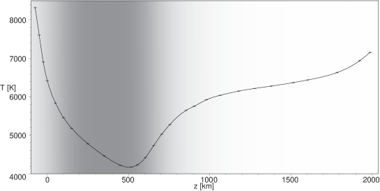
Figure 4: Temperature variation with height according to the VAL model. The shaded area marks the resistive region, in which the ionisation ratio drops below $10^{-5}$. The minimum of $T(z)$ at $z\approx$ 500 km is clearly discernible.

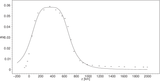
Figure 5: Computed resistivity profile (crosses) vs. analytic model function. The relatively poor agreement between relation (34) and the data at $z<0$ is of minor importance since these layers are not explicitly considered here.

In the ensuing quantifications, we will specialise to the B field of Figure 3 as a “flux tube prototype”. This seems justified since tentative computations using other fields have yielded only very small deviations. Additionally, $z_{\rm up}\rightarrow\infty$ is used since above the non-ideal region the contribution to (33) becomes negligible.

6 Quantitative Flow Evaluation

6.1 The Scaling Law

According to (28), there must be a tube radius $R_{\rm tr.}$ such that

$$v\equiv\|{\bf v}\|\propto\left\{\begin{array}[]{ccc}R^{-1}&:&R\gg R_{\rm tr.}\\ R^{-2}&:&R\ll R_{\rm tr.}\end{array}\right.$$ (36)

Inserting our parameters found in the preceeding section, we find $R_{\rm tr.}\approx$ 5000 km. Since at this radius $v$ will have dropped below 1 m s^-1, we may safely regard

$$\|{\bf v}\|\propto R^{-2}$$ (37)

as the relevant scaling law for small scale flux tubes.

6.2 The Blowup Timescale

The knowledge of absolute photospheric density and resistivity allows us to quantify the total mass inflow (19) associated with a cylindrical tube as $\dot{M}\approx 1.9\cdot 10^{8}$ kg s^-1, which, when compared to the total mass

$$M_{\rm tot}:=\int_{r<R}\rho\ {\rm d}V=\pi R^{2}\int_{0}^{z_{\rm up}}\rho(z)\ {\rm d}z\approx 4.9\cdot 10^{13}\ {\rm kg}\left(\frac{R}{100\ {\rm km}}\right)^{2}$$ (38)

of the plasma contained inside the tube, defines a typical timescale

$$\tau_{\rm blowup}:=\frac{M_{\rm tot}}{\dot{M}}=\frac{R^{2}}{2}\ \frac{\displaystyle\int_{0}^{z_{\rm up}}\rho(z)\ {\rm d}z}{\displaystyle\int_{0}^{z_{\rm up}}\rho(z)\ {\hat{\eta}}(z)\ {\rm d}z}\approx 70\ {\rm h}\left(\frac{R}{100\ {\rm km}}\right)^{2}$$ (39)

at which the tube exchanges a noticeable fraction of its contents.

6.3 Condition for sub-Alfvénic Flows

Since the flow magnitude scales $\propto R^{-2}$, the requirement $v\ll v_{\rm A}$ is actually a limitation on the radius of the flux tube. According to Figure 6, this may be quantified as $R\gsim 10$ km, which is well below the resolvable scale achieved by present (and near-future) solar observations. Discarding the inertia term in (6) was indeed justified.

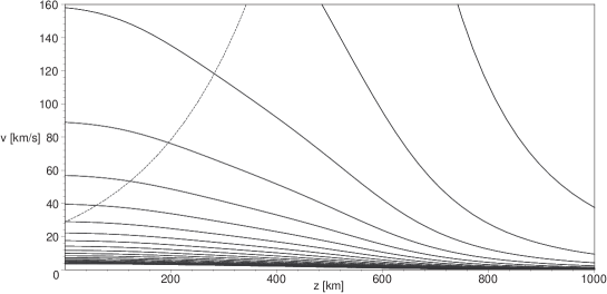
Figure 6: Maximum flow magnitude for tube radii $R\in\{1,2,...20\ {\rm km}\}$ (solid) vs. Alfvén speed (dashed). $v_{\rm A}$ increases $\propto[\rho(z)]^{-1/2}$, i.e. exponentially.

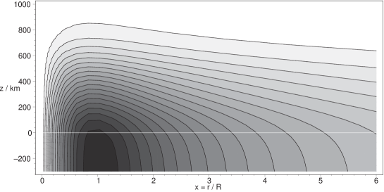
Figure 7: Poloidal contour plot of $v_{\phi}(x,z)$.

6.4 Field Line Slippage

The toroidal flow depicted in Figure 7 shows a striking deviation from the flow expected in the ideal case $\eta=0$ (in which Ferrano’s theorem of iso-rotation forces all field lines to rotate with constant angular velocity $\Omega(x,z):=v_{\phi}(x,z)/(xR)$, such that $\partial_{z}\Omega\equiv 0$). Note also that far below the photosphere ($z<0$), the lines of constant $v_{\phi}$ tend to become vertical, implying that iso-rotation is recovered as $\eta$ again tends to zero.
Since we have $I_{2}(0)/I_{1}(0)\approx 0.1\ll 1$, the profile of the footpoint vortex (i.e. the cut along $z=0$) can be approximated by

$$\frac{v_{\phi}(x,0)}{130\ {\rm m\ s^{-1}}}\approx\left(\frac{R}{100\ {\rm km}}\right)^{-2}\frac{x}{1+x^{2}}\ .$$ (40)

With $\Omega(x,z_{\rm up})=0$, the total difference in angular velocity below and above the non-ideal layer is given by

$$\Delta\Omega(x) := \frac{|v_{\phi}(x,0)|}{xR}\approx\frac{4}{R^{3}}\ \frac{1}{1+x^{2}}\ \int_{0}^{z_{\rm up}}{\hat{\eta}}(\zeta)\ {\rm d}\zeta$$ (41)

$$< \Delta\Omega(0)\approx 3.1\cdot 10^{-4}\ {\rm s}^{-1}\ [R/(100\ \rm km)]^{-3}\ .$$ (42)

For observable tube sizes ($R\gsim 100\ {\rm km}$) this would require a velocity resolution close to $(\Delta v)_{\rm reso}:=R\ \Delta\Omega\approx 30\ {\rm m\ s^{-1}}$. Although this limit is not quite reached by current imaging techniques, the further improvement in image resolution may soon render observational verification feasible.

7 Implications for the Tube’s Global Evolution

Since, according to our results, plasma has to flow into the tube from both ends and cannot leave the tube outside the non-ideal zone, the question arises as to where the inflowing matter goes. The possibilities are a) a steady increase of the tube’s volume (tube gets “inflated”), b) tube is static and downflow into the convection zone occurs or c) the inflowing plasma recombines within the flux tube and leaves the tube in the form of neutral gas. (Of course, in reality various combinations of a) to c) are conceivable.) In the present model, the direction of vertical flow inside the tube is determined by the boundary condition at $z=z_{\rm up}$ (or any other height), such that up- or downflows of arbitrary magnitude can be achieved by choosing a correspondingly large (possibly negative-valued) profile for $x\mapsto v_{z}(x,z_{\rm up})$. However, we have no reason to favour any specific profile, and thus our present, rather simple model cannot provide a definitive answer here. (Note that in Section 4, ${\bf v}|_{z_{\rm up}}={\bf 0}$ (implying downflow at $z=0$) was merely chosen to simplify the calculation of field line slippage. It was not supposed to indicate a preference for downflows in any way.) To shed light on this important issue, the aforementioned possibilities a) to c) suggest two avenues for an extension of our model. First, if plasma was flowing up the tube, thereby forcing it to expand in length and/or cross section, the tube’s field lines would be stretched, and their tension increased. Eventually, the growing contribution from the ${\bf j\times B}$ force might become strong enough to balance the gas pressure, causing the upflow to cease. To see whether such a final equilibrium state exists, and if so, what the tube parameters in such a state are, one would need to abandon cylindrical symmetry and model the full arch-shaped tube such that all effects of field line curvature could properly be accounted for. Unfortunately, the corresponding set of equations could turn out to be very difficult to solve analytically, and thus the feasibility of this approach is unclear at the moment.
Second, evaluating the significance of possibility c) would obviously require the introduction of radial gradients of ionisation and temperature. In such a model, one-dimensional reference atmospheres such as VAL can no longer be used to prescribe atmospheric parameters (except at large distances from the tube axis), and self-consistent modelling of density and temperature becomes mandatory. Again, it seems doubtful whether analytic solutions can be obtained at a reasonable expenditure.
Still, in both cases a recourse to numerical investigations of the described settings remains a vital option and may help to clarify the role of the inflow effect with respect to the tube’s global temporal evolution. (A discussion of observational evidence for downflow is given by Frut, but whether these observations can be applied to the photospheric region remains unclear since they refer to velocities measured at coronal or transition region temperatures. Generally speaking, the very existence of pronounced vertical flows inside photospheric flux tubes still seems to be a controversial issue among the observing community.)

8 Summary

Our analytic investigation of stationary MHD equilibria of magnetic flux tubes has shown that Ohm’s law enforces an inflow of fluid towards loci of higher field strength, which depends neither on the tube’s cross section, nor on the strength and direction of its B field. Being proportional to $\eta$, this inflow occurs wherever the tube penetrates the cool photospheric layer, in particular at the tube’s footpoints.
It was shown that a static flux tube of cylindrical shape has to be force-free if the ambient plasma temperature is horizontally stratified, a result which holds for arbitrary values of plasma beta. The introduction of a resistive layer allows for stationary MHD solutions with finite field twist and a difference in the rotational velocity above and below this resistive layer. This constitutes a marked deviation from the iso-rotational behaviour known from ideal MHD and limits the winding-up of the flux tube’s field lines if incompatible rotational velocities are imposed on the tube’s footpoints. Although according to the scaling law for the plasma flows these effects either too small or too slow to be detected by present solar observations (i.e. the effect either requires too small structures or produces velocities below the detection threshold), a future improvement of observational resolution may soon show whether the described effects can be distinguished from the convective motions of the ambient plasma.

To clarify some aspects concerning the direction of radial flow, consider the magnetic field

$${\bf B}_{\rm sp}:=\frac{B_{0}\ \cosh z}{1+(r\ \cosh z)^{2}}\bigg{(}-r\ \sinh z,\ 0,\ \cosh z\bigg{)}$$ (43)

where the $r$ and $z$ coordinates are now dimensionless for simplicity of the argument. The tube radii have a $(\cosh\ z)^{-1}$ profile and the field decays as $\|{\bf B}_{\rm sp}\|_{z=0}\propto 1/(1+r^{2})$. Figure 8 shows a vector plot of the corresponding perpendicular flow component ${\bf v}_{\perp}$. Beyond the dotted line, the field curvature gets so strong that the flow direction is indeed reversed, leading to an outflow of plasma. Although the existence of photospheric fields like (43) cannot be ruled out completely, the rather low astrophysical significance of such configurations (as discussed in Section 3.2) is further diminished by the fact that ${\bf B}_{\rm sp}$ has $\nabla\times({\bf j\times B})_{\rm sp}\neq{\bf 0}$ and therefore does not describe a flux tube in the hydrodynamical sense.

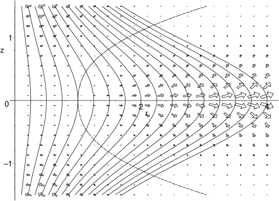
Figure 8: Vector field plot of ${\bf v}_{\perp}$ and selected field lines of B (solid) in the poloidal plane. The flow direction reverses at the dashed line. Note how high curvature increases both inflow (due to the “inflow effect”) and outflow (due to the requirement that the tube be void of field line reversals).