Statistical Multiresolution Estimation for Variational Imaging: With an Application in Poisson-Biophotonics

Abstract.

In this paper we present a spatially-adaptive method for image reconstruction that is based on the concept of statistical multiresolution estimation as introduced in [19]. It constitutes a variational regularization technique that uses an $\ell_{\infty}$-type distance measure as data-fidelity combined with a convex cost functional. The resulting convex optimization problem is approached by a combination of an inexact alternating direction method of multipliers and Dykstra’s projection algorithm. We describe a novel method for balancing data-fit and regularity that is fully automatic and allows for a sound statistical interpretation. The performance of our estimation approach is studied for various problems in imaging. Among others, this includes deconvolution problems that arise in Poisson nanoscale fluorescence microscopy.

1. Introduction

In this paper we are concerned with the reconstruction of an unknown gray-valued image $u^{0}\in\text{L}^{2}(\Omega)$ with $\Omega=[0,1]^{2}$ given the data

$$Y_{ij}=(Ku^{0})_{ij}+\varepsilon_{ij},\quad 1\leq i\leq m,1\leq j\leq n.$$ (1)

For the moment, we assume that $\varepsilon_{ij}$ are independent and identically distributed Gaussian random variables with $\mathbf{E}\left(\varepsilon_{11}\right)=0$ and $\mathbf{E}\left(\varepsilon_{11}^{2}\right)=\sigma^{2}>0$ and that $K:\text{L}^{2}(\Omega)\rightarrow\mathbb{R}^{m\times n}$ is a linear and bounded operator. $K$ is assumed to model image acquisition and sampling at the same time, i.e. $(Ku)_{ij}$ is assumed to be a sample at the pixel $(i/m,j/n)$ of a smoothed version of $u$. Throughout the paper we will assume that $\sigma^{2}$ is known (for reliable estimation techniques for $\sigma^{2}$ see e.g. [30] and references therein).

A popular approach for computing a stable approximation of $u^{0}$ from the data $Y$ given in the Gaussian model (1) consists in minimizing the penalized least squares functional, i.e.

$$\hat{u}(\lambda)\in\operatorname*{\textnormal{argmin}}_{u\in\text{L}^{2}(\Omega)}\frac{\lambda}{2}\sum_{i,j}\left|(Ku)_{ij}-Y_{ij}\right|^{2}+J(u)$$ (2)

where $J:\text{L}^{2}(\Omega)\rightarrow\overline{\mathbb{R}}$ is a convex and lower-semicontinuous regularization functional and $\lambda>0$ a suitable multiplier. In the seminal work [33], for example, the authors proposed the total variation semi-norm

$$J(u)=\begin{cases}\left|\text{D}u\right|(\Omega)&\text{ if }u\in\text{BV}(\Omega)\\ +\infty&\text{ else}\end{cases}$$ (3)

as a penalization functional which has been a widely used model in imaging ever since. Here, $\left|\text{D}u\right|(\Omega)$ denotes the total variation of the (measure-valued) gradient of $u$ which coincides with $\int_{\Omega}\left|\nabla u\right|$ if $u$ is smooth. Numerous efficient solution methods for (6) [7, 10, 26] and various modifications have been suggested so far (cf. [8, 20, 31, 36] to name but a few). In particular, in order to accelerate numerical algorithms and to prevent oversmoothing the total variation semi-norm is often augmented to

$$J(u)+\gamma\int_{\Omega}u^{2}$$ (4)

with $\gamma\geq 0$.

The quadratic fidelity in (2) has an essential drawback: The information in the residual is incorporated globally, that is each pixel value $(Ku)_{ij}-Y_{ij}$ contributes equally to the estimator $\hat{u}(\lambda)$ independent of its spatial position. In practical situations this is clearly undesirable, since images usually contain features of different scales and modality, i.e. constant and smooth portions as well as oscillating patterns both of different spatial extent. A solution $\hat{u}(\lambda)$ of (2) is hence likely to exhibit under- and oversmoothed regions at the same time.

Recently, spatially-adaptive reconstruction approaches became popular that are based on (2) with a locally varying regularization parameter, i.e.

$$\hat{u}(\lambda)\in\operatorname*{\textnormal{argmin}}_{u\in\text{L}^{2}(\Omega)}\frac{1}{2}\sum_{i,j}\lambda_{ij}\left|(Ku)_{ij}-Y_{ij}\right|^{2}+J(u).$$ (5)

However, the choice of the multiplier function $\lambda_{ij}$ is subtle and different approaches have been suggested. See for instance [21, 22, 11, 27].

In this paper we take a different route to achieve spatial adaption which allows to “localize” any convex functional $J$ by minimizing it over a convex set that is determined by the statistical extreme value behaviour of the residual process. More precisely, we study estimators $\hat{u}$ of $u^{0}$ that are computed as solutions of the convex optimization problem

$$\inf_{u\in\text{L}^{2}(\Omega)}J(u)\quad\text{ s.t. }\quad\max_{S\in\mathcal{S}}\frac{c_{S}}{\sigma^{2}}\sum_{(i,j)\in S}\left|(Ku)_{ij}-Y_{ij}\right|^{2}\leq 1.$$ (6)

Here, $\mathcal{S}$ denotes a system of subsets of the grid $G=\left\{1,\ldots,m\right\}\times\left\{1,\ldots,n\right\}$ and $\left\{c_{S}~{}:~{}S\in\mathcal{S}\right\}$ is a set of positive weights that govern the trade-off between data-fit and regularity locally on each set $S\in\mathcal{S}$. Solutions of (6) are special instances of statistical multiresolution estimators (SMRE) as studied in [19]. In this context the statistic $T:\mathbb{R}^{m\times n}\rightarrow\mathbb{R}$ defined by

$$T(v)=\max_{S\in\mathcal{S}}\frac{c_{S}}{\sigma^{2}}\sum_{(i,j)\in S}\left|v_{ij}\right|^{2},\quad v\in\mathbb{R}^{m\times n}$$ (7)

is referred to as multiresolution (MR) statistic. Summarizing, an SMRE $\hat{u}$ of $u^{0}$ is an element with minimal $J$ among all candidate estimators $u$ that satisfy the condition $T(Ku-Y)\leq 1$.

Special instances of (6) have been studied recently: For the case when $\mathcal{S}$ contains the entire domain $G$ only, it has been shown in [8] that (6) is equivalent to (2) if $K$ satisfies certain conditions. As mentioned above, this approach is likely to oversmooth small-scaled image features (such as texture) and/or underregularize smooth parts of the image. An improved model was proposed in [2] where $\mathcal{S}$ is chosen to consist of a (data-dependent) partition of $G$ that is obtained in a preprocessing step (for the numerical simulations in [2], Mumford-Shah segmentation is considered). Under similar conditions on $K$ as in [8], it was shown in [2] that (6) is equivalent to (5) where $\lambda_{ij}$ is constant on each $S\in\mathcal{S}$. This approach was further developed in [1] where a subset $S\subset G$ is fixed and afterwards $\mathcal{S}$ is defined to be the collection of all translates of $S$ (in fact, the authors study the convolution of the squared residuals with a discrete kernel). The authors propose a proximal point method for the solution of (6). This approach of local constraints w.r.t. a window (or kernel) of fixed size was also studied in [15] for irregular sampling and regularization functionals other than the total variation were considered. In particular, it is observed that the difference between results obtained by using the total variation penalty (3) and the Dirichlet-energy (integrated squared norm of the derivative) is not so big when using local constraints. This is in accordance to findings in [18] for one-dimensional signals. In [11] the model of [1] was studied in the continuous function space setting. Moreover the authors in [11] provided a fast algorithm for the solution of the constrained optimization problem based on the hierarchical decomposition scheme [34] combined with the unconstrained problem (5).

In this paper, we propose a novel, automatic selection rule for the weights $c_{S}$ based on a statistically sound method that is applicable for any pre-specified, deterministic system of subsets $\mathcal{S}$. We are particularly interested in the case when $\mathcal{S}$ constitutes a highly redundant collection of subsets of $G$ consisting of overlapping subsets of different scales. This is a substantial extension to the approaches in [1, 15, 11] that only consider one fixed (pre-defined) scale. Our approach will amount to select a single parameter $\alpha\in[0,1]$ with the interpretation that the true signal $u^{0}$ satisfies the constraint in (6) with probability $\alpha$. From the definition of (6) it is then readily seen that $\mathbb{P}\left(J(\hat{u})\leq J(u^{0})\right)\geq\alpha$ for any solution $\hat{u}$ of (6). In other words, our method controls the probability that the reconstruction $\hat{u}$ is at least as smooth (in the sense of $J$) as the true image $u^{0}$. To this aim, it will be necessary to gain stochastic control on the null-distribution $T(\varepsilon)$, where $\varepsilon=\left\{\varepsilon_{ij}\right\}$ is a lattice of independent $\mathcal{N}(0,\sigma^{2})$- distributed random variabels.

Moreover, for the efficient solution of (6) we extend the algorithmic ideas in [19] and propose a combination of an inexact alternating direction method of multipliers (ADMM) [13, 9] with Dykstra’s projection algorithm [4]. Finally, we indicate how our approach can be applied to image deblurring problems in fluorescence microscopy where the observed data does not fit into the white noise model (1) but where one usually assumes that independently

$$Y_{ij}\sim\textnormal{Pois}\left((Ku)_{ij}\right),\quad 1\leq i\leq m,1\leq j\leq n$$ (8)

Here, $\textnormal{Pois}(\beta)$ stands for the Poisson distribution with parameter $\beta>0$. We mention that similar models occur in positron emission tomography (cf. [35]) and large binocular telescopes (cf. [3]) and we claim that our method can be useful there as well. We apply Anscombe’s transform to transform the Poisson data to normality. Furthermore we present a modified version of the ADMM to solve the resulting variant of (6). We finally illustrate the capability of our approach by numerical examples: Image denoising, deblurring and inpainting and deconvolution problems that arise in nanoscale fluorescence microscopy.

In the following, we denote by $\left|S\right|$ the cardinality of $S\in\mathcal{S}$. We often refer to $\left|S\right|$ as the scale of $S$. We assume that $m,n\in\mathbb{N}$ are fixed and denote by $\left\langle\cdot,\cdot\right\rangle$ and $\left\|\cdot\right\|$ the Euclidean inner-product and norm on $\mathbb{R}^{m\times n}$ and by $\left\|u\right\|_{\text{L}^{2}}$ the $\text{L}^{2}$-norm of $u$. For a convex functional $J:\text{L}^{2}(\Omega)\rightarrow\overline{\mathbb{R}}$ the subdifferential $\partial J(u)$ is the set of all $\xi\in\text{L}^{2}(\Omega)$ such that $J(v)\geq J(u)+\int_{\Omega}\xi(v-u)$ for all $v\in\text{L}^{2}(\Omega)$. The Bregman-distance between $v,u\in\text{L}^{2}(\Omega)$ w.r.t. $\xi\in\partial J(u)$ is defined by

$$D_{J}^{\xi}(v,u)=J(u)-J(v)-\int_{\Omega}\xi(u-v)\geq 0.$$

If additionally $\eta\in\partial J(v)$ we define the symmetric Bregman distance by $D_{J}^{\text{sym}}(u,v)=D_{J}^{\xi}(v,u)+D_{J}^{\eta}(u,v)$. By $J^{*}$ we denote the Legendre-Fenchel transform of $J$, i.e. $J^{*}(q)=\sup_{u\in\text{L}^{2}(\Omega)}\int_{\Omega}uq-J(u)$. We finally note that it would not be restricitve (yet less intuitive) to replace $\text{L}^{2}(\Omega)$ by any other separable Hilbert space.

2. Statistical Multiresolution Estimation

We review sufficient conditions that guarantee existence of SMREs, solutions of (6) that is. To this end, we rewrite (6) into an equality constrained problem and study the corresponding augmented Lagrangian function (Section 2.1). Moreover, we address the important question on how to choose the scale weights $c_{S}$ automatically in Section 2.2. Finally, we discuss different choices for the system $\mathcal{S}$ that have proved feasible in practice in Section 2.3.

2.1. Existence of SMRE

For the time being, let $\left\{c_{S}~{}:~{}S\in\mathcal{S}\right\}$ be a set of positive real numbers. We rewrite (6) to an equality constrained problem by introducing the slack variable $v\in\mathbb{R}^{m\times n}$. To be more precise, we aim for the solution of

$$\inf_{u\in\text{L}^{2}(\Omega),v\in\mathbb{R}^{m\times n}}J(u)+H(v)\quad\text{ s.t. }\quad Ku-v=0$$ (9)

where $H$ denotes the indicator function on the feasible set $\mathcal{C}$ of (6), i.e.

$$\mathcal{C}=\left\{v\in\mathbb{R}^{m\times n}~{}:~{}T(v-Y)\leq 1\right\}\quad\text{ and}\quad H(v)=\begin{cases}0&\text{ if }v\in\mathcal{C}\\ +\infty&\text{ else }\end{cases}.$$ (10)

Problems of type (9) were studied extensively in [16, Chap. III]. There, Lagrangian multiplier methods are employed to solve (9). Recall the definition of the augmented Lagrangian of (9):

$$L_{\lambda}(u,v;p)=\frac{1}{2\lambda}\left\|Ku-v\right\|^{2}+J(u)+H(v)+\left\langle p,Ku-v\right\rangle,\quad\lambda>0.$$ (11)

Here $p\in\mathbb{R}^{m\times n}$ denotes the Lagrange multiplier for the linear constraint in (9). Note that $L_{\lambda}$ equals the ordinary Lagrangian $L(u,v;p)=J(u)+H(v)+\left\langle p,Ku-v\right\rangle$ augmented by the quadratic term $\left\|Ku-v\right\|^{2}/(2\lambda)$ that fosters the fulfillment of the linear constraint in (9).

It is well known that the saddle-points of $L$ and $L_{\lambda}$ coincide (cf. [16, Chap III Thm. 2.1]) and that existence of a saddle point of $L_{\lambda}$ follows from existence of solutions of (9) together with constraint qualifications of the MR-statistic $T$. One typical example for the latter is given in Proposition 2.1. The result is rather standard and can be deduced e.g. from [12, Chap III, Prop 3.1 and Thm. 4.2] (cf. also [16, Chap III])

Proposition 2.1.

Assume that (9) has a solution $(\hat{u},\hat{v})\in\text{L}^{2}(\Omega)\times\mathbb{R}^{m\times n}$ and that there exists $\bar{u}\in\text{L}^{2}(\Omega)$ such that $J(\bar{u})<\infty$ and $T(K\bar{u}-Y)<1$ (Slater’s constraint qualification). Then, there exists $\hat{p}\in\mathbb{R}^{m\times n}$ such that $(\hat{u},\hat{v},\hat{p})$ is a saddle point of $L_{\lambda}$, i.e.

$$L_{\lambda}(\hat{u},\hat{v};p)\leq L_{\lambda}(\hat{u},\hat{v};\hat{p})\leq L_{\lambda}(u,v;\hat{p}),\quad\forall\left(u\in\text{L}^{2}(\Omega),v,p\in\mathbb{R}^{m\times n}\right).$$

Remark 2.2.

1. If $\hat{u}\in\text{L}^{2}(\Omega)$ and $\hat{v},\hat{p}\in\mathbb{R}^{m\times n}$ are as in Proposition 2.1, then $\hat{u}$ is an SMRE, i.e. it solves (6). Moreover, the following extremality relations hold:

   $$-K^{*}\hat{p}\in\partial J(\hat{u}),\quad\hat{p}\in\partial H(\hat{v})\quad\text{ and }\quad K\hat{u}=\hat{v}.$$

2. Slater’s constraint qualification is for instance satisfied if the set

   $$\left\{Ku~{}:~{}u\in\text{L}^{2}(\Omega)\text{ and }J(u)<\infty\right\}$$

   is dense in $\mathbb{R}^{m\times n}$.

3. If $J$ is chosen to be the total variation semi-norm (3), then a sufficient condition for the existence of solutions of (9) will be that there exists $(i,j)\in S$ for some $S\in\mathcal{S}$ such that $(K\mathbf{1})_{ij}\not=0$, where $\mathbf{1}\in\text{L}^{2}(\Omega)$ is the constant $1$-function. This is immediate from Poincaré’s inequality for functions in $\text{BV}(\Omega)$ (cf. [37, Thm.5.11.1]).

2.2. An a priori parameter selection method

The choice of the scale weights $c_{S}$ in (6) is of utmost importance for they determine the trade-off between smoothing and data-fit (and hence play the role of spatially local regularization parameters). We propose a statistical method that is based on quantile values of extremes of transformed $\chi^{2}$ distributions.

We pursue the strategy of controlling the probability that the true signal $u^{0}$ satisfies the constraint in (6). To this end, observe that for $S\in\mathcal{S}$ the random variable

$$t_{S}(\varepsilon)=\sigma^{-2}\sum_{(i,j)\in S}\varepsilon_{ij}^{2}$$

is $\chi^{2}$-distributed with $\left|S\right|$ degrees of freedom (d.o.f.). With this notation, it follows from (1) that $u^{0}$ satisfies the constraints in (6) if

$$T(Ku^{0}-Y)=T(\varepsilon)=\max_{S\in\mathcal{S}}c_{S}t_{S}(\varepsilon)\leq 1.$$

Additionally, we require that the maximum above is balanced in the sense that the probability for $c_{S}t_{S}(\varepsilon)>1$ is equal for each $S\in\mathcal{S}$.

To achieve this, we first aim for transforming $t_{S}(\varepsilon)$ to normality. It was shown in [23] that the fourth root transform $\sqrt[4]{t_{S}(\varepsilon)}$ is approximately normal with mean and variance

$$\mu_{S}=\sqrt[4]{\left|S\right|-0.5}\quad\text{ and }\quad\sigma^{2}_{S}=\left(8\sqrt{\left|S\right|}\right)^{-1},$$

respectively. The fourth root transform outperforms other power transforms in the sense that the Kullback-Leibler distance to the normal distribution is minimized, see [23]. In particular, it was stressed in [23] that the approximation works well for small d.o.f. Next, we consider the extreme value statistic

$$\max_{S\in\mathcal{S}}\frac{\sqrt[4]{t_{S}(\varepsilon)}-\mu_{S}}{\sigma_{S}}.$$ (12)

We note that due to the transformation of the random variable $t_{S}(\varepsilon)$ to normality each scale contributes equally to the supremum in (12). Hence a parameter choice strategy based on quantile values of the statistic (12) is likely to balance the different scales occurring in $\mathcal{S}$. We make this precise in the following

Proposition 2.3.

For $\alpha\in(0,1)$ and $S\in\mathcal{S}$ let $q_{\alpha}$ be the $\alpha$-quantile of the statistic (12) and set $c_{S}=(q_{\alpha}\sigma_{S}+\mu_{S})^{-4}$. Then, any solution $\hat{u}$ of (6) satisfies

$$\mathbb{P}(J(\hat{u})\leq J(u^{0}))\geq\alpha.$$ (13)

Proof.

From (1) and from the monotonicity of the mapping $x\mapsto\sqrt[4]{x}$ it follows that

$$\mathbb{P}\left(T(Ku^{0}-Y)\leq 1\right) = \mathbb{P}\left(c_{S}t_{S}(\varepsilon)\leq 1\;\forall S\in\mathcal{S}\right)$$

$$= \mathbb{P}\left(\sqrt[4]{t_{S}(\varepsilon)}\leq q_{\alpha}\sigma_{S}+\mu_{S}\;\forall S\in\mathcal{S}\right)$$

$$= \mathbb{P}\left(\max_{S\in\mathcal{S}}\frac{\sqrt[4]{t_{S}(\varepsilon)}-\mu_{S}}{\sigma_{S}}\leq q_{\alpha}\right)=\alpha.$$

In other words, the constants $c_{S}$ are chosen such that the true signal $u^{0}$ satisfies the constraints with probability $\alpha$. By the fact that $\hat{u}$ is a solution of (6) it follows that $\mathbb{P}(T(Ku^{0}-Y)\leq 1)\leq\mathbb{P}(J(\hat{u})\leq J(u^{0}))$. ∎

Remark 2.4.

By the rule $c_{S}=(q_{\alpha}\sigma_{S}+\mu_{S})^{-4}$ in Proposition 2.3 the problem of selecting the set of scale weights $c_{S}$ is reduced to the question on how to choose the single value $\alpha\in(0,1)$. The probability $\alpha$ plays the role of an universal regularization parameter and allows for a precise statistical interpretation: It constitutes a lower bound on the probability that the SMRE $\hat{u}$ is more regular (in the sense of $J$) than the true object $u^{0}$. Moreover, one has that

$$c_{S}t_{S}(\varepsilon)>1\quad\Leftrightarrow\quad\frac{\sqrt[4]{t_{S}(\varepsilon)}-\mu_{S}}{\sigma_{S}}>q_{\alpha},\quad\text{ for all }S\in\mathcal{S}.$$

Note, that the constraint in (6) can be rewritten into

$$\frac{1}{\left|S\right|}\sum_{(i,j)\in S}\left|(Ku)_{ij}-Y_{ij}\right|^{2}\leq\frac{\sigma^{2}}{c_{s}\left|S\right|},\quad\text{ for all }S\in\mathcal{S}.$$

Since $\mathbf{E}\left(\left|S\right|^{-1}\sum_{(i,j)\in S}\varepsilon_{ij}^{2}\right)=\sigma^{2}$ and $\mathbf{Var}\left(\left|S\right|^{-1}\sum_{(i,j)\in S}\varepsilon_{ij}^{2}\right)=2\sigma^{4}\left|S\right|^{-1}$ the factor $1/(c_{S}\left|S\right|)$ can be considered as a relaxation parameter, that takes into account the uncertainty of estimating the variance of the residual on finite scales $\left|S\right|$. Put differently, it is expected to be large on small scales and approaches $1$ as $\left|S\right|$ increases. This is illustrated in Figure 1: Here the quantity $1/(c_{S}\left|S\right|)$ is depicted for the system $\mathcal{S}_{0}$ of all squares with sidelengths up to $20$ (left panel) and the system $\mathcal{S}_{2}$ of all dyadic squares (middle panel) in an $341\times 512$ image for $\alpha=0.2$ (’+’) and $\alpha=0.9$ (’o’). It becomes clear, that only on the smallest scales there are non-negligible differences between the scale weights for $\mathcal{S}_{0}$ and $\mathcal{S}_{2}$. Also our numerical experiments confirm, that reconstruction results do not differ very much for different choices of $\alpha$.

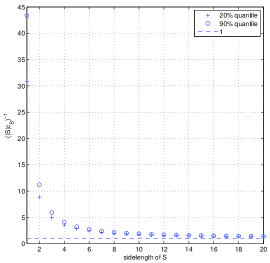
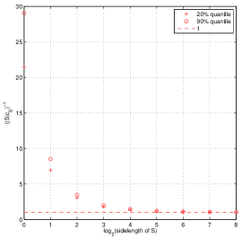
Figure 1. Left and middle: Dependence of relaxation factor $(c_{S}\left|S\right|)^{-1}$ on $\alpha$ and scale $\left|S\right|$. Right: Empirical density of the statistic (12). All values are computed for a $341\times 512$ image and w.r.t. to $\mathcal{S}_{0}$ (solid) and $\mathcal{S}_{2}$ (dashed).

We note that in [1] and [11] the authors propose relaxation parameters for the case when $\mathcal{S}$ consists of the translates of a window of fixed size. In [1] the authors fix such a parameter, $1.01$ say, and determine the corresponding window size by heurisitc reasoning. In [11] the authors give for a fixed window size $\left|S\right|$ a formula for a relaxation parameter that uses moments of the extreme value statistic of independent $\chi^{2}$ random variables with $\left|S\right|$ degrees of freedom. We note that these methods can not be generalized to systems $\mathcal{S}$ that contains sets of different scales case in a straightforward manner. Our selection rule for the weights $c_{S}$ is designed such that different scales are balanced appropriately. Hence our approach is a multi-scale extension of the (single-scale) methods in [1, 11].

Remark 2.5.

It is important to note that the random variable $t_{S}(\varepsilon)$ and $t_{S^{\prime}}(\varepsilon)$ are independent if and only if $S\cap S^{\prime}=\emptyset$. As we do not assume that $\mathcal{S}$ consists of pairwise disjoint sets, (12) constitutes an extreme value statistic of dependent random variables. Except for special cases, little is known about the distribution of such statistics (see e.g. [28, 29] for asymptotic results). It is an open and interesting problem to investigate the asymptotic properties of the distribution of the statistic in (12).

In practice, the quantile values $q_{\alpha}$ in Proposition 2.3 are derived from the empirical distribution of (12). The right panel in Figure 1 shows the empiricial density of the statistic (12) for $m=341$ and $n=512$ and the systems $\mathcal{S}_{0}$ (solid) and $\mathcal{S}_{2}$ (dashed) (for our simulations in Figure 1 we used $5000$ trials).

2.3. On the choice of $\mathcal{S}$

In the previous section we addressed the question on how to select the scale weights $\left\{c_{S}\right\}_{S\in\mathcal{S}}$ for a given system of subsets $\mathcal{S}$ of the grid $G$. Altough it is not the primary aim of this paper to advocate a particular systems $\mathcal{S}$, we will now comment on possible determinants for a rational choice of $\mathcal{S}$.

Figure 2. Left: true signal $u^{0}$. Right: noiys data $Y$ with $\sigma=0.1$

Figure 3. Solution of (2) $\hat{u}(\lambda)$ with $\lambda=0.075$.

On the one hand, $\mathcal{S}$ should be chosen rich enough to resolve local features of the image sufficiently well at various scales. On the other hand, it is desirable to keep the cardinality of $\mathcal{S}$ small such that the optimization problem in (6) remains solvable within reasonable time. As a consequence of this, a priori information on the signal $u^{0}$ should be employed in practice in order to delimit a suitable system $\mathcal{S}$ (e.g. the range of scales to be used). Furthermore we note that for guaranteeing that the extreme value statistic (12) does not degenerate (as $m,n$ and the cardinality of $\mathcal{S}$ increase), $\mathcal{S}$ typically has to satisfy certain entropy conditions (see e.g. [18]). We stress that it is a challenging and interesting task to extend these results to random (data-driven) systems $\mathcal{S}$. It is well known that such methods can yield good results in practice (see e.g. [2]).

Here, we discuss two different choices of $\mathcal{S}$, namely:

1. the set of all discrete squares in $G$: for computational reasons usually subsystems are considered. We found the subset consisting of all squares with sidelengths up to $20$ to be efficient. We denote this subset henceforth by $\mathcal{S}_{0}$.

2. the set $\mathcal{S}_{2}$ of dyadic partitions of $G$. For a quadratic grid $G$ with $m=n=2^{r}$ the system $\mathcal{S}_{2}$ is obtained by recursively splitting the grid into four equal squares until the lowest level of single pixels is reached. To be more precise,

   $$\mathcal{S}_{2}=\bigcup_{l=1}^{r}\left\{\left\{k2^{l},\ldots,(k+1)2^{l}\right\}^{2}~{}:~{}k=0,\ldots,2^{r-1}\right\}.$$

   For general grids $G$ the left and lower most squares are clipped accordingly.

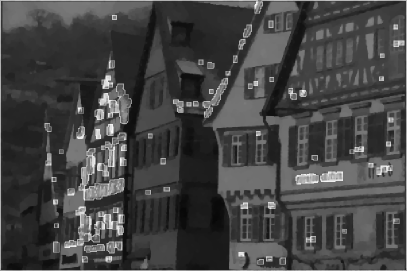
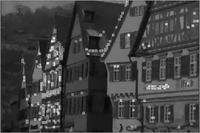
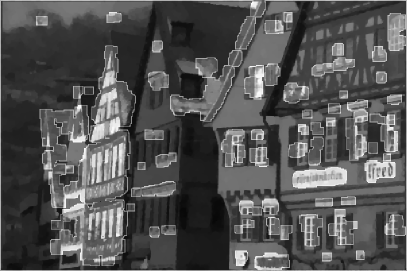
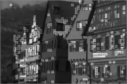
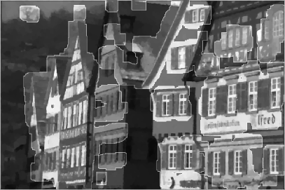
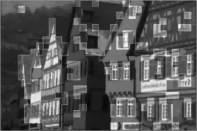
Figure 4. Oversmoothed regions identified on the scales $\left|S\right|=4,8$ and $16$ (from left to right) for the system $\mathcal{S}_{0}$ (left column) and $\mathcal{S}_{2}$ (right column).

Obviously, $\mathcal{S}_{0}$ contains much more elements than $\mathcal{S}_{2}$ and is hence likely to achieve a higher resolution. We indicate this by a numerical simulation. Figure 2 depicts the true signal $u^{0}$ (left, at a resolution of $m\times n=341\times 512$ pixels and gray values scaled in $[0,1]$) and data $Y$ according to (1) with $K=\textnormal{Id}$ and $\sigma=0.1$.

For illustrative purpose a global estimator $\hat{u}(\lambda)$ in (2) for $u^{0}$ is computed that exhibits both over- and undersmoothed regions (here, we set $\lambda=0.075$). This estimator is depicted in Figure 3. The oversmoothed parts in $\hat{u}(\lambda)$ can be identified via the MR-statistic $T$ in (7) by marking those sets $S$ in $\mathcal{S}$ for which

$$\frac{c_{S}}{\sigma^{2}}\sum_{(i,j)\in S}\left|Y_{ij}-(K\hat{u}(\lambda))_{ij}\right|^{2}>1.$$

The union of these sets for the systems $S_{0}$ (left column) and $S_{2}$ (right column) are highlighted in Figure 4 where we examine the scales $\left|S\right|=4,8,16$. The parameters $c_{S}$ are chosen as in Section 2.2 with $\alpha=0.9$.

3. Algorithmic Methodology

In what follows, we present an algorithmic approach to the numerical computation of SMRE in practice that extends the methodology in [19] where we proposed an alternating direction method of multipliers (ADMM). Here, we use an inexact version of the ADMM which decomposes the original problem into a series of subproblems which are substantially easier to solve. In particular, an inversion of the operator $K$ is no longer necessary. For this reason the inexact ADMM has attracted much attention recently (see. e.g. [9, 14, 36]).

3.1. Inexact ADMM

In order to compute the desired saddle point of the augmented Lagrangian function $L_{\lambda}$ in (11), we use the inexact ADMM that can be considered as a modified version of the Uzawa algorithm (see e.g. [16, Chap. III]). Starting with some initial $p_{0}\in\mathbb{R}^{m\times n}$, the original Uzawa algorithm consists in iteratively computing

1. $(u_{k},v_{k})\in\operatorname*{\textnormal{argmin}}_{u\in\text{L}^{2}(\Omega),v\in\mathbb{R}^{m\times n}}L_{\lambda}(u,v;p_{k-1})$

2. $p_{k}=p_{k-1}+\lambda(Ku_{k}-v_{k})$.

Item $(1)$ amounts to an implicit minimization step w.r.t. to the variabels $u$ and $v$ whereas $(2)$ constitutes an explicit maximization step for the Lagrange multiplier $p$. The algorithm is usually stopped once the constraint in (9) is fulfilled up to a certain tolerance.

Applying this algorithm in a straightforward manner is known to be rather impractical (mostly due to the difficult minimization problem in the first step) and hence various modifications have been proposed in the optimization literature. Firstly, we perform successive minimization w.r.t. $u$ and $v$ instead of minimizing simultaneously, i.e. given $(u_{k-1},v_{k-1},p_{k-1})$ we compute

1. $u_{k}\in\operatorname*{\textnormal{argmin}}_{u\in\text{L}^{2}(\Omega)}L_{\lambda}(u,v_{k-1};p_{k-1})$

2. $v_{k}\in\operatorname*{\textnormal{argmin}}_{v\in\mathbb{R}^{m\times n}}L_{\lambda}(u_{k},v;p_{k-1})$

3. $p_{k}=p_{k-1}+\lambda(Ku_{k}-v_{k})$.

This is the well-known alternating direction method of multipliers (ADMM) as proposed in [16, Chap. III]). There, convergence of the algorithm has been studied for the case when $J$ satisfies some regularity assumptions. In [19] we extended this result for general functionals $J$ (as for example the total variation semi-norm (3)). The resulting two minimization problems usually can be tackled much more efficiently than the original problem.

Still, the first subproblem above requires the inversion of the (possibly ill-posed) operator $K$. Thus, a second modification adds in the $k$-th loop of the algorithm the following additional term to $L_{\lambda}(u,v_{k-1};p_{k-1})$:

$$\frac{1}{2\lambda}\left(\zeta\left\|u-u_{k-1}\right\|^{2}_{\text{L}^{2}}-\left\|K(u-u_{k-1})\right\|^{2}\right).$$ (14)

Here, $\zeta$ is chosen such that $\zeta>\left\|K\right\|^{2}$. After some rearrangements of the terms in $L_{\lambda}$ and (14) it can easily be seen that $Ku$ cancels out and thus the undesirable inversion of $K$ is is replaced by a single evaluation of $K$ at the previous iterate $u_{k-1}$. However, by adding (14) the distance to the previous iterate $u_{k-1}$ is additionally penalized and $L_{\lambda}(u,v_{k};p_{k-1})$ is minimized only inexactly.

After the aforementioned rearrangements and by keeping in mind that $H$ is the indicator function of the convex set $\mathcal{C}$ in (10), the inexact ADMM can be summarized as follows:

Algorithm 1 Inexact ADMM

0:  $Y\in\mathbb{R}^{m\times n}$ (data), $\lambda>0$ (step size).

  $u_{0}\leftarrow\vec{0}_{\text{L}^{2}}$ and $v_{0}=p_{0}\leftarrow 0$.

  for $k=1,2,\ldots$ do

     $k\leftarrow k+1$.

     Minimize $L_{\lambda}(\cdot,v_{k-1};p_{k-1})+\frac{1}{2\lambda}\left(\zeta\left\|\cdot-u_{k-1}\right\|^{2}_{\text{L}^{2}}-\left\|K(\cdot-u_{k-1})\right\|^{2}\right)$:

$$u_{k}\leftarrow\operatorname*{\textnormal{argmin}}_{u\in\text{L}^{2}(\Omega)}\frac{1}{2}\left\|u-\left(u_{k-1}-\zeta^{-1}K^{*}(Ku_{k-1}-v_{k-1}+\lambda p_{k-1}\right)\right\|_{\text{L}^{2}}^{2}+\frac{\lambda}{\zeta}J(u).$$ (15)

     Minimize $L_{\lambda}(u_{k},\cdot;p_{k-1})$:

$$v_{k}\leftarrow\operatorname*{\text{proj}}_{\mathcal{C}}\left(Ku_{k}+\lambda p_{k-1}\right).$$ (16)

     Update dual variable:

$$p_{k}\leftarrow p_{k-1}+\lambda^{-1}(Ku_{k}-v_{k}).$$ (17)

  end for

In practice, Algorithm 1 is very stable and straightforward to implement, provided that efficient methods to solve (15) and (16) are at hand (cf. Section 3.2 below). Moreover, it is equivalent to a general first-order primal-dual algorithm as studied in [9] where the following convergence result was established.

Theorem 3.1.

[9, Thm. 1] Assume that $(\hat{u},\hat{v},\hat{p})$ is a saddle point of $L_{\lambda}$. Moreover, let $\left\{u_{k},v_{k},p_{k})\right\}_{k\in\mathbb{N}}$ be generated by Algorithm 1 with $\zeta>\left\|K\right\|^{2}$ and define the averaged sequences

$$\bar{u}_{k}=\frac{1}{k}\sum_{l=1}^{k}u_{l}\quad\text{ and }\quad\bar{p}_{k}=\frac{1}{k}\sum_{l=1}^{k}p_{l}.$$

Then, each weak cluster point of $\left\{\bar{u}_{k}\right\}_{k\in\mathbb{N}}$ is a solution of (6) and there exists a constant $C>0$ such that

$$D_{J}^{-K^{*}\hat{p}}(\bar{u}_{k},\hat{u})+D_{H^{*}}^{\hat{v}}(\bar{p}_{k},\hat{p})\leq C/k.$$ (18)

The above result is rather general and in particular situations the assertions may be quite weak. In particular if $J$ and $H^{*}$ have linear growth, as it is for instance the case for $J$ as in (3) and $H$ as in (10), the Bregman distances appearing in (18) may vanish although $(\bar{u}_{k},\bar{p}_{k})\not=(\hat{u},\hat{p})$. If at least one of the functionals $J$ or $H^{*}$ is uniformly convex, it is possible to come up with accelerated versions of Algorithm 1 that allow for stronger convergence results (see [9]). For the sake of simplicity we restrict our consideration to the basic algorithm.

3.2. Subproblems

Closer inspection of Algorithm 1 reveals that the original problem - computing a saddle point of $L_{\lambda}$ - has been replaced by an iterative series of subproblems (15) and (16). We will now examine these two subproblems and propose methods that are suited to solve them. Here we proceed as in [19].

We focus on (16) first. Note that the problem given there amounts to computing the orthogonal projection of $v_{k}:=Ku_{k}+\lambda p_{k-1}$ onto the feasible region $\mathcal{C}$ as defined in (10). Due to the supremum taken in the definition (7) of the statistic $T$, we can decompose $\mathcal{C}$ into $\mathcal{C}=\bigcap_{S\in\mathcal{S}}\mathcal{C}_{S}$ where

$$\mathcal{C}_{S}=\left\{v\in\mathbb{R}^{m\times n}~{}:~{}\frac{c_{S}}{\sigma^{2}}\sum_{(i,j)\in S}\left|v_{ij}-Y_{ij}\right|^{2}\leq 1\right\},$$ (19)

i.e. each $\mathcal{C}_{S}$ refers to the feasible region that would result if $\mathcal{S}$ contained $S$ only. Note that all $\mathcal{C}_{S}$ are closed and convex sets (in fact, they are circular cylinders in $\mathbb{R}^{m\times n}$; see the left panel in Figure 5). If we fix a $\mathcal{C}_{S}$ and consider some $v\notin\mathcal{C}_{S}$, the projection of $v$ onto $\mathcal{C}_{S}$ can be stated explicitly as

$$(P_{\mathcal{C}_{S}}(v))_{i,j}=\begin{cases}v_{i,j}\quad&\text{if}\quad(i,j)\notin S\\ \left.Y_{ij}+(v_{ij}-Y_{ij})\sigma\middle/\sqrt{c_{S}\sum_{(k,l)\in S}(v_{kl}-Y_{kl})^{2}}\right.\quad&\text{if}\quad(i,j)\in S.\\ \end{cases}$$ (20)

This insight leads us to the conclusion that any method which computes the projection onto the intersection of closed and convex sets by merely using the projections onto the individual sets only would be feasible to solve (16). Dykstra’s Algorithm [4] works exactly in this way and is hence our method of choice to solve (16). For a detailed statement of the algorithm and how the total number of sets that enter it may be decreased to speed up runtimes, see [19, Sec. 2.3]. We note that despite these considerations, the predominant part of the computation time of Algorithm 1 is spent for the projection step (16). So far we did not take into account parallelization of the projection algorithm. To some extent this is possible in a straightforward manner, since the projections onto disjoint sets in $\mathcal{S}$ can be carried out simultaneously (on GPUs for instance). But also inherently parallel projection algorithms (including parallel versions of Dykstra’s method) received much attention recently and potentially would yield a speed up of Algorithm 1. See for instance [6] for an overview.

We finally turn our attention to (15). In contrast to the standard version of the ADMM as proposed in [19], the second subproblem in Algorithm 1 does not involve the inversion of the operator $K$. For this reason, (15) here simply amounts to solving an unconstrained denoising problem with a least-squares data-fit. Numerous methods for a wide range of different choices of $J$ are available in order to cope with this problem. If $J$ is chosen as the total variation seminorm, for example, the methods introduced in [7, 10, 26] will be suited (we will use the one in [10]).

4. Application in Fluorescence Microscopy

For image acquisition techniques that are based on single photon counts of a light emitting sample, such as fluorescence microscopy, the Gaussian error assumption (1) is not realistic. Here, the non-additive model (8) is to be preferred. Still, the estimation paradigm above can be adapted to this scenario by means of variance stabilizing transformations. To this end we first recall [5, Lem. 1]

Lemma 4.1 (Anscombe’s Transform).

Let $Y\sim\textnormal{Pois}(\beta)$ with $\beta>0$. Then, for all $c\geq 0$

$$\mathbf{E}\left(2\sqrt{Y+c}\right) =2\sqrt{\beta}+\frac{4c-1}{4\sqrt{\beta}}+\mathcal{O}(\beta^{-3/2})$$

$$\mathbf{Var}\left(2\sqrt{Y+c}\right) =1+\frac{3-8c}{8\beta}+\mathcal{O}(\beta^{-2}).$$

Thus, the choice $c=3/8$ is likely to stabilize the variance of $2\sqrt{Y+c}$ at the constant value $1$ (in second order) and its mean at $2\sqrt{\beta}$ (in first order) or in other words it approximately holds that

$$2\sqrt{Y+3/8}-2\sqrt{\beta}\sim\mathcal{N}(0,1).$$

It is obvious from Lemma 4.1 that the choice $c=1/4$ will result in a better reduction of the bias, since the mean is then stabilized at $2\sqrt{\beta}$ in second order (at the cost of a less stable variance). Numerically, we found the difference to be negligible for our purposes.

With the above considerations, it is straightforward to adapt the estimation scheme (6) to the present case: Let $X_{ij}=2\sqrt{Y_{ij}+3/8}$. Then, we define a statistical multiresolution estimator $\hat{u}$ for the model (8) to be any solution of

$$\inf_{u\in\text{L}^{2}(\Omega)}J(u)\quad\text{ s.t. }\quad \sup_{S\in\mathcal{S}}c_{S}\sum_{(i,j)\in S}\left|X_{ij}-2\sqrt{(Ku)_{ij}}\right|^{2}\leq 1,$$ (21)

$$(Ku)_{ij}\geq 0,\quad\text{ for all }(i,j)\in G.$$

Note that for any $c>0$ the function $t\mapsto(\sqrt{t}-c)^{2}$ is convex on $[0,\infty)$ and thus Problem (21) is again a convex optimization problem. Similar as in Section 2.1 we can rewrite (21) into

$$\inf_{u\in\text{L}^{2}(\Omega),v\in\mathbb{R}^{m\times n}}J(u)+\tilde{H}(v)\quad\text{ s.t. }\quad Ku-v=0,$$ (22)

where here $\tilde{H}$ denotes the indicator function on the feasibility set $\tilde{\mathcal{C}}$ given by

$$\tilde{\mathcal{C}}=\left\{v\in\mathbb{R}^{m\times n}~{}:~{}v_{ij}\geq 0\text{ for all }(i,j)\in G\text{ and }T(2\sqrt{v}-X)\leq 1\right\}.$$ (23)

\psfrag{y1}{$Y_{1}$}\psfrag{y2}{$Y_{2}$}\psfrag{5}{$5$}\psfrag{10}{$10$}\psfrag{v1}{$v_{1}$}\psfrag{v2}{$v_{2}$}\includegraphics[width=195.12767pt]{admiss_gauss}

\psfrag{y1}{$Y_{1}$}\psfrag{y2}{$Y_{2}$}\psfrag{5}{$5$}\psfrag{10}{$10$}\psfrag{v1}{$v_{1}$}\psfrag{v2}{$v_{2}$}\includegraphics[width=195.12767pt]{admiss_poiss}

Figure 5. Admissible domains for $1\times 2$ “images” and data $Y_{1}=(1,1)$ and $Y_{2}=(7,4)$: Left: the sets $\mathcal{C}$ for the Gaussian case with $\sigma^{2}=1$ (cf. (10)). Right: the sets $\tilde{\mathcal{C}}$ for the Poisson case (cf. (23)). The scale weights $c_{S}$ are chosen as proposed in Proposition 2.3 with $\alpha=0.9$. The gray lines delimit the sets $\mathcal{C}_{S}$ and $\tilde{\mathcal{C}}_{S}$ for $S\in\mathcal{S}=\left\{(1,0),(0,1),(1,1)\right\}$.

The right panel in Figure 5 depicts the sets $\tilde{\mathcal{C}}$ for the simple case $m=2$ and $n=1$. It is important to note, that in contrast to the Gaussian case (left panel), the feasibility sets $\tilde{C}$ are not translation invariant, i.e. their shape and size depend on the data $Y$. In particular, the size increases with $\left\|Y\right\|$ which is due to the fact that the variance of a Poisson random variable with law $\text{Pois}(\beta)$ increases linearly with the parameter $\beta$.

In principle, Algorithm 1 can be directly applied to solve (21): The set $\mathcal{C}$ in the projection step (17) has to be replaced by the modified feasibility set $\tilde{\mathcal{C}}$. Again, we observe that $\tilde{\mathcal{C}}=\bigcap_{S\in\mathcal{S}}\tilde{\mathcal{C}}_{S}$, where

$$\tilde{\mathcal{C}}_{S}=\left\{v\in\mathbb{R}_{\geq 0}^{m\times n}~{}:~{}c_{S}\sum_{(i,j)\in S}\left|2\sqrt{v_{ij}}-X_{ij}\right|^{2}\leq 1\right\}.$$

Using Dykstra’s Algorithm amounts to compute the orthogonal projections onto the sets $\tilde{\mathcal{C}}_{S}$ which, in contrast to the Gaussian case, is no longer possible in closed form (except for the case when $\left|S\right|=1$) and approximate solutions have to be used. Since during the runtime of Algorithm 1 these projections are to be computed a considerable amount of time, this is clearly undesirable since inevitable numerical errors are likely to accumulate.

As a way out, assume for the time being, that $\hat{y}\in\mathbb{R}^{m\times n}$ is some estimator for $\sqrt{Ku^{0}}$ with $\hat{y}_{ij}>0$. Then, by Taylor expansion, we find for $u\in\text{L}^{2}(\Omega)$ that

$$2\sqrt{(Ku)_{ij}}=\hat{y}_{ij}+\frac{(Ku)_{ij}}{\hat{y}_{ij}}+\mathcal{O}(\left|\hat{y}_{ij}^{2}-(Ku)_{ij}\right|^{2}).$$

In place of (21), we propose to solve the linearized problem

$$\inf_{u\in\text{L}^{2}(\Omega)}J(u)\quad\text{ s.t. }\quad \sup_{S\in\mathcal{S}}c_{S}\sum_{(i,j)\in S}\left|X_{ij}-\hat{y}_{ij}-(Ku)_{ij}/\hat{y}_{ij}\right|^{2}\leq 1,$$ (24)

$$(Ku)_{ij}\geq 0,\quad\text{ for all }(i,j)\in G.$$

Similar as above, we rewrite (24) into

$$\inf_{u\in\text{L}^{2}(\Omega),w\in\mathbb{R}^{m\times n}}J(u)+H_{\hat{y}}(w)\quad\text{ s.t. }\quad\frac{Ku}{\hat{y}}-w=0.$$

where $H_{\hat{y}}$ is the indicator function on the feasible set $\mathcal{C}_{\hat{y}}$ given by

$$\mathcal{C}_{\hat{y}}=\left\{w\in\mathbb{R}^{m\times n}~{}:~{}w_{ij}\geq 0\text{ for all }(i,j)\in G\text{ and }T(w+\hat{y}-X)\leq 1\right\}$$

Clearly, the orthogonal projection onto $\mathcal{C}_{\hat{y}}$ can again be computed efficiently by Dykstra’s algorithm as outlined in Section 3. The corresponding augmented Lagrangian functional reads as

$$L_{\lambda,\hat{y}}(u,w;p)=\frac{1}{2\lambda}\left\|Ku/\hat{y}-w\right\|^{2}+J(u)+H_{\hat{y}}(w)+\left\langle p,Ku/\hat{y}-w\right\rangle.$$ (25)

For any “good” estimator $\hat{y}$ for $\sqrt{Ku^{0}}$ Algorithm 1 could be applied immediately to find a saddle point $(\hat{u},\hat{w},\hat{p})$ of $L_{\lambda,\hat{y}}$, but usually such an estimator is not at hand. We hence propose to replace in the $k$-th loop of Algorithm 1 the estimator $\hat{y}$ by $\sqrt{Ku_{k}}$. To avoid instabilities we rather use $\sqrt{\max(Ku_{k},\delta)}$ for some small positive parameter $\delta>0$. We formalize these ideas in Algorithm 2.

Algorithm 2 ADMM for Poisson Noise

0:  $Y\in\mathbb{R}^{m\times n}$ (data), $\lambda>0$ (step size), $\delta>0$.

  $w_{0}=p_{0}\leftarrow 0$ and init $y_{0}\in\mathbb{R}_{>0}^{m\times n}$.

  for $k=1,2,\ldots$ do

     $k\leftarrow k+1$.

     Minimize $L_{\lambda,w_{k-1}}(\cdot,w_{k-1};p_{k-1})$:

$$u_{k}\leftarrow\operatorname*{\textnormal{argmin}}_{u\in\text{L}^{2}(\Omega)}\frac{1}{2}\left\|Ku/y_{k-1}-(w_{k-1}-\lambda p_{k-1})\right\|^{2}+\lambda J(u).$$ (26)

     $y_{k}\leftarrow\sqrt{\max(Ku_{k},\delta)}$.

     Minimize $L_{\lambda,y_{k}}(u_{k},\cdot;p_{k-1})$:

$$w_{k}\leftarrow\operatorname*{\text{proj}}_{\mathcal{C}_{y_{k}}}\left(Ku_{k}/y_{k}+\lambda p_{k-1}\right).$$ (27)

     Update dual variable:

$$p_{k}\leftarrow p_{k-1}+\lambda^{-1}(Ku_{k}/y_{k}-w_{k}).$$ (28)

  end for

In practice the Algorithm has proved to be very stable, however it seems to be rather involved to prove numerical convergence of Algorithm 2 which is beyond the scope of this paper. If $(\bar{u},\bar{w},\bar{p})$ is a limit of the sequence $(u_{k},w_{k},p_{k})$ in Algorithm 2, it is quite obvious that $(\bar{u},\bar{w}^{2})$ is a solution of (22) and hence that $\bar{u}$ solves (21). Moreover, it is not straightforward to incorporate a preconditioner similar to (14) that renders the step (26) semi-implicit.

5. Numerical Results

We conclude this paper by demonstrating the performance of SMRE as computed by our methodology introduced in the previous Sections. We will treat the denoising problem in Paragraph 5.1 as well as deconvolution and inpainting problems in Paragraph 5.2. Finally, we will study SMRE for the Poisson model (8) computed by means of Algorithm 2 in Paragraph 5.3. Here we will use real data from nanoscale fluorescence microscopy provided by the Department of NanoBiophotonics at the Max Planck Institute for Biophysical Chemistry in Göttingen.

When it comes down to computation, we think of an image $u$ as an $m\times n$ array of pixels rather than an element in $\text{L}^{2}(\Omega)$. Accordingly, the operator $K$ is realized as an $mn\times mn$ matrix and $\nabla$ denotes the discrete (forward) gradient. In all our experiments we use a step size $\lambda=0.001$ for the ADMM method (Algorithm 1) and we stop the iteration if the following criteria are satisfied

$${\left\|Ku_{k}-Ku_{k-1}\right\|\over\left\|Y\right\|}\leq 10^{-3},\;{\left\|Ku_{k}-v_{k}\right\|\over\left\|Y\right\|}\leq 10^{-3}\;\text{ and }\;\max_{S\in\mathcal{S}}\frac{\sqrt[4]{t_{S}(Ku_{k}-Y)}-\mu_{S}}{\sigma_{S}}\leq 1.01q_{\alpha}.$$

Here, $\mathcal{S}$ is the system of subsets in use and $t_{s},\mu_{S}$ and $\sigma_{S}$ are defined as in Section 2.2.

For the Poisson modification in Algorithm 2 we use the same criteria, instead that $Ku_{k}-v_{k}$ is replaced by $\sqrt{Ku_{k}}-w_{k}$ and $Ku_{k}-Y$ by $2\sqrt{Ku_{k}}-X$, where $X$ is as in Section 4.

5.1. Denoising

In this paragraph we consider data $Y$ given by (1) when $K$ is the identity matrix and $u^{0}$ is the test image in Figure 2 ($m=341$ and $n=512$), i.e.

$$Y_{ij}=u^{0}_{ij}+\varepsilon_{ij},\quad(i,j)\in G.$$

The study the scenarios when $\sigma=0.1$ ($10\%$ Gaussian noise) and $\sigma=0.2$ ($20\%$ Gaussian noise). We compute SMRE based on the subsystems of $S_{0}$ and $S_{2}$ as introduced in Paragraph 2.3 where we fixed $\alpha=0.9$. To this end we utilize Algorithm 1 with $\zeta=1$, i.e. the standard ADMM.

Figure 6. Denoising results for $10\%$ Gaussian noise. First row: $\text{L}^{2}$ - and Bregman oracle. Middle row: SA-TV with window size $11$ and $19$. Last row: SMREs w.r.t. $\mathcal{S}_{0}$ and $S_{2}$ (with $\alpha=0.9$).

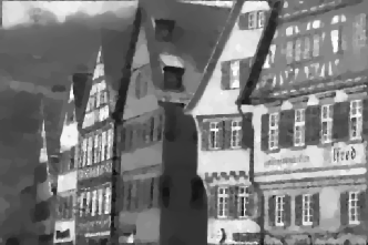
Figure 7. Denoising results for $20\%$ Gaussian noise. First row: $\text{L}^{2}$ - and Bregman oracle. Middle row: SA-TV with window size $11$ and $19$. Last row: SMREs w.r.t. $\mathcal{S}_{0}$ and $S_{2}$ (with $\alpha=0.9$).

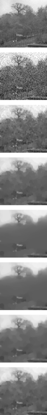
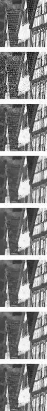
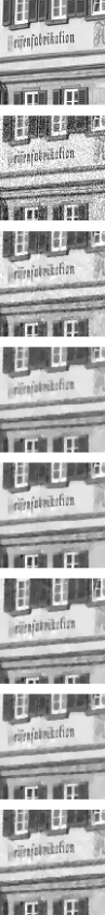
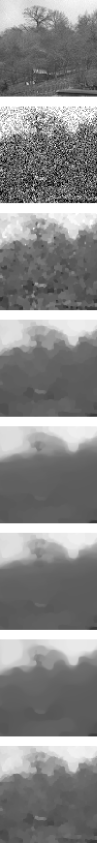
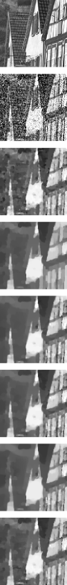
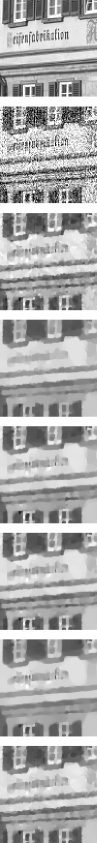
Figure 8. Reconstruction details for $10\%$ (left frame) and $20\%$ (right frame) Gaussian noise. From top to bottom: True signal, data, $\text{L}^{2}$- and Bregman oracle, SA-TV with window size $11$ and $19$, SMRE w.r.t. $\mathcal{S}_{0}$ and $\mathcal{S}_{2}$ and $\alpha=0.9$

We compare our estimators to the global estimators $\hat{u}(\lambda)$ ($\lambda>0$) as defined in (2). We choose $\lambda=\lambda_{2}$ and $\lambda=\lambda_{\text{B}}$ such that the mean squared distance and the mean symmetric Bregman distance to the true signal $u^{0}$ is minimized, respectively. To be more precise, we set

$$\lambda_{2}=\mathbf{E}\left(\operatorname*{\textnormal{argmin}}_{\lambda>0}\left\|u^{0}-\hat{u}(\lambda)\right\|^{2}\right)\;\text{ and }\;\lambda_{\text{B}}=\mathbf{E}\left(\operatorname*{\textnormal{argmin}}_{\lambda>0}D_{J}^{\text{sym}}(u^{0},\hat{u}(\lambda))\right),$$ (29)

where the symmetric Bregman distance for $J$ as in (3) formally reads as

$$D^{\text{sym}}_{J}(u,v) =\sum_{(i,j)\in G}\left(\frac{\nabla u_{ij}}{\left|\nabla u_{ij}\right|}-\frac{\nabla v_{ij}}{\left|\nabla v_{ij}\right|}\right)\cdot\left(\nabla u_{ij}-\nabla v_{ij}\right)$$

$$=\sum_{(i,j)\in G}(\left|\nabla u_{ij}\right|+\left|\nabla v_{ij}\right|)\left(1-\frac{\nabla u_{ij}\cdot\nabla v_{ij}}{\left|\nabla u_{ij}\right|\left|\nabla v_{ij}\right|}\right).$$

This means that $D^{\text{sym}}_{J}(u,v)$ is small if for sufficiently many pixels $(i,j)\in G$ either both $u$ and $v$ are constant in a neighborhood of $(i,j)$ or the level lines of $u$ and $v$ at $(i,j)$ are locally parallel. In practice, we rather use

$$J(u)=\sum_{(i,j)\in G}\sqrt{|\nabla u_{ij}|_{2}^{2}+\beta^{2}}$$

instead of $J$ in (3) for some small constant $\beta\approx 10^{-8}$. Then the above formulae are slightly more complicated. Since the parameters $\lambda_{2}$ and $\lambda_{\text{B}}$ are not accessible in practice as $u^{0}$ is unknown, we refer to $\hat{u}(\lambda_{2})$ and $\hat{u}(\lambda_{\text{B}})$ as $\text{L}^{2}$- and Bregman-oracle, respectively. Simulations lead values $\lambda_{2}=0.026,0.0789$ and $\lambda_{\text{B}}=0.0607,0.1767$ for $\sigma=0.1,0.2$, respectively.

In addition, we compare our approach to the spatially adaptive TV (SA-TV) method as introduced in [11]. The SA-TV algorithm approximates solutions of (6) for the case where $\mathcal{S}$ constitutes the set of all translates of a fixed window $S\subset G$ (cf. also [1]) by computing a solution of (5) with a suitable spatially dependent regularization parameter $\lambda$. Starting from a (constant) initial parameter $\lambda\equiv\lambda_{0}$ the SA-TV algorithm iteratively adjusts $\lambda$ by increasing it in regions that were poorly reconstructed in the previous step. For our numerical comparisons, we used the SA-TV-Algorithm considering square windows with side lengths $11$ (as suggested in [11]) and $19$. All parameters involved in the algorithm were chosen as suggested in [11]. In particular we set $\lambda_{0}=0.5$ and choose an upper bound for $\lambda$ of $L=1000$ in all our simulations. As a stopping condition, we used the discrepancy principle which ended the reconstruction process after exactly four iteration steps in all of our experiments.

The reconstructions are displayed in Figure 6 ($\sigma=0.1$) and Figure 7 ($\sigma=0.2$). By visual inspection, we find that the oracles are globally under- ($\text{L}^{2}$) and over-regularized (Bregman), respectively. While the scalar parameter $\lambda$ was chosen optimally w.r.t. the different distance measures, it still cannot cope with the spatially varying smoothness of the true object $u^{0}$.

In contrast, SMRE and SA-TV reconstructions exhibit the desired locally adaptive behaviour. Still, the SMRE as formulated in this paper has the advantage that multiple scales are taken into account at once, while SA-TV only adapts the parameter on a single given scale. As a result, SA-TV reconstructions are of varying quality for finer and coarser features of the object, while the SMRE is capable of reconstructing such features equally well. This becomes particularly obvious when zooming into the reconstructions (cf. Figure 8).

5.2. Deconvolution & Inpainting

We next investigate the performance of our approach if the operator $K$ in (1) is non-trivial. To be exact, we consider inpainting and deconvolution problems. For the first we consider an inpainting domain that occludes $15\%$ of the image with noise level $\sigma=0.1$ (upper left panel in Figure 9) and for the latter a Gaussian convolution kernel with variance $2$ and noise level $\sigma=0.02$ (lower left panel in Figure 9).

For all experiments we use the dyadic system $\mathcal{S}_{2}$ and $\alpha=0.9$. Note that in both cases we have $K=K^{*}$ and $\left\|K\right\|=1$; we therefore set $\zeta=1.01$ in (15). The results are depicted in the upper right and lower right images of Figure 9, respectively.

Again, the results indicate that a reasonable trade-off between data fit and smoothing is found by the proposed a priori parameter choice rule and that the amount of smoothing is adapted according to the image features.

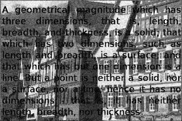
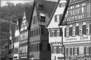
Figure 9. Inpainting (top): data $Y$ with $\sigma=0.1$ (left) and SMRE (right). Deconvolution (bottom): data $Y$ with $\sigma=0.02$ (left) and SMRE (right).

5.3. Examples from Fluorescence Microscopy

We finally study the performance of our approach in a practical application, namely fluorescence microscopy. To be more precise, we consider deconvolution problems for standard confocal microscopy and STED (STimulated Emission Depletion) microscopy. Both examples have in common, that the recorded data is a realization of independent Poisson variables where the intensity at each pixel is determined by a blurred version of true signal. In other words, Model (8) applies. In both cases the blurring can be modelled (in first order) as a convolution with a Gaussian kernel where the width of the kernel for confocal microscopes is $3-4$ times larger than it is for STED. As standard references we refer to [32] (confocal microscopy) and to [25, 24] (STED).

In both cases, we will use sample images of PtK2 cells taken from the kidney of potorous tridactylus, where beforehand the protein $\beta$-tubulin was tagged with a fluorescent marker. What becomes visible is the microtubule part of the cytosceleton of the cells. The left panels in Figures 10 and 12 show the confocal and STED recordings, respectively. Both sample images show an area of $18\times 18$$\upmu$m² at a resolution of $798\times 798$ pixels. As a regularization functional we use in both cases a combination of the total variation semi-norm and the $\text{L}^{2}$-norm as in (4) with $\gamma=1$.

5.3.1. Confocal microscopy

Figure 10 depicts a confocal recording of a PtK2 cell (left) and the solution of (21) computed by Algorithm 2 (right). We have used the subset of $\mathcal{S}_{0}$ with maximal side length of $20$ pixel and the scale weights $c_{S}$ are chosen as in Proposition 2.3 with $\alpha=0.9$. For the convolution kernel we assume a full width at half maximum of $230$nm which corresponds to a standard deviation of 4.3422 pixels. Due to this relatively large kernel, the impact of the deconvolution is clearly visible.

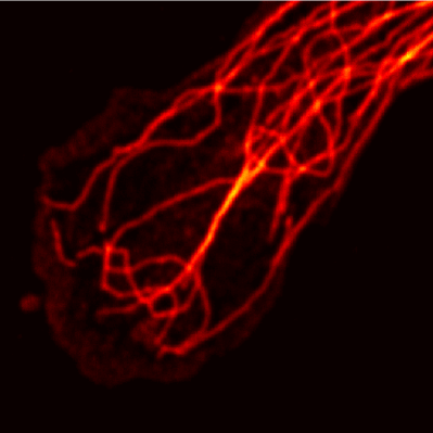
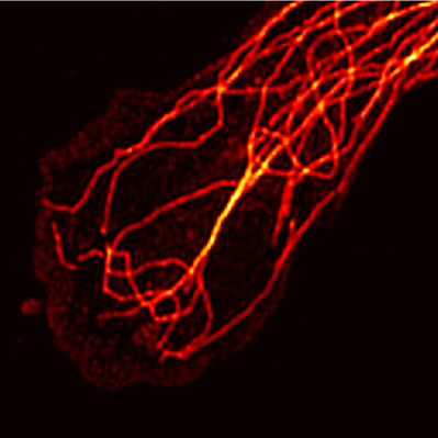
Figure 10. Confocal deconvolution: data $Y$ (left) and SMRE (right).

This becomes remarkably apparent when one takes a closer look: In Figure 11 a zoomed-in area of the data (left) and the SMRE (right) is depicted. Clearly, the reconstruction reveals details that are not visible (or at least not apparent) in the data. In particular, the individual microtubule-filaments are separated properly.

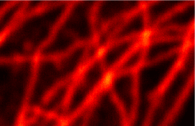
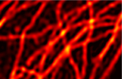
Figure 11. Confocal deconvolution (closer look): data $Y$ (left) and SMRE (right).

We finally remark, that we proposed a different multi-scale deconvolution method for confocal microscopy in [19]. In contrast to this work, we there used a different MR-statistic than $T$ in (7) and we used the standardization $(Y-\beta)/\sqrt{\beta}$ in order to transform the Poisson data $Y$ to normality. The performance of the two approaches for confocal recording is comparable since the image intensity (=photon count rate) is relatively high throughout the data and hence standardization yields a fair approximation to normality. However, for low-count Poisson data, as we will investigate in the following section, our new approach is clearly preferable, mostly due to the fact that Anscombe’s transform also works well for small intensities (cf. [5]).

5.3.2. STED microscopy

The left panel of Figure 12 depicts a STED recording of a PtK2 cell. For the convolution kernel a full width at half maximum of $70$nm is assumed, which corresponds to a standard deviation of approximately $1.1327$ pixels. The right image of Figure 12 depicts an approximate solution of (21) that was computed by Algorithm 2. Again we use the system $\mathcal{S}$ of all squares in $\mathcal{S}_{0}$ up to a maximal side length of $20$ pixels and the thresholds $c_{S}$ are chosen according to Proposition (2.3) with $\alpha=0.9$. Due to the relatively small convolution kernel, the impact of the deconvolution is less striking as e.g. for the confocal recording in Paragraph 5.3.1.

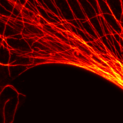
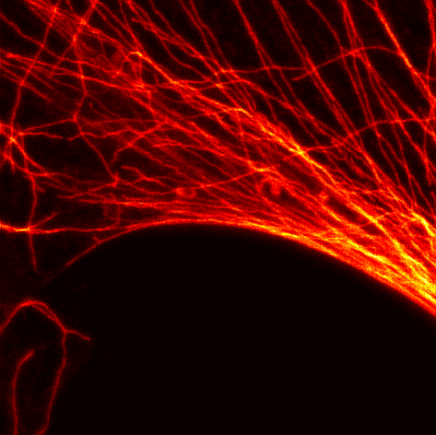
Figure 12. STED deconvolution: data $Y$ (left) and SMRE (right).

When zooming into the image, the effect becomes more obvious: The left and middle panel in Figure 13 depicts a detailed view on the STED data and the SMRE from Figure 12. The right panel in Figure 13 shows the global reconstruction $\hat{u}_{\text{g}}$, i.e. we computed a solution of (21) w.r.t. to the trivial system $\mathcal{S}=\left\{G\right\}$ and the parameter $c_{G}$ as in Proposition 2.3 with $\alpha=0.9$. The global reconstruction exhibits typical concentration phenomena (especially in the upper half of the image) that are due to the ill-posedness of the deconvolution. These artefacts are less prominent for the SMRE solution.

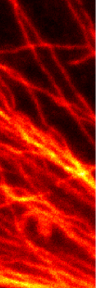
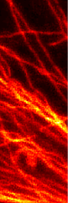
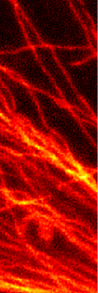
Figure 13. STED deconvolution (detail): data $Y$ (left), SMRE (middle) global reconstruction (right)

At the same time, some parts of $\hat{u}_{\text{g}}$ are oversmoothed. In Figure 14 the union of the sets $S\in\mathcal{S}_{0}$ where

$$c_{S}\sum_{(i,j)\in S}\left|2\sqrt{Y_{ij}+3/8}-2\sqrt{K\hat{u}_{\text{g}}}\right|>1$$

are highlighted, where we restrict our consideration to the squares with a sidelength of $7$ pixel. A closer view on the highlighted subset confirms the oversmoothing (lower zoom-box). Again we note that at the same time the global image reconstruction has artefacts due to the ill-posedness of the deconvolution (upper zoom-box). These can only be avoided by invoking stronger regularization. A comparison with the corresponding details of the SMRE (right) shows that our locally adaptive approach lacks this undesirable behaviour.

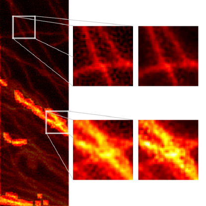
Figure 14. Oversmoothed regions in the global estimator $\hat{u}_{\text{g}}$ identified on the scales $\left|S\right|=7$. Zoomed-in regions show over- (lower zoom-box) and underregularized (upper zoom-box) parts in the image that do not occur in the SMRE reconstruction (right boxes).

6. Conclusion

In this paper we show how statistical multiresolution estimators, that is solutions of (6), can be employed for image reconstruction. We stress that our method, combined with a new automatic selection rule, locally adapts the amount of regularization according to the multi-scale nature of the image features. For the solution of the optimization problem (6) we suggest an inexact alternating direction method of multipliers combined with Dykstra’s projection algorithm. We show how this estimation paradigm can be extended to the Poisson model which opens up a vast field of applications, such as Poisson nanoscale fluorescence microscopy. Aside to this application, the performance of our method is illustrated for standard problems in imaging such as denoising and inpainting.

Acknowledgments

K.F. and A.M. are supported by the DFG–SNF Research Group FOR916 Statistical Regularization and Qualitative Constraints (Z-Project). P.M is supported by the BMBF project $03$MUPAH$6$ INVERS. A.M. and P.M. are supported by the SFB755 Nanoscale Photonic Imaging and the SFB803 Functionality Controlled by Organization in and between Membranes. The authors are indebted to S. Hell, A. Egner and A. Schoenle (Department of NanoBiophotonics, Max Planck Institute for Biophysical Chemistry, Göttingen and Laser Laboratorium Göttingen) for providing the microscopy data and for fruitful discussions.

References

- [1] A. Almansa, C. Ballester, V. Caselles, and G. Haro. A TV based restoration model with local constraints. J. Sci. Comput., 34(3):209–236, 2008.
- [2] M. Bertalmio, V. Caselles, B. Rougé, and A. Solé. TV based image restoration with local constraints. J. Sci. Comput., 19(1-3):95–122, 2003.
- [3] M. Bertero and P. Boccacci. Image restoration methods for the large binocular telescope (lbt). Astron. Astrophys. Suppl. Ser., 147(2):323–333, 2000.
- [4] J. P. Boyle and R. L. Dykstra. A method for finding projections onto the intersection of convex sets in Hilbert spaces. In Advances in order restricted statistical inference (Iowa City, Iowa, 1985), volume 37 of LNS, pages 28–47. Springer, Berlin, 1986.
- [5] L. Brown, T. Cai, R. Zhang, L. Zhao, and H. Zhou. The root-unroot algorithm for density estimation as implemented via wavelet block thresholding. Probab. Theory Related Fields, 146(3-4):401–433, 2010.
- [6] D. Butnariu, Y. Censor, and S. Reich, editors. Inherently parallel algorithms in feasibility and optimization and their applications, volume 8 of Studies in Computational Mathematics. North-Holland Publishing Co., Amsterdam, 2001. Papers from the Research Workshop held jointly at the University of Haifa and at the Technion–Israel Institute of Technology, Haifa, March 13–16, 2000.
- [7] A. Chambolle. An algorithm for total variation minimization and applications. J. Math. Imaging Vision, 20(1–2):89–97, 2004.
- [8] A. Chambolle and P.-L. Lions. Image recovery via total variation minimization and related problmes. Numer. Math., 76(2):167–188, 1997.
- [9] A. Chambolle and T. Pock. A first-order primal-dual algorithm for convex problems with applications to imaging. J. Math. Imaging Vision, 40:120–145, 2011.
- [10] D. C. Dobson and C. R. Vogel. Convergence of an iterative method for total variation denoising. SIAM J. Numer. Anal., 34(5):1779–1791, 1997.
- [11] Y. Dong, M. Hintermüller, and M. M. Rincon-Camacho. Automated regularization parameter selection in multi-scale total variation models for image restoration. J. Math. Imaging Vision, 40(1):82–104, 2011.
- [12] I. Ekeland and R. Temam. Convex analysis and variational problems, volume 1 of Studies in Mathematics and its Applications. North-Holland Publishing Co., Amsterdam-Oxford, 1976.
- [13] H. C. Elman and G. H. Golub. Inexact and preconditioned Uzawa algorithms for saddle point problems. SIAM J. Numer. Anal., 31(6):1645–1661, 1994.
- [14] E. Esser, X. Zhang, and T. F. Chan. A general framework for a class of first order primal-dual algorithms for convex optimization in imaging science. SIAM J. Imaging Sci., 3(4):1015–1046, 2010.
- [15] G. Facciolo, A. Almansa, J.-F. Aujol, and V. Caselles. Irregular to regular sampling, denoising, and deconvolution. Multiscale Model. Simul., 7(4):1574–1608, 2009.
- [16] M. Fortin and R. Glowinski. Augmented Lagrangian methods, volume 15 of Studies in Mathematics and its Applications. North-Holland Publishing Co., Amsterdam, 1983. Applications to the numerical solution of boundary value problems.
- [17] K. Frick and P. Marnitz. A statistical multiresolution strategy for image reconstruction. In A. Bruckstein, B. ter Haar Romeny, A. Bronstein, and M. Bronstein, editors, Scale Space and Variational Methods in Computer Vision, volume 6667 of Lecture Notes in Computer Science, pages 74–85. Springer Berlin / Heidelberg, 2012.
- [18] K. Frick, P. Marnitz, and A. Munk. Shape constrained regularisation by statistical multiresolution for inverse problems: Asymptotic analysis. Inverse Problems, 2012. To appear.
- [19] K. Frick, P. Marnitz, and A. Munk. Statistical multiresolution Dantzig estimation in imaging: Fundamental concepts and algorithmic framework. Electron. J. Stat., 6:231–268, 2012.
- [20] K. Frick and O. Scherzer. Convex inverse scale spaces. In F. Sgallari, A. Murli, and N. Paragios, editors, SSVM, volume 4485 of LNCS, pages 313–325. Springer, 2007.
- [21] G. Gilboa, N. Sochen, and Y. Zeevi. Variational denoising of partly textured images by spatially varying constraints. Image Processing, IEEE Transactions on, 15(8):2281–2289, 2006.
- [22] M. Grasmair. Locally adaptive total variation regularization. In X.-C. Tai, K. Mørken, M. Lysaker, and K.-A. Lie, editors, Scale Space and Variational Methods in Computer Vision, volume 5567 of Lecture Notes in Computer Science, pages 331–342. Springer Berlin / Heidelberg, 2009.
- [23] D. M. Hawkins and R. Wixley. A note on the transformation of chi-squared variables to normality. Amer.Statist., 40(4):296–298, 1986.
- [24] S. W. Hell. Far-Field Optical Nanoscopy. Science, 316(5828):1153–1158, 2007.
- [25] S. W. Hell and J. Wichmann. Breaking the diffraction resolution limit by stimulated emission: stimulated-emission-depletion fluorescence microscopy. Opt. Lett., 19(11):780–782, 1994.
- [26] M. Hintermüller and K. Kunisch. Total bounded variation regularization as a bilaterally constrained optimization problem. SIAM J. Appl. Math., 64(4):1311–1333, 2004.
- [27] T. Hotz, P. Marnitz, R. Stichtenoth, L. Davies, Z. Kabluchko, and A. Munk. Locally adaptive image denoising by a statistical multiresolution criterion. Comput. Stat. Data An., 56(3):543 – 558, 2012.
- [28] Z. Kabluchko. Extremes of the standardized Gaussian noise. Stochastic Process. Appl., 121(3):515–533, 2011.
- [29] Z. Kabluchko and A. Munk. Shao’s theorem on the maximum of standardized random walk increments for multidimensional arrays. ESAIM Probab. Stat., 13:409–416, 2009.
- [30] A. Munk, N. Bissantz, T. Wagner, and G. Freitag. On difference-based variance estimation in nonparametric regression when the covariate is high dimensional. J. R. Stat. Soc. Ser. B Stat. Methodol., 67(1):19–41, 2005.
- [31] S. Osher, M. Burger, D. Goldfarb, J. Xu, and W. Yin. An iterative regularization method for total variation-based image restoration. Multiscale Model. Simul., 4(2):460–489 (electronic), 2005.
- [32] J. B. Pawley. Handbook of Biological Confocal Microscopy. Springer, 2006.
- [33] L. I. Rudin, S. Osher, and E. Fatemi. Nonlinear total variation based noise removal algorithms. Phys. D, 60:259–268, 1992.
- [34] E. Tadmor, S. Nezzar, and L. Vese. A multiscale image representation using hierarchical decompositions. Multiscale Model. Simul., 2(4):554–579 (electronic), 2004.
- [35] Y. Vardi, L. A. Shepp, and L. Kaufman. A statistical model for positron emission tomography. J. Amer. Statist. Assoc., 80(389):8–37, 1985. With discussion.
- [36] X. Zhang, M. Burger, X. Bresson, and S. Osher. Bregmanized nonlocal regularization for deconvolution and sparse reconstruction. SIAM J. Imaging Sci., 3(3):253–276, 2010.
- [37] W. P. Ziemer. Weakly differentiable functions. Springer Verlag, New York, 1989.