Coarsening scenarios in unstable crystal growth

Abstract

Crystal surfaces may undergo thermodynamical as well kinetic, out-of-equilibrium instabilities. We consider the case of mound and pyramid formation, a common phenomenon in crystal growth and a long-standing problem in the field of pattern formation and coarsening dynamics. We are finally able to attack the problem analitycally and get rigorous results. Three dynamical scenarios are possible: perpetual coarsening, interrupted coarsening, and no coarsening. In the perpetual coarsening scenario, mound size increases in time as $L\sim t^{n}$, where the coasening exponent is $n=1/3$ when faceting occurs, otherwise $n=1/4$.

Introduction.—The still ongoing large interest towards instabilities in crystal growth RMP_Chaouqi can be motivated by its lying in between the practical problem of controlling the growth processes and the fundamental domain of out-of-equilibrium transitions and pattern formation. Even if some phenomena may be studied in one spatial dimension 1d , most interesting physics of surface growth occurs in two spatial dimensions, where rigorous approaches are rare and numerical simulations are more problematic and much more time consuming.

The unstable growth of a crystal surface has some similarities with phase ordering processes, for which the analysis of Bray Bray is the most comprehensive and successful theory (see also Refs. Cugliandolo ; 2d for more recent results). However, in two dimensions growth has peculiar features review_Paolo , because the natural order parameter, the surface slope $\mathbf{m}$, obeys a special constraint $(\nabla\times\mathbf{m}=0$), so that resulting domain walls must be straight, which is not the case with other phase ordering phenomena. As a consequence of that, rigorous analytical approaches to crystal growth instabilities are very rare. A paper by Watson and Norris Watson , based on the principle of maximal dissipation and a couple of papers Kohn ; BoLi providing exact inequalities for the coarsening exponent are some of the few examples. Other interesting, albeit heuristic, approaches had contributed significantly to our understanding of coarsening Rost_Krug ; Golubovic1997 ; tang .

At the general level, we think that mound formation in two dimensional crystal growth, in spite of being quite an old problem Villain , still lacks a systematic and rigorous approach. In this manuscript we propose to fill this gap. We start by briefly reminding the basic phenomenology of unstable crystal growth which is of interest to us and presenting a well established continuum description of the growing surface. Then the central part of the paper follows: the application of the phase diffusion concept that allows to face at once a large class of models and symmetries. In this approach, the pattern instability is signaled by a negative phase diffusion coefficient, which implies coarsening, i.e. an increase of the size $L$ of the pattern. In the case of perpetual coarsening, the dependence of the diffusion coefficient on $\lambda$ allows to determine the growth law, $L(t)$. Our work gives the first rigorous, general framework to study unstable crystal growth and we provide important results concerning coarsening scenarios and coarsening exponents.

Phenomenology and model.—Here we focus on deposition processes on a high symmetry substrate, where atoms or molecules arrive ballistically and thermally diffuse until they are incorporated into the crystal RMP_Chaouqi . A key process, which is the possible cause of the instability, is the attachment to steps: if adatoms stick to ascending steps more efficiently than to descending steps, an uphill current forms and the growing surface destabilizes, forming a mound structure.

Experimental results are available for many systems, specially metals, and different dynamical scenarios have appeared. Cu(100) Cu100 and Rh(111) Rh111 are examples of a coarsening process which occurs during the whole experimental time scale. Instead, Pt(111) Pt111 is a prototype for coarsening which immediately stops or does not even start, while the height of mounds goes on increasing. In some cases, slopes of mound tend to constant values, corresponding to faceting. In other cases, observed slopes increase as well. Finally, the symmetry of the pattern is related to the unstable orientation: (100) surfaces produce a $4$-fold pattern, while (111) surfaces produce a $3$-fold pattern 111 . The quantitative determination of the coarsening exponent, when appropriate, is made extremely difficult by the short experimental time scale over which $L(t)$ is measured and by the relatively smallness of the coarsening exponent, $n\lesssim\frac{1}{3}$.

Theoretical work has accompanied experiments with Kinetic Monte Carlo simulations KMC and with continuum approaches review_Paolo , where the dynamics of the local height of the surface, $h(\mathbf{x},t)$, is governed by a partial differential equation. Much effort has been devoted to give robustness to the equations, while the equations themselves have been mainly studied numerically. Here below we propose a more systematic and rigorous approach in the continuum limit, starting from the well established class of equations:

$$\frac{\partial h(\mathbf{x},t)}{\partial t}=-\mathbf{\nabla}\cdot{[\mathbf{j}(\nabla h)+\mathbf{\nabla}(\nabla^{2}h)]}\equiv-\mathbf{\nabla}\cdot{\mathbf{J}_{tot}},$$ (1)

whose conservative form signals that, at the experimental conditions usually set for these deposition processes, overhangs and evaporation are negligible. The total current, $\mathbf{J}_{tot}$, is composed of two terms: the nonequilibrium, slope dependent current, $\mathbf{j}(\nabla h)$, describes the effects of the Ehrlich-Schwoebel barrier, which hinders adatoms to stick to the lower step, with $\mathbf{j}\simeq\nabla h$ for $|\nabla h|\ll 1$ Villain ; the second term, $\mathbf{\nabla}(\nabla^{2}h)$, is the Mullins term, describing termal detachment of adatoms from steps and nonequilibrium effects Rodi . In Eq. (1), the white noise due to the flux can be omitted Bray . We would like to highlight that we do not give explicit form to the slope dependent $\mathbf{j}$: our analytical approach embraces any current $\mathbf{j}$. We can even add that Eq. (1) is also relevant for thermodynamically unstable surfaces spinodal .

The method.— Equation (1) admits the trivial solution $h\equiv 0$, corresponding to the flat profile. Setting $h=\delta~{}\hbox{exp}(\omega t+i\mathbf{k}\cdot\mathbf{x})$ and linearizing in $\delta$ yields $\omega(k)=k^{2}-k^{4}$, $k=|\mathbf{k}|$, showing linear exponential growth, until the nonlinearity can no longer be neglected.

The amplitude growth of mounds is thus fast, while wavelength rearrangement (if any) is slow and follows a diffusion process, as seen below. At short time scale the structure assumes a periodic pattern defined by two basis wave vectors $\mathbf{q}_{1}$,$\mathbf{q}_{2}$, or, similarly, by the two phases $\varphi_{i}=\mathbf{q}_{i}\cdot\mathbf{x}$. The slow evolution of the phase makes it legitimate to introduce, besides the fast variable $\mathbf{x}$, a slow dependence on time and space, $T$ and $\mathbf{X}$, so that the local wave vector $\mathbf{q}=\mathbf{q}(T,\mathbf{X})$. Owing to the diffusion character of the phase, we expect $T=\varepsilon^{2}t$ and $\mathbf{X}=\varepsilon\mathbf{x}$, where $\varepsilon$ is a small parameter measuring the long wavelength modulation (small gradient) of the phase. It is convenient to introduce slow phases, related to the fast one by $\psi_{i}=\varepsilon\varphi_{i}$, so that $\mathbf{q}_{i}=\nabla_{\mathbf{x}}\varphi_{i}=\nabla_{\mathbf{X}}\psi_{i}$. In a multiscale spirit, from these definition together with $h=h_{0}+\varepsilon h_{1}+\dots$, the following expansions for the operators hold:

$$\partial_{t} = \varepsilon\left((\partial_{T}\psi_{1})\partial_{\varphi_{1}}+(\partial_{T}\psi_{2})\partial_{\varphi_{2}}\right)$$ (2)

$$\nabla = \nabla_{0}+\varepsilon\nabla_{\mathbf{X}},$$ (3)

with $\nabla_{0}=\mathbf{q}_{1}\partial_{\varphi_{1}}+\mathbf{q}_{2}\partial_{\varphi_{2}}$ and $\nabla_{\mathbf{X}}=(\partial_{X},\partial_{Y})$. Finally, the current $\mathbf{j}$ reads:

$$\mathbf{j}(\nabla h)=\mathbf{j}(\nabla_{0}\tilde{h}_{0})+\varepsilon\mathcal{J}(\nabla_{0}\tilde{h}_{1}+\nabla_{\mathbf{X}}\tilde{h}_{0}),$$ (4)

where $\mathcal{J}$ is the Jacobian matrix. Reporting the above expansions into Eq. (1) we obtain successively higher order contributions in powers of $\varepsilon$. To order $\varepsilon^{0}$ we gain

$$0=\nabla_{0}\cdot{[\mathbf{j}(\nabla_{0}\tilde{h}_{0})+\nabla_{0}(\nabla_{0}^{2}\tilde{h}_{0})]}=\nabla_{0}\cdot{(\mathbf{J}_{0})_{tot}}\equiv\mathcal{N}[\tilde{h}_{0}],$$ (5)

which is a nonlinear equation satisfied by the steady-state profile $\tilde{h}_{0}$. Since we are interested in growth on high symmetry substrates, the stronger condition $(\mathbf{J}_{0})_{tot}=0$ is fulfilled. Then, to first order we obtain:

$$\mathcal{L}[\tilde{h}_{1}]=g(\tilde{h}_{0},\psi_{1},\psi_{2}),$$ (6)

where

$$\mathcal{L}[\tilde{h}_{1}]\equiv-\nabla_{0}\cdot{[\mathcal{J}(\nabla_{0}\tilde{h}_{1})+\nabla_{0}(\nabla_{0}^{2}\tilde{h}_{1})]}$$ (7)

is the Fréchet derivative of $\mathcal{N}$, and

$$\begin{split}g&\equiv(\partial_{T}\psi_{1})\partial_{\varphi_{1}}\tilde{h}_{0}+(\partial_{T}\psi_{2})\partial_{\varphi_{2}}\tilde{h}_{0}+\nabla_{0}\cdot[\mathcal{J}(\nabla_{\mathbf{X}}\tilde{h}_{0})\\ &+\nabla_{\mathbf{X}}(\nabla_{0}^{2}\tilde{h}_{0})+\nabla_{0}(\nabla_{1}^{2}\tilde{h}_{0})].\end{split}$$ (8)

In order to avoid secular terms, we use the Fredholm’s alternative theorem zwillinger , according to which Eq. (6) has solutions if and only if $\langle v,g\rangle=0$ scalarproduct , where ${\cal L}^{\dagger}[v]=0$.

While the derivation of the phase equation can be achieved for any nonlinear equation, we focus here on Eqs. (1) such that $\mathcal{L}$ is a self-adjoint operator, $\mathcal{L}^{\dagger}=\mathcal{L}$. This condition is equivalent to saying that the Jacobian ${\cal J}$ is symmetric, which, in fact, is not a restriction: all surface currents $\mathbf{j}$ discussed in the literature provide a symmetric ${\cal J}$. Thanks to the translational invariance of $\mathcal{N}$ with respect to the space variable, we easily obtain non trivial solutions of the form $v_{i}=\partial_{\varphi_{i}}h_{0}$, $i=1,2$ (Goldstone mode). This leads us to two diffusion equations ($i=1,2$):

$$\partial_{T}\psi_{i}=\frac{\partial\psi_{\alpha}}{\partial X_{\beta}\partial X_{\gamma}}\tilde{D}_{\beta\gamma}^{i\alpha},~{}~{}~{}~{}~{}\alpha,\beta,\gamma=1,2$$ (9)

where the diffusion coefficients have the following expressions:

$$\tilde{D}_{\beta\gamma}^{1\alpha}=\left[\frac{\langle h_{1},c^{\alpha}_{\beta\gamma}\rangle\langle h_{2},h_{2}\rangle-\langle h_{2},c^{\alpha}_{\beta\gamma}\rangle\langle h_{1},h_{2}\rangle}{\langle h_{1},h_{1}\rangle\langle h_{2},h_{2}\rangle-{\langle h_{1},h_{2}\rangle}^{2}}\right]$$ (10)

and $\tilde{D}_{\beta\gamma}^{2\alpha}~{}\begin{subarray}{c}{1\leftrightarrow 2}\\ \displaystyle=\end{subarray}~{}\tilde{D}_{\beta\gamma}^{1\alpha}$. Here above we have introduced the more compact notation $h_{j}=\partial_{\varphi_{j}}\tilde{h}_{0}=\partial_{j}\tilde{h}_{0}$, and

$$\begin{split}-c^{\alpha}_{\beta\gamma}&=q_{\delta\nu}\partial_{\varphi_{\delta}}\left[\mathcal{J}_{\nu\gamma}\frac{\partial h_{0}}{\partial q_{\alpha\beta}}\right]+2q_{j\gamma}q_{l\beta}\partial_{\alpha}\partial_{l}\partial_{j}h_{0}\\ &+3\nabla_{0}^{2}q_{\nu\beta}\partial_{\nu}\frac{\partial h_{0}}{\partial q_{\alpha\gamma}}+\delta_{\beta\gamma}\nabla_{0}^{2}\partial_{\alpha}h_{0},\end{split}$$ (11)

where the use of the zeroth order relation $\mathbf{j}(\nabla_{0}\tilde{h}_{0})=-\nabla_{0}(\nabla_{0}^{2}\tilde{h}_{0})$ has allowed to replace the current with derivatives of the steady profile.

We conclude this part stressing that our $\epsilon-$expansion might continue at higher order, leading to nonlinear terms in Eqs. (9). We refer the reader to the discussion in 1d , Sect. VIĊ.

Pattern symmetries and phase diffusion equations—For definiteness we focus in the following on square (4-fold) and hexagonal (6-fold) patterns. In the square case, we set $\mathbf{q}_{1}=q(1,0)$ and $\mathbf{q}_{2}=q(0,1)$ and exploiting parity and $4$-fold symmetry for $\tilde{h}_{0}$, physical properties are equivalent upon the changes $\varphi_{1}\leftrightarrow\varphi_{2}$. In the hexagonal case, we have $\mathbf{q}_{1}=q(1/2,\sqrt{3}/2)$ and $\mathbf{q}_{2}=q(1/2,-\sqrt{3}/2)$ and parity and $6$-fold symmetry imply invariance under the changes $(\varphi_{1}\leftrightarrow\varphi_{2})$ and $(\varphi_{1}\rightarrow-\varphi_{2}$, $\varphi_{2}\rightarrow\varphi_{1}+\varphi_{2})$. The interesting result is that, for both symmetries, Eqs. (9) assume a much simpler form diff.coeff :

$$\partial_{T}\psi_{1}=(\psi_{1})_{11}D_{11}+(\psi_{1})_{22}D_{22}+(\psi_{2})_{12}D_{12}$$ (12a)

$$\partial_{T}\psi_{2}=(\psi_{1})_{12}D_{12}+(\psi_{2})_{11}D_{22}+(\psi_{2})_{22}D_{11},$$ (12b)

with only three non vanishing diffusion coefficients. The hexagonal pattern enjoys an additional property:

$$D_{11}-D_{22}-D_{12}=0,$$ (13)

leaving us with only two independent diffusion coefficients.

Phase instability means wavelength rearrangement, leading to coarsening. To investigate stability of the pattern we set $\psi_{1,2}(\mathbf{X},T)=\psi_{1,2}^{(0)}\exp{(\Omega T)}\exp{(i\mathbf{K}\cdot\mathbf{X})}$, where instability is signaled by at least one positive eigenvalue $\Omega_{1,2}(\mathbf{K})$. In the hexagonal case we straightforwardly find from Eqs. (12) that:

$$\Omega_{1}=-D_{22}K^{2}\,,~{}~{}\Omega_{2}=-D_{11}K^{2}.$$ (14)

Since $D_{ij}$ are expressed in terms of integrals involving the steady periodic pattern $h_{0}$ (see Eq.(10)), stability can be linked to the property of steady-state solutions only. It is a simple matter to show that $D_{22}$ is positive, thus $\Omega_{1}<0$. The analysis of $D_{11}$ is much more involved. After several manipulations we find:

$$D_{11}=\frac{4q^{7/4}}{\langle h_{1}^{2}\rangle}\partial_{q}(q^{5/4}\langle h_{12}^{2}\rangle)~{}\equiv~{}f(q)\mathcal{A}^{\prime}(q).$$ (15)

The sign of $D_{11}$ (and thus of $\Omega_{2}$) is given by the sign of the slope of the function $\mathcal{A}=(q^{5/4}\langle h_{12}^{2}\rangle)$ with respect to $q$. In the 1D models studied in 1d this function was found to be the amplitude of the steady state solutions. The present study reveals a new class of dynamics where the relevant quantity is $\mathcal{A}(q)$, having a more abstract meaning than just the amplitude itself. At present a simple physical interpretation of this function is missing.

For square symmetry, the spectrum is anisotropic, depending on the angle $\theta$ between $\mathbf{K}$ and the $X$ axis. However, symmetry imposes that the growth rate may be maximal along two directions: (i) $\theta=0$, for which $\Omega_{1}^{0}(K)=-D_{22}K^{2}$ and $\Omega_{2}^{0}(K)=-D_{11}K^{2}$, and (ii) $\theta=\pi/4$, for which $\Omega_{1}^{\pi/4}(K)=-(D_{11}+D_{22}-D_{12})K^{2}/2$ and $\Omega_{2}^{\pi/4}(K)=-(D_{11}+D_{22}+D_{12})K^{2}/2$. Again, the stability is dictated by the sign of diffusion coefficients: we find that the eigenvalues $\Omega_{1}^{0,\pi/4}$ are negative, while the eigenvalues $\Omega_{2}^{0,\pi/4}$ have no fixed sign:

$$D_{11}=\frac{1}{\langle h_{1}^{2}\rangle}[\partial_{q}(q^{3}\langle h_{11}^{2}\rangle)+q^{3}\partial_{q}\langle h_{12}^{2}\rangle+q^{2}\langle h_{12}^{2}\rangle],$$ (16a)

$$\begin{split}D_{11}&+D_{22}+D_{12}=\frac{4}{\langle h_{1}^{2}\rangle}\left[\frac{1}{2}q^{3}\partial_{q}\langle h_{11}^{2}\rangle+q^{2}\langle h_{11}^{2}\rangle\right.\\ &+\left.\frac{1}{2}q^{3}\partial_{q}\langle h_{12}^{2}\rangle+2q^{2}\langle h_{12}^{2}\rangle\right].\end{split}$$ (16b)

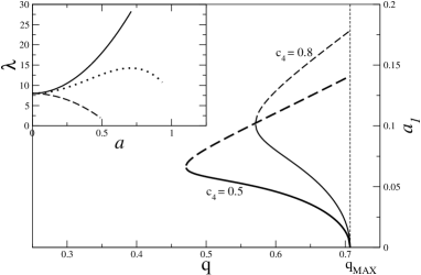
Figure 1: The amplitude of stationary solutions as function of $q$, for square symmetry ($2q^{2}_{\hbox{\tiny MAX}}=k^{2}_{\hbox{\tiny MAX}}=1$): the full line indicates the branch along which the system will coarsen; along the dashed line there is no coarsening. Branches marked by the thinnest line correspond to a larger value of $c_{4}$. Inset: the three possible scenarios for the growth model in 2D found in the limit $k\to k_{\hbox{\tiny MAX}}$, in which the sign of the diffusion coefficients that can give instability is linked to the behaviour of the amplitude $a$ with respect to the wavelength $\lambda$. We have coarsening (full line), no coarsening (dashed line), and interrupted coarsening (dotted line).

Coarsening scenarios and coarsening exponents.—Even if an exact determination of diffusion coefficients can only be done numerically, there are two crucial limits allowing analytical treatment: the small amplitude limit $(k\to k_{\hbox{\tiny MAX}}=1)$ and the large wavelenght/large amplitude limit. The former provides the proof of the existence of different coarsening scenarios, the latter provides the explicit values of coarsening exponents.

For the small amplitude limit, we have considered an isotropic current of the form $\mathbf{j}(\mathbf{m},c_{2},c_{4})=\mathbf{m}(1+c_{2}\mathbf{m}^{2}+c_{4}\mathbf{m}^{4})$ and we have found SM steady solutions and diffusion coefficients for both square and hexagonal symmetries. In both cases, the phase stability is controlled by the amplitude $a_{1}(q)$ of the steady state: we have instability, i.e. coarsening, if $a^{\prime}_{1}(q)<0$ (see Fig. 1). The sign of this derivative is determined by the coefficients $c_{2}$ and $c_{4}$: perpetual coarsening occurs if $c_{2}<0,c_{4}\leq 0$ (or $c_{2}>0,c_{4}<0$), no coarsening if $c_{2}>0,c_{4}>0$, coarsening up to a critical wavelenght (interrupted coarsening) if $c_{2}<0,c_{4}>0$. The basic three scenarios are illustrated in the inset of Fig. 1.

Perpetual coarsening is determined by a phase instability occurring for any $q$. In this case we can extract the coarsening exponent $n$, $L(t)\approx t^{n}$, through the following dimensional law:

$$|D(q)|\approx\frac{L^{2}}{t},$$ (17)

with $q=2\pi/L$. The application of Eq. (17) has always given values in agreement with known results, both in 1D 1d and in 2D 2d .

We insist on highlighting that the form of $\mathbf{j}$ is arbitrary and that here we shall only distinguish between two broad classes of systems: those which exhibit slope selection and those which do not. In the first case the current $\mathbf{j}(\mathbf{m})$ has zeros for finite values of the slope $\mathbf{m}^{*}$ (as, for example, with $\mathbf{j}=\mathbf{m}(1-\mathbf{m}^{2})$), so that pyramids will grow in size but with a slope tending to the constant value $\mathbf{m}^{*}$, leading to faceting. This implies that $\mathbf{m}^{*}=(\partial_{x}h_{0},\partial_{y}h_{0})$ is constant, except along domain walls, that have a finite but small thickness. We first consider the square symmetry, so, for example:

$$\langle h_{11}^{2}\rangle=\frac{1}{(2\pi)^{2}}\int_{0}^{\lambda}dx\int_{0}^{\lambda}dy\frac{1}{q^{2}}\left(\frac{\partial^{2}h_{0}}{\partial x^{2}}\right)^{2}=c_{11}\lambda^{3}+o(\lambda^{3})$$

where $c_{11}$ is a positive constant. With the same reasoning, at the leading order in $\lambda$ we find $\langle h_{12}^{2}\rangle=c_{12}\lambda^{3}$ and $\langle h_{1,2}^{2}\rangle=c_{\varphi}\lambda^{2}$. Therefore, we get $\displaystyle D_{11}=-2qc_{12}/c_{\varphi}$, that is negative, signaling instability. For the other coefficient we have $(D_{11}+D_{22}+D_{12})=2q(c_{12}-c_{11})/c_{\varphi}$, with $c_{11}>c_{12}$ for phase instability. Plugging the results for the $D_{ij}$’s into (17) we finally obtain:

$$L\sim t^{1/3}.$$ (18)

A similar analysis for hexagons allows us to determine (16) that has exactly the same behaviour with $\lambda$ as for the square symmetry, meaning that coarsening exponent $n=1/3$ also holds for 6-fold symmetry.

We have also analyzed the coarsening exponents for models without slope selection in the steady pattern: when $L$ increases, the slope increases as well. Assuming that the mound profile changes only along one direction while remains constant along the perpendicular one, we can find the asymptotic profile. Thus, for a current that behaves asymptotically (large slope) as $\mathbf{j}(\mathbf{m})\simeq 1/|\mathbf{m}|^{\beta}$, $\beta>1$, we have $\displaystyle 1/|\mathbf{m}|^{\beta}=-\partial^{2}m/\partial x^{2}$. By using its solution, we have finally obtained the result:

$$L\sim t^{1/4}$$ (19)

for both symmetries and for any values of $\beta$, as in the 1D case 1d .

Conclusions and discussion—Time and length scales of the emerging structure have been investigated within the phase diffusion notion, which has allowed to relate the growth dynamics to the properties of stationary solutions. The sign of the coefficients that dictate instability is related to some abstract function (see Eq. (15)) that depends on steady-state solutions. In the limit of small amplitude the abstract function coincides with the amplitude of the pattern. In this case three kinds of scenarios, namely perpetual coarsening, no coarsening, and interrupted coarsening, are possible. This is the first analytical evidence of such dynamical scenarios in 2D growth models.

As for the coarsening exponents, they deserve a special discussion. In fact, while the result (18) for a faceted 6-fold pattern and the result (19) for an unfaceted pattern agree with numerics and scaling considerations Golubovic1997 ; golub00 , the exponent $n=1/3$ for a faceted square pattern seems to be in contradiction with some numerics golub00 ; siegert98 , where a slower coarsening $n=1/4$ is reported. These authors argue that in the square case the coarsening dynamics may be slaved to the appearance of roof-tops siegert98 , a type of domain wall which is not present in a regular lattice of square pyramids, where only the so called pyramid edges appear note_dw . This type of dislocations, according to golub00 ; siegert98 , plays a major role in their numerical simulations, leading to a slowing of coarsening: $n=1/4$ instead of $n=1/3$. However, more recent results GolubReview show that such topological defects may or may not appear, depending on the explicit form of the slope dependent current. Therefore, from the point of view of numerical simulations, the faceted square case does not give a unique picture. We should also add that in golub00 ; siegert98 the square pattern was pointed out as metastable and therefore defect generation was required to overcome the metastability barrier, but we have shown exactly that the square pattern is linearly unstable with respect to phase fluctuations.

A theory of coarsening in the presence of topological defects is beyond the reach of the present study. However, our results support the idea that coarsening can take place via pyramid coalescence, without the assistance of defect generation. Therefore, since defect occurrence was found to slow down coarsening, our analysis might suggest that there always exists a faster channel for dynamics, i.e. without the intervention of topological defects. It would be an important future line of research to see whether the presence of defects or the lack thereof, is a fundamental ingredient for some specific equations, or rather does it depend on initial conditions, boundary conditions, system size, etc…

All these results have been established without evoking any specific form of the slope dependent current $\mathbf{j}(\mathbf{m})$, therefore pointing to the existence of a universality class. Furthermore, the results are independent of the considered symmetries: hexagons and squares. It would be an interesting task for future research to see whether or not this conclusion survives for the three other Bravais lattices (rectangular, rectangular centered and oblique). Finally, we point out that unstable growth on a (111) surface produces a 3-fold pattern, which does not fall within Bravais lattices. It is an open question to understand how such pattern can be analyzed within our approach.

A last word for experimental reults is appropriate. While the large variability of experimental values for $n$ review_Paolo ; 111 prevents from a quantitative comparison, our different dynamical scenarios for coarsening are well observed Cu100 ; Rh111 ; Pt111 .

Acknowledgements—CM thanks CNR for a Short-Term Mobility award from their International Exchange Program and CNES for financial support. Useful discussions with Matteo Nicoli are also acknowledged.

References

- (1) C. Misbah, O. Pierre-Louis and Y. Saito, Rev. Mod. Phys. 82, 981 (2010).
- (2) P. Politi and C. Misbah, Phys. Rev. E 73, 036133 (2006).
- (3) A. J. Bray, Adv. Phys. 43, 357 (1994).
- (4) J. J. Arenzon, A. J. Bray, L. F. Cugliandolo and A. Sicilia, Phys. Rev. Lett. 98, 145701 (2007).
- (5) C. Misbah and P. Politi, Phys. Rev. E 80, R030106 (2009).
- (6) P. Politi, G. Grenet, A. Marty, A. Ponchet and J. Villain, Phys. Rep. 324, 271 (2000).
- (7) S. J. Watson and S. A. Norris, Phys. Rev. Lett. 96, 176103 (2006).
- (8) R. Kohn and X. Yan, Commun. Pure Appl. Math. 56, 1549 (2003).
- (9) Bo Li, Nonlinearity 19, 2581 (2006).
- (10) M. Rost, J. Krug, Phys. Rev. E 55, 3952 (1997).
- (11) L. Golubović, Phys. Rev. Lett. 78, 90 (1997).
- (12) L.-H. Tang, P. milauer and D. D. Vvedensky, Eur. Phys. J. B 2, 409 (1998).
- (13) J. Villain, J. Phys. France 1, 91 (1991).
- (14) J.-K. Zuo and J. F. Wendelken, Phys. Rev. Lett. 78, 2791 (1997).
- (15) F. Tsui, J. Wellman, C. Uher and R. Clarke, Phys. Rev. Lett. 76, 3164 (1996).
- (16) M. Kalff, P. Smilauer, G. Comsa and Th. Michely, Surf. Sci. Lett. 426, 447 (1999).
- (17) T. Michely and J. Krug, Islands, mounds, and atoms: patterns and processes in crystal growth far from equilibrium (Springer, 2004).
- (18) M. Siegert, M. Plischke, Phys. Rev. E 53, 307 (1996).
- (19) P. Politi and J. Villain, in Surface Diffusion: atomistic and collective processes, Ed. M. C. Tringides (Plenum Press, 1997).
- (20) J. Stewart and N. Goldenfeld, Phys. Rev. A 46, 6505 (1992). F. Liu and H. Metiu, Phys. Rev. B 48, 5808 (1993).
- (21) D. Zwillinger, Handbook of differential equations. (Academic Press, 1998).
- (22) The scalar product is defined as .
-
(23)
Since the equality of mixed partials, it is preferable to define new diffusion coefficients
and to assume in the diffusion equations (9).(20) - (24) See Supplemental Material at http://link.aps.org/supplemental/… for the details of the small amplitude limit.
- (25) D. Moldovan and L. Golubović, Phys. Rev. E 61, 6190 (2000).
- (26) M. Siegert, Phys. Rev. Lett. 81, 5481 (1998).
- (27) A pyramid edge is a domain wall where only one component of the slope changes. A roof top is a domain wall where both components of the slope change.
- (28) A. Levandovsky and L. Golubović, Phys. Rev. B 69, 241402 (2004); L. Golubović, A. Levandovsky, and D. Moldovan, East Asian J. Appl. Math. 1, 297 (2011).