Following states in temperature in the spherical $s+p$-spin glass model

Abstract

In many mean-field glassy systems, the low-temperature Gibbs measure is dominated by exponentially many metastable states. We analyze the evolution of the metastable states as temperature changes adiabatically in the solvable case of the spherical $s+p$-spin glass model, extending the work of Barrat, Franz and Parisi [J. Phys. A 30, 5593 (1997)]. We confirm the presence of level crossings, bifurcations, and temperature chaos. For the states that are at equilibrium close to the so-called dynamical temperature $T_{d}$, we find, however, that the following state method (and the dynamical solution of the model as well) is intrinsically limited by the vanishing of solutions with non-zero overlap at low temperature.

Keywords:

1 Introduction

Predicting the dynamical behavior of a system from a calculation of static quantities is the basic goal of statistical mechanics, where we consider the static average over all configurations rather than the joint dynamics of all the atoms. A particularly important case, both in classical and quantum thermodynamics, is given by the dynamics after very slow variations of an external parameter so that the system remains in equilibrium. Such changes are said to be “adiabatic”.

In mean-field systems it takes an exponentially large time, in the size of the system, to escape from a metastable state. It is, thus, a well posed question to study the “adiabatic” evolution of each such metastable state. One simply needs to consider that the speed of change of the external parameter is very slow but independent of the system size.

In glassy mean-field systems, at low temperatures, there are exponentially many metastable states. The equilibrium solution in these systems can be described using the replica theory or the cavity method [1]. Adiabatic evolution of the states can be described using the Franz-Parisi potential [2, 3]. One fixes a reference equilibrium configuration at temperature $T_{e}$ and computes the free energy at temperature $T_{a}$ restricted to configurations sharing a given degree of similarity with the reference configuration. A distance can be defined in terms of the overlap of system configurations with the reference configuration and the constrained free energy is the Franz-Parisi potential. The adiabatic evolution of the metastable state, to which the reference configuration belongs, can, then, be represented by the set of local minima of the Franz-Parisi potential at the shortest distance from this configuration.

Krzakala and Zdeborova recently introduced a procedure for following states that focuses directly on the minimum of the Franz-Parisi potential and is more easily tractable from a computational point of view [4, 5]. The method has been applied to a number of glassy mean field systems including the fully connected Ising $p$-spin glass model, the diluted Ising $p$-spin model (XOR-SAT) or the random graph coloring. In all these systems, for $T_{e}$ below the dynamic arrest temperature $T_{d}$ and for $T_{a}$ low enough, the replica symmetric (RS) Franz-Parisi potential ceases to have a local minima correlated to the reference configuration. If the Franz-Parisi potential is, rather, evaluated using 1RSB, the correlation with the reference configuration vanishes at a temperature $T_{a}$ lower than the one for the RS case, though it still vanishes. It was hence hypothesized that introducing further steps of replica symmetry breaking a physical solution might eventually be found.

The current work is motivated by these findings and consists in the study of the adiabatic evolution of states in the spherical $s+p$-spin glass model with different competing $p$-body interaction terms, where an arbitrary level of replica symmetry breaking is relatively easily tractable [6, 7, 8, 9], and where, moreover, the dynamical behavior can be exactly solved [10, 11, 12, 13], and agrees with the results of the computation of the Franz-Parisi potential.

When following the evolution of the states in the spherical spin glass model as temperature is lowered we find once again the loss of correlation with the reference configuration. In this case, though, we are able to explicitly check that further levels of replica symmetry breaking do not preserve the correlation from vanishing. We will discuss the implications of such property throughout the paper and their possible connections to systems with discrete variables.

The rest of the paper is organized as follows. Section 2 describes the model we study in this paper and summarizes the static replica equations under different levels of replica symmetry breaking. Section 3 derives the equations for evolution of states with the aid of the results we obtain in fully connected Ising $p$-spin model. In Section 4, we report results of the state evolution, discuss their physical meaning and compare them with existing results. Finally, in Section 4.4, we discuss the vanishing of states under cooling at low temperature.

2 Model and its thermodynamics

In this paper we study the spherical 3+4 spin-glass model with ferromagnetic interaction (3+4-FM model) whose Hamiltonian is

$$\mathcal{H}=-\sum_{i_{1}<i_{2}<i_{3}}J^{(3)}_{i_{1},i_{2},i_{3}}\sigma_{i_{1}}\sigma_{i_{2}}\sigma_{i_{3}}\,-\sum_{i_{1}<i_{2}<i_{3}<i_{4}}J^{(4)}_{i_{1},i_{2},i_{3},i_{4}}\sigma_{i_{1}}\sigma_{i_{2}}\sigma_{i_{3}}\sigma_{i_{4}}$$ (1)

where the interactions $J^{(p)}_{i_{1},i_{2}\ldots i_{p}}$ are i.i.d random Gaussian variables of mean $S_{p}p!/N^{p-1}$ and variance $J^{2}_{p}p!/(2N^{p-1})$, and the spins $\sigma_{i}$ real variables satisfying the global spherical constraint

$$\sum_{i=1}^{N}\sigma_{i}^{2}=N\,.$$ (2)

This model is a particular case of the general spherical spin glass model with ferromagnetic interaction defined by the Hamiltonian

$$\mathcal{H}=-\sum_{p=2}^{M}\sum_{i_{1}<i_{2}<\ldots<i_{p}}J^{(p)}_{i_{1},i_{2}\ldots i_{p}}\sigma_{i_{1}}\sigma_{i_{2}}\ldots\sigma_{i_{p}}\,,$$ (3)

where several $p$-uples $(i_{1},i_{2}\ldots i_{p})$ of spins interacting via random Gaussian interactions $J^{(p)}_{i_{1},i_{2}\ldots i_{p}}$, with the mean and variance given above, are considered. It turns out that close to the transitions only the first two non-zero terms in the sum (3) are relevant [14, 15], and so one usually considers the Hamiltonian (3) where only two terms are retained. To indicate which terms are considered these models are referred as $s+p$-FM models.

The equilibrium properties of these models can be obtained using the, now standard, replica method to average over the disorder. We briefly remind here the replica solution of this model as introduced in [6, 7, 8, 9, 16]. Introducing replicas and averaging the partition function over the disorder yields the static free energy functional, which reads

$$-2\beta F(\beta) = 1+\ln 2\pi+\lim_{n\to 0}\frac{1}{n}G[{\bm{q},\bm{m}}]\ ,$$ (4)

$$G[{\bm{q},\bm{m}}] = \sum_{ab}^{1,n}g(q_{ab})+\ln\det\left({\bm{q}}-{\bm{m}}\otimes\bm{m}\right)+\sum_{a=1}^{n}h(m_{a})\ .$$ (5)

where

$$g(q)=\sum_{p}\frac{\mu_{p}}{p}q^{p}, \qquad\mu_{p}\equiv\frac{p\beta^{2}J_{p}^{2}}{2}\,,$$ (6)

$$h(m)=\sum_{p}\frac{\nu_{p}}{p}m^{p}, \qquad\nu_{p}\equiv 2p\beta S_{p}\,,$$ (7)

$\bm{q}=\{q_{ab}\}$ is the (symmetric) overlap matrix, $\bm{m}=\{m_{a}\}$ the magnetization vector in the replica space and $\otimes$ represents the outer product of vectors. The free energy $G[\bm{q},\bm{m}]$ must be evaluated at the solution of the saddle point equations

$$\frac{\partial G[\bm{m},\bm{q}]}{\partial q_{ab}}=0\ \ \quad a\neq b\,,$$ (8)

$$\frac{\partial G[\bm{m},\bm{q}]}{\partial m_{a}}=0.$$ (9)

When breaking the permutation symmetry among replicas an Ansatz is imposed on the structure of overlap matrix ${\bm{q}}$. For a generic $R$-steps of replica symmetry breaking [17] the matrix ${\bm{q}}$ is divided along the diagonal into successive boxes of decreasing size. In each box $q_{ab}$ is constant and takes the value, from larger to smaller boxes, $0\leq q_{0}<q_{1}<\ldots<q_{R}<q_{R+1}=1$. The saddle point equation are better written with the help of the two additional functions:

$$\Lambda(q)=g^{\prime}(q),\ \qquad\omega(m)=\frac{h^{\prime}(m)}{2}\,.$$ (10)

where the ”prime” denotes the derivative.

2.1 RS and 1RSB solutions

We first consider the case of no replica symmetry breaking $R=0$, the replica symmetric (RS) Ansatz. The free energy (4) then becomes:

$$-2\beta F(\beta)=1+\ln 2\pi+g(1)-g(q_{0})+\log(1-q_{0})+\frac{q_{0}-m^{2}}{1-q_{0}}+h(m)$$ (11)

while for the internal energy we have

$$e(\beta)=-T\,[g(1)-g(q_{0})]-\frac{T}{2}h(m).$$ (12)

The parameters $q_{0}$ and $m$ are obtained from the self-consistent equations:

$$\Lambda(q_{0})=\frac{q_{0}-m^{2}}{(1-q_{0})^{2}},\ \qquad\omega(m)=\frac{m}{1-q_{0}}\,.$$ (13)

The particular RS solution $m=q_{0}=0$ gives the paramagnetic solution.

The RS solution is stable if and only if

$$\Lambda^{\prime}(q_{0})(1-q_{0})^{2}<1\,.$$ (14)

This inequality is always satisfied for large enough temperature $T$. However as $T$ is lowered the RS solution may become unstable and replica symmetry must be broken. The type of replica symmetry breaking, that is the value of $R$, depends on the terms appearing in the sum (3). If we limit ourself to the case 3+4-FM than only one step of replica symmetry breaking is needed [13, 16], see also the Appendix, thus $R=1$ leading to the one-step RSB (1RSB) Ansatz. The free energy for 1RSB Ansatz reads:

$$-2\beta F(\beta) = g(1)-g(q_{1})+x\,\bigl{[}g(q_{1})-g(q_{0})\bigr{]}+\frac{1}{x}\ln\chi(q_{0})$$ (15)

$$\phantom{==}+\frac{x-1}{x}\ln\chi(q_{1})+\frac{q_{0}-m^{2}}{\chi(q_{0})}\,,$$

where

$$\chi(q_{1}) = 1-q_{1}\,,$$ (16)

$$\chi(q_{0}) = 1-q_{1}+x(q_{1}-q_{0})\,.$$ (17)

The parameter $x$, called replica symmetry breaking parameter, represents the fraction of states (replicas) with overlap $q_{1}$. Similarly for the 1RSB energy we have

$$e(\beta)=-T\Bigl{[}g(1)-g(q_{1})+x\,\bigl{[}g(q_{1})-g(q_{0})\bigr{]}\Bigr{]}-\frac{T}{2}h(m).$$ (18)

The order parameters $q_{1},q_{0},m,x$ are the solutions of the saddle point equations:

$$\Lambda(q_{0})=\frac{q_{0}-m^{2}}{\chi^{2}(q_{1})}\,,$$ (19)

$$\Lambda(q_{1})-\Lambda(q_{0})=\frac{q_{1}-q_{0}}{\chi(q_{1})\chi(q_{0})}\,,$$ (20)

$$\omega(m)=\frac{m}{\chi(q_{1})}\,$$ (21)

and the additional requirement of stationarity of $G[q_{0},q_{1},x,m]$ with respect to variation of $x$

$$g(q_{1})-g(q_{0})=-\frac{1}{x^{2}}\ln\left[\frac{\chi(q_{1})}{\chi(q_{0})}\right]+(q_{1}-q_{0})\left[\frac{q_{0}-m^{2}}{\chi(q_{0})^{2}}-\frac{1}{x\chi(q_{0})}\right].$$ (22)

The 1RSB solution is stable as long as

$$\Lambda^{\prime}(q_{1})\chi^{2}(q_{1})<1\,$$ (23)

and

$$\Lambda^{\prime}(q_{0})\chi^{2}(q_{0})<1$$ (24)

are satisfied.

In systems with discontinuous 1RSB, besides the thermodynamic phase transition the replica theory also predicts a dynamic 1RSB (d1RSB) transition. The d1RSB solution can be obtained in the framework of the replica calculation using (19)-(21) and a different equation in place of (22). The latter is the so-called marginality condition for dynamic arrest and requires that $q_{1}$ be marginally stable, that is

$$\Lambda^{\prime}(q_{1})=\frac{1}{(1-q_{1})^{2}}$$ (25)

that ensures that the characteristic time of the correlation function diverges at, and below, the transition. This condition can be derived in different ways: (i) requiring that the complexity functional counting excited metastable states is maximal [6, 18, 19], or, equivalently, (ii) imposing that the lowest stability eigenvalue of the replica solution tends to zero [6, 19]. Else, (iii) it can be obtained as a saddle point equation for the RS solution with $q=q_{1}$ sending the number of replicas $n\to 1$ rather than $n\to 0$ [2, 3, 20] or, eventually, (iv) directly solving the equilibrium dynamics [10, 9].

From the Legendre transform of (15) with respect to $\beta x$, the complexity functional can be computed as

$$2\Sigma(q_{1}) = x^{2}\frac{\partial\beta F}{\partial x}=-x^{2}\left[g(q_{1})-g(q_{0})\right]+x^{2}\Lambda(q_{0})(q_{1}-q_{0})$$

$$-x\frac{q_{1}-q_{0}}{\chi(q_{0})}-\ln\frac{\chi(q_{1})}{\chi(q_{0})}\,.$$

Using (20) and the definition of $\chi(q_{0})$ (17), $x$ can be eliminated and $\Sigma(q_{1})$ can be rewritten as

$$2\Sigma = -1+(1-q_{1})^{2}{\cal L}_{10}-\ln\left[(1-q_{1})^{2}{\cal L}_{10}\right]$$ (28)

$$-\left[\frac{1}{1-q_{1}}-(1-q_{1}){\cal L}_{10}\right]^{2}\left[g(q_{1})-g(q_{0})-\Lambda(q_{0})(q_{1}-q_{0})\right]\,,$$

$${\cal L}_{10} \equiv \frac{\Lambda(q_{1})-\Lambda(q_{0})}{q_{1}-q_{0}}\,,$$

where $q_{0}$ is eliminated in favor of $q_{1}$ using

$$\Lambda(q_{0})=(q_{0}-m^{2})(1-q_{1})^{2}{\cal L}_{10}\,.$$ (29)

2.2 The 3+4-FM model: phase diagram and complexity

In this section we shortly summarize some features of the spherical 3+4-FM spin glass model that will be employed to test the states following procedure in the rest of the paper. In the following we choose, without loss of generality, $S_{3}=S_{4}$ and $J_{3}=J_{4}$. The phase diagram is displayed in Fig. 1 and consists of three equilibrium phases separated by red lines. At high temperature $T$ and not too large $S_{4}$ the phase is paramagnetic (PM) with $q=m=0$, while at low $T$ and sufficiently small $S_{4}$ we have a spin glass (SG) phase of 1RSB type with $q_{0}=m=0$. For large $S_{4}$ the phase becomes ferromagnetic (FM) of RS type with both $m$ and $q$ positive. The transition to the FM phase is of first order, and the blue lines depict the spinodal lines of the FM and FM_1RSB –ferromagnetic of 1RSB type– metastable phases. Note that the FM_1RSB metastable phase goes continuously over a FM metastable phase, magenta line, before reaching the ferromagnetic transition. The SG transition is a discontinuous random first order transition, occurring at the Kauzmann temperature $T_{K}$, also called static temperature $T_{s}$, horizontal red line. We shall use both notations depending on the context. Finally the horizontal green line gives the dynamical transition that occurs at the higher dynamical transition temperature $T_{d}$, also called the mode coupling critical temperature.

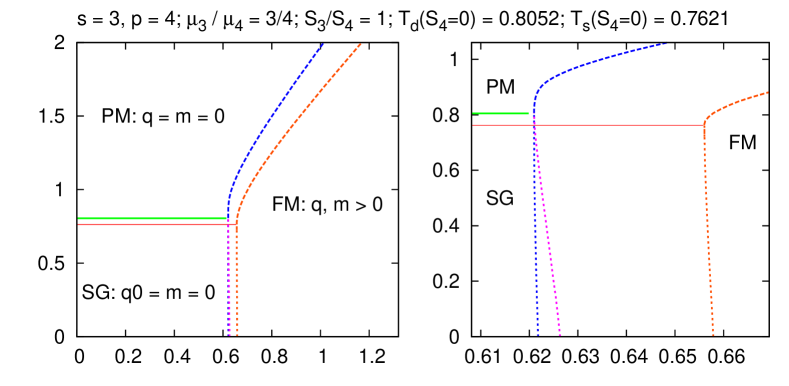
Figure 1: Phase diagram of the 3+4-FM spherical spin glass model with $J_{3}=J_{4}$ and $S_{3}=S_{4}$. The lines are: Red full: static PM/SG transition; green full: dynamic PM/SG transition; red dashed: PM/FM transition; red dotted: SG/FM transition; blue dashed: FM spinodal; blue dotted: FM_1RSB spinodal; magenta dotted: FM_1RSB/FM transition. The latter is hardly seen on the left panel. Right: Detail of the spinodal lines.

When the ferromagnetic FM_1RSB phase exists, its complexity, i.e., the logarithm of the number of metastable states, is extensive. We can then compare it with the complexity of the SG phase. The simplicity of the spherical model allows to plot them as function of $q_{1}$ only. This is done in Figure 2 where the behavior of $\Sigma(q_{1})$ versus $q_{1}$ is shown for three temperatures: $T<T_{K}$, $T=T_{K}$ and $T=T_{d}$. Not all values of $q_{1}$ correspond to physical solutions, i.e., satisfy Eq. (23): only the thick lines refer to the interval in which $\Sigma(q_{1})$ counts physical solutions. The thin lines counts solutions that are unstable in the replica space, and hence unphysical. One can notice that the order of magnitude of the complexity of the FM_1RSB is two orders of magnitude smaller than that of the spin-glass phase.

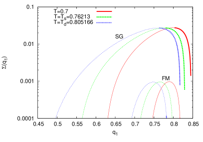
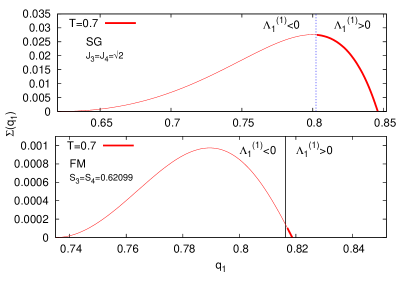
Figure 2: Left: Complexity curves versus $q_{1}$ for the spherical 3+4-FM spin glass model with $J_{3}=J_{4}$ and $S_{3}=S_{4}=0.62099$. Left: $\Sigma(q_{1})$ for $T=0.7$, $T=T_{k}=0.76213$ and $T=T_{d}=0.80517$ in the SG phase and in the FM_1RSB phase. Plot is in $y$-log scale to allow for comparison of complexity curves in both phases. Thick lines, hardly seen for the FM_1RSB phase, represent stable branches, thin lines unstable. Right: $\Sigma(q_{1})$ at $T=0.7$ for the SG states (top) and for the FM_1RSB states (bottom). Vertical lines denote the instability point.

3 Equations for evolution of states for $T_{e}\geq T_{K}$

In this section, we give the equations for adiabatic evolution of equilibrium states at $T_{K}\leq T_{e}\leq T_{d}$ in temperature $T_{a}$ following the planting procedure as introduced in Ref. [21]. We recall that the temperature $T_{K}$ (or $T_{s}$) is the so-called Kauzmann temperature at which a true static thermodynamic glass transition takes place, at least in mean-field systems, between a paramagnet and a thermodynamically stable equilibrium glass (the ideal glass). For simplicity, we only consider models with $S_{p}=0$.

For $\beta_{e}\geq\beta_{K}$ (that is, $T_{e}\leq T_{K}$), in order to select an equilibrium configuration, we, first, generate a configuration randomly and then construct all of the interaction constants $J_{i_{1},i_{2},\ldots,i_{r}}$ so that the energy of the planted configuration equals $e(\beta_{e})$, cf. Eq. (12). The important point is that, since above the Kauzmann temperature the RS quenched free energy is exactly the annealed free energy, the random planting ensemble is equivalent with the usual random ensemble, i.e. we can do a quiet planting [21, 22]. This is a very non trivial property: as long as $T>T_{K}$ when we generate a random configuration and a random set of interactions, so that this configuration is an equilibrium one, we have simply generated an equilibrated configuration of a typical realization of the usual random ensemble.

It seems difficult to plant an equilibrium configuration in the spherical spin models due to the fact that $\{\sigma_{i}\}_{i=1}^{N}$ are real variables which can range from $-\infty$ to $\infty$. However, the RS free energy of the spherical model with $S_{p}=0$ equals that of Ising model [5], which means that the Gibbs measure of spherical model is dominated by the Ising configurations $\{-1,1\}^{N}$. Consequently, for the spherical model, we can follow the same planting procedure as introduced in the Ising model in order to derive the equations of the evolution of states. We refer the reader to [22] for details, but the point is that for such models where RS quenched free energy is the annealed free energy, one can map the following state procedure to a usual static computation in a model with a ferromagnetic bias. We shall briefly recall how this can be done:

First, we generate a random configuration $\bf{\sigma}$ with $\sigma_{i}\in\{-1,1\}$. We then generate the (planted ensemble) interactions according to

$$P(J|{\bf{\sigma}})\propto e^{-\beta{\cal{H}}_{J}({\bf\sigma})}\prod_{ij}{\cal{N}}\left(J_{ij},0,\frac{J_{p}^{2}p!}{2N^{p-1}}\right),$$ (30)

where ${\cal N}(x,\bar{x},\Delta)$ is the normal distribution of mean $\bar{x}$ and variance $\Delta$. In doing so, we have generated a typical configuration of the planted ensemble, which is the same as the quenched one as long as $T>T_{K}$. In the annealed spherical model with $S_{p}=0$, the interaction variance scales as $\langle{J^{(p)}_{i_{1}\ldots i_{p}}}^{2}\rangle=J_{p}^{2}p!/(2N^{p-1})$, implying an extensive, $O(N)$, energy and, thus, from the central limit theorem, we have the typical value $J^{(p)}\sim J_{p}\sqrt{p!/(2N^{p-1})}$.

Call a $p$-interaction is satisfied (unsatisfied) if the energy contribution $J^{(p)}_{i_{1},i_{2},\cdots i_{p}}\sigma_{i_{1}}\sigma_{i_{2}}\cdots\sigma_{i_{p}}$ is negative (positive). Then, at inverse temperature $\beta_{e}$, we have the following expression for the fraction of unsatisfied interactions:

$$\epsilon^{(p)}=\frac{1}{2}+\frac{e(\beta_{e})}{J_{p}}\sqrt{\frac{p!}{2N^{p-1}}}$$ (31)

where $e(\beta_{e})$ is defined in (12). As we only consider $\beta_{e}\leq\beta_{K}$, in the model with $S_{p}=0$, it leads to $q_{0}=m=0$ and therefore,

$$\epsilon^{(p)}=\frac{1}{2}-\frac{\beta_{e}J_{p}}{2}\sqrt{\frac{p!}{2N^{p-1}}}.$$ (32)

We now use the fact that this configuration can be transformed to a uniform one (all $\sigma_{i}=1$) due to the Gauge invariance, i.e., for any spin $i$, the transformation $\sigma_{i}\to-\sigma_{i}$, $J_{a}\to-J_{a}$ (for all interactions $a$ involving spin $i$) will keep the Hamiltonian (3) invariant. Then, for all $p$, choose the signs of interactions in the $p$-interactions: $J_{i_{1},i_{2},\ldots,i_{p}}^{(p)}$, such that fraction $\epsilon^{(p)}$ of them is unsatisfied.

After this transformation is performed, we are left with the problem of finding where the uniform ”all up” configuration is an equilibrium one, and where the distribution of interactions is given by

$$P^{\mathrm{eff}}(J)\propto\prod_{ij}{\cal{N}}\left(J_{ij},\frac{S_{p}^{\mathrm{eff}}p}{N^{p-1}},\frac{J_{p}^{2}p!}{2N^{p-1}}\right),$$ (33)

with

$$S_{p}^{\mathrm{eff}}=\frac{\beta_{e}J_{p}^{2}}{2}.$$ (34)

In fact, (34) is exactly the Nishimori line condition for spherical $p$-spin spin glass model [5]. Therefore, for model with $S_{p}=0$ and for $T_{e}>T_{K}$, all of the thermodynamic properties of the states can be obtained from the phase diagram of the corresponding ferromagnetically biased model. In particular, since the planted configuration is an equilibrium one at $T_{e}$, we can rewrite the complexity function (i.e., the logarithm of the number of equilibrium thermodynamic states) at $T_{e}$ as following:

$$\Sigma(\beta_{e})=-\beta_{e}F(\{S_{p}=0\})+\beta_{e}F(\{S_{p}^{\mathrm{eff}}\})$$ (35)

from which we can determine the dynamical temperature $T_{d}$, i.e., the highest temperature at which Eq. (35) becomes positive, and the Kauzmann temperature $T_{K}$, at which Eq. (35) goes to zero. The reader interested in this correspondance between the following state procedure and the Nishimori line is referred to [21, 5, 22] for more details.

4 Results and discussion

In this section we present the results of adiabatic state following for the spherical 3+4-FM spin glass model with $J_{3}=J_{4}=1$, and $S_{3}=S_{4}=0$, we discuss their physical meaning and compare with the existing results.

4.1 Mapping to the phase diagram of the ferromagnetically biased model

By exploiting the equivalence between the evolution of states that were the equilibrium ones above $T_{K}$ and the thermodynamic properties of the model on the Nishimori line, we can acquire all the information about how states evolve with temperature from the phase diagram of the spherical 3+4-FM spin glass model discussed in Sec. 2.2 and plotted in Figure 1. Due to the Nishimori condition we will now have $S^{\rm eff}_{3}=S^{\rm eff}_{4}=\beta_{e}/2$. We show the phase diagram in the $T_{e}$, $T_{a}$ space in Figure 3, where the Nishimori line, given by $T_{e}=T_{a}$, is plotted as a black line: it intersects the spinodal transition line at the dynamical temperature $T_{d}$ and it exactly crosses the intersection of three phase transitions lines at the Kauzmann temperature, $T_{a}=T_{e}=T_{K}$. In the inset of Figure 3 we emphasize the re-entrant nature of the FM phase, comparing the borderline of the FM phase (red dotted) and the FM spinodal line (blue dotted) with vertical arrows, respectively at $T_{e}=T_{K}$ and $T_{e}=T_{d}$. The magenta line separates the FM and FM_1RSB (metastable) phases.

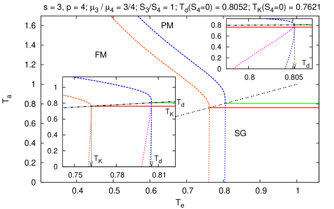
Figure 3: Phase diagram of the spherical 3+4-FM spin glass model as a function of temperature $T_{a}$, and $T_{e}$ $(2T_{e}=1/S^{\rm eff}_{4})$. Three thermodynamic phases are present separated by red lines: PM, SG an FM. The blue line is the spinodal line, while the green line is the dynamic PM/SG transition. For more details on the lines see Fig. 1. Note that both the FM phase transition and the spinodal line are reentrant, as emphasized in the insets. The metastable state that appears at the spinodal line is either FM or FM_1RSB. The magenta line denotes the transition between these two phases.

To interpret this phase diagram for the adiabatic evolution of Gibbs state we consider states that were at equilibrium at temperature $T_{e}$, $T_{K}\leq T_{e}\leq T_{d}$. The Nishimori line $T_{a}=T_{e}$ is hence the equilibrium line for $T_{e}>T_{K}$. As $T_{a}$ increases the states encounter the ferromagnetic spinodal (blue dash-dotted line) and “melt” into the paramagnet. As $T_{a}$ decreases there are three possible cases depending on the value of $T_{e}$ between $T_{K}$ and $T_{d}$, c.f.r. Figure 3. Starting from $T_{e}=T_{K}$, and increasing $T_{e}$, we have:

• For $T_{e}>T_{K}$, the state can be followed lowering $T_{a}$ using the RS Ansatz down to zero temperature.

• As $T_{e}$ becomes larger than the value where the FM/FM_1RSB transition line touches the $T_{a}=0$ axis, see Fig. 3, then the state can be followed using the RS Ansatz only down to a bifurcation temperature $T_{a}=T_{\rm 1RSB}$, where the crossing with the FM/FM_1RSB transition line occurs. Here the state splits into exponentially many sub-states with a 1RSB structure. This ensemble of states can be followed down to zero temperature using the 1RSB scheme.

• Finally when $T_{e}$ becomes larger than the value where the FM spinodal line touches the $T_{a}=0$ axis, the state can be followed as before with RS Ansatz down to $T_{\rm 1RSB}$, where the crossing with the FM/FM_1RSB transition occurs, and below this point with the 1RSB Ansatz. However at difference with the previous case we cannot reach $T_{a}=0$, but we have to stop at the temperature $T_{a}=T_{\rm spFM}$ where we cross the reentrant FM spinodal line. Below this temperature ferromagnetic solutions of any type do not exist anymore. Within the state following interpretation of the phase diagram this means that the state completely disappears, and hence no solution exists correlated with the state in equilibrium at $T_{e}$. The vanishing of states will be further discussed in section 4.4.

4.2 Evolution of states

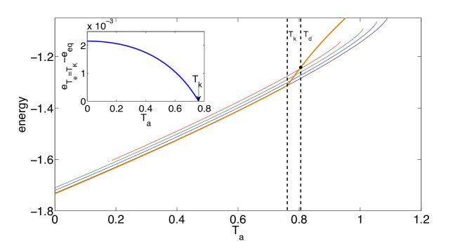
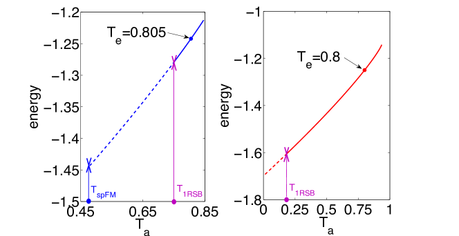
Figure 4: Evolution of states in spherical 3+4-FM spin glass model for $T_{K}\leq T_{e}\leq T_{d}$. Top: The RS result; the thick yellow curve is the equilibrium energy $e(T)$ in the model with $S_{3}=S_{4}=0$. Other curves are the evolution of energy of states with $T_{e}=0.805166(=T_{d}),0.8,0.785,0.773,0.76213(=T_{K})$, respectively. Notice that the equilibrium state at $T_{e}=T_{d}$ disappears as soon at $T_{a}<T_{e}$. Inset: Difference between the equilibrium energy of model and the energy of states of equilibrium at $T_{e}=T_{K}\approx 0.76213$. Bottom: The result for $T_{e}=0.805$ (left) and $T_{e}=0.8$ (right). The RS part is drawn in solid line and the 1RSB result in dashed line. For $T_{e}=0.805$ (left) the state following ends at $T_{\rm spFM}=0.4794$ where the reentrance of the FM spinodal line is reached.

Figure 4 shows how the energy of states evolves in temperature, compared with the equilibrium energy, thick yellow line in figure, from the 1RSB computation [19]. The top part of the figure shows the result of state evolution computed within the RS Ansatz from Eqs. (13), with $S_{p}$ given by $S_{p}^{\mathrm{eff}}$ defined in Eq. (34). Upon warming, the energy of the state grows up to a spinodal temperature beyond which the only solution is $(q_{0},m)=(0,0)$. As $T_{e}$ approaches $T_{d}$ from below, the energy of the spinodal point decreases gradually and goes to $e(T_{d})$ at $T_{e}\to T_{d}$. Note that this is not the case for the pure spherical $p$-spin spin glass model, where one retains only on term in the sum (3), which is kind of pathological in this aspect. The states at equilibrium at $T_{d}$ do not exist at any temperature higher than $T_{d}$. Upon cooling, the energy decreases. However, for $T_{e}$ close enough to $T_{d}$ the only RS solution of Eqs. (13) at low $T_{a}$ is the paramagnetic one.

The energy of states at equilibrium at $T_{e}=T_{K}$, followed at $T_{a}<T_{K}$, is different from the equilibrium energy and their difference is shown in the inset of Figure 4 (a). This indicates that these states fall out of equilibrium upon cooling, in contrast with the pure spherical $p$-spin spin glass models where the equilibrium state at $T_{e}=T_{K}$ is always at equilibrium for $T_{a}<T_{K}$. Thus, level crossing and temperature chaos do appear for $T_{e}<T_{K}$ in the spherical 3+4-FM spin glass model.

The lower part of Figure 4 shows the evolution of states computed with the 1RSB Ansatz, which is stable in this case [19]. The 1RSB solution, with $(m,q_{0})\neq(0,0)$ and $q_{1}\neq q_{0}$, corrects the RS result below the state splitting temperature $T_{\rm 1RSB}$. As illustrated on the left, for $T_{e}$ close enough to $T_{d}$ we encounter the reentrant spinodal line, below which no solution of the 1RSB equations is found with $m>0$, and the state following ends.

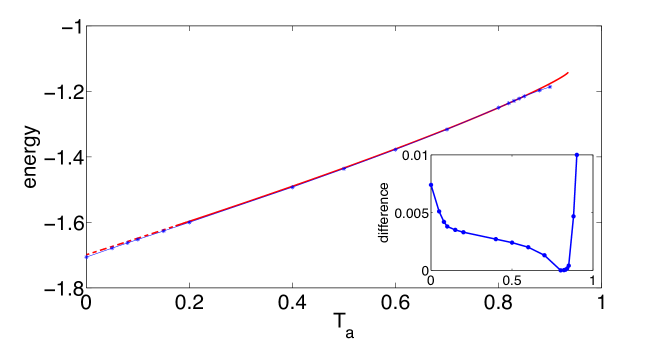
Figure 5: Comparison of the results derived from following states method (red line) and that from iso-complexity approach [23] (blue line with stars) where $T_{e}=0.8$. Inset: The difference between the two energies , $e_{\mathrm{exact}}-e_{\mathrm{iso}}$, as a function of $T_{a}$.

Finally, let us compare our results for adiabatic state following with an “iso-complexity” approximation proposed in Ref. [23] to study the cooling procedure in one state. In the iso-complexity approximation we count the logarithm of the number of the states at $T_{a}$ vs. energy and we choose the energy such that this number equals the equilibrium complexity at $T_{e}$. The true state following energy cannot be lower than the iso-complexity energy prediction, because, otherwise, there would not be enough states at $T_{a}$ at such lower energy, but it can be higher, since states that were not the equilibrium ones at $T_{e}$ can contribute to the complexity. We show in Figure 5 the energy of the state at equilibrium at $T_{e}=0.8$ at different $T_{a}$ computed using our exact method and the iso-complexity approximation. As we expect, the iso-complexity provides a lower bound to the true energy of the state (see the difference in the inset). This result is different from the case of the pure spherical $p$-spin spin glass model, in which the two methods give the same results because states do not cross or disappear.

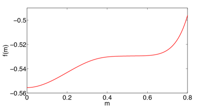
(a)

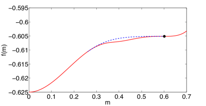
(b)

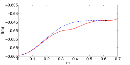
(c)

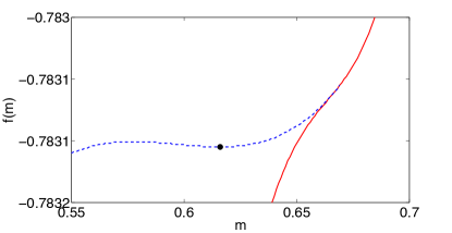
(d)

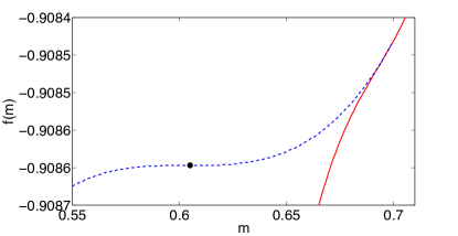
(e)

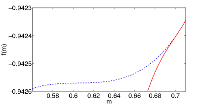
(f)

Figure 6: Free energy of a state at $T_{a}$ at a fixed overlap with a configuration at equilibrium at $T_{e}$. Here, $T_{e}=0.805$ and $T_{a}=0.9$ (a), $0.805$ (b), $T_{1RSB}=0.7525$ (c), $0.6$ (d), $T_{\rm spFM}=0.4794$ (e), $0.45$ (f), respectively. The solid red line represents the RS free energy and the dashed line the 1RSB free energy. The marks indicate the minimum of the free energy.

4.3 Relationship with Franz-Parisi potential

The results presented in the previous sections are equivalent to the results of Ref. [24]. The Franz-Parisi potential measures the free energy at temperature $T_{a}$ of the system at fixed overlap with a solution sampled from equilibrium at temperature $T_{e}$. Under our planting mechanism, magnetization is exactly the overlap between the configuration in the state of equilibrium at $T_{e}$ and the typical configuration in the same state at $T_{a}$; therefore, the free energy of the model with a ferromagnetic bias at a fixed magnetization can be directly translated into the Franz-Parisi potential.

Figure 6 shows the Franz-Parisi potential for the spherical 3+4-FM spin glass model with $S^{\rm eff}_{4}=\beta_{e}/2$, i.e., the free energy of the configurations linked to that at the equilibrium temperature $T_{e}$, versus the magnetization $m$ for $T_{e}=0.805$, close to $T_{d}$, and different $T_{a}$. The position on the cooling path is shown in the left panel of Figure 7, where the displayed temperatures $T_{a}$ are indicated by points. The right panel of Figure 7 shows the value of the parameters $q,q_{0},q_{1},m,x$ along the cooling path from $T_{a}=T_{e}=0.805$ down to $T_{a}=T_{\rm spFM}=0.4794$. For $T_{a}>T_{s}$, Figure 6 (a), the Franz-Parisi potential does not have any secondary minimum at $m>0$ besides the one at $m=0$. When $T_{\rm 1RSB}<T_{a}<T_{s}$, see Figure 6 (b), a secondary local minimum at $m^{\star}>0$ develops in the RS potential. At $T_{\rm 1RSB}=0.7525$, see Figure 6 (c), this minimum becomes unstable towards 1RBS, the dashed part of the curves. When cooling further, the minimum in RS free energy disappears, while it still exists for the 1RSB free energy, see Figure 6 (d). The latter disappears when the reentrance of the FM spinodal is reached for $T_{a}=T_{\rm spFM}=0.4794$, see Figure 6 (e), and beyond this point the Franz-Parisi potential ceases to have a minimum for $m>0$, see Figure 6 (f). These results are equivalent to those of Ref. [24], though there the case represented in Figure 6 (f) was not considered.

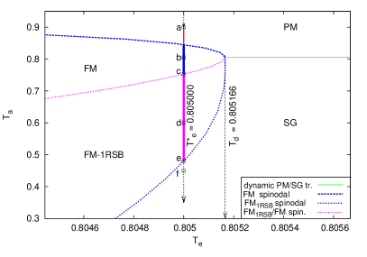
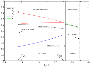
Figure 7: Left: Zoom into the $T_{a}$, $T_{e}$ phase diagram. The cooling path at $T_{e}=0.805$ is denoted by the full-line. The temperatures $T_{a}$ shown in Fig. 6 are indicated by squares. Right: The magnetization $m$ (black solid line) and the parameters $q$ (RS) and $q_{0}$, $q_{1}$ and $x$ (1RSB) as function of $T_{a}$ along the cooling path $T_{e}=0.805$. The magnetization $m$ coincides with the local minimum $m^{\star}$ of the free energy shown in Fig. 6. In the FM phase the overlap $q$ (green solid line) increases when cooling down and splits into $q_{0}$ and $q_{1}$ (red lines) when the (continuous) transition to the the FM_1RSB phase is reached. The breaking parameter $x$ (blue line) is, discontinuous, and jumps from zero to a finite value. The metastable FM_1RSB solution eventually disappears at $T_{\rm spFM}=0.4794$ and below this point no ferromagnetic solution exists.

4.4 A loose end in the following states

Starting from the equations for the Langevin dynamics, authors of Ref. [24] and Ref. [25] derive explicitly the adiabatic evolution of order parameters for the spherical 3+4-FM spin glass model, see Equation (25)-(26) in [24] or Equation (12) in Ref. [25] (notice that there $J_{4}=0.45J_{3}$ as chosen rather than $J_{4}=J_{3}$). These equations are exact description of the dynamics for $T_{a}>T_{\rm 1RSB}$ (denoted $T_{\rm ag}$ in Ref. [25]).

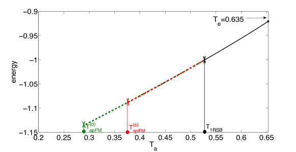
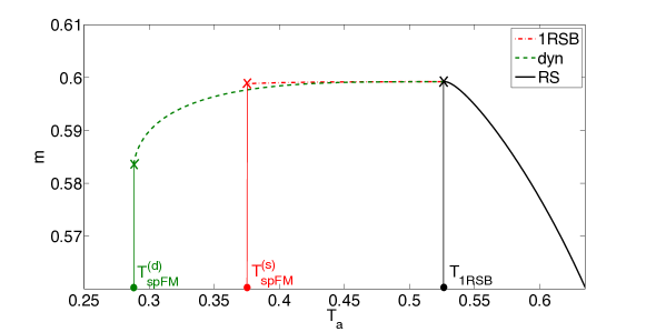
Figure 8: Energy (top) and magnetization $m$ (bottom) as function of $T_{a}$ along the path $T_{e}=0.653$ for the spherical 3+4-FM spin glass model with $J_{3}=1$, $J_{4}=0.45$ (to compare with results of Ref. [25]). At $T_{a}=T_{\rm 1RSB}$ the RS solution becomes unstable and the FM_1RSB appears. Red: results from the following states method, Green: results from the approximate dynamic solution of Ref. [24, 25]. The following of states ends at the $T_{\rm spFM}^{(s)}=0.355$ and $T_{\rm spFM}^{(d)}=0.288$, respectively, where the corresponding spinodal lines are reached. The energies of the two different method are almost indistinguishable, however but $E^{(s)}<E^{(d)}$.

For $T_{a}<T_{\rm 1RSB}$ the dynamical solution of [24, 25] is approximate because aging appears within states for such temperatures. The dynamical equations they obtain are the same as our 1RSB equations (19)-(21), and also coincide with stationarity of Franz-Parisi potential function with respect to $q_{1}$,$q_{0}$ and $m$. The stationary condition (22) is, however, replaced by the marginal condition (25), as expected from a dynamical calculation.

We then conclude that also the dynamical solution provided in Ref. [25] disappears because of the reentrance in the phase diagram of the spinodal line in the spherical 3+4-FM spin glass model, although at temperature $T_{\rm spFM}^{\rm(d)}$ slightly lower than the reentrant spinodal $T^{\rm(s)}_{\rm spFM}$ found from the static calculation. We plot the corresponding energy in the top panel of Figure 8. The bottom panel Figure 8 shows the value of $m$ for the two solutions. The vanishing states at low temperature was not noticed in Refs. [24, 25], because the data were for higher temperatures.

The disappearing of the states at the spinodal line rises the question of what may happen below this point. In the model we have studied the state, indeed, disappears. Therefore, the true long-time dynamics would completely de-correlates from the initial configuration ($m=0$). We are unable, so far, to predict at which energy the long-time dynamics will go from this point: this is a fundamental limit of the following state approach. It would be interesting to see if another approach allows to infer the long-time dynamics.

An interesting question is whether this behavior will be seen in other models with discrete, rather than continuous, variables. In fact, states vanishing seems to appear in many models, including the Ising counter-part of the $p$-spin model. However at low temperature the phase space of fully connected Ising models is more complex and is described by a FRSB Ansatz. This opens the question of the interplay between the state following method and the complexity of phase space. Hopefully, this can be studied along the line of the spherical case here presented.

Another direction to study the fate of the states at temperature $T_{\rm spFM}$ is to perform long and slow Monte-Carlo simulations starting from an equilibrated configuration (this can be achieve using the planting trick [21, 22]). We view these questions as an important open problem in the replica theory and pointing this clearly out is one of the main aims of this article.

5 Conclusion

In this paper, we study the adiabatic evolution of states that are at equilibrium at some temperature $T_{e}$ ($T_{K}\leq T_{e}\leq T_{d}$) in the spherical 3+4-FM spin glass model. We stress that while the study was performed for the 3+4-FM spin glass model, the results are generic for all $s$+$p$-FM spin glass model with only 1RSB low temperature phase.

After introducing the idea of planting an equilibrium configuration, the following states problem is mapped to the physics of the ferromagnetic solution in the corresponding model with a ferromagnetic bias, i.e., the model along the Nishimori line. We exactly describe the evolution of states away from equilibrium upon heating and cooling. This method is equivalent to the one based on the Franz-Parisi potential [24]. Within our mapping the Franz-Parisi potential is the free energy at fixed magnetization. Our method also reproduces the known results about the long time dynamics which is solvable for the spherical $p$-spin spin glass model [25].

The most interesting outcome of this paper is identification of a sort of boundary in the state following method and, hence, also in the Franz-Parisi potential and the dynamical solution for the spherical 3+4-FM spin glass model. We show that it is related to a reentrant behavior of spinodal lines in the phase diagram. For the states that are at equilibrium close to the dynamic transition temperature, we found that below a low but finite temperature, where we cross the reentrant spinodal line, no solution with a finite magnetization occurs, i.e., the correlation with the initial state at equilibrium is completely, and discontinuously, lost. In the spherical 3+4-FM spin glass model no physical solution with more than one step RSB takes place, thus no further fragmentation of states can be accounted to remove the reentrance: the states simply stop to exist. This leaves the following questions for future work: (1) Below the reentrance the following state method, or equivalently the Franz-Parisi potential, is unable to tell where and at which energy the dynamics will end. Is there a way to perform a static computation answering this question? (2) In the first part (RS) of the following state, the phase space is relatively simple and decreasing $T_{a}$ just constraints the system closer to the reference state and $m$ increases (in the ferromagnetic notation). This lasts until we reach the FM/1RSB transition where the phase space breaks down and becomes more complex. From this point on it becomes harder to stay close the reference state because the different states in which the phase space is broken into evolves chaotically (chaos in temperature). What happens beyond the FM/1RSB transition is thus an important point to study further. (3) Is the behavior similar in the Ising models? While the RS and the 1RSB solution both display a reentrance, other solutions breaking the replica symmetry can exist and be self-consistent for discrete spin systems at low temperature, so it is possible to conceive that the reentrance shrinks and disappears allowing to follow states down to zero temperature. This is again an important point to study further.

The answer to all those question is calling for more detailed simulation of the Ising case, and more analytical studies. We hope that this article will motive future attention and work in these directions.

Appendix

In this section, we recall the general condition that ensures whether solutions with $R$-RSB ($R>0$) can exist. This proof has already been presented, see [6, 13], and it is reported here for completeness For any $R$ (including $\infty$) the functional $G[\bm{q},\bm{m}]$ (5) can be written as

$$\frac{1}{n}G[{\bm{q}},\bm{m}]=\int_{q_{0}}^{1}\!dq\,x(q)\,\Lambda(q)+\int_{q_{0}}^{q_{R}}\!\frac{dq}{\chi(q)}+\ln\left(1-q_{R}\right)+\frac{q_{0}-m^{2}}{\chi(q_{0})}+h(m)\,,$$

(36)

where the function

$$x(q)=p_{0}+\sum_{r=0}^{R}(p_{r+1}-p_{r})\theta(q-q_{r})$$ (37)

is the cumulative probability density of the overlaps, $p_{r}$ ($p_{0}=n$ and $p_{R+1}=1$) are the sizes of the blocks along the diagonal and $q_{r}$ the value of $q_{ab}$ in the block, and

$$\chi(q)=\int_{q}^{1}\!dq^{\prime}~{}x(q^{\prime}).$$ (38)

For what concerns Replica Symmetry Breaking, only the overlap variables are involved and not single replica index parameters, such as magnetization $m_{a}$. Stationarity of the free energy functional with respect to $q_{r}$ and $p_{r}$ leads, respectively, to the the self-consistency equations than can be concisely written as

$${\cal F}(q_{r})=0,\qquad\qquad r=0,\ldots,R,$$ (39)

$$\int_{q_{r-1}}^{q_{r}}dq~{}{\cal F}(q)=0,\qquad r=1,\ldots,R,$$ (40)

where

$${\cal F}(z)\equiv\Lambda(z)-\int_{0}^{z}\!\frac{dq}{\chi(q)^{2}}.$$ (41)

Eq. (40) implies that ${\cal F}(q)$ has at least one root in each interval $[q_{r-1},q_{r}]$, that, however, is not a solution of (39). Following Ref. [13], we, then, observe that (39)-(40) guarantee that between any pair $[q_{r-1},q_{r}]$ there must be at least two extremes of ${\cal F}(q)$. Denoting the extremes by $q^{\star}$, the condition ${\cal F}^{\prime}(q^{\star})=0$ leads to the equation, cf. Eq. (41),

$$\chi(q^{\star})\equiv\int_{q^{\star}}^{1}x(q)~{}dq=\frac{1}{\sqrt{\Lambda^{\prime}(q^{\star})}},$$ (42)

where

$$\Lambda^{\prime}(q)=\frac{d\Lambda(q)}{dq}=\sum_{p}(p-1)\mu_{p}q^{p-2}.$$ (43)

Since $x(q)$ is a non-decreasing function of $q$, cf. (37), $\chi(q)$ is convex. The convexity of the function $[\Lambda^{\prime}(q)]^{-1/2}$ depends, instead, on the given values of multi-body interaction $g(p)$ considered, i.e., on the specific model, as well as on the parameters $\mu_{p}$, i.e. on the phase diagram point of interest. Non-zero values of the magnetization will affect the actual value of $q_{0}$, it will be $q_{0}>0$ for $m\not=0$, but it will not change the above argument since it only affects the values of $q$ at which $\chi(q)$ displays steps, but not the convexity properties of the function.

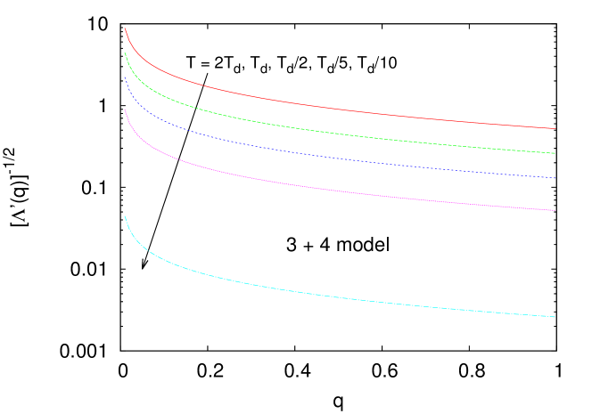
Figure 9: Right hand side of (42) for $J_{3}=J_{4}=1$ and $T=2T_{d},T_{d},T_{d}/2,T_{d}/5,T_{d}/10$, $T_{d}=0.805166$. As explained in text, the 3+4 curves never change convexity in any point of the phase diagram and can have no more than two intersections with $\chi(q)$ ($q_{0}$ and $q_{1}$), implying at most a 1RSB solution.

The $[\Lambda^{\prime}(q)]^{-1/2}$ for the 3+4 model that we deal with throughout this paper, is plotted in Figure 9 in different points of the phase diagram. The shape of $[\Lambda^{\prime}(q)]^{-1/2}$, concave, implies that at most a 1RSB solution can take place, excluding, among others, also any solution with a continuous RSB. This argument can be extended to show that 1RSB will be the most complicated solution for all $s+p$ systems in which $[\Lambda^{\prime}(q)]^{-1/2}$ never becomes convex for $q\in[0:1]$. Given a value of $s$ (equivalently of $p$) value this is quantitatively translated in satisfying the condition $p<p^{*}(s)$ ($s<s^{*}(p)$), where $p^{*}$ (or $s^{*}$) is solution of

$$(p^{2}+p+s^{2}+s-3sp)^{2}-ps(p-2)(s-2)=0$$ (44)

at fixed $s$ (or $p$), e.g., $(s^{*},p^{*})=(3,8)$, $(4,7+2\sqrt{6})$, $(5,9+3\sqrt{5})$.

References

References

- [1] Mézard M, Parisi G and Virasoro M A 1987 Spin-Glass Theory and Beyond (Lecture Notes in Physics vol 9) (Singapore: World Scientific)
- [2] Franz S and Parisi G 1995 Journal de Physique I 5 1401–1415
- [3] Franz S and Parisi G 1997 Phys. Rev. Lett. 79 2486–2489
- [4] Krzakala F and Zdeborová L 2010 EPL 90 66002
- [5] Zdeborová L and Krzakala F 2010 Phys. Rev. B 81 224205
- [6] Crisanti A and Sommers H J 1991 Zeitschrift fur Physik B Condensed Matter 87 341–354
- [7] Nieuwenhuizen T M 1995 Phys. Rev. Lett. 74 4289
- [8] Crisanti A and Leuzzi L 2004 Phys. Rev. Lett. 93 217203
- [9] Crisanti A and Leuzzi L 2007 Phys. Rev. B 76 184417
- [10] Crisanti A, Horner H and Sommers H J 1993 Zeitschrift fur Physik B Condensed Matter 92 257
- [11] Cugliandolo L F and Kurchan J 1993 Phys. Rev. Lett. 71 173
- [12] Barrat A 1997 The p-spin spherical spin glass model cond-mat/9701031
- [13] Crisanti A and Leuzzi L 2007 Phys. Rev. B 75 144301
- [14] Götze W and Sjörgen L 1989 J. Phys.: Condens. Matter 1 4203–422
- [15] Crisanti A and Ciuchi S 2000 Europhys. Lett. 49 754–760
- [16] Crisanti A and Leuzzi L 2012 in preparation
- [17] Parisi G 1980 J. Phys. A Lett. 13 L115–L121
- [18] Crisanti A, Leuzzi L and Rizzo T 2003 Eur. Phys. J. B 36 129
- [19] Crisanti A and Leuzzi L 2006 Phys. Rev. B 73 014412
- [20] Crisanti A 2008 Nucl. Phys. B 796 425
- [21] Krzakala F and Zdeborová L 2009 Phys. Rev. Lett. 102 238701
- [22] Krzakala F and Zdeborová L 2011 J. Chem. Phys. 134 034513
- [23] Montanari A and Ricci-Tersenghi F 2004 Phys. Rev. B 70 134406
- [24] Barrat A, Franz S and Parisi G 1997 J. Phys. A 30 5593–5612
- [25] Capone B, Castellani T, Giardina I and Ricci-Tersenghi F 2006 Physical Review B 74 144301
- [26] Gardner E 1985 Nuclear Physics B 257 747–765