Compensation effect in carbon nanotube quantum dots coupled to polarized electrodes in the presence of spin-orbit coupling

Abstract

We study theoretically the Kondo effect in carbon nanotube quantum dot attached to polarized electrodes. Since both spin and orbit degrees of freedom are involved in such a system, the electrode polarization contains the spin- and orbit-polarizations as well as the Kramers polarization in the presence of the spin-orbit coupling. In this paper we focus on the compensation effect of the effective fields induced by different polarizations by applying magnetic field. The main results are i) while the effective fields induced by the spin- and orbit-polarizations remove the degeneracy in the Kondo effect, the effective field induced by the Kramers polarization enhances the degeneracy through suppressing the spin-orbit coupling; ii) while the effective field induced by the spin-polarization can not be compensated by applying magnetic field, the effective field induced by the orbit-polarization can be compensated; and iii) the presence of the spin-orbit coupling does not change the compensation behavior observed in the case without the spin-orbit coupling. These results are observable in an ultraclean carbon-nanotube quantum dot attached to ferromagnetic contacts under a parallel applied magnetic field along the tube axis and it would deepen our understanding on the Kondo physics of the carbon nanotube quantum dot.

I Introduction

The experimental and theoretical studies of the Kondo effect Kondo1964 in artificial confined systems has attracted much attention since 1998, the first experimental observation of the Kondo effect in semiconductor quantum dot. Gordon1998 ; Cronenwett1998 ; Schmid1998 The advantage of the quantum dot as the platform studying the Kondo effect is its tunability, namely, one can tune readily the voltages of various electrodes of the quantum dot to control the relevant model parameters in describing the Kondo effect, as a result, one can study in a deep way various aspects of the transport property in such a system. For example, by tuning the gate voltage one can observe the Coulomb blockade effect, Meirav1990 ; Meir1991 the Kondo effect Gordon1998 ; Cronenwett1998 ; Schmid1998 and its unitary limit, Wiel2000 ; Delft2000 and even from the Kondo regime to the mixed-valence regime. Gordon1998b The non-equilibrium Kondo effect has also been studied by tuning the source-drain bias Simmel1999 ; Franceschi2002 and the couplings to the leads has been tuned to observe the offset of the Kondo resonance, Simmel1999 and so on.

Recently, due to the development of the spintronics the influence of the polarized electrodes attached to the quantum dot has also been intensively investigated experimentally Pasupathy2004 ; Hamaya2007 ; Sahoo2005 ; Hofstetter2010 and theoretically. Zhang2002 ; Sergueev2002 ; Martinek2003a ; Martinek2003b ; Sindel2007 ; Krawiec2007 ; Lim2010 ; Choi2004 ; Barnas2006 It was found that the effect of the polarized electrodes is equivalent to an effective exchange field and can be compensated by applying an external magnetic field. Pasupathy2004 ; Hamaya2007 ; Martinek2003a ; Martinek2003b ; Sindel2007 ; Krawiec2007 ; Lim2010

The semiconductor quantum dot involved only one level is a simple system to study the Kondo physics since in such a system only the spin degree of freedom is involved. A slightly complicated system involved degree of freedom other than the spin is the carbon nanotube (CNT) quantum dot, which includes the orbital degree of freedom, Ando2000 ; Nygard2000 ; Minot2004 ; Herrero2005 ; Choi2005 ; Makarovski2005 and the spin-orbit coupling could be stronger than the believed earlier, as predicted theoretically Hernando2006 ; Bulaev2008 and confirmed by the experiment. Kuemmeth2008 The presence of the spin-orbit coupling has a significant influence to the transport behaviors in the CNT quantum dot, for example, the $SU(4)$ symmetry discussed in the CNT quantum dot Herrero2005 ; Choi2005 is no longer valid and correspondingly the Kondo resonance shows some interesting splitting effects.Fang2008 ; Galpin2010 This motivates us to further study a question, namely, how does the compensation effect observed in the semiconductor quantum dot behave in the CNT quantum dot in the presence of strongly spin-orbit coupling? In Ref. [Lim2011, ], the Kramers polarization due to the presence of the spin-orbit coupling and its influence on the Kondo peak splitting have been studied in detail by using scaling analysis and the slave-boson technique. Guillou1995 ; Krawiec2007 The compensation effect of the $SU(2)$ spin and the orbital Kondo effects were discussed in the absence of the spin-orbit coupling. In the present work, we study systematically the compensation effect with and without the spin-orbit coupling and the results show many novel features as presented later.

Experimentally, the spin polarized transport through CNT quantum dots attached to ferromagnetic leads has been reported in the literature. Hauptmann2008 When the external magnetic field is applied perpendicularly, Hauptmann et. al. found that the exchange field can be compensated by the external field applied, which is consistent with that observed in the semiconductor quantum dot. The possible reason is that in the perpendicular case the spin projection along the CNT axis is no longer a good quantum number and as a result the response of the single-particle energy spectrum to the applied field is approximately the Zeeman effect-like. Logan2009 ; Fang2010 This is because that the perpendicular field only couples to the spin, not to the orbital degrees of freedom. In the present work we focus on the parallel magnetic field case, in which the presence of the strong spin-orbital coupling should play a significant role in the transport properties with the polarized electrodes.

There are three kinds of possible polarizations of conduction electrons in CNT, namely, the spin-polarization, the orbit-polarization and the Kramers polarization. Lim2011 In the absence of the spin-orbit coupling, the Kramers polarization is also absent. Thus we discuss the effects of the spin- and orbit-polarizations and compare them with those in the semiconductor quantum dots. In the presence of the spin-orbit coupling, the Kramers polarization is found to have a different feature in comparison to the spin- and orbit-polarizations. When both spin- and orbit-polarizations remove the degeneracy, the Kramers polarization can enhance the degeneracy. By applying magnetic field, the compensation behavior obtained is quite different to that found in the semiconductor quantum dot and in the perpendicular field case. While the effective exchange field induced by the orbit-polarization can be compensated, the effective exchange field induced by the spin-polarization can not be compensated. Due to the interplay between the spin-orbit coupling, the polarized electrodes (spin-, orbit- and Kramers polarizations) and the magnetic field applied, the Kondo peaks show complicated splitting behaviors. We analyze in detail the correspondences between these sub-peaks and their microscopic tunneling processes.

This paper is organized as follows. In Sec. II we use the Anderson model to describe the CNT quantum dot and use the Green’s function formalism to study the polarized transport behaviors. In Sec. III we present the explicit numerical results and discuss microscopic tunneling processes. Finally, Sec. IV is devoted to a brief summary.

II Model and Green’s function formalism

The CNT quantum dot can be described by the Anderson impurity model Anderson1961

$$H=\sum_{km\alpha}\epsilon_{km\alpha}c_{km\alpha}^{\dagger}c_{km\alpha}+\sum_{m}\varepsilon_{m}d_{m}^{\dagger}d_{m}+\frac{U}{2}\sum_{m\neq m^{\prime}}n_{m^{\prime}}n_{m}$$

$$\hskip 85.35826pt+\sum_{km\alpha}\left(V_{\alpha}d_{m}^{\dagger}c_{km\alpha}+h.c.\right),$$ (1)

where $d_{m}^{\dagger}(d_{m})$ and $c_{km\alpha}^{\dagger}(c_{km\alpha})$ represent the creation (annihilation) operators of an electron in the dot and the left ($\alpha=L$) and the right ($\alpha=R$) leads, respectively. Here $m=\{\sigma,\tau\}$ describes the configuration of electrons where $\sigma=\uparrow$ or $\downarrow$ and $\tau=\pm$ denote the spin and orbital quantum numbers. $\epsilon_{km\alpha}$ is the single-particle energy spectrum in the leads with the configuration $m$ and $\varepsilon_{m}$ is the dot level related to the spin-orbit coupling, which will be given below. $n_{m}=d_{m}^{\dagger}d_{m}$ is the occupation operator, $U$ is the on-site interaction and $V_{\alpha}$ is the tunneling amplitude between the dot and leads. Here we assume that the configuration $m$ of an electron is conserved during tunneling between the dot and leads.

The electronic structure of the dot affects directly its transport properties obtained from the current through the dot within the framework of the Keldysh formalism Meir1993 ; Jauho1994

$$I=\frac{i\,e}{\hbar}\frac{\Gamma_{L}\Gamma_{R}}{\Gamma_{L}+\Gamma_{R}}\sum_{m}\int\,d\omega\rho_{d,m}(\omega)\left(f_{L}(\omega)-f_{R}(\omega)\right),$$ (2)

where $f_{\alpha}(\omega)$ is the Fermi distribution of the lead $\alpha$ and $\Gamma_{\alpha}=\sum_{m}\Gamma_{\alpha,m}$ with $\Gamma_{\alpha,m}=\pi\rho^{0}_{\alpha,m}|V_{\alpha}|^{2}$. Here $\rho^{0}_{\alpha,m}$ denotes the density of states of the polarized electrodes with the configuration $m$, which is related to the spin polarization $P^{s}_{\alpha}$, the orbital polarization $P^{o}_{\alpha}$ as well as the Kramers polarization $P^{k}_{\alpha}$ in the presence of strongly spin-orbit coupling. Lim2011 Thus the coupling matrix of different configurations can be expressed as follows

$$\Gamma_{\alpha,\{\uparrow,+\}}=\frac{\Gamma_{\alpha}}{4}(1+P^{s}_{\alpha}+P^{o}_{\alpha}+P^{k}_{\alpha})$$ (3)

$$\Gamma_{\alpha,\{\uparrow,-\}}=\frac{\Gamma_{\alpha}}{4}(1+P^{s}_{\alpha}-P^{o}_{\alpha}-P^{k}_{\alpha})$$ (4)

$$\Gamma_{\alpha,\{\downarrow,+\}}=\frac{\Gamma_{\alpha}}{4}(1-P^{s}_{\alpha}+P^{o}_{\alpha}-P^{k}_{\alpha})$$ (5)

$$\Gamma_{\alpha,\{\downarrow,-\}}=\frac{\Gamma_{\alpha}}{4}(1-P^{s}_{\alpha}-P^{o}_{\alpha}+P^{k}_{\alpha})$$ (6)

In Eq. (2) $\rho_{d,m}(\omega)=-\frac{1}{\pi}\text{Im}G^{r}_{d,m}(\omega)$ is the density of states in the quantum dot, where the retarded Green’s function $G^{r}_{d,m}(\omega)$ can be obtained by using the equation of motion approach, Zubarev1960 in which the hierarchy of equations has to be truncated at certain level. Here we consider the Lacroix approximation, Lacroix1981 which is enough to capture the compensation effect we are interested and the higher-order effects Luo1999 are neglected here. Before the Green’s function $G^{r}_{d,m}(\omega)$ is derived we first discuss the quantum dot level $\varepsilon_{m}$, which is given in the presence of the parallel magnetic field Fang2008

$$\varepsilon_{m}\equiv\varepsilon_{\{\sigma,\tau\}}=\varepsilon^{0}_{d}+\frac{1}{2}\sigma\tau\Delta_{so}+\tau\mu B+\sigma B,$$ (7)

where $\varepsilon^{0}_{d}$ is bared level depending on the geometric parameters of the dot and the gate voltage. The second term is due to the spin-orbit coupling. Hernando2006 ; Kuemmeth2008 ; Bulaev2008 ; Galpin2010 The third term is the orbital Zeeman splitting, where $B=g\mu_{B}\mathbf{B}$ is the renomalized magnetic field, $\mu=2\mu_{orb}/\left(g\mu_{B}\right)$ is the ratio between the orbital magnetic moment $\mu_{orb}$ and the Bohr magneton $\mu_{B}$ and $g$ is the Landé g-factor. It was found that $\mu_{orb}$ is usually $10\sim 20$ times larger than $\mu_{B}$. Minot2004 ; Kuemmeth2008 The last term is the spin zeeman splitting in the presence of magnetic fields.

Due to the presence of the polarized electrodes, the dot level (7) would be further modified. In the semiconductor quantum dots, the ferromagnetic electrodes induce an effective exchange field due to the spin-dependent charge fluctuations. Martinek2003a ; Martinek2003b ; Choi2004 ; Pasupathy2004 ; Sindel2007 This behavior can be well understood by Haldane’s scaling theory. Haldane1978 In the CNT quantum dots the orbit degree of freedom comes into play. The spin-, orbit-polarizations as well as possible Kramers-polarization in the presence the spin-orbit coupling can also induce effective exchange fields on the dot levels. By the same way one can obtain modified dot levels $\tilde{\varepsilon}_{m}=\varepsilon_{m}+\delta\varepsilon_{m}(\text{note}\,m=\{\sigma,\tau\})$, where

$$\delta\varepsilon_{\{\sigma,\tau\}}=\sum_{\alpha}\int\frac{d\varepsilon}{\pi}\left(\frac{\Gamma_{\alpha,\sigma\tau}(1-f_{\alpha}(\varepsilon))}{\varepsilon_{\sigma\tau}-\varepsilon}+\frac{\Gamma_{\alpha,\sigma\bar{\tau}}f_{\alpha}(\varepsilon)}{\varepsilon-U-\varepsilon_{\sigma\bar{\tau}}}\right.$$

$$\hskip 71.13188pt\left.+\frac{\Gamma_{\alpha,\bar{\sigma}\tau}f_{\alpha}(\varepsilon)}{\varepsilon-U-\varepsilon_{\bar{\sigma}\tau}}+\frac{\Gamma_{\alpha,\bar{\sigma}\bar{\tau}}f_{\alpha}(\varepsilon)}{\varepsilon-U-\varepsilon_{\bar{\sigma}\bar{\tau}}}\right).$$ (8)

Here $\bar{\sigma}(\bar{\tau})=-\sigma(\tau)$. The first term in Eq. (8) corresponds to the charge fluctuations between a single occupied state and empty state in the dot levels. The remaining terms reflect the charge fluctuations between the single occupied state and double occupied states with on-site Coulomb repulsion $U$. In the semiconductor quantum dot, the modified dot levels can be attributed to an effective exchange field and the field can be compensated by external magnetic field applied. Martinek2003a ; Martinek2003b ; Choi2004 ; Pasupathy2004 ; Sindel2007 Here we explore the possible compensation effects in the CNT quantum dot.

With the effective dot levels at hand, one can derive the Green’s function $G^{r}_{d,m}(\omega)$, which reads

$$G^{r}_{d,m}(\omega)=\frac{1-\sum_{m^{\prime}\neq m}\langle n_{m^{\prime}}\rangle-\sum_{m^{\prime}\neq m}A_{mm^{\prime}}(\omega)}{\omega-\tilde{\varepsilon}_{m}-\Delta_{m}(\omega)+\Delta_{m}(\omega)\sum_{m^{\prime}\neq m}A_{mm^{\prime}}(\omega)-\sum_{m^{\prime}\neq m}B_{mm^{\prime}}(\omega)}.$$ (9)

Here the Lacroix’s approximation Lacroix1981 is used and for simplify, we also consider the limit of $U\rightarrow\infty$. In this case, only the first term survives in Eq. (8). In Eq. (9), $\langle n_{m}\rangle=\int\rho_{d,m}(\omega)f_{m}(\omega)d\omega$ is the average occupation number of the configuration $m$ in the dot with $f_{m}(\omega)=\frac{1}{\Gamma_{m}}\sum_{\alpha}\Gamma_{\alpha,m}f_{\alpha}(\omega)$ and $\Gamma_{m}=\sum_{\alpha}\Gamma_{\alpha,m}$. The other notations introduced are

$$\Delta_{m}(\omega)=\sum_{k\alpha}\frac{|V_{\alpha}|^{2}}{\omega-\epsilon_{km\alpha}},$$ (10)

$$A_{mm^{\prime}}(\omega)=\sum_{k\alpha}\frac{V_{\alpha}\langle d_{m^{\prime}}^{\dagger}c_{km^{\prime}\alpha}\rangle}{\omega-\tilde{\varepsilon}_{m}+\tilde{\varepsilon}_{m^{\prime}}-\epsilon_{km^{\prime}\alpha}},$$ (11)

$$B_{mm^{\prime}}(\omega)=\sum_{kk^{\prime}\alpha\alpha^{\prime}}\frac{V_{\alpha}V_{\alpha^{\prime}}^{\ast}\langle c_{k^{\prime}m^{\prime}\alpha^{\prime}}^{\dagger}c_{km^{\prime}\alpha}\rangle}{\omega-\tilde{\varepsilon}_{m}+\tilde{\varepsilon}_{m^{\prime}}-\epsilon_{km^{\prime}\alpha}}.$$ (12)

By performing the summations of $k$ in Eqs. (10), one has

$$\Delta_{m}(\omega)=\frac{\Gamma_{m}}{\pi}\int d\omega^{\prime}P\frac{1}{\omega-\omega^{\prime}}-i\Gamma_{m}\approx-i\Gamma_{m},$$ (13)

where “P” denotes the principal part integration and the last approximation is obtained by neglecting the real part of $\Delta_{m}(\omega)$ for simplify. Similarly, $A_{mm^{\prime}}(\omega)$ and $B_{mm^{\prime}}(\omega)$ can be written as

$$A_{mm^{\prime}}(\omega)=\frac{\Gamma_{m^{\prime}}}{\pi}\int d\omega^{\prime}\frac{f_{m^{\prime}}(\omega^{\prime})\left(G_{d,m^{\prime}}^{r}(\omega^{\prime})\right)^{\ast}}{\omega+i\eta-\tilde{\varepsilon}_{m}+\tilde{\varepsilon}_{m^{\prime}}-\omega^{\prime}},$$ (14)

$$B_{mm^{\prime}}(\omega)=\frac{\Gamma_{m^{\prime}}}{\pi}\int d\omega^{\prime}\frac{f_{m^{\prime}}(\omega^{\prime})}{\omega+i\eta-\tilde{\varepsilon}_{m}+\tilde{\varepsilon}_{m^{\prime}}-\omega^{\prime}}$$

$$\hskip 28.45274pt+\frac{i\tilde{\Gamma}_{m^{\prime}}}{\pi}\int d\omega^{\prime}\frac{\tilde{f}_{m^{\prime}}(\omega^{\prime})\left(G_{d,m^{\prime}}^{r}(\omega^{\prime})\right)^{\ast}}{\omega+i\eta-\tilde{\varepsilon}_{m}+\tilde{\varepsilon}_{m^{\prime}}-\omega^{\prime}},$$ (15)

where $\tilde{\Gamma}_{m^{\prime}}=2\Gamma_{L,m^{\prime}}\Gamma_{R,m^{\prime}}$ and $\tilde{f}_{m^{\prime}}(\omega)=\frac{1}{\tilde{\Gamma}_{m^{\prime}}}\sum_{\alpha}\Gamma_{\alpha,m^{\prime}}\Gamma_{\bar{\alpha},m^{\prime}}f_{\alpha}(\omega)(1-f_{\bar{\alpha}}(\omega))$ and here $\alpha=(L,R)$ and $\bar{\alpha}=(R,L)$. As a result, the Green’s function $G^{r}_{d,m}(\omega)$ can be calculated self-consistently. It is well known that while the Lacroix’s decoupling can capture correctly the Kondo effect, the height of the Kondo peak can not be obtained accurately. The reason is that in this scheme the occupation number can not be calculated accurately. However, in the present work we focus on the compensation effect, which is only related to the positions of the poles of the dot Green’s function. From Eqs. (9), (14) and (15) one notices that the inaccuracy of the occupation number $\delta n$ will lead to an error of the position of the poles in the order of $\delta n/\varepsilon^{0}_{d}$, which can be safely neglected in the Kondo regime we are interested in.

III Results and discussion

In this section, we discuss in detail the various polarization effects by solving numerically the dot Green’s function Eq. (9). While the interesting physics is involved only in the parallel configuration of polarization, the spin- and orbit-dependent charge fluctuations in the anti-parallel configuration cancel out each other due to the anti-orientation polarization of the leads. Martinek2003a ; Martinek2003b ; Choi2004 ; Pasupathy2004 Therefore, we only consider the parallel configuration. In addition, since we are interested in the compensation behaviors of the spin- and orbit-polarizations as well as the Kramers polarization in the presence of the spin-orbit coupling, we neglect the possible correlation between the different polarizations Lim2011 and allow independent change of different polarizations. In the following calculations we take $\Gamma_{L}=\Gamma_{R}=\Gamma$ as the units of energy and fix $\varepsilon^{0}_{d}=-7.5\Gamma$.

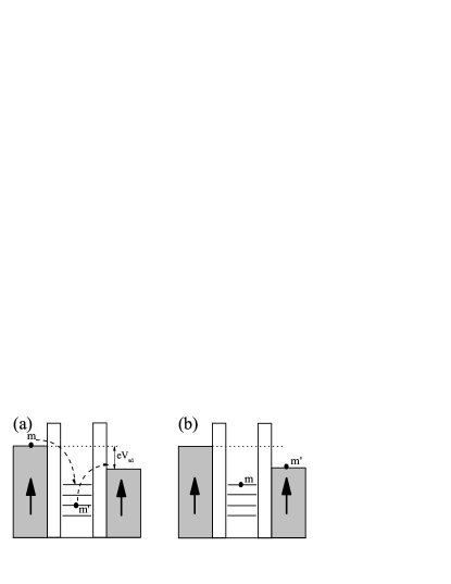
Figure 1: Schematic diagram of the cotunneling process. (a) The configuration before the tunneling and (b) the configuration after the tunneling. There are six possible tunneling processes involving different spin and orbit flips in carbon nanotube quantum dot ($m\Leftrightarrow m^{\prime}$).

Due to the presence of the spin and orbit degrees of freedom in the system studied, the Kondo resonances can originate from different cotunneling processes, as shown in Fig. 1. After some careful analysis, it is found that there are twelve possible cotunneling processes. As a result, the position of the Kondo resonance obtained from each individual process can be determined by the energy difference between the final and initial configurations, namely, $eV_{sd}=\tilde{\varepsilon}_{m^{\prime}}-\tilde{\varepsilon}_{m}$. For convenience, we mark these different contunneling processes by numbers. Explicitly, we use “1” and “4” to denote the tunnelings with both spin and orbit flip, ($|\uparrow+\rangle\leftrightarrow|\downarrow-\rangle$) and ($|\uparrow-\rangle\leftrightarrow|\downarrow+\rangle$), respectively and “2” and “5” to represent the tunnelings with only spin-flip and the orbit remains, i.e., ($|\uparrow+\rangle\leftrightarrow|\downarrow+\rangle$ ) and ($|\uparrow-\rangle\leftrightarrow|\downarrow-\rangle$), respectively and finally “3” and “6” mean ($|\uparrow+\rangle\leftrightarrow|\uparrow-\rangle$) and ($|\downarrow-\rangle\leftrightarrow|\downarrow+\rangle$), respectively, namely, the spin keeps unchanged but the orbit flips. These six cotunneling processes will lead to twelve Kondo peaks at most when all degeneracy is lifted by interactions involving spin and orbit degrees of freedom. In the following we explicitly discuss various cases. We study possible compensation effects by applying magnetic field and compare them with the results in the $SU(2)$ case. Martinek2003a ; Martinek2003b ; Pasupathy2004 ; Sindel2007 ; Hamaya2007 ; Krawiec2007 ; Lim2010 For completeness, we firstly discuss the case that the spin-orbit coupling is neglected.

III.1 Polarization effects without the spin-orbit coupling

III.1.1 Spin-polarization effect

In this case, the Kondo physics in the CNT quantum dot involves spin and orbit degrees of freedom but they are independent of each other, thus the system has the $SU(4)$ symmetry. Choi2004 There are two polarization effects to be considered, namely, spin- and orbit-polarizations. In Fig. 2 we firstly show the spin-polarization effect and its possible compensation by applying external magnetic field. When there is no any polarization in the electrodes, all energy levels in the dot are degenerate, so the Kondo resonance shows a single peak, as shown in Fig. 2 (a) for $P^{s}=0$. When the spin polarization is switched on, the Kondo peak splits into three sub-peaks, where the processes “3” and “6” are unaffected by the spin-polarization but the remaining processes are related to the spin-polarization. This is because that the former does not involve the spin flip but the other processes do involve the spin flip. Moreover, the more stronger the spin-polarization, the more larger is the distance between these three sub-peaks. Furthermore, these three sub-peaks can not be compensated by applying external magnetic field, as shown in Fig. 2 (b). This is in contrast to the statement that the spin-polarization can be compensated by applying an external magnetic field. Lim2011 On the contrary, with increasing magnetic field, these three sub-peaks split further due to orbit- and spin-Zeeman effects. It is noted that the processes “2” and “5” do not change with increasing magnetic field since in these two processes the orbital degree of freedom is not changed. Below we consider the orbit polarization effect.

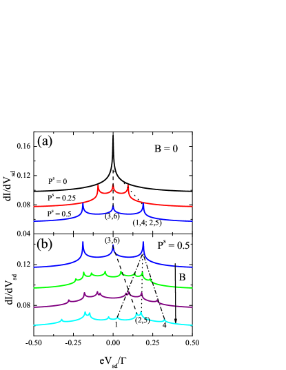
Figure 2: The spin-polarization effect and its compensation behavior in the absence of the spin-orbit coupling. (a) The Kondo peak splitting due to the spin-polarization and (b) the Kondo sub-peaks evolution under the external magnetic field applied. For clarity, here and hereafter the curves have been shifted perpendicularly to show the change of the sub-peak position with the polarization in (a) and the field in (b). The parameters used are $P^{o}=P^{k}=0$ and $\Delta_{so}=0$. In (b) the magnetic fields applied are $0,0.0025\Gamma,0.005\Gamma$ and $0.0075\Gamma$ (from top to bottom).

III.1.2 Orbit-polarization effect

When the orbit-polarization is switched on, the orbital degeneracy is removed. As a result, Fig. 3 (a) shows how the Kondo peaks split with increasing of the orbit polarization. It is observed that the processes “2” and “5” do not change with the change of the orbit polarization but the degeneracy between the processes “1” and “4” is removed. To compare Fig. 3(a) to Fig. 2 (b), the evolution of the Kondo sub-peaks under the external magnetic field without the orbit polarization is the same as that with the orbit polarization with zero field. This means that the effective exchange field induced by the orbit polarization can be completely compensated by the external magnetic field. This is true, as shown in Fig. 3 (b) (dash-dotted line). With increasing field, the processes “1” and “4” separated by the orbit polarization merge again at $B=0.006\Gamma$. This is in contrast to the spin-polarization case. The compensation effect of the orbit polarization observed here has been not reported in the literature. The physical reason of this compensation effect is that the orbit Zeeman effect dominates in such a system and the spin Zeeman is very weak. In the following we consider the case that the spin-orbit coupling is present.

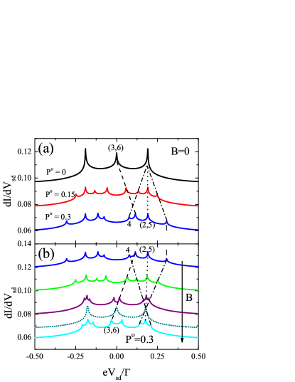
Figure 3: The orbit-polarization effect and its compensation behavior. (a) The Kondo sub-peaks splitting due to the orbit polarization and (b) the Kondo sub-peaks evolution under the external magnetic field applied. The parameters used are $P^{k}=0$ and $\Delta_{so}=0$ and $P^{s}=0.5$. In (b) the magnetic fields applied are $0,0.0025\Gamma,0.005\Gamma,0.006\Gamma,0.0075\Gamma$ (from top to bottom). The dotted line denotes the complete compensation effect at $B=0.006\Gamma$.

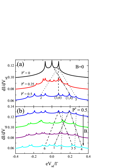
Figure 4: The spin-polarization effect and its compensation behavior in the presence of the spin-orbit coupling. (a) The Kondo peak splitting due to the spin-polarization at zero field and (b) the Kondo sub-peaks evolution under the external magnetic field applied when $P^{s}=0.5$. The parameters used are $P^{o}=P^{k}=0$ and $\Delta_{so}=0.0075\Gamma$. In (b) the magnetic fields applied are $0,0.0025\Gamma,0.005\Gamma,0.0075\Gamma$ (from top to bottom).

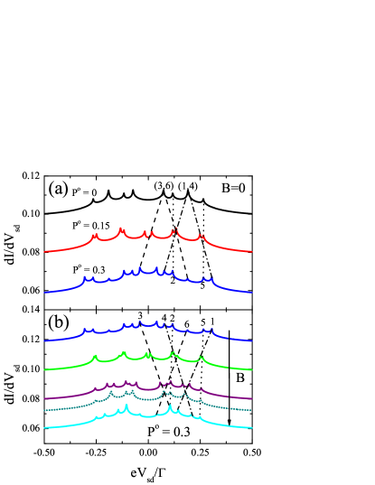
Figure 5: The orbit-polarization effect in the presence of the spin-orbit coupling and its compensation behavior. (a) The Kondo sub-peaks splitting due to the orbit polarization at zero field and (b) the Kondo sub-peaks evolution under the external magnetic fields applied when $P^{o}=0.3$. The parameters used are $P^{k}=0$ and $\Delta_{so}=0.0075\Gamma$. In (b) the magnetic fields applied are $0,0.0025\Gamma,0.005\Gamma,0.006\Gamma,0.0075\Gamma$ (from top to bottom). The dotted line denotes the compensation effect at $B=0.006\Gamma$.

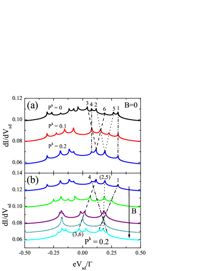
Figure 6: The Kramers polarization effect in the presence of the spin-orbit coupling and its compensation behavior. (a) The Kondo sub-peaks merging due to the Kramers polarization at zero field and (b) the Kond sub-peaks evolution under the external magnetic fields applied with $P^{k}=0.2$. The parameter used are $\Delta_{so}=0.0075\Gamma$. In (b) the magnetic fields applied are $0,0.0025\Gamma,0.005\Gamma,0.006\Gamma,0.0075\Gamma$ (from top to bottom). The dotted line denotes the compensation effect at $B=0.006\Gamma$.

III.2 Polarization effect with the spin-orbit coupling

In the presence of spin-orbit coupling, the spin- and orbit-degrees of freedom are no longer independent of each other and as a result, the SU(4) Kondo physics breaks down. Fang2008 In this case, even there is no magnetic field, the Kondo resonance shows three sub-peaks, as shown in Fig. 4(a) for $P^{s}=0$. The peak located at the center is due to the processes “1” and “4”, the side-peaks originate from the remaining processes, as pointed out in the previous work. Fang2008 This is in contrast to the single peak observed in Fig. 2(a). Below we consider the polarization effects in the electrodes. As in the last section, we firstly consider the spin-polarization effect.

III.2.1 Spin-polarization effect

With increasing the spin-polarization, the processes “3” and “6” keep unchanged, which is the same as Fig. 2 without the spin-orbit coupling. The reason is the same there. However, the remaining processes is completely different. While the degeneracy between (1,4) and (2,5) is removed by the spin-orbit coupling, the processes (1,4) keep untouched by the spin-polarization, the processes (2,5) are sensitive to the spin-polarization. This is because that in the processes (1,4) the effective field induced by the spin-polarization does not change the symmetry of the spin and orbit since the orbit flips together with the spin. This is not true for the processes (2,5) in which the orbital keeps unchanged when the spin flips. As a result, the degeneracy between the processes “2” and “5” is quickly removed with increasing the spin-polarization. Interestingly, by applying the magnetic field, the processes (2,5) keep unchanged, as shown in Fig. 4(b), the degenerates between the processes “1” and “4” and the processes “3” and “6” are removed. In this case, all degeneracy in such a system has been lifted and the Kondo resonance shows twelve sub-peak structure, as observed in Fig. 4(b). Here the magnetic field does not play a compensation role, on the contrary, it removes all possible degeneracy.

III.2.2 Orbit-polarization effect

Now we discuss the orbit-polarization effect in the presence of spin-orbit coupling. When increasing the orbit polarization, one notes that the processes “2” and “5” do not change since in these two processes the orbital degree of freedom does not flip. However, the degeneracy between the processes “1” and “4” is lifted. The processes “3” and “6” so do. As a consequence, all degeneracy in such a system is removed by the presence of spin- and orbit-polarizations. This can be seen from Fig. 5 (a), in which there are twelve sub-peaks for $P^{o}=0.3$. By applying magnetic field, one finds that the splittings of (1,4) and (3,6) observed in Fig. 5(a) can be partly removed, as shown by the dotted line in Fig. 5(b), which is roughly consistent with the curve of $P^{o}=0$ in Fig. 5(a). This is exactly the compensation effect induced by the orbit polarization.

III.2.3 Kramers-polarization effect

In the presence of the spin-orbit coupling, a novel polarization effect can be proposed, namely, the Kramers polarization. As discussed above, the presences of the spin- and orbit-polarizations can remove all degeneracy in carbon nanotube quantum dot and the Kondo resonance can show all possible twelve sub-peak structure. However, the additional Kramers polarization plays an inverse role, namely, it leads to the degeneracy in such a system, as shown in Fig. 6 (a). While the processes (1,4) are not be affected by the Kramers polarization since in such processes the spin and orbit flip together, the non-degeneracy of the processes “2” and “5” is removed when $P^{k}=0.2$. The same effect is also seen in the processes “3” and “6”. Therefore, the Kramers polarization plays an effective field to remove the non-degeneracy leaded by the spin-orbit coupling. This effective field can not be compensated by applying magnetic field, as observed in Fig. 6(b). With increasing magnetic field, the processes (2,5) keep untouched, and remaining processes are found to depend strongly on the applied magnetic field. Physically, in the processes (2,5) the orbit does not flip but in the remaining processes the orbit degree of freedom flips. The three peaks structure observed in Fig. 6(b) (the dotted line) corresponds to the spin-polarization splitting of the $SU(4)$ Kondo peak since the spin-orbit coupling is suppressed completely by the Kramers polarization and the effective field induced by the orbit polarization are compensated by the external magnetic fields. This indicates that the effective field induced by the orbital polarization can always be compensated by applying external magnetic field, which can also be seen from Fig. 6(b), in spite of the presence of the spin-orbit coupling.

IV Summary

In this paper we study the compensation effect in CNT quantum dot involving spin and orbit degrees of freedom. In comparison to the semiconductor quantum dot, the polarized electrodes attached to the dot contain three polarization effects, namely, the spin- and orbit-polarization as well as the Kramers polarization in the presence of the spin-orbit coupling. In the semiconductor quantum dot, the effective field induced by the spin-polarization can be completely compensated by applying magnetic field. However, here in the CNT quantum dot, one finds that only the effective field induced by the orbit polarization can be compensated by applying magnetic field and that induced by the spin-polarization can not be compensated. This can be due to that the orbital magnetic moment is much larger than the spin magnetic moment. This is different from the statement that the $SU(2)$ spin Kondo effects can be compensated by applying an external magnetic field. Lim2011 In addition, we also find that the effective fields induced by the spin- and orbit-polarizations remove the degeneracy but the effective field induced by the Kramers polarization can enhance the degeneracy through suppressing the spin-orbit coupling. Furthermore, the presence of the spin-orbit coupling does not change the compensation effect on the effective field on the orbit degree of freedom induced by any polarization. In such a system, the compensation effect of the effective field induced by the orbit polarization has not been reported in the literature and could be tested in the future experiments.

- (1) J. Kondo, Prog. Theor. Phys. 32, 37 (1964).
- (2) D. Goldhaber-Gordon, Hadas Shtrikman, D. Mahalu, David Abusch-Magder, U. Meirav, and M. A. Kastner, Nature (London) 391, 156 (1998).
- (3) S. M. Cronenwett, T. H. Oosterkamp, and L. P. Kouwenhoven, Science 281, 540 (1998).
- (4) J. Schmid et al., Physica (Amsterdam) 256B C258B, 182 (1998).
- (5) U. Meirav, M. A. Kastner, and S. J. Wind, Phys. Rev. Lett. 65, 771 (1990).
- (6) Y. Meir, N. S. Wingreen, and P. A. Lee, Phys. Rev. Lett. 66, 3048 (1991).
- (7) W. G. van der Wiel, S. De Franceschi, T. Fujisawa, J. M. Elzerman, S. Tarucha and L. P. Kouwenhoven, Science 289, 2105 (2000).
- (8) J. von Delft, Science 289, 2064 (2000).
- (9) D. Goldhaber-Gordon, J. Göres, M. A. Kastner, H. Shtrikman, D. Mahalu, and U. Meirav, Phys. Rev. Lett. 81, 5225 (1998).
- (10) F. Simmel, R. H. Blick, J. P. Kotthaus, W. Wegscheider, and M. Bichler, Phys. Rev. Lett. 83, 804 (1999).
- (11) S. De Franceschi, R. Hanson, W. G. van der Wiel, J. M. Elzerman, J. J. Wijpkema, T. Fujisawa, S. Tarucha, and L. P. Kouwenhoven, Phys. Rev. Lett. 89, 156801 (2002).
- (12) A. N. Pasupathy, R. C. Bialczak, J. Martinek, J. E. Grose, L. A. K. Donev, P. L. McEuen, D. C. Ralph, Science 306, 86 (2004).
- (13) K. Hamaya, M. Kitabatake, K. Shibata, M. Jung, M. Kawamura, K. Hirakawa, T. Machida, T. Taniyama, S. Ishida, and Y. Arakawa, Appl. Phys. Lett. 91, 232105 (2007).
- (14) S. Sahoo, T. Kontos, J. Furer, C. Hoffmann, M. Gräber, A. Cottet and C. Schönenberger, Nature Phys. 1, 99 (2005).
- (15) L. Hofstetter, A. Geresdi, M. Aagesen, J. Nygard, C. Schönenberger and S. Csonka, Phys. Rev. Lett. 104, 246804 (2010).
- (16) P. Zhang, Q. -K. Xue, Y. P. Wang, and X. C. Xie, Phys. Rev. Lett. 89, 286803 (2002).
- (17) N. Sergueev, Q. F. Sun, H. Guo, B. G. Wang, and J. Wang, Phys. Rev. B. 65, 165303 (2002).
- (18) J. Martinek, Y. Utsumi, H. Imamura, J. Barnas, S. Maekawa, J. Konig, and G. Schon, Phys. Rev. Lett. 91, 127203 (2003)
- (19) J. Martinek, M. Sindel, L. Borda, J. Barnas, J. Konig, G. Schon, and J. von Delft, Phys. Rev. Lett. 91, 247202 (2003)
- (20) M. Sindel, L. Borda, J. Martinek, R. Bulla, J. Konig, G. Schon, S. Maekawa, and J. von Delft, Phys. Rev. B. 76, 045321 (2007).
- (21) M. Krawiec J. Phys.: Condens. Matter 19, 346234 (2007).
- (22) J. S. Lim, M. Crisan, D. Sanchez, R. Lopez, and I. Grosu, Phys. Rev. B 81, 235309 (2010).
- (23) M. S. Choi, D. Sanchez, and R. Lopez, Phys. Rev. Lett. 92, 056601 (2004).
- (24) R. Swirkowicz, M. Wilczynski, and J. Barnas J. Phys.: Condens. Matter 18, 2291-2304 (2006).
- (25) T. Ando, J. Phys. Soc. Jpn. 69, 1757 (2000).
- (26) J. Nygard, D. Henry Cobden, and P. E. Lindelof, Nature 408, 342 (2000).
- (27) E. D. Minot, Y. Yaish, V. Sazonova, and P. L. McEuen, Nature 428, 536-539 (2004).
- (28) P. Jarillo-Herrero, J. Kong, H. S. J. van der Zant, C. Dekker, L. P. Kouwenhoven and S. D. Franceschi, Nature 434, 484 (2005); P. Jarillo-Herrero, J. Kong, H. S. J. van der Zant, C. Dekker, L. P. Kouwenhoven and S. DeFranceschi, Phys. Rev. Lett. 94, 156802 (2005).
- (29) M. S. Choi, R. Lopez, and R. Aguado, Phys. Rev. Lett. 95, 067204 (2005).
- (30) A. Makarovski, A. Zhukov, J. Liu, and G. Finkelstein, Phys. Rev. B 75, 241407 (2007).
- (31) D. Huertas-Hernando, F. Guinea, and A. Brataas, Phys. Rev. B 74, 155426 (2006).
- (32) D. V. Bulaev, B. Trauzettel, and D. Loss, Phys. Rev. B 77, 235301 (2008).
- (33) F. Kuemmeth, S. llani, D. C. Ralph, and P. L. McEuen, Nature 452, 448-452 (2008).
- (34) T.-F. Fang, W. Zuo, and H.-G. Luo, Phys. Rev. Lett. 101, 246805 (2008).
- (35) M. R. Galpin, F. W. Jayatilaka, D. E. Logan, and F. B. Anders, Phys. Rev. B 81, 075437 (2010).
- (36) J. S. Lim, R. Lopez, G. L. Giorgi, and D. Sanchez, Phys. Rev. B 83, 155325 (2011).
- (37) J. C. Le Guillou and E. Ragoucy, Phys. Rev. B 52, 2403 (1995).
- (38) J. R. Hauptmann, J. Paaske, and P. E. Lindelof, Nat. Phys. 4, 373 (2008).
- (39) D. E. Logan and M. R. Galpin, J. Chem. Phys. 130, 224503 (2009).
- (40) T.-F. Fang, W. Zuo, and H.-G. Luo, Phys. Rev. Lett. 104, 169902(E) (2010).
- (41) P. W. Anderson, Phys. Rev. 124, 41 (1961).
- (42) Y. Meir, N. S. Wingreen, and P. A. Lee, Phys. Rev. Lett. 70, 2601 (1993).
- (43) A. P. Jauho, N. S. Wingreen and Y. Meir, Rev. B 50, 5528 (1994).
- (44) D. N. Zubarev, Usp. Fiz. Nauk 71, 71 (1960) [Sov. Phys. Usp. 3, 320 (1960)].
- (45) C. Lacroix, J. Phys. F 11, 2389 (1981).
- (46) H.-G. Luo, Z.-J. Ying and S.-J. Wang, Phys. Rev. B 59, 9710 (1999).
- (47) F. D. M. Haldane, Phys. Rev. Lett. 40, 416 (1978).