Anisotropic covering of fractal sets

Abstract

We consider the optimal covering of fractal sets in a two-dimensional space using ellipses which become increasingly anisotropic as their size is reduced. If the semi-minor axis is $\epsilon$ and the semi-major axis is $\delta$, we set $\delta=\epsilon^{\alpha}$, where $0<\alpha<1$ is an exponent characterising the anisotropy of the covers. For point set fractals, in most cases we find that the number of points ${\cal N}$ which can be covered by an ellipse centred on any given point has expectation value $\langle{\cal N}\rangle\sim\epsilon^{\beta}$, where $\beta$ is a generalised dimension. We investigate the function $\beta(\alpha)$ numerically for various sets, showing that it may be different for sets which have the same fractal dimension.

1 Introduction

Figures 1 and 2 illustrate two different fractal point sets in two dimensions (their origins will be described shortly). The fractal dimensions (as defined in [1, 2]) of these sets are very similar (the correlation dimension are $D_{2}\approx 1.76$ and $D_{2}\approx 1.71$ respectively), but inspection of these figures suggests that the fine-scale structure of these sets is quite different. In this paper we consider whether it is possible to make a distinction between the local structures of fractals by using covering sets which become increasingly anisotropic as the covers are made smaller. We show that this can distinguish different sets which have the same fractal dimension. Moreover, we shall argue that the use of anisotropic covers can be important in analysing the scattering of radiation from fractal distributions of matter.

The sets illustrated in figures 1 and 2 are point set fractals which arise as models for the distribution of particles resulting from two distinct physical processes. Figure 1 illustrates a model of particles in a turbulent flow, in circumstances where inertial effects are large enough to ensure that the particles are not simply advected. It is known that such systems may exhibit clustering [3] and that the attractor is a fractal measure [4, 5]. An enlargement of a subset of figure 1 shows that the particle distribution is locally highly anisotropic, with the particles tending to be clustered close to lines in the plane, even though the statistics of the distribution are globally rotationally invariant. This is consistent with the structure of strange attractors in low-dimensional dissipative dynamical systems, where the attractor has a local structure which is the Cartesian product of a line and a one-dimensional Cantor set [6]. The second example, figure 2, is a diffusion-limited aggregation (DLA) cluster in two dimensions [7]. The local structure of this set cannot be approximated as a Cartesian product. Also, if a subset of a DLA cluster such as figure 2 is examined at a higher magnification, it does not appear to be more markedly anisotropic in structure. Thus it appears as if some fractal sets, such as that illustrated in figure 1, may exhibit a pronounced anisotropy under magnification, whereas this effect is much less pronounced (or possibly absent) in others, such as figure 2.

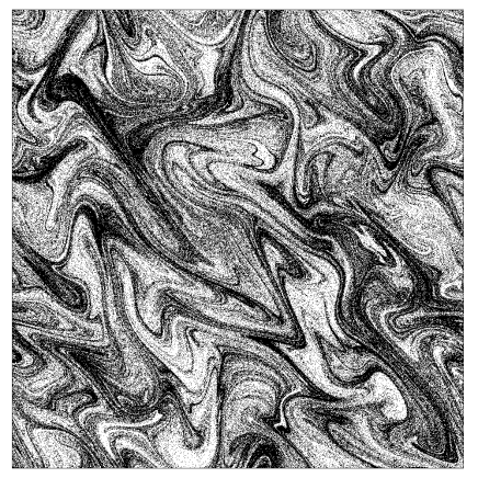
Figure 1: Distribution of particles with significant inertia moving in a two-dimensional area-preserving velocity field (the equations of motion are specified in section 3). The particles tend to cluster and for the parameters used in this simulation (see section 3) the correlation dimension is $D_{2}\approx 1.76$

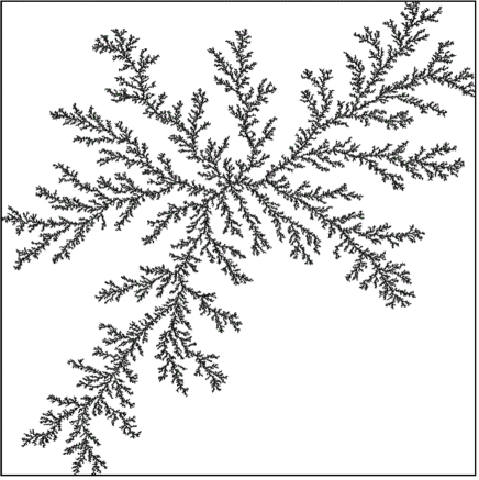
Figure 2: Distribution of particles determined by a diffusion-limited aggregation (DLA) process. This distribution has (approximately) the same fractal dimension as figure 1: $D_{2}\approx 1.71$

Throughout this paper we confine our attention to point sets in the plane, but generalisations to higher dimensions are obvious. We use the following approach to characterise the local structure of a point set. Take a given element of the set, and consider an ellipse centred on this point, with its semi-minor axis of length $\epsilon$ and its semi-major axis of length $\delta=\epsilon^{\alpha}$, where $0<\alpha<1$. We assume $\delta\ll\xi$ and $\epsilon\ll\xi$, where $\xi$ is the characteristic lengthscale of the system below which fractal scaling is observable, and that $\epsilon\gg\epsilon_{0}$, where $\epsilon_{0}$ is the lengthscale where the fractal scaling is cut off by the finite number of points sampling the fractal measure. We then choose the orientation of the cover so that it maximises the number of other points which are contained in this ellipse. We denote the number of points under this optimally-oriented cover by ${\cal N}$. We repeat this for ellipses centred on other randomly selected points in the set, and compute the average value $\langle{\cal N}\rangle$ of the number of points which can be covered. In most of the examples of point-set fractals which we investigated, the mean number of points in this ellipse is found to have a power-law dependence:

$$\langle{\cal N}(\epsilon,\alpha)\rangle\sim\epsilon^{\beta(\alpha)}\ ,\ \ \ \ \delta=\epsilon^{\alpha}$$ (1)

where the exponent $\beta$ depends upon $\alpha$. In the case where $\alpha=1$, the ellipse is a circle, so that this case reduces to a definition of the correlation dimension: $D_{2}=\beta(1)$ (compare with the discussion of the correlation dimension in [8]). In general $\beta$ must decrease monotonically as $\alpha$ decreases.

A related approach to the characterisation of fractal sets was proposed by Grassberger and co-workers [8, 9, 10, 11], who considered covering a set (which is embedded in a $d$-dimensional space) with $d$-dimensional ellipsoids, with principal axes $\epsilon_{i}$, ordered so that $\epsilon_{1}>\epsilon_{2}>\ldots>\epsilon_{d}$. Their work emphasises the case where the local structure of the fractal is a Cartesian product of sets, with dimensions $\Delta_{i}$, ordered so that $\Delta_{1}>\Delta_{2}>\ldots>\Delta_{d}$. It is asserted that the ellipsoids cover most efficiently when they align with the principal axes, such that the longest axes align with the directions of the highest density sets. According to this hypothesis the number of points covered is expected to satisfy

$$\langle{\cal N}\rangle\sim\epsilon_{1}^{\Delta_{1}}\epsilon_{2}^{\Delta_{2}}\epsilon_{3}^{\Delta 3}\ldots\epsilon_{d}^{\Delta_{d}}\ .$$ (2)

Examining the dependence of ${\cal N}$ upon the $\epsilon_{i}$ would allow the partial dimensions $\Delta_{i}$ to be determined. This approach was mentioned in several papers [8, 9, 10, 11], with the motivation to characterise a fractal set by means of its partial dimensions, $\Delta_{i}$, satisfying $\sum_{i=1}^{d}\Delta_{i}=D_{2}$. These works do not prescribe how (or whether) the ratio $\epsilon_{i+1}/\epsilon_{i}$ approaches zero as $\epsilon_{1}\to 0$. In our work this limiting behaviour is specified by the parameter $\alpha$. Our numerical investigations encompass fractal sets which have a Cartesian product structure, and those which do not.

In the case of point set fractals which represent a physical distribution of particles, the existence of a highly anisotropic local structure has important physical implications for the scattering of light. It is known that s-wave scattering of light from a fractal point set gives rise to an algebraic relation between the scattering wavenumber $k$ and the scattered intensity $I$, such that

$$I(k)\sim k^{-D_{2}}\ .$$ (3)

Heuristic arguments supporting this are developed in [12]; see [13] for a discussion of some of the complications which can arise in verifying this suggestion. The distribution of this scattering intensity may, however, be highly inhomogeneous. In particular, if the particles have a strong tendency to accumulate along lines in two dimensions (like the example shown in figure 1), or on planes in higher dimensions, light may scatter specularly from these structures. We argue that this motivates the investigation of the anisotropic covering with ellipsoids. Consider weak scattering of light with wavelength $\epsilon$ which propagates as a beam of width $\delta$. When the path length for light scattered from different particles is large compared to $\epsilon$, the scattering of light from ${\cal N}$ particles is incoherent, so that the contribution to the scattered intensity is $I\sim{\cal N}$. If, however, an ellipsoid of major axis $\delta$ and minor axis $\epsilon$ can be aligned to cover ${\cal N}$ particles, then there will exist directions where the path length difference is less than one wavelength, so that this set of ${\cal N}$ particles scatters light coherently (see figure 3). In these directions where the condition for specular reflection is satisfied by the optimal covering ellipsoid, there is a greatly increased intensity $I\sim{\cal N}^{2}$.

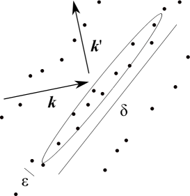
Figure 3: Scattering of a beam of light with wavevector $k$, width $\delta$ and wavelength $\epsilon$: a cluster of ${\cal N}$ particles covered by an $\epsilon$-$\delta$ ellipse scatters light coherently when the condition for specular reflection is satisfied. The wavevector $\mbox{\boldmath$k$}^{\prime}$ satisfies the condition for specular reflection if the major axis of the ellipse is perpendicular to $\mbox{\boldmath$k$}-\mbox{\boldmath$k$}^{\prime}$. In this case the scattered intensity from the particles under the cover is increased by a factor of order ${\cal N}$.

We have argued that light scattering from fractal sets may be extremely inhomogeneous because of specular scattering from particles which accumulate on surfaces. This motivated us to study the covering of a fractal by anisotropic covering sets, and the results are reported here. We investigate the dependence of the generalised dimension $\beta$ upon the anisotropy exponent $\alpha$. We show that the form of the function $\beta(\alpha)$ can distinguish between different fractal sets which have the same value of the correlation dimension $D_{2}=\beta(1)$. The description of light scattering proved to be a very complex issue, which will be considered elsewhere.

2 Some elementary estimates

Before discussing our numerical investigations, we consider some simple arguments about the form of the generalised dimension $\beta(\alpha)$, defined by equation (1).

First we address the issue of whether the exponent $\beta$ exists. When $\alpha=1$, the exponent $\beta$ coincides with the correlation dimension of the set. For other values of $\alpha$, we do not know of any general argument which proves that the dependence of the optimal covering ${\cal N}$ has a power law relation to the size $\epsilon$ of the covering elements. For most of the point-set fractals which we examined we did find good numerical evidence that $\langle{\cal N}\rangle\sim\epsilon^{\beta}$ for small values of $\epsilon$ (extending down towards values of $\epsilon$ where the discrete sampling of the set becomes a limitation). The exceptions occurred for some cases of the motion of inertial particles in a random flow, and for some of the sets considered in section 4, including the example illustrated in figure 4: these are discussed in sections 3 and 4 respectively.

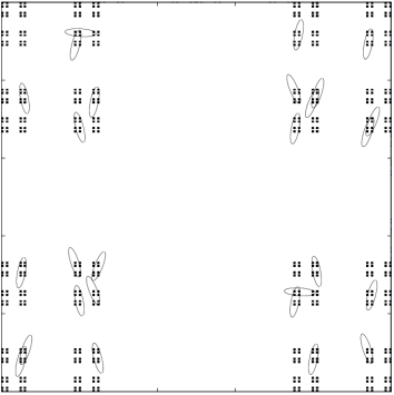
Figure 4: In the case where the fractal set is a Cartesian product of two Cantor sets, with dimensions $D_{x}$ and $D_{y}$ in the $x$ and $y$ directions, the optimal covering ellipse might be expected to have its major axis aligned with the direction corresponding to the denser set. In the case $D_{y}>D_{x}$, the major axis of the ellipse would be expected to align with the $y$-axis (vertical in this figure). Here we illustrate a sample of the actual optimal covers, which have a distribution of angles of their principal axes.

Next we give an upper bound on $\beta(\alpha)$. Let us consider the expectation $\langle{\cal N}\rangle$ for the case where ${\cal N}$ is independent of the orientation of the ellipse. The total number of particles in a disc of radius $\delta$ is proportional to $\delta^{D_{2}}$. If the set is locally isotropic then the coverage is independent of the angle of the major axis of the ellipse, and a fraction $\epsilon/\delta$ of these points lie in the ellipse. Recalling that $\delta=\epsilon^{\alpha}$, for this isotropic fractal we have $\langle{\cal N}\rangle\sim\delta^{D_{2}-1}\epsilon\sim\epsilon^{1-\alpha+\alpha D_{2}}\equiv\epsilon^{\beta_{+}(\alpha)}$, so that

$$\beta_{+}(\alpha)=1+(D_{2}-1)\alpha\ .$$ (4)

is an upper bound on the exponent $\beta$.

We were not able to obtain a precise and non-trivial lower bound for $\beta(\alpha)$, but the following argument suggests a possible form for a lower bound. Consider the case where the point fractal samples a Cartesian product of two one-dimensional Cantor sets, with dimensions $D_{x}$ and $D_{y}$. In the following we assume that $D_{y}\geq D_{x}$. Because the set is ‘denser’ in the direction of the $y$-axis, we expect that the optimal alignment of each ellipse is when its major axis is aligned with the $y$-axis (the same hypothesis was proposed in [8, 9]). The expected number of particles captured by a covering ellipse is then $\langle{\cal N}\rangle\sim\delta^{D_{y}}\epsilon^{D_{x}}=\epsilon^{\alpha D_{y}+D_{x}}$, so that the dimension of this product set is

$$\beta(\alpha)=\alpha D_{y}+D_{x}\ .$$ (5)

Now consider the smallest possible dimension which could be achieved according to this argument, if we allow the dimensions $D_{x}$, $D_{y}$ of the component sets to vary so that $D_{x}+D_{y}=D_{2}$. The greatest number of particles in the ellipse, and hence the smallest dimension, is obtained by setting $D_{y}=1$ and $D_{x}=D_{2}-1$. This gives a putative lower bound to the dimension:

$$\beta_{-}(\alpha)=D_{2}-1+\alpha\ .$$ (6)

The assumption that the covering ellipses align precisely with the $y$-axis is not really correct, as evidenced by figure 4. It is plausible that the probability for an ellipses to be significantly mis-aligned decreases as $\epsilon\to 0$, but we were not able to obtain conclusive numerical evidence. We note that the argument leading to the proposed lower bound, $\beta_{-}(\alpha)$, is very similar to that presented in [8, 9] to motivate the concept of partial dimensions.

In addition to the fact that the optimal covering ellipses do not align perfectly with the preferred axes, there is a further complication which could affect the argument leading to the estimate in equation (6). In sets such as that illustrated in figure 1, the local structure is a Cartesian product of a line and a one-dimensional Cantor set. The line is, however, curved. It is interesting to consider whether this curvature can alter the estimate in equation (6). In order to consider the effect of this curvature, introduce two coordinates: $y$ is a coordinate for the expanding (unstable) manifold centred on the reference particle and $x$ is a coordinate for the stable manifold. Because the manifolds are curved, the equation of the unstable manifold will be of the form $x\sim Cy^{2}$ for small $y$, where $C$ is a constant. Consider a family of ellipses, with fixed $\delta$ and decreasing $\alpha$ which are aligned so as to provide the optimal cover for a cluster centred on a reference particle. As $\alpha$ is reduced, the curvature of the unstable manifold can become important, because it will take a cluster of particles outside the covering ellipse (see figure 5). This happens when $x(\delta)\sim\epsilon$, that is when $C\epsilon^{2\alpha}\sim\epsilon$. Accordingly, we might propose that the optimal covering strategy of aligning the principal axis of the ellipses with the unstable manifold starts to break down when at a critical value of the exponent, $\alpha_{\rm c}=\frac{1}{2}$. On the basis of this argument we would expect that $\beta(\alpha)$ might exceed equation (6) when $\alpha<\frac{1}{2}$, in cases where the fractal is generated by a dynamical system for which the lines representing the unstable manifold are curved.

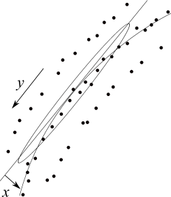
Figure 5: In many dynamical systems the attractor is locally a Cartesian product of a Cantor set and a line. If this line is curved, an ellipse may cease to be an efficient cover as $\alpha$ is decreased. The $x$- and $y$-coordinates are referred to in section 2.

3 Numerical investigations of dynamical fractals

Figure 1 illustrates the distribution of independently moving inertial particles in a random velocity field. The equations of motion for the position of a given particle are [3]

$$\dot{\mbox{\boldmath$r$}}=\mbox{\boldmath$v$}\ ,\ \ \ \dot{\mbox{\boldmath$v$}}=-\gamma[\mbox{\boldmath$v$}-\mbox{\boldmath$u$}(\mbox{\boldmath$r$}(t),t)]$$ (7)

where $\gamma$ is the rate at which the particles relax towards the fluid velocity, and where $\mbox{\boldmath$u$}(\mbox{\boldmath$r$},t)$ is a randomly fluctuating velocity field satisfying the incompressibility condition $\mbox{\boldmath$\nabla$}\cdot\mbox{\boldmath$u$}=0$. Particles in the fluid flow cluster if the damping timescale $\gamma^{-1}$ is comparable to a timescale characterising the velocity field. In the simulations used in this paper, we used a random vector field with a very small correlation time, using the same definitions as in [14], where the importance of inertial effects is characterised by a dimensionless parameter, which was referred to as $\varepsilon$ in that work, but which is denoted by $\eta$ in this paper. It is defined in terms of the correlation function of the velocity gradient experienced by a particle with trajectory $\mbox{\boldmath$r$}(t)$:

$$\eta^{2}=\frac{1}{2\gamma}\int_{-\infty}^{\infty}{\rm d}t\ \left\langle\left(\frac{\partial u_{x}}{\partial x}\right)(\mbox{\boldmath$r$}(t),t)\left(\frac{\partial u_{x}}{\partial x}\right)({\bf 0},0)\right\rangle\ .$$ (8)

In figure 1, we showed a realisation of the long-time dynamics. The velocity is periodic on the unit square, and was generated from a random stream function $\psi(\mbox{\boldmath$r$},t)$. The statistics of the stream function are $\langle\psi(\mbox{\boldmath$r$},t)\rangle=0$, $\langle\psi(\mbox{\boldmath$r$},t)\psi({\bf 0},0)\rangle=A^{2}\exp(-|\mbox{\boldmath$r$}|^{2}/2\xi^{2})\exp(-|t|/\tau)$, with $\xi=0.1$, $\tau$ small and $A$ chosen such that $\eta=0.1$. The correlation dimension for this value of $\eta$ is $D_{2}\approx 1.76$ [14].

We examined whether the mean value of the optimal covering number, $\langle{\cal N}\rangle$, shows a power-law dependence upon $\epsilon$. The data for $\eta=0.1$, shown in figure 6, are a good fit to a power-law for values of $\alpha$ as low as $0.2$. At very small values of $\alpha$, the area of the ellipses decreases very rapidly as $\epsilon\to 0$, so that the values of $\langle{\cal N}\rangle$ become too small to give reliable results.

Figure 6: The mean number of points in an optimal cover, $\langle{\cal N}\rangle$, as a function of $\epsilon$, for various values of $\alpha$. The slope increases monotonically with $\alpha$, which ranges from $\alpha=0.2$ to $\alpha=1$ in increments of $0.2$. These data, for the random flow model with $\eta=0.1$, show excellent fits to a power law over a wide range of $\epsilon$.

For the inertial particles model we found a number of cases where the covering data was not well fitted by a power-law in $\epsilon$. This occurs for small values of $\alpha$ and for values of $\eta$ where the value of $D_{2}$ is close to its minimum, which is $D_{2}\approx 1.35$ at $\eta\approx 0.35$. Figure 7 illustrates the case where the fit to a power-law was the least good.

Figure 7: Same as figure 6, except $\eta=0.4$, where $D_{2}\approx 1.36$. In this case the covering data are not a good fit to a power-law in $\epsilon$ for $\alpha\leq 0.75$.

In figure 8 we exhibit the $\beta(\alpha)$ curves for this systems at several different values of the inertial parameter $\eta$. Fractal attractors of dynamical systems typically have a local structure which is a Cartesian product of a Cantor set and a line. Following the discussion in section 2 we therefore expect that the exponent $\beta(\alpha)$ should be given by equation (6), that is $\beta(\alpha)\approx\beta_{-}(\alpha)$. We find, however, that $\beta_{-}(\alpha)$ is not a very good approximation, and figure 8 shows that different $\beta(\alpha)$ curves may be obtained for cases with the same fractal dimension (these arise because $D_{2}$ has a minimum with respect to varying $\eta$) . In section 2 we also suggested that the generalised dimension $\beta(\alpha)$ might be higher than $\beta_{-}(\alpha)$ when $\alpha\leq\frac{1}{2}$ because the unstable manifold is curved. Figure 8 does not show evidence of any discontinuous change at $\alpha=\frac{1}{2}$.

Figure 8: $\beta(\alpha)$ for inertial particles in a random velocity field, using a model defined in [14]. The curves are labelled according to the parameter $\eta$ which quantifies the importance of particle inertia.

We also investigated $\beta(\alpha)$ for fractals generated by two other dynamical processes. We simulated diffusion limited aggregation (DLA, one realisation of which was illustrated in figure 2), in the usual manner [7]: points make a random walk on a lattice until they contact the cluster, after which they are frozen and become part of the growing set. In the case of isotropic diffusion, the correlation dimension of the resulting cluster is $D_{2}\approx 1.71$. The values of the slopes $\beta$ extracted from least-squares fits similar to those in figure 6 are plotted in figure 9 as a function of $\alpha$.

We also investigated the fractal generated by the Sinai map, defined by

$$x_{n+1} = x_{n}+y_{n}+a\cos(2\pi y_{n}){\rm mod}\,1$$

$$y_{n+1} = x_{n}+2y_{n}{\rm mod}\,1$$ (9)

with $a=0.35$, which has an attractor with correlation dimension $D_{2}\approx 1.62$. The $\beta(\alpha)$ curve for this map is also shown in figure 9.

Figure 9: $\beta(\alpha)$ for a diffusion limited aggregation (DLA) cluster with $2.7\times 10^{5}$ particles, and for the Sinai map with $a=0.35$.

4 Sierpinski substitution fractals

The examples of dynamical fractals which we considered in section 3 are all multifractal sets, and it is desirable to investigate $\beta(\alpha)$ for a model which is a simple fractal, avoiding the complications that arise when dealing with multifractal sets [15]. Here we construct a class of generalisations of the Sierpinski carpet, which are simple fractals rather than multifractal measures. The construction that we use is closely related to one proposed independently by Bedford [16] and McMullen [17]. We show that different elements from this class of sets can have different $\beta(\alpha)$ functions despite having precisely the same value of $D_{2}=\beta(1)$.

We generate an approximation to a fractal set by a hierarchical process consisting of $n$ generations. We generate a set of $M^{n}$ points, where $M$ is an integer, as follows. The points $\mbox{\boldmath$x$}_{k}$ lie in the unit square $[0,1]\otimes[0,1]$, and have coordinates of the form $(x_{i},y_{i})=(i/N_{1}^{n},j/N_{2}^{n})$, where $N_{1}$, $N_{2}$ are positive integers satisfying $N_{1}N_{2}>M$.

We define a ‘masking matrix’ ${\bf F}$ with elements $F_{ij}$ as an $N_{1}\times N_{2}$ matrix which has elements which are either $1$ or $0$, and we let $M$ be the number of non-zero elements of ${\bf F}$. We construct the model set by the following recursive construction. Consider the ‘first generation’ set of $M$ points $\mbox{\boldmath$x$}_{k}$, labelled by an index $=1\ldots M$, where a point is placed at $((i-1)/N_{1},(j-1)/N_{2})$ if $F_{ij}=1$. At the next generation each of these points is replaced by a set of $M$ points, based on a lattice with spacings $N_{1}^{-2}$ and $N_{2}^{-2}$ in the $x$ and $y$ directions respectively, which are selected by the criterion that $F_{ij}=1$. In general, after $n$ generations each point $\mbox{\boldmath$x$}_{k}$ is replaced by $M$ points with positions $\mbox{\boldmath$x$}_{k^{\prime}}$, where $k^{\prime}$ is an index of the $(N_{1}N_{2})^{n+1}$ points, with positions

$$\mbox{\boldmath$x$}^{\prime}_{k^{\prime}}=\mbox{\boldmath$x$}_{k}+\left(\frac{i-1}{N_{1}^{n+1}},\frac{j-1}{N_{2}^{n+1}}\right)\ .$$ (10)

A point labelled by $(i,j)$ added to the set if and only if $F_{ij}=1$.

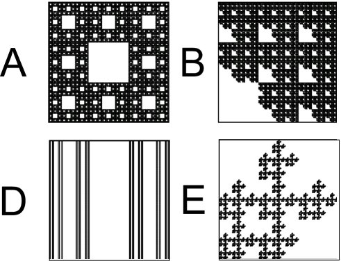
Figure 10: Examples of fractal sets generated by the construction defined in section 4. In all of these examples, $N_{1}=N_{2}=3$. The Cantor set is then defined by listing the zero elements of the masking matrix (the labels correspond to the cases considered in figure 11): (A) $F_{22}=0$, $D={\rm ln}\,8/{\rm ln}\,3$, (B) $F_{11}=0$, $D={\rm ln}\,8/{\rm ln}\,3$, (D) $F_{21}=F_{22}=F_{23}=0$, $D={\rm ln}\,6/{\rm ln}\,3$, (E) $F_{13}=F_{31}=F_{33}=0$, $D={\rm ln}\,6/{\rm ln}\,3$ .

As an example, consider the case where $N_{1}=N_{2}=3$ and where $F_{22}=0$ is the only element of ${\bf F}$ which is equal to zero, so that $M=8$. Iterating this construction gives a version of the Sirepinski carpet set, illustrated in figure 10A, with dimension $D={\rm ln}\,8/{\rm ln}\,3$. By varying the zero elements of the masking matrix, we can generate many other Cantor sets, some examples of which are illustrated in the other panels of figure 10. The resulting sets are clearly simple fractals (as opposed to multifractals). By making other choices of the masking matrix we can construct other Cantor sets with dimension

$$D=\frac{2\,{\rm ln}\,M}{{\rm ln}\,(N_{1}\,N_{2})}\ .$$ (11)

This construction allows us to create distinct fractal sets with exactly the same dimension, such as in panels A and B or panels D and E of figure 10. Moreover, by a suitable choice of the masking matrix, we can generate fractal sets which are Cartesian products (such as figure 10D), as well as those which are not (such as figures 10A, B, E).

We investigated the function $\beta(\alpha)$ for sets which are produced by this generalised Sierpinski construction. The results are illustrated in figure 11, for seventeen sets produced using a $3\times 3$ masking matrix. The key at the right hand side of the figure indicates the pattern of deletions in the masking matrix, ordered by the number of deleted points.

First we discuss those sets which are a Cartesian product. These include examples D, I, L, P and Q in figure 11. The simplest example is set D in figures 10 and 11. For this set, equation (6) predicts that $\beta(\alpha)=D-1+\alpha$, which shows excellent agreement with figure 11. By setting $N_{1}=N_{2}=3$ and $F_{12}=F_{21}=F_{23}=F_{32}=F_{22}=0$ we produce a set with dimension $D={\rm ln}\,4/{\rm ln}\,3=2\,{\rm ln}\,2/{\rm ln}\,3$, which is a Cartesian product of two Cantor sets of dimension $D_{x}=D_{y}=D/2={\rm ln}\,2/{\rm ln}\,3$. This is example I in figure 11. Example L is closely related: this set is similar to example I, rotated by $\pi/4$. These data show quite poor agreement with the prediction from equation (5), from which we expect $\beta(\alpha)=D(1+\alpha)/2$ (but good agreement with each other). The other two examples in figure 11 which are Cartesian products are very simple: P is a Cartesian product of a line and a point, and Q is the product of a Cantor set of dimension ${\rm ln}\,2/{\rm ln}\,3$ and a point. For these examples there is excellent agreement with the predictions of equations (6) and (5), which indicate straight lines of slope unity and ${\rm ln}\,2/{\rm ln}\,3$ respectively.

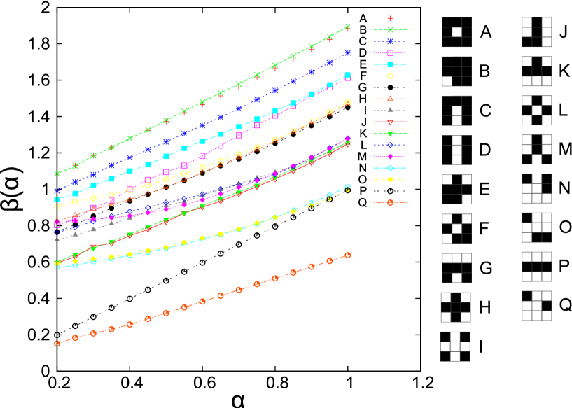
Figure 11: $\beta(\alpha)$ for the generalised Sierpinski model. The curves are labelled by a key giving the zero elements of the masking matrix in white.

Figure 11 also shows $\beta(\alpha)$ in cases where the set is not a Cartesian product. These differ from the data for the Cartesian product sets. They can be organised into sets which have apparently identical $\beta(\alpha)$ curves. In most of the cases examined in figure 11, sets which have the same value of $M$ (and hence of $D_{2}$) have $\beta(\alpha)$ curves which are identical, to within numerical fluctuations. Examples of such groups are $(M=8:{\rm A,B})$, $(M=5:{\rm G},{\rm F})$, $(M=4:{\rm J},{\rm K})$, $(M=3:{\rm N},{\rm O})$. Note, however, that for $M=4$, set M is not a Cartesian product and yet has a $\beta(\alpha)$ curve which is clearly different from sets J and K.

We noted that examples I and L in figure 11, which are Cartesian products of two one-dimensional Cantor sets, had $\beta(\alpha)$ functions which show quite poor agreement with the expected result, equation (5). It appears possible that this anomaly might arise because these sets are a degenerate case, where $D_{x}=D_{y}$. We therefore also considered two examples which are a Cartesian product of two Cantor sets with different dimensions, namely $N_{1}=4$, $N_{2}=3$, with non-zero elements $F_{11}=F_{13}=F_{41}=F_{43}=1$ (which is the set illustrated in figure 4), and $N_{1}=5$, $N_{2}=3$, with non-zero elements $F_{11}=F_{13}=F_{51}=F_{53}$. These are Cartesian products of two one-dimensional Cantor sets with dimensions $D_{x}=\frac{1}{2}$ ($4\times 3$ case) or $D_{x}={\rm ln}\,2/{\rm ln}\,5$ ($5\times 3$ case), and $D_{y}={\rm ln}\,2/{\rm ln}\,3$. In figure 12 we show the dependence of $\langle{\cal N}\rangle$ upon $\epsilon$ on a double-logarithmic scale, for the set illustrated in figure 4. For each value of $\alpha$, including $\alpha=1$, the plots appear to have an oscillation about a straight line, which makes it difficult to determine accurate values for $\beta(\alpha)$. In figure 13 we show our best estimates for $\beta(\alpha)$ for these three fractal sets, compared with the theoretical prediction in the $4\times 3$ case, given by equation (5). There are substantial deviations from the theoretical curve, but note that these are no larger than the errors in determining the fractal dimension $D_{2}=\beta(1)$ for these sets. We conclude that although the agreement with (5) is poor, this is due to difficulties in fitting the data, and there is no persuasive evidence that (5) is incorrect.

Figure 12: For the set illustrated in figure 4, it is difficult to fit the exponent $\beta(\alpha)$ because of an oscillation in the dependence of ${\rm ln}\,\langle{\cal N}\rangle$ upon ${\rm ln}\,\epsilon$.

Figure 13: $\beta(\alpha)$ for three cases of the generalised Sierpinski model which are Cartesian products of Cantor sets, based upon $3\times 3$, $4\times 3$ and $5\times 3$ deletion matrices.

Section 2 concluded with an argument which suggests that when the set is locally a Cartesian product of a line and a Cantor set, the function $\beta(\alpha)$ may have a different behaviour when $\alpha<\frac{1}{2}$ if the lines are curved. The data on the clustering of inertial particles (reported in section 3) were not a good fit to equation (6), and they did not show a clear signature that $\alpha=\frac{1}{2}$ is a critical point. A more controlled test was made with the Sierpinski fractals considered in this section. The sets were modified by applying a shift to all of the $y$-coordinates:

$$\mbox{\boldmath$x$}=(x,y)\rightarrow\mbox{\boldmath$x$}^{\prime}=(x^{\prime},y^{\prime})=(x,y+C\sin(2\pi x))\ .$$ (12)

The sets which are reported upon in figure 11 were deformed according to this rule, with $C=\frac{1}{2}$. The $\beta(\alpha)$ exponents remained unchanged for all of these sets (within numerical fluctuations comparable to those in figure 11).

5 Concluding remarks

This paper has reported the first systematic study of fractals using a set of covers which become more anisotropic as they are made smaller. The growth of the anisotropy is described by a parameter $\alpha$, and we characterised the efficiency of covering by a generalised dimension $\beta(\alpha)$. We found that different sets with the same correlation dimension $D_{2}$ can have different $\beta(\alpha)$, as was demonstrated very clearly for the simple Sierpinski substitution fractals which we considered in section 4.

In the case where the fractal is locally a Cartesian product of a line and a Cantor set, a heuristic argument (similar to that given in [8] and subsequent papers) suggest that $\beta(\alpha)$ should be given by (6). We find that this expression works well for simple model sets of the type considered in section 4, and for the Sinai map, where the attractor is locally a Cartesian product of a line and a Cantor set. In the case of clustering of inertial particles, however, we find that equation (6) does not give a good approximation to $\beta(\alpha)$. In cases where the Cantor set does not have a Cartesian product structure, we were not able to derive an expression for $\beta(\alpha)$, and we find persuasive evidence that this function is non-universal.

In three or more dimensions there may also be a tendency for particles to accumulate on filamentary structures, as well as on planes. This could be characterised by defining the exponent $\beta$ as a function of two parameters, $\alpha_{1}$, $\alpha_{2}$ defining a covering ellipsoid with principal axes $\epsilon$, $\epsilon^{\alpha_{1}}$ and $\epsilon^{\alpha_{2}}$.

This study was partly motivated by the desire to understand the inhomogeneity of light scattering from fractal distributions of particles, but our investigations indicate that this is a very complex problem, which will be considered in a separate publication.

Acknowledgements. HRK thanks the Open University for a postgraduate studentship.

References

References

- [1] B. B. Mandelbrot, The Fractals Geometry of Nature, Freeman, San Fancisco, (1982).
- [2] K. Falconer, Fractal Geometry: mathematical foundations and applications, Wiley, New York, (1990).
- [3] M. R. Maxey, J. Fluid Mech., 174, 441, (1987).
- [4] J. Sommerer and E. Ott, Science, 359, 334, (1993).
- [5] M. Wilkinson, B. Mehlig, S. Östlund and K. P. Duncan, Phys. Fluids, 19, 113303, (2007).
- [6] E. Ott, Chaos in Dynamical Systems, 2nd edition, Cambridge: University Press, (2002).
- [7] T. A. Witten Jr and L. M. Sander, Phys. Rev. Lett., 47, 1400, (1981).
- [8] P. Grassberger and I. Procaccia, Physica D, 13, 34-54, (1984).
- [9] P. Grassberger, Phys. Lett., A107, 101-5, (1985).
- [10] A. Politi, R. Badii and P. Grassberger, J. Phys. A: Math. Gen., 21, L763-9, (1988).
- [11] P. Grassberger, R. Badii, A. Politi, J. Stat. Phys., 51, 135-78, (1988).
- [12] S. K. Sinha, Physica D, 38, 310, (1989).
- [13] C. P. Dettman, N. E. Frankel, T. Taucher, Phys. Rev. E, 49, 3171-78, (1993).
- [14] M. Wilkinson, B. Mehlig and K. Gustavsson, Europhys. Lett., 89, 50002, (2010).
- [15] T. C. Halsey, M. H. Jensen, L. P. Kadanoff, I. Procaccia and B. I. Shraiman, Phys. Rev. A, 33, 1141, (1986).
- [16] T. Bedford, Ph.D. thesis, University of Warwick, (1984).
- [17] C. McMullen, Nagoya Math. J., 96, 9, (1984).