Second-kind integral solvers for TE and TM problems of diffraction by open arcs

Abstract

We present a novel approach for the numerical solution of problems of diffraction by open arcs in two dimensional space. Our methodology relies on composition of weighted versions of the classical integral operators associated with the Dirichlet and Neumann problems (TE and TM polarizations, respectively) together with a generalization to the open-arc case of the well known closed-surface Calderón formulae. When used in conjunction with spectrally accurate discretization rules and Krylov-subspace linear algebra solvers such as GMRES, the new second-kind TE and TM formulations for open arcs produce results of high accuracy in small numbers of iterations—for low and high frequencies alike.

1 Introduction

Problems of diffraction by infinitely thin open surfaces play central roles in a wide range of problems in science and engineering, with important applications to antenna and radar design, electronics, optics, etc. Like other wave scattering problems, open surface problems can be treated by means of numerical methods that rely on approximation of Maxwell’s Equations over volumetric domains (on the basis of, e.g., finite-difference or finite-element methods) as well as methods based on boundary integral equations. As a result of the singular character of the electromagnetic fields in the vicinity of open edges, open-surface scattering configurations present major difficulties for both volumetric and boundary integral methods. Boundary integral approaches, which require discretization of domains of lower dimensionality than those involved in volumetric methods, can generally be treated efficiently, even for high-frequencies, by means of accelerated iterative scattering solvers [3, 6, 24]. Unfortunately, integral methods for open surfaces do not give rise, at least in their classical formulations, to Fredholm integral operators of the second-kind, and can therefore prove to be computationally expensive—as the eigenvalues of the resulting equations accumulate at zero and/or infinity and, thus, iterative solution of these equations often requires large numbers of iterations.

This paper presents new Fredholm integral equations of second-kind and associated numerical algorithms for problems of scattering by two-dimensional open arcs $\Gamma$ (i.e., infinite cylinders of cross-section $\Gamma$) under either transverse electric (TE) or transverse magnetic (TM) incident fields. The new second-kind Fredholm equations (which result from composition of appropriately modified versions $\mathbf{S}_{\omega}$ and $\mathbf{N}_{\omega}$ of the classical single-layer and hypersingular integral operators $\mathbf{S}$ and $\mathbf{N}$) provide, for the first time, a generalization of the classical closed-surface Calderón formulas to the open-arc case. In particular, the new formulations possess highly favorable spectral properties: their eigenvalues are highly clustered, and they remain bounded away from zero and infinity, even for problems of very high frequency. When used in conjunction with spectrally accurate discretization rules and Krylov-subspace linear algebra solvers such as GMRES, the new open-arc formulations produce results of high accuracy in small numbers of iterations—for low and high frequencies alike.

The new second-kind formulation for the TM problem is particularly beneficial, as it gives rise to order-of-magnitude improvements in computing times over the corresponding weighted hypersingular formulation. Such gains do not occur in the TE case: although the new second-kind TE equation requires fewer iterations than the corresponding weighted first kind formulation, the total computational cost of the second-kind equation is generally higher in the TE case—since the application of the first-kind operator can be significantly less expensive than the application of the composite second-kind operator.

The difficulties that arise as integral equations are used to treat open surface scattering problems are of course well known, and many contributions have been devoted to their treatment. Like the present work, references [22] and [8] seek to tackle these problems by means of generalizations of the classical Calderón relations to the case of open surfaces. The first of these contributions establishes that the combination $\mathbf{N}\mathbf{S}$ can be expressed in the form $\mathbf{I}+\mathbf{T}_{K}$, where the kernel $\mathbf{K}(x,y)$ of the operator $\mathbf{T}_{K}$ has local singularity of at most $O\left(\frac{1}{|x-y|}\right)$. This early result however does not take into account the singular edge behavior; the resulting operator $\mathbf{T}_{K}$ is not compact (in fact it gives rise to extreme singularities at the edge [16]) and $\mathbf{I}+\mathbf{T}_{K}$ is therefore not a second-kind operator in any numerically meaningful functional space. When used in conjunction with boundary elements that vanish on the edges (by means of well-chosen projections) however, the combination $\mathbf{N}\mathbf{S}$ does give rise to reduction of iteration numbers, as demonstrated in reference [8] through numerical examples for low frequency problems. This contribution does not include details on accuracy, and it does not utilize integral weights to resolve the solution’s edge singularity. A related but different method was introduced in [1] which exhibits, once again, low iteration numbers for low-frequency problems, but which does not resolve the singular edge behavior and for which no accuracy studies have been presented. Finally, high-order integration rules for the single-layer and hypersingular operators adapted to open arcs were introduced in a Galerkin framework in [29, 12, 28]. These methods have thus far only been applied for simple geometries and at low frequencies, and limited information is available on the actual convergence properties and performance of their computational implementations.

A second class of methods include those proposed in references [2, 20, 13]. The contribution [2], some aspects of which are incorporated in our method, treats the Dirichlet problem for Laplace’s equation by means of second kind equations. The basis of this approach lies in the observation that the cosine basis has the dual positive effect of diagonalizing the logarithmic potential for a straight arc and removing the singular edge behavior—so that the inverse of the logarithmic potential can be easily computed and used as a preconditioner to produce a second kind operator for a general arc. The approach [20], which also uses a cosine basis, treats the Neumann problem for the non-zero frequency Helmholtz equation with spectral accuracy by means of first kind equations. The contribution [13], finally, treats, just like [2], the Laplace problem by means of second-kind equations resulting from inversion of the straight arc logarithmic potential; like [20], further, it produces spectral accuracy through use of the cosine transforms. The second-kind integral approach developed in [2] and later revisited in [13] seems essentially limited to the specific problem for which it was proposed: neither an extension to the Neumann problem nor to the full three dimensional problem seem straightforward. And, more importantly, this approach does not lead to adequately preconditioned equations for non-zero frequencies: a simple experiment conducted in Section 3.4 shows that a direct generalization of the algorithm [2] to the Helmholtz problem generally requires significantly more linear algebra iterations than are necessary if the operator $\mathbf{S}_{\omega}$ alone is used.

The remainder of this paper is organized as follows: after recalling in Section 2 the classical boundary integral formulations for the TE and TM open-arc scattering problems, in Sections 3.1 and 3.2 we present our new weighted operators $\mathbf{S}_{\omega}$ and $\mathbf{N}_{\omega}$ as well as certain periodized counterparts $\tilde{S}$ and $\tilde{N}$ (which are obtained by considering a sinusoidal changes of variables for source and observation points). Our main result, the generalized Calderón formula, is presented in Section 3.3. Section 3.4 then presents results of numerical evaluation of eigenvalues for a non-trivial open arc problem, illustrating the spectral properties of previous open-arc operators as well as the second kind operators introduced in this paper. Theoretical considerations concerning the new second-kind equations are presented in Section 4, including a succinct but complete proof of the open-arc Calderón formulae; a more detailed theoretical discussion, including full mathematical technicalities, can be found in [16]. The high-order quadrature rules we use for evaluation of the new integral operators are described in Section 5. Numerical results, finally, are presented in Section 6 for a wide range of frequencies and for various geometries (including a brief study of resonant open cavities) demonstrating the uniformly well conditioned character of the integral formulations proposed in this paper.

2 Preliminaries

Let $\Gamma$ denote a smooth open arc in the plane. The TE and TM problems of scattering by the open arc $\Gamma$ amount to two-dimensional problems for the Helmholtz equation with Dirichlet and Neumann boundary conditions on $\Gamma$, respectively:

$$\left\{\begin{array}[]{llll}\Delta u+k^{2}u=0\quad\mbox{outside}\quad\Gamma,&u|_{\Gamma}=f&\mbox{(TE)}\\ \Delta v+k^{2}v=0\quad\mbox{outside}\quad\Gamma,&\frac{\partial v}{\partial\textbf{n}}|_{\Gamma}=g&\mbox{(TM)}.\end{array}\right.$$ (1)

Here n denotes the normal to $\Gamma$, and $f$ and $g$ are given in terms of the incident electric excitation $u^{inc}$: $f=-u^{inc}$ and $g=-\partial u^{inc}/\partial\textbf{n}$ on $\Gamma$.

2.1 Classical open-arc equations for TE and TM problems

The (unique) solutions $u$ and $v$ of the TE and TM problems above can be expressed, for $\mathbf{r}\not\in\Gamma$, in terms of single- and double-layer potentials of the form $u(\mathbf{r})=\int_{\Gamma}G_{k}(\mathbf{r},\mathbf{r}^{\prime})\mu(\mathbf{r}^{\prime})d\ell^{\prime}$ and $v(\mathbf{r})=\int_{\Gamma}\frac{\partial G_{k}(\mathbf{r},\mathbf{r}^{\prime})}{\partial\textbf{n}_{\mathbf{r}^{\prime}}}\nu(\mathbf{r}^{\prime})d\ell^{\prime}$; see e.g. [29, 30, 26]. Here $\textbf{n}_{\mathbf{r}^{\prime}}$ is a unit vector normal to $\Gamma$ at the point $\mathbf{r}^{\prime}\in\Gamma$ (we assume, as we may, that $\textbf{n}_{\mathbf{r}^{\prime}}$ is a smooth function of $\mathbf{r}^{\prime}\in\Gamma$), and, calling $H_{0}^{1}$ the first Hankel function of order zero,

$$G_{k}(\mathbf{r},\mathbf{r}^{\prime})=\left\{\begin{array}[]{ll}\frac{i}{4}H_{0}^{1}(k|\mathbf{r}-\mathbf{r}^{\prime}|),&k>0\\ -\frac{1}{2\pi}\ln|\mathbf{r}-\mathbf{r}^{\prime}|,&k=0\end{array}\right.$$ (2)

and $\frac{\partial G_{k}(\mathbf{r},\mathbf{r}^{\prime})}{\partial\mathbf{n}_{\mathbf{r}^{\prime}}}=\mathbf{n}_{\mathbf{r}^{\prime}}\cdot\nabla_{\mathbf{r}^{\prime}}G_{k}(\mathbf{r},\mathbf{r}^{\prime}).$ Denoting by $\mathbf{S}$ and $\mathbf{N}$ the single-layer and hypersingular operators

$$\mathbf{S}[\mu](\mathbf{r})=\int_{\Gamma}G_{k}(\mathbf{r},\mathbf{r}^{\prime})\mu(\mathbf{r}^{\prime})d\ell^{\prime}\quad,\quad\mathbf{r}\in\Gamma,$$ (3)

and

$$\begin{split}\mathbf{N}[\nu](\mathbf{r})=&\;\frac{\partial}{\partial\textbf{n}_{\mathbf{r}}}\int_{\Gamma}\frac{\partial G_{k}(\mathbf{r},\mathbf{r}^{\prime})}{\partial\textbf{n}_{\mathbf{r}^{\prime}}}\nu(\mathbf{r}^{\prime})d\ell^{\prime}\\ \stackrel{{\scriptstyle\mathrm{def}}}{{=}}&\lim\limits_{z\rightarrow 0^{+}}\frac{\partial}{\partial z}\int_{\Gamma}\frac{\partial G_{k}(\mathbf{r}+z\mathbf{n}_{\mathbf{r}},\mathbf{r}^{\prime})}{\partial\textbf{n}_{\mathbf{r}^{\prime}}}\nu(\mathbf{r}^{\prime})d\ell^{\prime}\quad,\quad\mathbf{r}\in\Gamma,\end{split}$$ (4)

further, the densities $\mu$ and $\nu$ are the unique solutions of the integral equations

$$\mathbf{S}[\mu]=f,\quad\mathbf{N}[\nu]=g.$$ (5)

It is known that the eigenvalues of the integral operators in Equations (5) accumulate at zero and infinity, respectively (see e.g. Figure 1). As a result (and as illustrated in Section 6), solution of these equations by means of Krylov-subspace iterative solvers such as GMRES generally require large numbers of iterations. In addition, as discussed in Section 2.3, the solutions $\mu$ and $\nu$ of equations (5) are not smooth at the end-points of $\Gamma$, and, thus, they give rise to low order convergence (and require high discretization of the densities for a given accuracy) if standard quadrature methods are used. Details in these regards are provided in what follows.

2.2 Calderón relation for closed and open arcs.

As is well known [9, 21, 10] second-kind formulations for closed surfaces (arcs) result from: (1) The classical jump relations associated with singular integral operators, as well as (2) application of the Calderón formula

$$\mathbf{N}_{c}\mathbf{S}_{c}=-\frac{\mathbf{I}}{4}+\mathbf{K}_{c},$$ (6)

which shows that the composition of the closed-surface hypersingular and single-layer operators $\mathbf{N}_{c}$ and $\mathbf{S}_{c}$ equals a compact perturbation $\mathbf{K}_{c}$ of the identity.

In the open-surface context however, jump relations cannot be exploited since, according to the boundary conditions (1), the same limits must be reached on both sides of the open surface $\Gamma$. Further, use of the combined operator $\mathbf{N}\mathbf{S}$ does not lead to well-posed equations: as shown in [16], the image under $\mathbf{N}\mathbf{S}$ of the constant function $1$ is highly singular, with edge asymptotics $\mathbf{NS}[1](\mathbf{r})=O\left(\frac{1}{d(\mathbf{r})}\right)$, $\mathbf{r}\in\Gamma$, where $d(\mathbf{r})$ denotes the Euclidian distance to the edge. The combination $\mathbf{N}\mathbf{S}$ is also problematic in the functional framework set forth in [29, 30, 27], since the image under $\mathbf{S}$ of the Sobolev space $H^{\frac{1}{2}}(\Gamma)$ (as defined in [27]) is larger than the domain of definition of $\tilde{H}^{\frac{1}{2}}(\Gamma)$ (as defined in [27]) of the operator $\mathbf{N}$.

2.3 Regularity and singular behavior at the edge

The singular character of the solutions of equations (5) is well documented [27, 17]: $\mu$ and $\nu$ can be expressed in the forms

$$\mu\sim\frac{\chi_{1}}{\sqrt{d}}+\eta,\quad\nu\sim\chi_{2}\sqrt{d}+\zeta,$$ (7)

where $d$ denotes the distance to the edge, $\chi_{1}$ and $\chi_{2}$ are smooth cut-off functions, and where the functions $\eta$ and $\zeta$ are somewhat smoother than $\mu$ and $\nu$. More recently furthermore, it was established [17] that expressions such as (7) can be viewed as part of an expansion in powers of $d^{1/2}$ which can be carried out as long as the degree of smoothness of the surface and the right hand side of the equations allow it. For example, if the curve itself and the functions $f$ and $g$ in (5) are infinitely differentiable, it follows that

$$\mu=\frac{\alpha}{\sqrt{d}},\quad\nu=\beta\sqrt{d},$$ (8)

where $\alpha$ and $\beta$ are infinitely differentiable functions throughout $\Gamma$, up to and including the endpoints [17]. Thus the singular character of these solutions is fully characterized by the factors $d^{1/2}$ and $d^{-1/2}$ in equation (8).

3 Well-posed Second-Kind Integral Equation Formulations

3.1 Weighted operators

In view of the regularity results (8), we introduce a positive integral weight $\omega(\mathbf{r})>0$ with asymptotic edge behavior $\omega\sim d^{1/2}$ at the edge (by which it is implied that the quotient $\omega/d^{1/2}$ is infinitely differentiable up to the edge), and we define the weighted operators

$$\mathbf{S}_{\omega}[\alpha]=\mathbf{S}\left[\frac{\alpha}{\omega}\right],\quad\mathbf{N}_{\omega}[\beta]=\mathbf{N}[\omega\beta],$$ (9)

so that, in view of the discussion of Section 2.3, for smooth functions $f$ and $g$, the solutions of the equations

$$\mathbf{S}_{\omega}[\alpha]=f\quad\mbox{and}\quad\mathbf{N}_{\omega}[\beta]=g$$ (10)

are also smooth.

Without loss of generality, we choose a smooth parameterization $\mathbf{r}(t)=\left(x(t),y(t)\right)$ of $\Gamma$ defined in the interval $[-1,1]$, and we define the weight $\omega$ canonically as $\omega(\mathbf{r}(t))=\sqrt{1-t^{2}}.$ As a result, the operators $\mathbf{S}_{\omega}$ and $\mathbf{N}_{\omega}$ give rise to the parameter-space operators

$$S_{\omega}[\varphi](t)=\int_{-1}^{1}G_{k}\left(\mathbf{r}(t),\mathbf{r}(t^{\prime})\right)\frac{\varphi(t^{\prime})}{\sqrt{1-t^{\prime 2}}}\;\tau(t^{\prime})dt^{\prime},$$ (11)

and

$$\begin{split}N_{\omega}[\psi](t)=\lim\limits_{z\rightarrow 0^{+}}\frac{\partial}{\partial z}\int_{-1}^{1}\frac{\partial}{\partial\textbf{n}_{\mathbf{r}(t^{\prime})}}G_{k}\left(\mathbf{r}(t)+z\textbf{n}_{\mathbf{r}(t)},\mathbf{r}(t^{\prime})\right)\\ \psi(t^{\prime})\tau(t^{\prime})\sqrt{1-t^{\prime 2}}dt^{\prime},\end{split}$$ (12)

defined on functions $\varphi$ and $\psi$ of the variable $t$, $-1\leq t\leq 1$; in these equations we have set $\tau(t)=|\frac{d\textbf{r}(t)}{dt}|$. Clearly, for $\varphi(t)=\alpha(\mathbf{r}(t))$ and $\psi(t)=\beta(\mathbf{r}(t))$ we have $\mathbf{S}_{\omega}[\alpha](\mathbf{r}(t))=S_{\omega}[\varphi](t)$ and $\mathbf{N}_{\omega}[\beta](\mathbf{r}(t))=N_{\omega}[\psi](t).$

3.2 Periodized spaces and regularity

Introducing the changes of variables $t=\cos\theta$ and $t^{\prime}=\cos\theta^{\prime}$, and defining $\textbf{n}_{\theta}=\textbf{n}_{\mathbf{r}(\cos\theta)}$, we obtain the periodic weighted single-layer and hypersingular operators

$$\tilde{S}[\gamma](\theta)=\int_{0}^{\pi}G_{k}(\mathbf{r}(\cos\theta),\mathbf{r}(\cos\theta^{\prime}))\gamma(\theta^{\prime})\tau(\cos\theta^{\prime})d\theta^{\prime}$$ (13)

and

$$\tilde{N}[\gamma](\theta)=\lim\limits_{z\rightarrow 0^{+}}\frac{\partial}{\partial z}\int_{0}^{\pi}\frac{\partial}{\partial\textbf{n}_{\theta^{\prime}}}G_{k}(\mathbf{r}(\cos\theta)+z\textbf{n}_{\theta},\mathbf{r}(\cos\theta^{\prime}))\\ \gamma(\theta^{\prime})\tau(\cos\theta^{\prime})\sin^{2}\theta^{\prime}d\theta^{\prime}.$$

Clearly then, the solutions to the periodic equations

$$\tilde{S}[\tilde{\varphi}]=\tilde{f},\quad\tilde{N}[\tilde{\psi}]=\tilde{g},$$ (14)

where $\tilde{f}(\theta)=f(\mathbf{r}(\cos\theta))$ and $\tilde{g}(\theta)=g(\mathbf{r}(\cos\theta))$, are related to the solutions of equations (10) by the relations

$$\tilde{\varphi}(\theta)=\varphi(\cos\theta)\quad,\quad\tilde{\psi}(\theta)=\psi(\cos\theta).$$ (15)

In view of (15), the solutions to equations (14) are smooth and periodic, and it is therefore natural to study the properties of $\tilde{S}$ and $\tilde{N}$ in the the Sobolev spaces $H^{s}_{e}(2\pi)$ of $2\pi$ periodic and even functions cf. [31, 5].

Definition 1.

Let $s\in\mathbb{R}$. The Sobolev space $H^{s}_{e}(2\pi)$ is defined as the set of $2\pi$-periodic functions of the form $v(\theta)=\frac{1}{2}a_{0}+\sum\limits_{m=1}^{\infty}a_{m}\cos(m\theta)$ for which the $s$-norm $\|v\|_{s}^{2}=|a_{0}|^{2}+2\sum\limits_{m=1}^{\infty}m^{2s}|a_{m}|^{2}$ is finite.

Clearly the set $\{\cos(n\theta):n\in\mathbb{N}\}$ is a basis of the Hilbert space $H^{s}_{e}(2\pi)$ for all $s$.

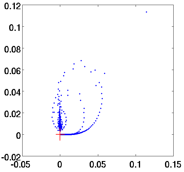
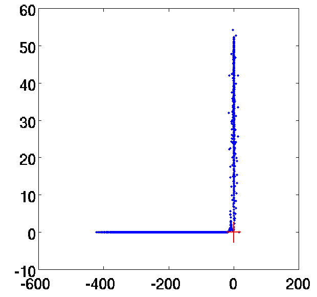
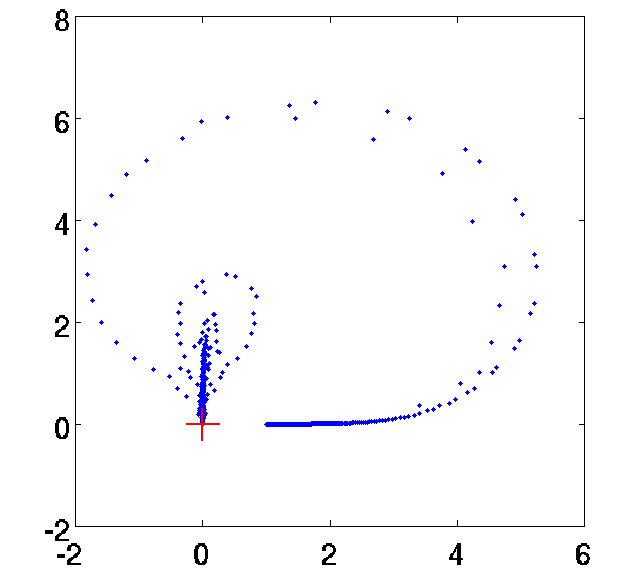
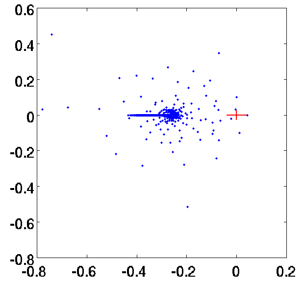
Figure 1: Eigenvalue distribution for the spiral-shaped arc displayed in Figure 3, with frequency $\frac{L}{\lambda}=100$, for the various operators under consideration. Left $\tilde{S}$. Left-center $\tilde{N}$. Right-center $\tilde{S}_{0}^{-1}\tilde{S}$. Right $\tilde{N}\tilde{S}$. Note the important difference of scale between the four plots.

3.3 Generalized Calderón Formula

Given the smoothness of the solutions of the equations arising from the weighted periodic operators $~{}\tilde{S}$ and $~{}\tilde{N}$, and in light of equation (6), it is reasonable to consider the composition $\tilde{N}\tilde{S}$ as possible basis for solution of open-arc problems. As stated in the following theorem and demonstrated below, this combination does indeed give rise to a second-kind integral formulation. The statement of the theorem makes use of the concept of bicontinuity: an operator $L$ between two Hilbert spaces is said to be bicontinuous if and only if $L$ is invertible and both $L$ and $L^{-1}$ are continuous operators.

Theorem 1.

• For all $s>0$ the operators $\tilde{N}$ and $\tilde{S}$ define bicontinuous mappings $\tilde{S}:H^{s}_{e}(2\pi)\rightarrow H^{s+1}_{e}(2\pi)$ and $\tilde{N}:H^{s+1}_{e}(2\pi)\rightarrow H^{s}_{e}(2\pi)$. Thus, the composite operator $\tilde{N}\tilde{S}$ is bicontinuous from $H^{s}_{e}(2\pi)$ into $H^{s}_{e}(2\pi)$ for all $s>0$.

• The generalized Calderón formula

  $$\tilde{N}\tilde{S}=\tilde{J}^{\tau}_{0}+\tilde{K}$$ (16)

  holds, where ${\tilde{K}}:H^{s}_{e}(2\pi)\rightarrow H^{s}_{e}(2\pi)$ is a compact operator, and where $\tilde{J}^{\tau}_{0}:H^{s}_{e}(2\pi)\rightarrow H^{s}_{e}(2\pi)$ is a bicontinuous operator independent of the frequency $k$.

• The set $\sigma_{s}$ of eigenvalues of $\tilde{J}^{\tau}_{0}:H^{s}_{e}(2\pi)\to H^{s}_{e}(2\pi)$ equals the union of the discrete set $\Lambda_{\infty}=\{\lambda_{0}=-\frac{\ln 2}{4},\quad\lambda_{n}=-\frac{1}{4}-\frac{1}{4n}:n>0\}$ and a certain open set $\Lambda_{s}$ which is bounded away from zero and infinity. The sets $\Lambda_{s}$ are nested, they form a decreasing sequence, ($\Lambda_{s}\varsubsetneq\Lambda_{s^{\prime}},s>s^{\prime}$) and they satisfy $\bigcap_{s>0}\bar{\Lambda}_{s}=\{-\frac{1}{4}\}$, where $\bar{\Lambda}_{s}$ denotes the closure of $\Lambda_{s}$.

It follows that the open-arc TE and TM scattering problems (1) can be solved by means of the second-kind integral equations

$$\tilde{N}\tilde{S}[\tilde{\varphi}]=\tilde{N}[\tilde{f}]\quad\mbox{and}$$ (17)

$$\tilde{N}\tilde{S}[\tilde{\psi}]=\tilde{g},$$ (18)

respectively. The smooth and periodic solutions $\tilde{\varphi}$ and $\tilde{\psi}$ of these equations are related to the singular solutions $\mu$ and $\nu$ of equations (5) via $\mu\left(\mathbf{r}(\cos\theta)\right)=\tilde{\varphi}(\theta)/\sin\theta$ and $\nu\left(\mathbf{r}(\cos\theta)\right)=\sin\theta\left(\tilde{S}[\tilde{\psi}](\theta)\right).$ We thus see that, through introduction of the weight $\omega$ and use of spaces of even and $2\pi$-periodic functions, a picture emerges for the open-surface case that resembles closely the one found for closed-surface configurations: the generalized Calderón relation (16) is analogous to the Calderón formula (6), and mapping properties in terms of the complete range of Sobolev spaces are recovered for $\tilde{S}$ and $\tilde{N}$, in a close analogy to the framework presented in [14, 21] for the operators $\mathbf{N}_{c}$ and $\mathbf{S}_{c}$.

3.4 Eigenvalue Distributions

In order to gain additional insights on the character of the various $k\neq 0$ open-arc operators under consideration (namely, $\tilde{S}$, $\tilde{N}$, $\tilde{N}\tilde{S}$ as well as a generalization to non-zero frequencies of the operator introduced in reference [2]), we consider their corresponding eigenvalue distributions. In Figure 1 we thus display the eigenvalues associated with these operators, for the spiral-shaped arc displayed in Figure 3 and described in Section 6, as they were produced by means of the quadrature rules presented in Section 5 and subsequent evaluation of matrix eigenvalues. The frequency was chosen to ensure a size to wavelength ratio $\frac{L}{\lambda}=100$, where $L$ is the length of the arc and $\lambda$ the wavelength of the incident wave. As expected, the eigenvalues of $\tilde{S}$ tend slowly to zero, the eigenvalues of $\tilde{N}$ are large, while the eigenvalues of $\tilde{N}\tilde{S}$ are bounded away from zero and infinity, and they accumulate at $-\frac{1}{4}$.

The $k>0$ generalization of the equation [2], whose operator eigenvalues are displayed in the center-right portion of Figure 1, is obtained from right-multiplication of the single layer operator in equation (10) by the inverse of the flat-arc zero-frequency single-layer operator $\tilde{S}_{0}^{\tau}$ (defined in equation (39) below); the resulting equation is given by

$$\tilde{S}(\tilde{S}_{0}^{\tau})^{-1}[\tilde{\varphi}]=\tilde{f}.$$ (19)

This equation, which can be re-expressed in the form $\left(I+(\tilde{S}-\tilde{S}_{0}^{\tau})(\tilde{S}_{0}^{\tau})^{-1}\right)[\tilde{\varphi}]=\tilde{f}$, is a second-kind Fredholm integral equation: the operator $\left(\tilde{S}-\tilde{S}_{0}^{\tau}\right)(\tilde{S}_{0}^{\tau})^{-1}:H^{s}_{e}(2\pi)\rightarrow H^{s}_{e}(2\pi)$ is compact. Unfortunately, the spectrum of the operator in equation (19) is highly unfavorable at high frequencies, as illustrated in the center-right image in Figure 1. Such poor spectral distributions translate into dramatic increases, demonstrated in Table 6, in the number of iterations required to solve (19) by means of Krylov subspace solvers as the frequency grows. In fact, a direct comparison with Table 3 shows that the second-kind integral equation (19) may require many more iterations at non-zero frequencies than the original first-kind equation (14).

4 Theoretical Considerations

This section presents a proof of Theorem 1. The argument proceeds by consideration of the flat-arc zero-frequency case (Sections 4.1 through 4.3) and subsequent extension to the general case (Sections 4.4,4.5 and 4.6). A more detailed discussion, including full mathematical technicalities, can be found in [16].

4.1 Flat arc at zero-frequency

In the particular case where the frequency vanishes ($k=0$) and the curve under consideration is the flat strip ($\Gamma=[-1,1]$), the operator $\tilde{S}$ reduces to Symm’s operator

$$\tilde{S}_{0}[\tilde{\varphi}](\theta)=-\frac{1}{2\pi}\int_{0}^{\pi}\ln|\cos\theta-\cos\theta^{\prime}|\tilde{\varphi}(\theta^{\prime})d\theta^{\prime},$$ (20)

whose well-known diagonal property [31, 5] in the cosine basis $e_{n}(\theta)=\cos n\theta$,

$$\tilde{S_{0}}[e_{n}]=\lambda_{n}e_{n},\textbf{ }\lambda_{n}=\left\{\begin{array}[]{cc}\frac{\ln 2}{2}&n=0\\ \frac{1}{2n},&n\geq 1\end{array}\right.$$ (21)

plays a central role in our analysis. Note that, in particular, equation (21) establishes the bicontinuity of the operator $\tilde{S}_{0}$ from $H^{s}_{e}(2\pi)$ into $H^{s+1}_{e}(2\pi)$. The corresponding property of bicontinuity (from $H^{s+1}_{e}(2\pi)$ into $H^{s}_{e}(2\pi)$) for the weighted flat-strip, zero-frequency hypersingular operator

$$\tilde{N}_{0}[\tilde{\psi}](\theta)=\frac{1}{2\pi}\lim\limits_{z\rightarrow 0}\int_{0}^{\pi}\frac{\partial^{2}}{\partial z^{2}}\left(\ln\sqrt{(\cos\theta-\cos\theta^{\prime})^{2}+z^{2}}\right)\tilde{\psi}(\theta^{\prime})\sin^{2}\theta^{\prime}d\theta^{\prime}$$

results, in turn, from our study of the operator $\tilde{J}_{0}$ in Section 4.2.

An integration by parts argument presented in reference [20] gives rise to the factorization $\tilde{N}_{0}=\tilde{D}_{0}\tilde{S}_{0}\tilde{T}_{0}$ where

$$\tilde{D}_{0}[\tilde{\varphi}](\theta)=\frac{1}{\sin\theta}\frac{d\tilde{\varphi}(\theta)}{d\theta}$$ (22)

and

$$\tilde{T}_{0}[\tilde{\varphi}](\theta)=\frac{d}{d\theta}\left(\tilde{\varphi}(\theta)\sin\theta\right).$$ (23)

As a result, for the flat-arc at zero-frequency case, the composite operator $\tilde{N}\tilde{S}$, is given by

$$\begin{split}\tilde{J}_{0}=\tilde{N}_{0}\tilde{S}_{0}=\tilde{D}_{0}\tilde{S}_{0}\tilde{T}_{0}\tilde{S}_{0}.\end{split}$$ (24)

4.2 The operator $\tilde{J}_{0}$

It is easy to evaluate the action of the operator $\tilde{J}_{0}$ on the cosine basis: in view of equation (24), using (21) and expressing $\tilde{T}_{0}[e_{n}]$ as a linear combination of cosines (which results from simple trigonometric manipulations) we obtain the relation

$$\tilde{J}_{0}[e_{n}](\theta)=\left\{\begin{array}[]{ll}-\frac{\ln 2}{4}&n=0\\ -\cos\theta\frac{\sin n\theta}{4n\sin\theta}-\frac{\cos n\theta}{4},&n\geq 1.\end{array}\right.$$ (25)

Clearly then,

$$\tilde{J}_{0}[\tilde{\varphi}](\theta)=-\frac{\tilde{\varphi}(\theta)}{4}-\frac{\cos\theta}{4}\tilde{C}[\tilde{\varphi}](\theta)+\frac{1-\ln 2}{4\pi}\int_{0}^{\pi}\tilde{\varphi}(u)du,$$ (26)

where the operator $\tilde{C}$ is defined by

$$\tilde{C}[e_{n}](\theta)=\left\{\begin{array}[]{ll}0&n=0\\ \frac{\sin n\theta}{n\sin\theta},&n\geq 1.\end{array}\right.$$ (27)

The right hand side of equation (26) may appear to bear a direct connection with the classical closed-curve Calderón formula (6). Yet, unlike the operator $\mathbf{K}_{c}$ in equation (6), the operator $\tilde{C}$ is not compact–see Section 4.3. It is easy, however, to verify that $\tilde{C}$ can also be expressed in the form

$$\tilde{C}[\tilde{\varphi}](\theta)=\frac{\theta(\pi-\theta)}{\pi\sin\theta}\left[\frac{1}{\theta}\int_{0}^{\theta}\tilde{\varphi}(u)du-\frac{1}{\pi-\theta}\int_{\theta}^{\pi}\tilde{\varphi}(u)du\right],$$ (28)

and is therefore closely related to the Césaro operator $\mathcal{C}[\eta](x)=\frac{1}{x}\int_{0}^{x}\eta(u)du.$ Since $\mathcal{C}$ is bounded (but not compact) from $L^{2}[0,b]$ into $L^{2}[0,b]$ [4] (where $L^{2}[0,b]$ denotes the space of square-integrable functions in the interval $[0,b]$), it follows that $\tilde{C}:\quad H^{s}_{e}(2\pi)\rightarrow H^{s}_{e}(2\pi)$ is a continuous operator for all $s>0$, and, therefore, $\tilde{J}_{0}:H^{s}_{e}(2\pi)\rightarrow H^{s}_{e}(2\pi)$ is also a continuous operator.

Composing the operator $\tilde{I}_{0}=-4\tilde{S}_{0}^{-1}\tilde{C}\tilde{S}_{0}\tilde{T}_{0}$ with $\tilde{J}_{0}$ from the right on one hand, and from the left, on the other, and applying the two resulting composite operators to the basis $e_{n}$, shows that $\tilde{I}_{0}$ is the inverse of $\tilde{J}_{0}$, and that $\tilde{I}_{0}$ is a continuous operator from $H^{s}_{e}(2\pi)$ into $H^{s}_{e}(2\pi)$. It follows that $\tilde{J}_{0}$ is a bicontinuous operator. As indicated in Section 4.1, finally, the bicontinuity of $\tilde{N}_{0}$ from $H^{s+1}_{e}(2\pi)$ into $H^{s}_{e}(2\pi)$ follows directly from equation (24) and the corresponding bicontinuity properties of $\tilde{S}_{0}$ and $\tilde{J}_{0}$.

4.3 Eigenvalues of $\tilde{J}_{0}$

Re-expressing (25) in the form

$$\tilde{J}_{0}[e_{n}](\theta)=\left\{\begin{array}[]{ll}-\frac{\ln 2}{4}&n=0\\ -\frac{\sin(n+1)\theta}{4n\sin\theta}+\frac{\cos n\theta}{4n}-\frac{\cos n\theta}{4},&n>0,\end{array}\right.$$ (29)

and making use the well-known expansion [11, 19]

$$\frac{\sin(n+1)\theta}{\sin\theta}=\left\{\begin{array}[]{ll}\sum\limits_{k=0}^{p}(2-\delta_{0k})\cos 2k\theta,&n=2p\\ 2\sum\limits_{k=0}^{p}\cos(2k+1)\theta,&n=2p+1,\end{array}\right.$$ (30)

we obtain

$$\begin{split}\tilde{J}_{0}[e_{n}]=\left\{\begin{array}[]{ll}\lambda_{n}e_{n}-\frac{1}{2n}\sum\limits_{k=0}^{p-1}(1-\frac{\delta_{0k}}{2})e_{2k},&n=2p,\;p\geq 0\\ \lambda_{n}e_{n}-\frac{1}{2n}\sum\limits_{k=0}^{p-1}e_{2k+1},&n=2p+1,\;p\geq 0\\ \end{array}\right.,\end{split}$$ (31)

where the diagonal elements $\lambda_{n}$ are given by

$$\lambda_{n}=\left\{\begin{array}[]{lr}-\frac{\ln 2}{4},&n=0\\ -\frac{1}{4}-\frac{1}{4n},&\quad n>0.\end{array}\right.$$ (32)

In view of (29), the operator $\tilde{J}_{0}$ can be viewed as an infinite upper-triangular matrix. The diagonal terms $\lambda_{n}$ of this matrix are eigenvalues of $\tilde{J}_{0}$; the corresponding eigenvectors $v_{n}$, in turn, can be expressed in terms of a finite linear combination of the first $n$ cosine basis functions: $v_{n}=\sum_{k=0}^{n}c_{k}^{n}e_{k}$. This establishes that the set $\Lambda_{\infty}$ defined in Theorem 1 is contained in the spectrum $\sigma_{s}$ for all $s>0$.

As is known, the diagonal elements of an infinite upper-triangular matrix are a subset of all the eigenvalues of the corresponding operator; for instance, the point spectrum of the upper-triangular bounded operator $C^{*}[a](n)=\sum\limits_{k=n}^{\infty}\frac{a_{k}}{k+1},$ (the adjoint of the discrete Cesàro operator $C$) is given [4, Th. 2] by the entire disc $|\lambda-1|<1$. A similar situation arises for the operator $\tilde{J}_{0}$: searching for sequences $\left\{f_{n},n\geq 0\right\}$ such that $f=\sum_{n}f_{n}e_{n}$ satisfies $J_{0}[f]=\lambda f$ leads to the relations

$$(-\frac{1}{4}-\frac{1}{4n})f_{n}-\frac{1}{2}\sum\limits_{k=1}^{\infty}\frac{f_{n+2k}}{n+2k}=\lambda f_{n}\quad,\quad n\geq 1,$$ (33)

and

$$(-\frac{\ln 2}{4})f_{0}-\frac{1}{4}\sum\limits_{k=1}^{\infty}\frac{f_{2k}}{2k}=\lambda f_{0}\quad,\quad n=0.$$ (34)

The spectrum of $\tilde{J}_{0}$ equals the set of all values $\lambda$ for which the relations (33) and (34) admit solutions satisfying $\sum|f_{n}n^{s}|^{2}<\infty$. This set is the union of the discrete set $\Lambda_{\infty}$ (see point (iii) in Theorem 1), and the open set $\Lambda_{s}$ defined by

$$\Lambda_{s}=\left\{\lambda=(\lambda_{x},\lambda_{y}),\;4s+2<\frac{-\left(\lambda_{x}+\frac{1}{4}\right)}{(\lambda_{x}+\frac{1}{4})^{2}+\lambda_{y}^{2}}\right\}.$$ (35)

It follows in particular that the operator $\tilde{C}$ is not compact from $H^{s}_{e}(2\pi)$ into $H^{s}_{e}(2\pi)$: if it were, in view of equation (26), the spectrum of $\tilde{J}_{0}$ would be discrete, in contradiction with (35)

We thus see that, even though $\tilde{C}$ is not compact (so that, in particular, the decomposition (26) does not present $\tilde{J}_{0}$ as the sum of a multiple of the identity and a compact operator), it follows from (32) and (35) that the eigenvalues of $\tilde{J}_{0}$ are all bounded away from zero and infinity, and that they are tightly clustered around $-\frac{1}{4}$—in close analogy to the eigenvalue distribution associated with the closed-surface Calderón operator (6).

Table 1: Scattering by a spiral-shaped arc of size $\frac{L}{\lambda}=800$: far-field errors.

$N$	TE case, $\tilde{S}$	TE case, $\tilde{N}\tilde{S}$	TM case, $\tilde{N}$	TM case, $\tilde{N}\tilde{S}$
$3000$	$5.4\times 10^{-6}$	$8.2\times 10^{-6}$	$1.5\times 10^{-3}$	$2.8\times 10^{-4}$
$3100$	$4.5\times 10^{-8}$	$4.9\times 10^{-8}$	$1.0\times 10^{-5}$	$5.5\times 10^{-6}$
$3350$	$8.4\times 10^{-12}$	$8.5\times 10^{-12}$	$3.7\times 10^{-10}$	$3.7\times 10^{-11}$

4.4 Properties of the operator $\tilde{S}$

The study of $\tilde{S}$ in the general case (possibly curved arc, $k\neq 0$) hinges on the decomposition

$$G_{k}(\mathbf{r}(t),\mathbf{r}(t^{\prime}))=A_{1}(k,t,t^{\prime})\ln|t-t^{\prime}|+A_{2}(k,t,t^{\prime}),$$ (36)

of the kernel $G_{k}$, which results from the expression [10, p. 64]

$$H_{0}^{1}(z)=\frac{2i}{\pi}J_{0}(z)\ln(z)+G(z),$$ (37)

where $J_{0}(z)$ is the Bessel function and $G(z)$ is analytic. Clearly, the functions $A_{1}$ and $A_{2}$ are smooth functions of $t$ and $t^{\prime}$, and the singular behavior of $G_{k}$ thus resides entirely in a logarithmic term. In particular, the continuity of the operator $\tilde{S}$ follows directly from the corresponding continuity of the operator $\tilde{S}_{0}$.

To establish the invertibility of the operator $\tilde{S}$ and the continuity of its inverse $\tilde{S}^{-1}$, on the other hand, we consider the decomposition

$$\tilde{S}=\tilde{S_{0}^{\tau}}\left(I+\left(\tilde{S_{0}^{\tau}}\right)^{-1}(\tilde{S}-\tilde{S_{0}^{\tau}})\right),$$ (38)

where the operator $\tilde{S}_{0}^{\tau}$, defined by

$$\tilde{S}_{0}^{\tau}[\gamma]=\tilde{S}_{0}\tilde{Z}_{0}[\gamma],$$ (39)

differs from $\tilde{S}_{0}$ only in the additional multiplicative term $\tilde{Z}_{0}[\gamma](\theta)=\gamma(\theta)\tau(\cos\theta).$ Since the $H^{s}_{e}\to H^{s}_{e}$ operator $(\tilde{S}_{0}^{\tau})^{-1}(\tilde{S}-\tilde{S}_{0}^{\tau})$ is compact (in view of classical embedding results and the increased regularity of the kernel of the operator $(\tilde{S}-\tilde{S}_{0}^{\tau})$) and since the operator $\tilde{S}$ is injective (as it follows from results established in [29, 30, 27] for the operator (3)), the bicontinuity of $\tilde{S}$ follows from the invertibility of $\tilde{S}_{0}$ (and, thus, of $\tilde{S}_{0}^{\tau}$) together with an application of the Fredholm theory to the term in parenthesis in equation (38).

4.5 Properties of the operator $\tilde{N}$

As is known, for closed curves, the operator $\mathbf{N}_{c}$ (the normal derivative of the double-layer potential), can be expressed in terms of a composition of a single layer potential and derivatives tangential to the curve $\Gamma_{c}$ [9, p. 57]. While for open surfaces the conversion of normal derivatives into tangential derivatives for the operator $\mathbf{N}$ gives rise to highly singular boundary terms (which arise from the integration-by-parts calculation that is part of the conversion process), the presence of the boundary-vanishing weight $\omega$ in our $N_{\omega}$ operator eliminates all singular terms, and we obtain $N_{\omega}[\varphi](t)=N_{\omega}^{g}[\varphi](t)+N_{\omega}^{pv}[\varphi](t)$ where

$$N_{\omega}^{g}[\varphi](t)=k^{2}\int_{-1}^{1}G_{k}(\mathbf{r}(t),\mathbf{r}(t^{\prime}))\;\varphi(t^{\prime})\;\tau(t^{\prime})\;\sqrt{1-t^{\prime 2}}\;\mathbf{n}_{t}\cdot\mathbf{n}_{t^{\prime}}\;dt^{\prime},$$ (40)

and where

$$N_{\omega}^{pv}[\varphi](t)=\frac{1}{\tau(t)}\frac{d}{dt}\int_{-1}^{1}G_{k}(\mathbf{r}(t),\mathbf{r}(t^{\prime}))\;\frac{d}{dt^{\prime}}\left(\varphi(t^{\prime})\;\sqrt{1-t^{\prime 2}}\right)dt^{\prime},$$ (41)

see [20]. Using the changes of variables $t=\cos\theta$ and $t^{\prime}=\cos\theta^{\prime}$ in equations (40) and (41), it follows that

$$\tilde{N}[\tilde{\varphi}](\theta)=\tilde{N}^{g}[\tilde{\varphi}](\theta)+\tilde{N}^{pv}[\tilde{\varphi}](\theta),$$ (42)

where

$$\begin{split}\tilde{N}^{g}[\tilde{\varphi}](\theta)=k^{2}\int_{0}^{\pi}G_{k}(\mathbf{r}(\cos\theta),\mathbf{r}(\cos\theta^{\prime}))\;\tilde{\varphi}(\theta^{\prime})\;\tau(\cos\theta^{\prime})\;\\ \sin^{2}\theta^{\prime}\mathbf{n}_{\theta}\cdot\mathbf{n}_{\theta^{\prime}}\;d\theta^{\prime},\end{split}$$ (43)

and where, defining $\tilde{T}_{0}^{\tau}[\tilde{\varphi}](\theta)=\frac{1}{\tau(\cos\theta)}T_{0}[\tilde{\varphi}](\theta)$,

$$\tilde{N}^{pv}[\tilde{\varphi}](\theta)=\frac{1}{\tau(\cos\theta)}\left(\tilde{D}_{0}\tilde{S}\tilde{T}_{0}^{\tau}\right)[\tilde{\varphi}](\theta).$$ (44)

Note for future use that equation (44) can be re-expressed in the form

$${\tilde{N}}^{pv}[\tilde{\varphi}](\theta)=\tilde{N}^{\tau}_{0}[\tilde{\varphi}](\theta)+\frac{1}{\tau(\cos\theta)}\tilde{D}_{0}(\tilde{S}-\tilde{S}_{0}^{\tau})\tilde{T}_{0}^{\tau}[\tilde{\varphi}](\theta).$$ (45)

where $\tilde{N}^{\tau}_{0}[\gamma]=\tilde{Z}_{0}^{-1}\tilde{N}_{0}[\gamma].$

In view of equation (42), the operator ${\tilde{N}}$ equals the sum of $\tilde{N}^{g}$ (which, like $\tilde{S}$, maps $H^{s}_{e}(2\pi)$ into $H^{s+1}_{e}(2\pi)$) and $\tilde{N}^{pv}$. But, from (45), we see that $\tilde{N}^{pv}$ can be expressed as the sum of $\tilde{N}_{0}^{\tau}$ and a compact perturbation. Since, like $\tilde{N}_{0}$, the operator $\tilde{N}_{0}^{\tau}$ maps $H^{s+1}_{e}(2\pi)$ into $H^{s}_{e}(2\pi)$, it follows that $\tilde{N}^{pv}$ is a bounded operator from $H^{s+1}_{e}(2\pi)$ into $H^{s}_{e}(2\pi)$, and, thus, $\tilde{N}:\quad H^{s+1}_{e}(2\pi)\rightarrow H^{s}_{e}(2\pi)$ is a bounded operator as well.

The bicontinuity properties of $\tilde{N}$ can now be established by an argument similar to the one applied to $\tilde{S}$ in the previous section using, this time, the identity $\tilde{N}=\tilde{N^{\tau}_{0}}\left(I+\left(\tilde{N}^{\tau}_{0}\right)^{-1}(\tilde{N}-\tilde{N}^{\tau}_{0})\right).$

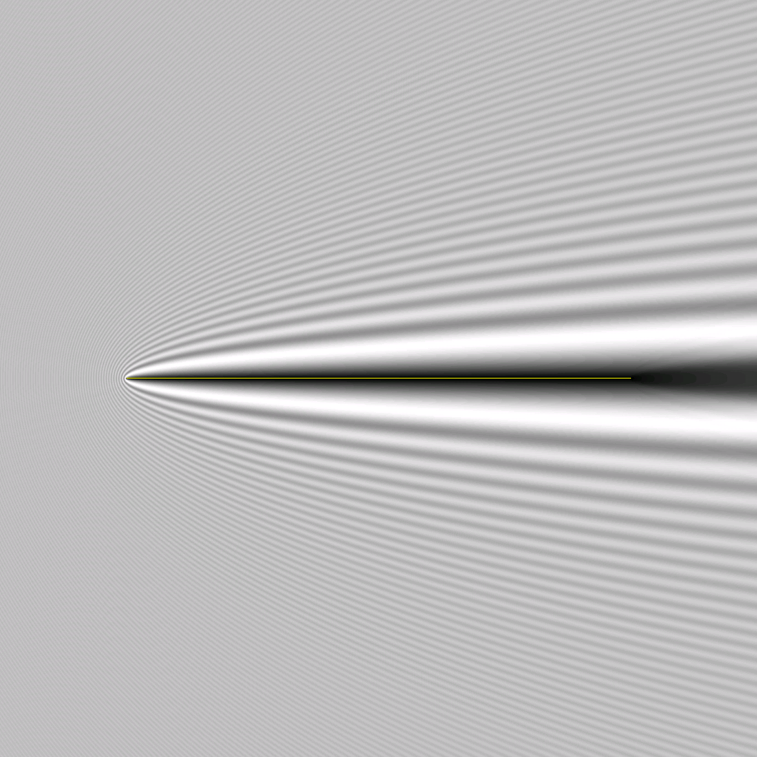
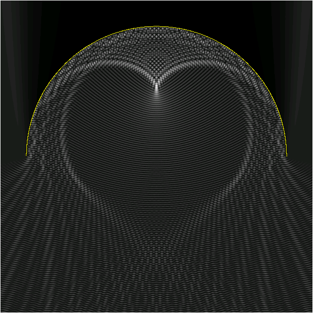
Figure 2: Sample diffraction patterns. Left: TE scattering (total field) by an infinitely thin strip of size $L=200\lambda$ for horizontal left-to-right incidence. (The TM total field at this incidence equals the incident field.) Right: TM solution for a half-circle of size $L=200\lambda$ under normal incidence from below. Note the trailing shadow in the wake of the strip, and the caustics inside the circular reflector.

4.6 Generalized Calderón formula

The generalized Calderón formula is obtained by expressing the combination $\tilde{N}\tilde{S}$ in the form

$$\tilde{N}\tilde{S}=\tilde{N}_{0}^{\tau}\tilde{S}_{0}^{\tau}+\tilde{K}=\tilde{J}_{0}^{\tau}+\tilde{K}$$ (46)

where the operator $\tilde{K}$, given by $\tilde{K}=\tilde{N}(\tilde{S}-\tilde{S}_{0}^{\tau})+(\tilde{N}-\tilde{N}_{0}^{\tau})\tilde{S}_{0}^{\tau},$ is compact in view of the classical Sobolev embedding theorems and the (increased) smoothness properties of the kernels of the operators $(\tilde{S}-\tilde{S}_{0}^{\tau})$ and $(\tilde{N}-\tilde{N}_{0}^{\tau})$ respectively. In view of the relation $\tilde{J}_{0}^{\tau}=\tilde{Z}_{0}^{-1}\tilde{J}_{0}\tilde{Z}_{0},$ $\tilde{J}_{0}$ and $\tilde{J}_{0}^{\tau}$ have the same spectrum: $(\lambda,v)$ is an eigenvalue-eigenvector pair for $\tilde{J}_{0}$ if and only if $(\lambda,\tilde{Z}_{0}^{-1}[v])$ is an eigenvalue-eigenvector pair for $\tilde{J}_{0}^{\tau}$. Clearly, $\tilde{J}_{0}^{\tau}$ has the same mapping properties and regularity as $\tilde{J}_{0}$ ($\tilde{J}_{0}^{\tau}$ is bicontinuous from $H^{s}_{e}(2\pi)$ into $H^{s}_{e}(2\pi)$), and therefore, the decomposition (46) shows that $\tilde{N}\tilde{S}$ equals the sum of an invertible bicontinuous operator and a compact operator; that is, $\tilde{N}\tilde{S}$ is a second-kind Fredholm operator.

5 High-Order Numerical Methods

In this section we present spectral quadrature rules for the operators $\tilde{S}$, $\tilde{N}$ and $\tilde{N}\tilde{S}$ which give rise to an efficient and accurate solver for the general open arc diffraction problem (1).

5.1 Spectral discretization for $\tilde{S}$

Use of the nodes $\left\{\theta_{n}=\frac{\pi(2n+1)}{2N}\right\}$, ${n=0,\cdots,N-1}$, gives rise [23, eq. (5.8.7),(5.8.8)] to a spectrally convergent cosine representation for smooth, $\pi$-periodic and even functions $\tilde{\varphi}$:

$$\begin{split}\tilde{\varphi}(\theta)=\sum_{n=0}^{N-1}a_{n}\cos(n\theta),\quad\mbox{where}\quad a_{n}=\frac{(2-\delta_{0n})}{N}\sum\limits_{j=0}^{N-1}\tilde{\varphi}(\theta_{j})\cos(n\theta_{j}).\end{split}$$ (47)

Thus, applying equation (21) to each term of expansion (47), we obtain the well-known spectral quadrature rule for the logarithmic kernel

$$\int_{0}^{\pi}\ln|\cos\theta-\cos\theta^{\prime}|\tilde{\varphi}(\theta^{\prime})d\theta^{\prime}\sim\frac{\pi}{N}\sum\limits_{j=0}^{N-1}\tilde{\varphi}(\theta_{j})R^{(N)}_{j}(\theta),$$ (48)

where

$$R^{(N)}_{j}(\theta)=-2\sum\limits_{m=0}^{N-1}(2-\delta_{m})\lambda_{m}\cos(m\theta_{j})\cos(m\theta).$$ (49)

Following [10, 18, 15] we then devise a high-order integration rule for the operator $\tilde{S}$, noting first from (2) and (36) that

$$\begin{split}G_{k}(\mathbf{r}(\theta),\mathbf{r}(\theta^{\prime}))=A_{1}(k,\cos\theta,\cos\theta^{\prime})\ln|\cos\theta-\cos\theta^{\prime}|+A_{2}(k,\cos\theta,\cos\theta^{\prime}),\end{split}$$ (50)

where, letting $R=|\mathbf{r}(\cos\theta)-\mathbf{r}(\cos\theta^{\prime})|$ we have

$$A_{1}(k,\cos\theta,\cos\theta^{\prime})=-\frac{1}{2\pi}J_{0}(kR),$$ (51)

and

$$A_{2}(k,\cos\theta,\cos\theta^{\prime})=\frac{i}{4}H^{1}_{0}(kR)+\frac{1}{2\pi}J_{0}(kR)\ln|\cos\theta-\cos\theta^{\prime}|.$$ (52)

In view of (37) and the smoothness of the ratio $\frac{R}{|\cos\theta-\cos\theta^{\prime}|}$, the functions $A_{1}$ and $A_{2}$ are even, smooth (analytic for analytic arcs) and $2\pi$-periodic functions of $\theta$ and $\theta^{\prime}$—and, thus, in view of (48), the expression

$$\begin{split}\int_{0}^{\pi}\tilde{\varphi}(\theta^{\prime})A_{1}(k,\cos\theta,\cos\theta^{\prime})\ln|\cos\theta-\cos\theta^{\prime}|\tau(\cos\theta^{\prime})d\theta^{\prime}\\ \sim\frac{\pi}{N}\sum_{j=0}^{N-1}\tilde{\varphi}(\theta_{j})\tau(\cos\theta_{j})A_{1}(k,\cos\theta,\cos\theta_{j})R^{(N)}_{j}(\theta)\end{split}$$ (53)

provides a spectrally accurate quadrature rule. By making use of trapezoidal integration for the second term in the right-hand side of (50) we therefore obtain the spectrally accurate quadrature approximation of the operator $\tilde{S}$ :

$$\begin{split}\tilde{S}[\varphi](\theta)\sim\frac{\pi}{N}\sum_{j=0}^{N-1}\tilde{\varphi}(\theta_{j})\tau(\cos\theta_{j})\big{(}A_{1}(k,\cos\theta,\cos\theta_{j})R^{(N)}_{j}(\theta)+A_{2}(k,\cos\theta,\cos\theta_{j})\big{)}.\end{split}$$ (54)

5.2 Efficient implementation

The right-hand side of (54) can be evaluated directly for all $\theta$ in the set of quadrature points $\left\{\theta_{n},n=0,\dots,N-1\right\}$ by means of a matrix-vector multiplication involving the matrix $S^{(N)}$ whose elements are defined by

$$\begin{split}S^{(N)}_{nj}=\frac{\pi}{N}\tau(\cos\theta_{j})\left(A_{1}(k,\cos\theta_{n},\cos\theta_{j})R^{(N)}_{j}(\theta_{n})+A_{2}(k,\cos\theta_{n},\cos\theta_{j})\right).\end{split}$$ (55)

A direct evaluation of the matrix $S^{(N)}$ on the basis of (49) requires $O(N^{3})$ operations; as shown in what follows, however, the matrix $S^{(N)}$ can be produced at significantly lower computational cost. Indeed, expressing the product of cosines in (49) as a sum of cosines of added and subtracted angles, the quantities

$$R^{(N)}_{j}(\theta_{n})=-\sum_{m=0}^{N-1}(2-\delta_{m})\lambda_{m}\big{(}\cos(\frac{m\pi}{N}|n-j|)+\cos(\frac{m\pi}{N}(n+j+1))\big{)}$$ (56)

can be expressed in the form

$$R^{N}_{j}(\theta_{n})=R^{(N)}(|n-j|)+R^{(N)}(n+j+1),$$ (57)

where the vector $R^{(N)}$ is given by

$$R^{(N)}(\ell)=-\sum_{m=0}^{N-1}(2-\delta_{m})\lambda_{m}\cos(\frac{m\pi}{N}\ell),\textbf{ }\ell\in[0,2N-1].$$ (58)

Our algorithm evaluates this vector efficiently by means of an FFT, and produces as a result the matrix $S^{(N)}$ at an overall computational cost of $O(N^{2}\ln N)$ operations. This fast spectrally-accurate algorithm could be further accelerated, if necessary, by means of techniques such as those presented in References [3, 6, 24].

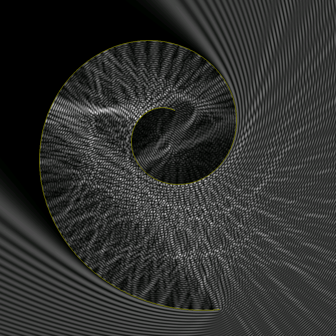
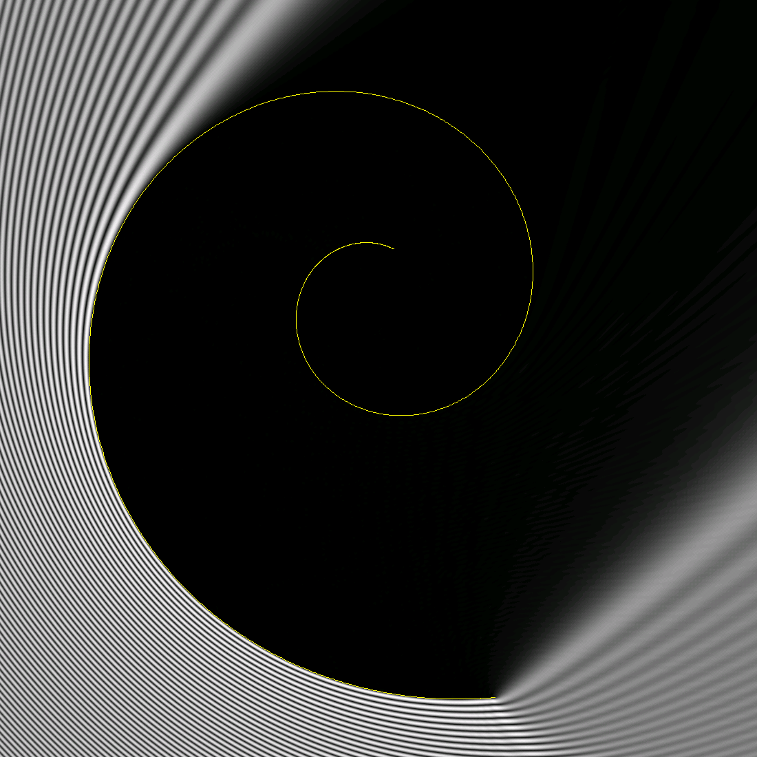
Figure 3: TE-diffraction by a spiral-shaped arc of size $L=200\lambda$, for incidence angles of 135^∘ (left) and 45^∘ (right) from the positive $x$-axis. The left figure shows internal reflections that enable the field to penetrate to the center of the spiral, giving rise to an interesting array of caustics. The relative error $\epsilon_{r}$ in both numerical solutions is no larger than $10^{-5}$.

5.3 Spectral Discretization for $\tilde{N}$

In order to evaluate $\tilde{N}$ we use (42), the first term of which is a single-layer operator which can be evaluated by means of a rule analogous to (54) and a rapidly computable matrix $N^{g,(N)}$ (similar to $S^{(N)}$) with elements

$$N^{g,(N)}_{nj}=\frac{k^{2}\pi}{N}\tau(\cos\theta_{j})\sin^{2}\theta_{j}(\mathbf{n}_{\theta_{j}}\cdot\mathbf{n}_{\theta_{n}})\left(A_{1}(k,\cos\theta_{n},\cos\theta_{j})R^{(N)}_{j}(\theta_{n})+A_{2}(k,\cos\theta_{n},\cos\theta_{j})\right).$$ (59)

To evaluate the second term in (42), in turn, we make use of the decomposition (44), and we approximate the quantity $\tilde{T}_{0}^{\tau}[\tilde{\varphi}]$ by means of term per term differentiation of the sine expansion of the function $\tilde{\varphi}(\theta)\sin(\theta)$ (which can itself be produced efficiently by means of an FFT). Since $\tilde{D}_{0}$ is essentially the differentiation operator in the $x$ variable,

$$\frac{1}{\sin\theta}\frac{d}{d\theta}\left(\varphi(\cos\theta)\right)=-\frac{d}{dx}\left(\varphi(x)\right),$$

our solver evaluates the quantity $\tilde{D}_{0}[\tilde{\varphi}]$ by invoking classical FFT-based Chebyshev differentiation rules [23, p. 195].

				TE($\tilde{S}$)		TE($\tilde{N}\tilde{S}$)
$\frac{L}{\lambda}$	N	$\epsilon_{r}$	Mat.	It.	Time	It.	Time
50	400	$<10^{-5}$	$<1s$	24	$<1s$	8	$<1s$
200	1600	$<10^{-5}$	$4s$	33	$1s$	8	$2s$
800	6400	$<10^{-5}$	$54s$	45	$18s$	8	$15s$

Table 2: Conditioning and computing times for the TE (Dirichlet) problem on the flat strip.

				TE($\tilde{S}$)		TE($\tilde{N}\tilde{S}$)
$\frac{L}{\lambda}$	N	$\epsilon_{r}$	Mat.	It.	Time	It.	Time
50	400	$<10^{-5}$	$<1s$	64	$<1s$	46	$<1s$
200	1600	$<10^{-5}$	$4s$	93	$3s$	62	$8s$
800	6400	$<10^{-5}$	$55s$	136	$58s$	79	$158s$

Table 3: Conditioning and computing times for the TE (Dirichlet) problem on the spiral-shaped arc.

				TM($\tilde{N})$		TM($\tilde{N}\tilde{S})$
$\frac{L}{\lambda}$	N	$\epsilon_{r}$	Mat.	It.	Time	It.	Time
50	400	$<10^{-5}$	$<1s$	67	$<1s$	9	$<1s$
200	1600	$<10^{-5}$	$4s$	160	$16s$	9	$1s$
800	6400	$<10^{-5}$	$55s$	298	$415s$	9	$17s$

Table 4: Conditioning and computing times for the TM (Neumann) problem on the strip.

				TM($\tilde{N})$		TM($\tilde{N}\tilde{S}$)
$\frac{L}{\lambda}$	N	$\epsilon_{r}$	Mat.	It.	Time	It.	Time
50	400	$<10^{-5}$	$<1s$	202	$<1s$	48	$<1s$
200	1600	$<10^{-5}$	$3s$	432	$65s$	63	$8s$
800	6400	$<10^{-5}$	$55s$	849	$1692s$	83	$160s$

Table 5: Conditioning and computing times for the TM (Neumann) problem on the spiral-shaped arc.

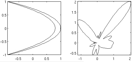
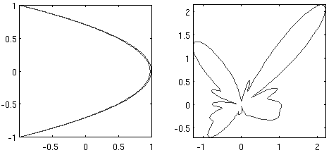
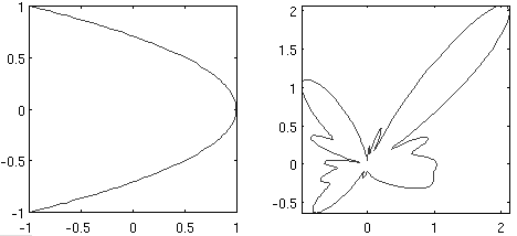
Figure 4: A sequence of increasingly thin closed curves converging to the open parabolic scatterer $x=1-2y^{2}$ and corresponding far-field patterns. From left to right: closed-curve with $a$=0.9, corresponding far field, closed-curve with $a$=0.99, corresponding far field, parabolic (open) arc and corresponding far field. Note the convergence of the far-field patterns as the closed scatterers approach the open parabolic scatterer.

6 Numerical Results

The numerical results presented in what follows were obtained by means of a C++ implementation of the quadrature rules introduced in Section 5 for numerical evaluation of the operators $\tilde{S}$ and $\tilde{N}$ (and thus, through composition, $\tilde{N}\tilde{S}$), in conjunction with the iterative linear algebra solver GMRES [25]. In all cases the errors reported were evaluated by comparisons with highly-resolved numerical solutions. All runs were performed in a single 2.2GHz Intel processor.

Spectral convergence. To demonstrate the high-order character of the algorithm described in previous sections we consider the problems of TE and TM scattering by the exponential spiral $x(s)=e^{s}\cos(5s)$, $y(s)=e^{s}\sin(5s)$ of size $\frac{L}{\lambda}=800$, where $L$ and $\lambda$ denote the perimeter of the curve and the electromagnetic wavelength, respectively. Table 1 demonstrates the spectral (exponentially-fast) convergence of the TE and TM numerical solutions produced by means of the operators $\tilde{S}$, $\tilde{N}$ and $\tilde{N}\tilde{S}$ for this problem (cf. equations (14) and (17) and (18)); note from Figure 3 the manifold caustics and multiple reflections associated with this solution.

Limit of Closed Curves. In order to obtain an indication of the manner in which an open arc problem can be viewed as a limit of closed-curve problems (and, in addition, to provide an independent verification of the validity of our solvers) we consider a test case in which the open-arc parabolic scatterer $x=1-2y^{2}$ is viewed as the limit as $a\rightarrow 1$ of the family of closed curves $x(s)=(1-a)\cos s+a\cos(2s)$, $y(s)=\sin(s).$ Using the closed-curve Nyström algorithms [10] we evaluate the TE fields scattered by these closed curves at $k=10$ for values of $a$ approaching $a=1$. Figure 4 displays the $k=10$ far fields corresponding to $a=0.9$ and $a=0.99$ side-by-side the corresponding far-field pattern for the limiting open parabolic arc as produced by the $\tilde{S}$-based open-arc solver. Clearly the closed-curve and open-arc solutions are quite close to each other. As might be expected, as $a$ approaches 1 an increasingly dense discretization is needed to maintain accuracy in the closed-curve solution: for $a=0.9$, 256 points where needed to reach a far field error of $10^{-4}$, while for $a=0.99$ as many 1024 points were needed to reach the same accuracy—even for the low frequency under consideration. The corresponding open-arc solution, in contrast, was produced with $10^{-4}$ accuracy by means of a much coarser, $64$ point discretization.

Solver performance. The TE (Dirichlet) problem can be solved by means of either the left-hand equation in (14) or equation (17), which in what follows are called equations TE$(\tilde{S})$ and TE$(\tilde{N}\tilde{S})$, respectively. The TM (Neumann) problem, similarly, can be tackled by means of either the right-hand equation in (14) or equation (18); we call these equations TM$(\tilde{N})$ and TM$(\tilde{N}\tilde{S})$, respectively. Results for TE and TM problems obtained by the various relevant equations for two representative geometries, a strip $[-1,1]$ and the exponential spiral mentioned above in this section, are presented in Figures 2 and 3 and Tables 2 through 5. In the tables the abbreviation “It.” denotes the number of iterations required to achieve an $\epsilon_{r}$ relative maximum error in the far field (calculated as the quotient of the maximum absolute error in the far field by the maximum absolute value of the far-field), “Mat.” is the time needed to build the $\tilde{S}$ matrix given by equation (55), as well as (when required) the corresponding matrix for $\tilde{N}^{g}$ which can be constructed in $O(N^{2})$ operations from the $\tilde{S}$ matrix (see Section 5), and “Time” is the total time required by the solver to find the solution once the matrix is stored.

As can be seen from these tables, the TM equation TM$(\tilde{N})$ requires very large number of iterations as the frequency grows and, thus, the computing times required by the low-iteration second-kind equation TM$(\tilde{N}\tilde{S})$ are significantly lower than those required by TM$(\tilde{N})$. The situation is reversed for the TE problem: although, the corresponding second-kind equation TE$(\tilde{N}\tilde{S})$ requires fewer iterations than TE$(\tilde{S})$, the total computational cost of the second-kind equation is generally higher in this case—since the application of the operator in TE$(\tilde{S})$ is significantly less expensive than the application of operator in TE$(\tilde{N}\tilde{S})$.

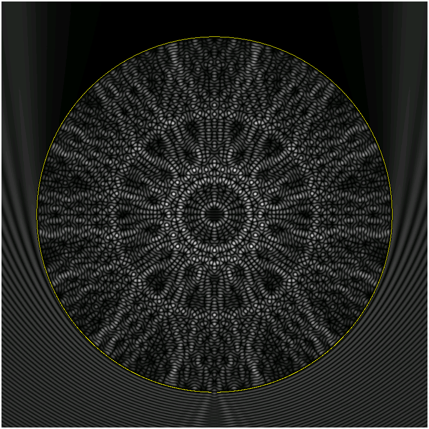
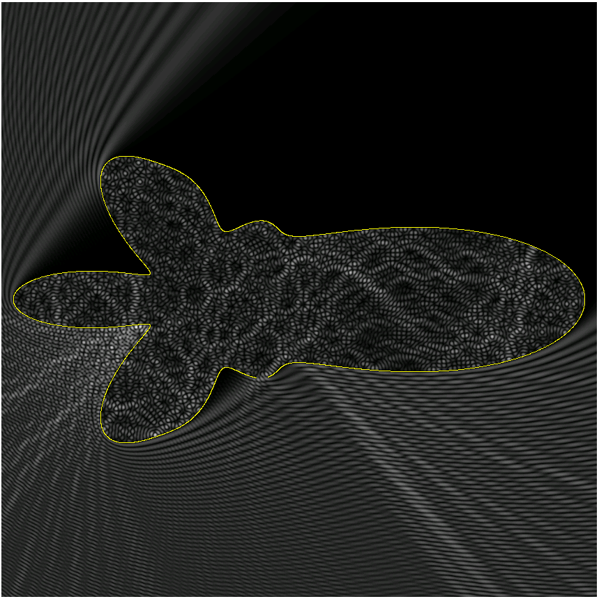
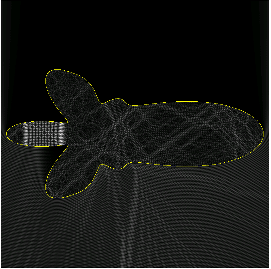
Figure 5: Left: TM polarization, for a circular cavity of size $\frac{L}{\lambda}=200$, with a bottom aperture of size equal to the wavelength $\lambda$. Center: TE problem for a rocket-shaped cavity with perimeter $L=200\lambda$, and a bottom aperture equal to $6\lambda$. Right: same as in the center figure, but in the case of normal incidence—for which a strong resonance develops in the tail of the rocket.

Resonant Cavities. We have found that interesting resonant electromagnetic behavior arises from diffractive elements constructed as almost-closed open-arcs. As can be seen in Figure 5, for example, circular and rocket-shaped cavities with small openings (a few wavelengths in size), can give rise to interesting and highly energetic field patterns within the open cavity. The number of iterations required for each of these configurations is of course much larger than for simpler geometries, such as the strip. Yet, overall reduction in number of iterations and computing times is observed when the equation TM$(\tilde{N}\tilde{S})$ is used in lieu of TM$(\tilde{N})$. For the TE problem, once again TE$(\tilde{S})$ gives rise to faster overall numerics than TE$(\tilde{N}\tilde{S})$, although the latter equation still requires fewer GMRES iterations.

$\frac{L}{\lambda}$	N	$\epsilon_{r}$	It.	Mat. Time	Sol. Time
50	400	$1.2\times 10^{-5}$	124	$<1s$	$1s$
200	1600	$6.3\times 10^{-6}$	293	$3s$	$15s$
800	6400	$2.2\times 10^{-5}$	672	$56s$	$411s$

Table 6: Conditioning and times for the solution of the Dirichlet problem using the generalization of the method [2, 13]: $(\tilde{S}_{0}^{\tau})^{-1}$ as a preconditioner for the spiral-shaped arc.

Conclusions. We have introduced new second kind equations and associated numerical algorithms for solution of TE and TM scattering problems by open arcs. The new open-arc second-kind formulations are the first ones in the literature that lead to reduced number of GMRES iterations consistently across various geometries and frequency regimes. The new second-kind formulation TM$(\tilde{N}\tilde{S})$ is highly beneficial for the TM problem, giving rise to order-of-magnitude improvements in computing times over the hypersingular formulation TM$(\tilde{N})$. Such gains do not occur in the TE case: although, the second-kind equation TE$(\tilde{N}\tilde{S})$ requires fewer iterations than TE$(\tilde{S})$, the total computational cost of the second-kind equation is generally higher in this case—since the application of the operator in TE$(\tilde{S})$ is significantly less expensive than the application of operator in TE$(\tilde{N}\tilde{S})$. Generalization of these methods enabling efficient second-kind solution of problems of scattering by open-surfaces in three dimensions will be presented elsewhere [7].

Acknowledgments. The authors gratefully acknowledge support from AFOSR, NSF, JPL and the Betty and Gordon Moore Foundation.

References

- [1] Xavier Antoine, Abderrahmane Bendali, and Marion Darbas. Analytic preconditioners for the boundary integral solution of the scattering of acoustic waves by open surfaces. J. Comput. Acoust., 13(3):477–498, 2005.
- [2] K. Atkinson and I. Sloan. The numerical solution of first-kind logarithmic-kernel integral equations on smooth open arcs. Math. Comp., 56(193):119–139, 1991.
- [3] E Bleszynski, M Bleszynski, and T Jaroszewicz. AIM: Adaptive integral method for solving large-scale electromagnetic scattering and radiation problems. Radio Sci., 31(5):1225–1251, 1996.
- [4] A. Brown, P. R. Halmos, and A. L. Shields. Cesàro operators. Acta Sci. Math. (Szeged), 26:125–137, 1965.
- [5] O. Bruno and M. Haslam. Regularity theory and superalgebraic solvers for wire antenna problems. SIAM J. Sci. Comput., 29(4):1375–1402, 2007.
- [6] O. Bruno and L. Kunyansky. A fast, high-order algorithm for the solution of surface scattering problems: basic implementation, tests, and applications. J. Comput. Phys., 169(1):80–110, 2001.
- [7] O. Bruno and S. Lintner. A high-order integral solver for scalar problems of diffraction by screens and apertures in three dimensional space. In preparation.
- [8] S. H. Christiansen and J.-C. Nédélec. Preconditioners for the boundary element method in acoustics. In Mathematical and numerical aspects of wave propagation (Santiago de Compostela, 2000), pages 776–781. SIAM, Philadelphia, PA, 2000.
- [9] D. Colton and R. Kress. Integral Equation Methods in Scattering Theory. John Wiley & Sons, 1983.
- [10] D. Colton and R. Kress. Inverse Acoustic and Electromagnetic Scattering Theory. Springer, 1997.
- [11] A. Erdélyi, W. Magnus, F. Oberhettinger, and F. Tricomi. Higher transcendental functions. Vol. II. Robert E. Krieger Publishing Co. Inc., Melbourne, Fla., 1981. Based on notes left by Harry Bateman, Reprint of the 1953 original.
- [12] George C. Hsiao, Ernst P. Stephan, and Wolfgang L. Wendland. On the Dirichlet problem in elasticity for a domain exterior to an arc. J. Comput. Appl. Math., 34(1):1–19, 1991.
- [13] S. Jiang and V. Rokhlin. Second kind integral equations for the classical potential theory on open surfaces. II. J. Comput. Phys., 195(1):1–16, 2004.
- [14] R. Kress. Linear integral equations, volume 82 of Applied Mathematical Sciences. Springer-Verlag, New York, second edition, 1999.
- [15] R. Kussmaul. Ein numerisches Verfahren zur Lösung des Neumannschen Neumannschen Aussenraumproblems für die Helmholtzsche Schwingungsgleichung. Computing (Arch. Elektron. Rechnen), 4:246–273, 1969.
- [16] S. Lintner and O. Bruno. A generalized Calderón formula for open-arc diffraction problems: theoretical considerations. Submitted.
- [17] R. Duduchava M. Costabel, M. Dauge. Asymptotics without logarithmic terms for crack problems. Communications in PDE, pages 869–926, 2003.
- [18] Erich Martensen. Über eine Methode zum räumlichen Neumannschen Problem mit einer Anwendung für torusartige Berandungen. Acta Math., 109:75–135, 1963.
- [19] J. C. Mason and D. C. Handscomb. Chebyshev polynomials. Chapman & Hall/CRC, Boca Raton, FL, 2003.
- [20] L. Mönch. On the numerical solution of the direct scattering problem for an open sound-hard arc. J. Comput. Appl. Math., 71(2):343–356, 1996.
- [21] JC. Nédélec. Acoustic and electromagnetic equations, volume 144 of Applied Mathematical Sciences. Springer-Verlag, New York, 2001.
- [22] A. Ya. Povzner and I. V. Suharevskiĭ. Integral equations of the second kind in problems of diffraction by an infinitely thin screen. Soviet Physics. Dokl., 4:798–801, 1960.
- [23] W. H. Press, Teukolsky S., W. Vetterling, and B. Flannery. Numerical Recipes in C. Cambridge University Press, 1992. Second Edition.
- [24] V. Rokhlin. Diagonal forms of translation operators for the Helmholtz equation in three dimensions. Appl. Comput. Harmon. Anal., 1(1):82–93, 1993.
- [25] Youcef Saad and Martin H. Schultz. GMRES: a generalized minimal residual algorithm for solving nonsymmetric linear systems. SIAM J. Sci. Statist. Comput., 7(3):856–869, 1986.
- [26] J. Saranen and G. Vainikko. Periodic integral and pseudodifferential equations with numerical approximation. Springer Monographs in Mathematics. Springer-Verlag, Berlin, 2002.
- [27] E. Stephan. Boundary integral equations for screen problems in . Integral Equations Operator Theory, 10(2):236–257, 1987.
- [28] E. Stephan and T. Tran. Domain decomposition algorithms for indefininte hypersingular integral equations: the h and p versions. SIAM J. Sci. Comp., 19(4):1139–1153, 1998.
- [29] E. Stephan and W. Wendland. An augmented Galerkin procedure for the boundary integral method applied to two-dimensional screen and crack problems. Applicable Anal., 18(3):183–219, 1984.
- [30] W. L. Wendland and E. P. Stephan. A hypersingular boundary integral method for two-dimensional screen and crack problems. Arch. Rational Mech. Anal., 112(4):363–390, 1990.
- [31] Y. Yan and I. H. Sloan. On integral equations of the first kind with logarithmic kernels. J. Integral Equations Appl., 1(4):549–579, 1988.