The open-faced sandwich adjustment for MCMC using estimating functions

Abstract

The situation frequently arises where working with the likelihood function is problematic. This can happen for several reasons—perhaps the likelihood is prohibitively computationally expensive, perhaps it lacks some robustness property, or perhaps it is simply not known for the model under consideration. In these cases, it is often possible to specify alternative functions of the parameters and the data that can be maximized to obtain asymptotically normal estimates. However, these scenarios present obvious problems if one is interested in applying Bayesian techniques. Here we describe open-faced sandwich adjustment, a way to incorporate a wide class of non-likelihood objective functions within Bayesian-like models to obtain asymptotically valid parameter estimates and inference via MCMC. Two simulation examples show that the method provides accurate frequentist uncertainty estimates. The open-faced sandwich adjustment is applied to a Poisson spatio-temporal model to analyze an ornithology dataset from the citizen science initiative eBird.

1 Introduction

For many models arising in various fields of statistical analysis, working with the likelihood function can be undesirable. This may be the case for several reasons—perhaps the likelihood is prohibitively expensive to compute, perhaps it presumes knowledge of a component of the model that one is unwilling to specify, or perhaps its form is not even known for a chosen probability model. Such scenarios present problems if one wishes to perform Bayesian analysis. Applying the Bayesian computational and inferential machinery, thereby enjoying benefits such as natural shrinkage, variance propagation, and the ability to incorporate complex hierarchical dependences, usually requires working directly with the likelihood function.

To motivate the development, we briefly describe the analysis of bird sightings contained in Section 5.1. The data consist of several thousand counts occurring irregularly in space and time (see Figure 1), along with several spatially-varying covariates carefully chosen by a group of ornithologists. A natural model for such data is a hierarchical Poisson regression with a random effect specified as a spatio-temporal Gaussian process with unknown covariance parameters. Here, whetever one’s philosophical orientation, Bayesian methods are most practical to implement, and in addition provide sharing of information across space and time, as well as automatic uncertainty estimation of predictive abundance maps. Furthermore, obtaining an MCMC sample of the posterior distribution is desirable because inferences on the posterior correlation surface of the random effect, a nonlinear functional of random covariance parameters, is of independent interest to the ornithologists. However, the sheer size of the dataset makes MCMC under this model intractable, so a faster objective function is used in place of the high-dimensional Gaussian likelihood. The goal of the method presented here is to enable such a substitution while retaining a valid interpretation of the resultant MCMC sample.

Figure 1: Spatial locations of Northern Cardinal observations.

More generally, suppose that one specifies a model, either one-stage or hierarchical, and wants the advantages of being Bayesian, but the likelihood in some level of the hierarchy is problematic. Suppose, however, that one can write down some objective function $\ell_{M}(\boldsymbol{\theta};\mathbf{y})$ of the parameters and the data (possibly conditional on other parameters) that behaves similarly to the log likelihood. We will define what we mean by “similarly” in Section 2. Important examples of methods that employ such objective functions include generalized estimating equations (Hardin and Hilbe, 2003), generalized method of moments (Hall, 2005), and robust M-estimation (Huber and Ronchetti, 2009), as well as the two examples we will consider here, covariance tapering (Kaufman et al., 2008) and composite likelihoods (Lindsay, 1988).

The question we attempt to answer here is this: Can we insert $\ell_{M}(\boldsymbol{\theta};\mathbf{y})$, in place of the likelihood, into an MCMC algorithm like Metropolis-Hastings and “trick” it into doing something useful? We claim that we can—that for many useful examples, simply swapping $\ell_{M}(\boldsymbol{\theta};\mathbf{y})$ into a sampler results in a quasi-posterior sample that can be rotated and scaled to yield desirable properties.

The OFS adjustment relies on asymptotic theory that was formally developed in Chernozhukov and Hong (2003), but which is quite intuitive. These authors were interested in using Metropolis-Hastings as an optimization algorithm for badly-behaved objective functions, not in using non-likelihood objective functions for performing Bayesian-like analysis, as we are here. Although their goals were entirely different, the theory contained therein is extremely useful for our purposes.

Previous attempts to incorporate non-likelihood objective functions into the Bayesian setting, to our knowledge, have been few. McVean et al. (2004) use composite likelihoods within reversible jump MCMC, without any adjustment, to estimate population genetic parameters. Realizing that their sampler would result in invalid inferences, McVean et al. (2004) turn to a parametric bootstrap to estimate sampling variability. Smith and Stephenson (2009) were interested in max-stable processes for spatial extreme value analysis. They also use composite likelihoods within MCMC without adjustment. The special case of using the generalized method of moments objective function (Hansen, 1982; Hall, 2005) for generalized linear models within an MCMC sampler was explored by Yin (2009). Tangentially related is Tian et al. (2007), who use MCMC to estimate the sampling distribution of $\hat{\boldsymbol{\theta}}=\operatornamewithlimits{argmax}{\ell_{M}(\boldsymbol{\theta};\mathbf{y})}$.

Cooley et al. (2012) attempt to solve the same problem that we address here. Whereas we adjust quasi-posterior samples generated from MCMC post hoc, these authors propose an adjustment to the Metropolis likelihood ratio within the sampler itself. Their goal, like ours, is to achieve desirable frequentist coverage properties of credible intervals computed based on MCMC. Although their approach is quite general, Cooley et al. (2012) restrict their attention to using composite likelihoods for max-stable processes. The approach taken in the present article is closely related to that of Cooley et al. (2012), but the OFS adjustment differs from their adjustment in its structure as well as its motivating asymptotic arguments.

Both the motivating insights for the OFS adjustment and the criterion by which we evaluate it is essentially the idea of calibration (Draper, 2006). In our interpretation, a well-calibrated method has the property that when used to construct credible intervals from many different datasets, those intervals ought to cover the true parameter at close to their nominal rates. Essentially, this says that well-calibrated credible intervals behave like confidence intervals. If we construct intervals with accurate coverage directly as the $\alpha/2$ and $(1-\alpha/2)$ empirical quantiles of an MCMC sample for different values of $\alpha$, we claim that in some way our uncertainty about a parameter is well-described by the sample. Evaluating an approximate Bayesian method by this criterion has intuitive practical appeal, and it has been endorsed in particular by objective Bayesians (Bayarri and Berger, 2004; Berger et al., 2001, e.g.).

This principle, along with some basic asymptotic observations, leads to the OFS adjustment. The asymptotic theory gives us the limiting normal distribution of quasi-Bayes point estimators. We take this distribution, in an informal sense, to be a summary of our uncertainty about $\boldsymbol{\theta}$, up to an asymptotic approximation. The asymptotic theory also gives us the limiting normal distribution of the quasi-posterior. Since these two limiting distributions are not, in general, the same, and since we would like the quasi-posterior to summarize our uncertainty about $\boldsymbol{\theta}$ in the sense of being well-calibrated, our strategy is to adjust samples from the quasi-posterior so that their limiting distribution matches that of the quasi-Bayesian point estimator.

We note the temptation to ask how well the adjusted quasi-posterior distribution approximates the true posterior distribution, in cases when the true likelihood is available. However, this is the incorrect comparison to make. The true posterior distribution contains the information about $\boldsymbol{\theta}$ obtained through the likelihood. When some other function $\ell_{M}$ is used in place of the likelihood, there is no reason to expect the information content to remain the same. We would like the adjusted quasi-posterior distribution to represent this loss of information, not hide it. In our simulation examples in Section 4, the frequentist accuracy of credible intervals based on adjusted quasi-posterior samples shows that the OFS adjustment accomplishes this task.

Throughout, it will be assumed that expectations will be computed with respect to the true parameter $\boldsymbol{\theta}_{0}$. We define the square root of a symmetric positive definite matrix $\mathbf{A}$ to be $\mathbf{A}^{1/2}$ = $\mathbf{OD}^{1/2}\mathbf{O}^{\prime}$, where $\mathbf{A=ODO^{\prime}}$ with $\mathbf{O}$ orthogonal and $\mathbf{D}$ diagonal. The square root of a matrix is not unique; here we compute $\mathbf{A}^{1/2}$ using the singular value decomposition, which is numerically stable and preserves key geometric attributes.

We begin in Section 2 by defining the quasi-Bayesian framework and reviewing the relevant asymptotic theory. In Section 3 we develop the OFS adjustment method, and we demonstrate how to apply it in two different statistical contexts in Section 4. In Section 5 we apply the OFS adjustment to analyze a dataset of Northern Cardinal sightings taken from the citizen science project eBird. Section 6 concludes.

2 The quasi-Bayesian framework

We begin by assuming that the parameter of interest $\boldsymbol{\theta}$ lies in the interior of a compact convex space $\boldsymbol{\Theta}$. Suppose we are given $\mathbf{y}$, which consists of $n$ observations, from which we wish to estimate $\boldsymbol{\theta}$. Suppose further that we have at our disposal some objective function $\ell_{M}(\boldsymbol{\theta};\mathbf{y})$ from which it is possible to compute $\hat{\boldsymbol{\theta}}_{M}=\operatornamewithlimits{argmax}_{\boldsymbol{\Theta}}{\ell_{M}(\boldsymbol{\theta};\mathbf{y})}$.

Following Chernozhukov and Hong (2003), we define the quasi-posterior distribution based on $n$ observations as

$$\pi_{M,n}(\boldsymbol{\theta}|\mathbf{y}_{n})=\frac{L_{M,n}(\boldsymbol{\theta};\mathbf{y}_{n})\pi(\boldsymbol{\theta})}{\int_{\Theta}L_{M,n}(\boldsymbol{\theta};\mathbf{y}_{n})\pi(\boldsymbol{\theta})\,\mathrm{d}\boldsymbol{\theta}},$$ (1)

where $L_{M,n}(\boldsymbol{\theta};\mathbf{y}_{n})=\exp{\{\ell_{M,n}(\boldsymbol{\theta};\mathbf{y}_{n})\}}$, and $\pi(\boldsymbol{\theta})$ is a prior density on $\boldsymbol{\theta}$. We will assume, for convenience, that $\pi(\boldsymbol{\theta})$ is proper with support on $\boldsymbol{\Theta}$. The function $L_{M,n}$ is not necessarily a density, and thus $\pi_{M,n}(\boldsymbol{\theta}|\mathbf{y}_{n})$ is not a true posterior density in any probabilistic sense. We will assume, however, that $L_{M,n}$ is integrable, so as long as the prior $\pi(\boldsymbol{\theta})$ is proper, it easily follows that $\pi_{M,n}(\boldsymbol{\theta}|\mathbf{y}_{n})$ will be a proper density.

Equipped with notion of a quasi-posterior density, we can define quasi-posterior risk as $R_{n}(\boldsymbol{\theta})=\int_{\boldsymbol{\Theta}}\!\rho_{n}(\boldsymbol{\theta}-\boldsymbol{\theta}^{*})\pi_{M,n}(\boldsymbol{\theta}^{*}|\mathbf{y}_{n})\,\mbox{d}\boldsymbol{\theta}^{*}$, where $\rho_{n}(\mathbf{u})$ is some convex scalar loss function. For simplicity, we assume that $\rho_{n}(\mathbf{u})$ is symmetric, although this assumption may be dropped. Then for a given loss function, the quasi-Bayes estimator is naturally defined as $\hat{\boldsymbol{\theta}}_{\text{QB}}$ $\,=\operatornamewithlimits{argmin}_{\boldsymbol{\theta}\in\boldsymbol{\Theta}}R_{n}(\boldsymbol{\theta})$, the value of $\boldsymbol{\theta}$ that minimizes quasi-posterior risk.

Our requirements on $\ell_{M,n}(\boldsymbol{\theta};\mathbf{y}_{n})$ are fairly minimal and are met by most objective functions in wide use in statistics. Technical assumptions are contained in Chernozhukov and Hong (2003), but they are in general satisfied when $\hat{\boldsymbol{\theta}}_{M}$ is weakly consistent for $\boldsymbol{\theta}_{0}$ and asymptotically normal.

Asymptotic normality of $\hat{\boldsymbol{\theta}}_{M}$ is of the form

$$\mathbf{J}_{n}^{1/2}(\hat{\boldsymbol{\theta}}_{M,n}-\boldsymbol{\theta}_{0})\xrightarrow{\mathscr{D}}N(\mathbf{0,I}),$$ (2)

where

$$\mathbf{J}_{n} =\mathbf{Q}_{n}\mathbf{P}^{-1}_{n}\mathbf{Q}_{n}$$

$$\mathbf{P}_{n} =\mbox{E}_{0}[\nabla_{0}\ell_{M,n}\nabla_{0}\ell_{M,n}^{\prime}]$$

$$\mathbf{Q}_{n} =-\text{E}_{0}[\mathcal{H}_{0}\ell_{M,n}].$$ (3)

The notation $\nabla_{0}f$ refers to the gradient of the function $f$ evaluated at the true parameter $\boldsymbol{\theta}_{0}$, and $\mathcal{H}_{0}f$ refers to the Hessian of $f$ evaluated at $\boldsymbol{\theta}_{0}$. These matrices have been defined in terms of partial derivatives, but in general, $\ell_{M,n}$ does not have to be differentiable or even continuous for the theory to apply. In this case, small adjustments of the definitions of $\mathbf{P}_{n}$ and $\mathbf{Q}_{n}$ are necessary.

The sandwich matrix $\mathbf{J}^{-1}_{n}$ is familiar from generalized estimating equations, quasi-likelihood, and other areas, and is referred to by various names, including the Godambe information criterion and the robust information criterion (e.g. Durbin, 1960; Bhapkar, 1972; Morton, 1981; Ferreira, 1982; Godambe and Heyde, 1987; Heyde, 1997). We note that in the special case when $\ell_{M,n}(\boldsymbol{\theta};\mathbf{y})$ is the true likelihood, $\mathbf{Q}_{n}\equiv\mathbf{J}_{n}$, the Fisher information. We will hereafter assume that this is not the case.

2.1 Review of relevant asymptotic theory

Chernozhukov and Hong (2003) elucidates the asymptotic behavior of $\pi_{M,n}(\boldsymbol{\theta}|\mathbf{y}_{n})$, which motivates the open-face sandwich adjustment. These results are direct analogues of well-known asymptotic properties of true posterior distributions. Their Theorem 2, which we re-state below, states that the asymptotic distribution of the quasi-Bayes estimator $\hat{\boldsymbol{\theta}}_{\text{QB},n}$ is the same as that of the extremum estimator $\hat{\boldsymbol{\theta}}_{M,n}$.

Theorem 1

Assuming sufficient regularity of $\ell_{M,n}(\boldsymbol{\theta};\mathbf{y}_{n})$,

$$\mathbf{J}_{n}^{1/2}(\hat{\boldsymbol{\theta}}_{\text{QB}}-\boldsymbol{\theta}_{0})\xrightarrow{\mathscr{D}}N(\mathbf{0,I}).$$

Theorem 1 above is the quasi-posterior extension of the well-known result that, under fairly general conditions, Bayesian point estimates have the same asymptotic distribution as maximum likelihood estimates.

Theorem 1 of Chernozhukov and Hong (2003), which we re-state here in a slightly different form, is a kind of quasi-Bayesian consistency result, showing that quasi-posterior mass accumulates at the true parameter $\boldsymbol{\theta}_{0}$.

Theorem 2

Under the same conditions as Theorem 1

$$\|\pi_{M,n}(\boldsymbol{\theta}|\mathbf{y}_{n})-\pi_{M,\infty}(\boldsymbol{\theta}|\mathbf{y}_{n})\|_{\text{TV}}\xrightarrow{\mathscr{P}}0,$$

where $\|\cdot\|_{\text{TV}}$ indicates the total variation norm, and $\pi_{M,\infty}(\boldsymbol{\theta}|\mathbf{y}_{n})$ is a normal density with random mean $\boldsymbol{\theta}_{0}+\mathbf{Q}_{n}^{-1}\nabla\boldsymbol{\ell}_{M,n}(\boldsymbol{\theta}_{0})$ and covariance matrix $\mathbf{Q}_{n}^{-1}$.

Theorem 2 may be arrived at informally via a simple Taylor series argument. It is therefore intuitive that the quasi-posterior converges to limiting normal distribution whose covariance matrix is defined by the second derivatives of $\ell_{\text{M}}$.

The key observation is that the limiting quasi-posterior distribution has a different covariance matrix than the asymptotic sampling distribution of the quasi-Bayes point estimate. The consequence is that the usual Bayesian method of constructing credible intervals based on quantiles of the quasi-posterior sample will, viewed as confidence intervals, not have their nominal frequentist coverage probabilities. Fortunately, thanks to Chernozhukov and Hong (2003), we know what those two asymptotic covariance matrices look like, which suggests a way to “fix” $\pi_{M,n}(\boldsymbol{\theta}|\mathbf{y}_{n})$.

3 The open-faced sandwich adjustment

Let us assume that we have a sample of draws from $\pi_{M,n}(\boldsymbol{\theta}|\mathbf{y}_{n})$, generated by replacing the likelihood with $\ell_{M}(\boldsymbol{\theta};\mathbf{y})$ in some MCMC sampler such as Metropolis-Hastings. Our aim here is to adjust the quasi-posterior draws such that the adjusted sample realistically reflects how the data informs our uncertainty about the parameter of interest $\boldsymbol{\theta}$ through the function $\ell_{M}(\boldsymbol{\theta};\mathbf{y})$. Were that the case, the usual credible intervals constructed from empirical quantiles of the adjusted sample would have close to nominal coverage. We will accomplish this by constructing a matrix $\boldsymbol{\Omega}_{n}$ that, when applied to the (centered) quasi-posterior sample, will rotate and scale the points in an appropriate way.

We have observed that whereas the asymptotic covariance matrix of $\hat{\boldsymbol{\theta}}_{M,n}$ is the sandwich matrix $\mathbf{J}_{n}^{-1}$, the asymptotic covariance matrix of the quasi-posterior distribution is a single “slice of bread” $\mathbf{Q}_{n}^{-1}$. What we want to do then is complete the sandwich by joining the slice of bread $\mathbf{Q}_{n}^{-1}$ to the open-faced sandwich $\mathbf{P}_{n}\mathbf{Q}_{n}^{-1}$ to get $\mathbf{J}_{n}^{-1}$.

We define $\boldsymbol{\Omega}_{n}=\mathbf{Q}_{n}^{-1}\mathbf{P}_{n}^{1/2}\mathbf{Q}_{n}^{1/2}$, the open-faced sandwich adjustment matrix. One can easily check that if $\mathbf{Z}_{n}\sim N(\mathbf{0},\mathbf{Q}_{n}^{-1})$, then $\boldsymbol{\Omega}_{n}\mathbf{Z}_{n}\sim N(\mathbf{0},\mathbf{J}_{n}^{-1})$. The idea then is to take samples from $\pi_{M}(\boldsymbol{\theta}|\mathbf{y})$ obtained via MCMC and pre-multiply them (after centering) by an estimator $\hat{\boldsymbol{\Omega}}$ of $\boldsymbol{\Omega}$ to “correct” the quasi-posterior sample. That is, if $\boldsymbol{\theta}^{(1)},\ldots,\boldsymbol{\theta}^{(J)}$ is a sample from $\pi_{M}(\boldsymbol{\theta}|\mathbf{y})$, then for each $j=1,\ldots,J$,

$$\boldsymbol{\theta}_{\text{OFS}}^{(j)}=\hat{\boldsymbol{\theta}}_{\text{QB}}+\hat{\boldsymbol{\Omega}}(\boldsymbol{\theta}^{(j)}-\hat{\boldsymbol{\theta}}_{\text{QB}})$$ (4)

is the open-face sandwich adjusted sample. It is clear that a consistent estimator of $\boldsymbol{\Omega}$ will generate credible intervals that are consistent $(1-\alpha)$ confidence intervals.

3.1 Estimating $\boldsymbol{\Omega}$

The OFS adjustment (4) requires an estimate of the matrix $\boldsymbol{\Omega}$, which in turn requires estimates of $\mathbf{P}$ and $\mathbf{Q}$. Because the OFS adjustment occurs post-hoc, it is possible to leverage the existing MCMC sample to compute $\hat{\boldsymbol{\Omega}}$. There are many possible approaches to this task, and here we offer some suggestions, which we summarize in Table 1.

While is $\mathbf{P}$ is notoriously difficult to estimate well (see Kauermann and Carroll, 2001, for some examples), Theorem 1 immediately suggests a way to estimate $\mathbf{Q}$ directly from the MCMC sample with almost no additional computational cost. Specifically, noting that the quasi-posterior density converges to a normal with covariance matrix $\mathbf{Q}^{-1}$, a natural estimate $\hat{\mathbf{Q}}^{-1}_{\text{I}}$ is just the sample covariance matrix of the MCMC sample. Another possibility that requires almost no additional computation is to retain the results of the evaluations of $\ell_{M}$ at each iteration of the sampler and use them to numerically estimate the Hessian matrix at $\hat{\boldsymbol{\theta}}_{\text{QB}}$. This Hessian approximation will generally be a good estimator $\hat{\mathbf{Q}}_{\text{II}}$ of $\mathbf{Q}$.

These estimators of $\mathbf{Q}$ are not only simple to compute, but they arise as direct results of MCMC output, requiring no additional analytical derivations based on $\ell_{M}$. They are, in this sense, “model-blind.” Unfortunately, we are unaware of any such “model-blind” estimators of $\mathbf{P}$. The simplest solution, in the case where we can write an expression for $\nabla\ell_{M}(\boldsymbol{\theta};\mathbf{y})$ and the data $\mathbf{y}$ consists of $n$ independent replicates, is to compute a basic moment estimator

$$\hat{\mathbf{P}}_{\text{I}}=\frac{1}{n}\sum_{i=1}^{n}\nabla\ell_{M}(\hat{\boldsymbol{\theta}}_{\text{QB}};\mathbf{y}_{i})\nabla\ell_{M}(\hat{\boldsymbol{\theta}}_{\text{QB}};\mathbf{y}_{i})^{\prime},$$ (5)

which is consistent as $n\rightarrow\infty$ under standard regularity conditions. We use equation (5) in Section and 4.2, where we have replication. However, because $\nabla\ell_{M}(\hat{\boldsymbol{\theta}}_{\text{QB}};\mathbf{y})$ converges to zero, when we only observe a single realization of a stochastic process, as in Section 4.1, equation (5) fails to provide a viable estimator. In this latter example, analytical expressions for $\mathbf{P}(\boldsymbol{\theta})$ are available. Plugging $\hat{\boldsymbol{\theta}}_{\text{QB}}$ into the analytical asymptotic expression gives an estimator $\hat{\mathbf{P}}_{\text{II}}$. If a corresponding analytical expression exists for $\mathbf{Q}$, we call the corresponding plug-in estimator $\hat{\mathbf{Q}}_{\text{III}}$

When an expression for $\mathbf{P}(\boldsymbol{\theta})$ is unavailable, but when it is possible to simulate the process that generated $\mathbf{y}$, the parametric bootstrap is an attractive option. Let $\mathbf{y}_{1},\ldots,\mathbf{y}_{K}$ be $K$ independent realizations of the stochastic process generated under $\hat{\boldsymbol{\theta}}_{\text{QB}}$. Then

$$\hat{\mathbf{P}}_{\text{boot}}=\frac{1}{K}\sum_{k=1}^{K}\nabla\ell_{M}(\hat{\boldsymbol{\theta}}_{\text{QB}};\mathbf{y}_{k})\nabla\ell_{M}(\hat{\boldsymbol{\theta}}_{\text{QB}};\mathbf{y}_{k})^{\prime}$$ (6)

is the parametric bootstrap estimator of $\mathbf{P}$ (an analogous estimator could, of course, be used for $\mathbf{Q}$). A nice feature of (5) and (6) is that, at the expense of (perhaps considerable) computational effort, one could substitute finite-difference approximations to the required gradients to obtain reasonable estimators, even in the absence of available closed-form expressions for $\nabla\ell_{M}(\boldsymbol{\theta};\mathbf{y})$.

Estimator	Description
$\hat{\mathbf{Q}}_{\text{I}}^{-1}$	sample covariance of MCMC sample
$\hat{\mathbf{Q}}_{\text{II}}$	Hessian of $\ell_{M}(\hat{\boldsymbol{\theta}}_{\text{QB}})$
$\hat{\mathbf{Q}}_{\text{III}}$	plug $\hat{\boldsymbol{\theta}}_{\text{QB}}$ into asymptotic formula
$\hat{\mathbf{P}}_{\text{I}}$	moment estimator based on score vector
$\hat{\mathbf{P}}_{\text{II}}$	plug $\hat{\boldsymbol{\theta}}_{\text{QB}}$ into asymptotic formula
$\hat{\mathbf{P}}_{\text{boot}}$	parametric bootstrap

Table 1: Summary of estimators of sandwich components.

3.2 The curvature adjustment

We now describe the curvature-adjusted sampler of Cooley et al. (2012). This sampler was presented as a way to include composite likelihoods in Bayesian-like models but in fact has far wider generality. Composite likelihoods (Lindsay, 1988) are functions of $\boldsymbol{\theta}$ and $\mathbf{y}$ constructed as the product of joint densities of subsets of the data. In effect, composite likelihoods treat these subsets as though they were independent. Under fairly general regularity conditions, the asymptotic distribution of maximum composite likelihood estimators have sandwich form (2) (Lindsay, 1988). Although Cooley et al. (2012) consider only composite likelihoods, their argument holds equally well for any function $\ell_{M}(\boldsymbol{\theta};y)$ with sandwich asymptotics.

The curvature-adjusted sampler begins by computing the extremum estimator $\hat{\boldsymbol{\theta}}_{M}$ and $\hat{\boldsymbol{\Omega}}(\hat{\boldsymbol{\theta}}_{M})$ as a preliminary step. It works by modifying the Metropolis-Hastings algorithm using a transformation of the form (4) such that the acceptance ratio has a desirable asymptotic distribution. Specifically, at each iteration $j=1,\ldots,J$, the algorithm proposes a new value $\boldsymbol{\theta}^{*}$ from some density $q(\cdot|\boldsymbol{\theta}^{(j)})$ and compares it to the current state $\boldsymbol{\theta}^{(j)}$ to evaluate whether to accept or reject the proposal. The difference between the curvature-adjusted sampler and the traditional Metropolis-Hastings sampler is that this comparison now takes place after $\boldsymbol{\theta}^{*}$ and $\boldsymbol{\theta}^{(j)}$ are scaled and rotated. That is, $\boldsymbol{\theta}^{*}$ is accepted with probability

$$\min\bigg{\{}1,\frac{L_{M}(\boldsymbol{\theta}^{*}_{CA};\mathbf{y})\pi(\boldsymbol{\theta}^{*})q(\boldsymbol{\theta}^{(j)}|\boldsymbol{\theta}^{*})}{L_{M}(\boldsymbol{\theta}^{(j)}_{CA};\mathbf{y})\pi(\boldsymbol{\theta}^{(j)})q(\boldsymbol{\theta}^{*}|\boldsymbol{\theta}^{(j)})}\bigg{\}}$$ (7)

where $\boldsymbol{\theta}^{*}_{CA}=\hat{\boldsymbol{\theta}}_{M}+\hat{\boldsymbol{\Omega}}(\hat{\boldsymbol{\theta}}_{M})(\boldsymbol{\theta}^{*}-\hat{\boldsymbol{\theta}}_{M})$, and analogously for $\boldsymbol{\theta}^{(j)}_{CA}$. Cooley et al. (2012) use a result from Kent (1982) to show that the ratio in (7) has the same asymptotic distribution as that of the true likelihood ratio, and argue that the resultant sample has an asymptotic stationary distribution that is normal with covariance $\mathbf{J}^{-1}$, as desired. Note that unlike the OFS adjustment, the curvature-adjusted sampler requires outside initial estimates of $\boldsymbol{\theta}$ and $\boldsymbol{\Omega}$ because the adjustment occurs within the sampling algorithm.

3.3 OFS within a Gibbs sampler

With some care, the OFS adjustment may be applied in the Gibbs sampler setting. Suppose we divide $\boldsymbol{\theta}$ into $B$ blocks such that $\boldsymbol{\theta}_{1},\ldots,\boldsymbol{\theta}_{B}$ forms a partition of $\boldsymbol{\theta}$, and we wish to draw from the quasi-full conditional distribution with density $f(\boldsymbol{\theta}_{i}|\boldsymbol{\theta}_{-i},\mathbf{y})\propto L_{M}(\mathbf{y}|\boldsymbol{\theta})f(\boldsymbol{\theta}_{i})$, where $\boldsymbol{\theta}_{-i}$ refers to the elements of $\boldsymbol{\theta}$ not contained in $\boldsymbol{\theta}_{i}$. Then the adjustment matrix $\boldsymbol{\Omega}_{\boldsymbol{\theta}_{i}|\boldsymbol{\theta}_{-i}}$ is defined as before, only now it applies only to $\boldsymbol{\theta}_{i}$ and is conditional on $\boldsymbol{\theta}_{-i}$. If all full conditional densities $f(\boldsymbol{\theta}_{i}|\boldsymbol{\theta}_{-i},\mathbf{y})$, $i=1,\ldots,B$, are quasi-full conditional densities in the sense that they are proportional to a product of $\ell_{M}(\mathbf{y}|\boldsymbol{\theta})$ and another density, the Gibbs sampler may be run by successively drawing from $f(\boldsymbol{\theta}_{i}|\boldsymbol{\theta}_{-i},\mathbf{y}),i=1,\ldots B$, and the OFS adjustment may proceed post hoc as before. This can be seen by viewing the Gibbs sampler as a special case of Metropolis-Hastings (see Robert and Casella, 2004, Section 7.1.4).

Now suppose that at iteration $j$ of a Gibbs sampler we have drawn $\boldsymbol{\theta}_{i}^{(j)}$ from the quasi-full conditional $f(\boldsymbol{\theta}_{i}|\boldsymbol{\theta}_{-i}^{(j)},\mathbf{y})$. Suppose further that $f(\boldsymbol{\theta}_{i+1}|\boldsymbol{\theta}_{-(i+1)}^{(j)},\mathbf{y})$ is not a function of $L_{M}$, as will be the case for many parameters in hierarchical models that contain $L_{M}$. Since $f(\boldsymbol{\theta}_{i+1}|\boldsymbol{\theta}_{-(i+1)}^{(j)},\mathbf{y})$ is a true full conditional density and not a quasi-full conditional density, there is no OFS adjustment to make. But clearly $f(\boldsymbol{\theta}_{i+1}|\boldsymbol{\theta}_{-(i+1)}^{(j)},\mathbf{y})$ depends on $\boldsymbol{\theta}_{i}^{(j)}$, and as a result, plugging in un-adjusted samples of $\boldsymbol{\theta}_{i}^{(j)}$ will not result in the desired stationary distribution. It is clear then that to achieve proper variance propagation through the model, we must adjust $\boldsymbol{\theta}_{i}^{(j)}$ before plugging it into $f(\boldsymbol{\theta}_{i+1}|\boldsymbol{\theta}_{-(i+1)}^{(j)},\mathbf{y})$. Therefore, the OFS adjustment within the Gibbs sampler may not be applied post hoc, but rather must occur within the sampling algorithm.

Embedding OFS adjustments within Gibbs samplers requires careful consideration of the conditional OFS matrices $\boldsymbol{\Omega}_{\boldsymbol{\theta}_{i}|\boldsymbol{\theta}_{-i}}$, $i=1,\ldots,B$, the adjustment matrices associated with the quasi-full conditional distributions $f(\boldsymbol{\theta}_{i}|\boldsymbol{\theta}_{-i})$, $i=1,\ldots,B$. Because it is defined conditionally on $\boldsymbol{\theta}_{-i}$, ideally each $\boldsymbol{\Omega}_{\boldsymbol{\theta}_{i}|\boldsymbol{\theta}_{-i}}$ should be re-estimated at each iteration $j$ based on the current value $\boldsymbol{\theta}_{-i}^{(j)}$. We refer to $\hat{\boldsymbol{\Omega}}^{(j)}_{\boldsymbol{\theta}_{i}|\boldsymbol{\theta}_{-i}}$ as the conditional OFS adjustment matrix for $\boldsymbol{\theta}_{i}^{(j)}$ at iteration $j$. Implementing the OFS Gibbs sampler using these conditional OFS adjustments requires estimation of $\hat{\boldsymbol{\Omega}}^{(j)}_{\boldsymbol{\theta}_{i}|\boldsymbol{\theta}_{-i}}$, by one of the techniques described in Section 3.1, for each block of parameters $i=1,\ldots,B$ with corresponding quasi-full conditional depending on $L_{M}$, and for each Gibbs iteration $j$ in $1,\ldots,J$. Furthermore, each computation of $\hat{\boldsymbol{\Omega}}^{(j)}_{\boldsymbol{\theta}_{i}|\boldsymbol{\theta}_{-i}}$ requires an estimate of $\boldsymbol{\theta}_{i}^{(j)}$ as input, necessitating some sort of optimization or MCMC, again nested within each block $i=1,\ldots,B$ and each iteration $j$ in $1,\ldots,J$. This is an enormous computational burden.

Instead, we make the simplifying assumption that $\boldsymbol{\Omega}_{\boldsymbol{\theta}_{i}|\boldsymbol{\theta}_{-i}}^{(j)}$ does not change much from iteration to iteration. We instead use a constant (with respect to $j$) estimate $\hat{\boldsymbol{\Omega}}_{\boldsymbol{\theta}_{i}|\hat{\boldsymbol{\theta}}_{-i}}$, where $\hat{\boldsymbol{\theta}}_{-i}$ is fixed at its marginal quasi-Bayes estimate. We refer to $\hat{\boldsymbol{\Omega}}_{\boldsymbol{\theta}_{i}|\hat{\boldsymbol{\theta}}_{-i}}$ as the marginal OFS adjustment matrix for $\boldsymbol{\theta}_{i}^{(j)}$.

Despite this simplification, the OFS-adjusted Gibbs sampler still requires additional work relative to an an-adjusted sampler because the algorithm requires $\hat{\boldsymbol{\theta}}_{\text{QB}}$ and $\hat{\boldsymbol{\Omega}}_{\boldsymbol{\theta}_{i}|\hat{\boldsymbol{\theta}}_{-i}}$, $i=1,\dots,B$, as input. In practice, then, we run the sampler twice. The first time, recalling that Theorem 2 says the un-adjusted quasi-posterior concentrates its mass at $\boldsymbol{\theta}_{0}$, we make no OFS adjustments, and use the generated sample to produce $\hat{\boldsymbol{\theta}}_{\text{QB}}$. We next use $\hat{\boldsymbol{\theta}}_{\text{QB}}$ to produce $\hat{\boldsymbol{\Omega}}_{\boldsymbol{\theta}_{i}|\hat{\boldsymbol{\theta}}_{-i}}$, $i=1,\dots,B$, using one of the methods described in Section 3.1. Finally, the Gibbs sampler is re-run, this time with the transformation defined by (4) applied for each block $i$ and each iteration $j$, $i=1,\ldots,B$, $j=1,\ldots,J$. Thus, the computational burden required to use marginal OFS adjustments is approximately twice that of the un-adjusted Gibbs sampler. In contrast, the additional computational burden required to use conditional OFS adjustments may range from several fold to several thousand fold, depending on the method used to estimate $\boldsymbol{\Omega}^{(j)}_{\boldsymbol{\theta}_{i}|\boldsymbol{\theta}_{-i}}$.

We have explored (informally) the effects of using the much more computationally efficient marginal adjustment instead of the conditional adjustment and found only very minor differences in the resultant adjusted quasi-posteriors. (See Section 4.1 for an example.) The issue of conditional vs. marginal adjustments also appears in Cooley et al. (2012). They refer to using constant (in $j$) adjustment matrices as an “overall” Gibbs sampler and using conditional adjustment matrices as an “adaptive” Gibbs sampler. Corroborating our findings, Cooley et al. (2012), in a more systematic study using a very simple model, found very little difference between their overall and adaptive curvature-adjusted quasi-posteriors.

4 Examples

We now describe two examples of non-likelihood objective functions that have appeared in the literature. In each example, working with the likelihood is problematic for a different reason, and each fits into the OFS framework. In the first example, we apply covariance tapering (Furrer et al., 2006; Kaufman et al., 2008; Shaby and Ruppert, 2012) to large spatial datasets. Here the likelihood requires the numerical inversion of a very large matrix. For large datasets, this inversion becomes prohibitively computationally-expensive, so the likelihood is replaced with its tapered version, which leverages sparse-matrix algorithms to speed up computations. In the second example, composite likelihoods for spatial max-stable processes (Smith, 1990; Padoan et al., 2010), a probability model is assumed, but the likelihood consists of a combinatorial explosion of terms, and is therefore completely intractable for all but trivial situations. Hence, in this example, the likelihood function is simply not known. These examples may be considered toy models in that one could easily maximize their associated objective functions and compute sandwich matrices to obtain point estimates and asymptotic confidence intervals. We use these examples simply to illustrate the effectiveness of the OFS framework.

For each example in this section, we conduct a simulation study to investigate how well the OFS adjustment performs by measuring how often nominal $(1-\alpha)$ credible intervals cover $\boldsymbol{\theta}_{0}$. To do this, we draw datasets $\mathbf{y}_{k}$, $k=1,\ldots,1000$, from the model determined by some fixed $\boldsymbol{\theta}_{0}$. We then run a random walk Metropolis algorithm, with $\ell_{M}(\boldsymbol{\theta};\mathbf{y}_{k})$ inserted in place of a likelihood, on each of the 1000 datasets. Next, we use each set of MCMC samples to compute estimates $\hat{\boldsymbol{\theta}}_{\text{QB},k}$ and $\hat{\boldsymbol{\Omega}}_{k}$ using different estimators as discussed in Section 3.1. Finally, we use each $\hat{\boldsymbol{\theta}}_{\text{QB},k}$ and $\hat{\boldsymbol{\Omega}}_{k}$ to adjust their corresponding batch of MCMC output, and record the resultant equi-tailed $(1-\alpha)$ credible interval for many values of $\alpha$. In addition, we run the curvature-adjusted sampler of Cooley et al. (2012) for comparison. For each example, empirical coverage rates are plotted against nominal coverage probabilities.

4.1 Tapered likelihood for spatial Gaussian processes

The most common structure for modeling spatial association among observations is the Gaussian process (Cressie, 1991; Stein, 1999). In addition to modeling Gaussian responses, the Gaussian process has been used extensively in hierarchical models to induce spatial correlation for a wide variety of response types (Banerjee et al., 2004).

Here we assume that $Y(\mathbf{s})\sim\text{GP}(0,C(\boldsymbol{\theta});\mathbf{s})$, a mean-zero Gaussian process whose second-order stationary covariance is given by a parametric family of functions $C$ indexed by $\boldsymbol{\theta}$, depending on locations $\mathbf{s}$ in some spatial domain $\mathcal{D}$. We will further assume that the covariance between any two observations $y_{i}$ and $y_{j}$ located at $\mathbf{s}_{i}$ and $\mathbf{s}_{j}$ is a function of only the distance $\|\mathbf{s}_{i}-\mathbf{s}_{j}\|$. Then the likelihood for $n$ observations from a single realization of $Y(\mathbf{s})$ is

$$\ell_{n}(\boldsymbol{\theta};\mathbf{y}_{n})= -\frac{n}{2}\log(2\pi)-\frac{1}{2}\log(|\boldsymbol{\Sigma}_{n}(\boldsymbol{\theta})|)$$

$$-\frac{1}{2}\mathbf{y}_{n}^{\prime}\boldsymbol{\Sigma}_{n}(\boldsymbol{\theta})^{-1}\mathbf{y}_{n},$$ (8)

where $\boldsymbol{\Sigma}_{ij,n}(\boldsymbol{\theta})=C(\boldsymbol{\theta};\|\mathbf{s}_{i}-\mathbf{s}_{j}\|)$.

While conceptually simple, these Gaussian process models present computational difficulties when the number of observations of the Gaussian process becomes large, as the likelihood function (8) requires the inversion of a $n\times n$ matrix, which has computational cost $\mathcal{O}(n^{3})$. To mitigate this cost, Kaufman et al. (2008) proposed replacing (8) with the tapered likelihood function

$$\ell_{t,n}(\boldsymbol{\theta};\mathbf{y}_{n})= -\frac{n}{2}\log(2\pi)-\frac{1}{2}\log(|\boldsymbol{\Sigma}_{n}(\boldsymbol{\theta})\circ\mathbf{T}_{n}|)$$

$$-\frac{1}{2}\mathbf{y}_{n}^{\prime}\big{(}(\boldsymbol{\Sigma}_{n}(\boldsymbol{\theta})\circ\mathbf{T}_{n})^{-1}\circ\mathbf{T}_{n}\big{)}\mathbf{y}_{n},$$ (9)

where the $\circ$ notation denotes the element-wise product, and $\mathbf{T}_{ij}=\rho_{t}(\|\mathbf{s}_{i}-\mathbf{s}_{j}\|)$, a compactly-supported correlation function that takes a non-zero value when $\|\mathbf{s}_{i}-\mathbf{s}_{j}\|$ is less than some pre-specified “taper range.” The compact support of $\rho_{t}$ induces sparsity in $\mathbf{T}_{n}$, and hence all operations required to compute (9) may be computed using specialized sparse-matrix algorithms, which are much faster and more memory-efficient than their dense-matrix analogues.

Under suitable conditions, the tapered likelihood satisfies asymptotics of the form (2), and Theorems 1 and 2 apply (Shaby and Ruppert, 2012). For the simulations, we take $C(\boldsymbol{\theta};\|\mathbf{s}_{i}-\mathbf{s}_{j}\|)=\sigma^{2}\exp\{-c/\sigma^{2}\cdot\|\mathbf{s}_{i}-\mathbf{s}_{j}\|\}$, with $\mathbf{\theta}=(\sigma^{2},c)^{\prime}=(1,0.2)^{\prime}$. The observations are made on a $40\times 40$ unit grid, so that each dataset $\mathbf{y}$ is a single 1600-dimensional realization of a stochastic process. Half-Cauchy priors were used for both parameters.

For this example, analytical expressions for both $\mathbf{P}(\boldsymbol{\theta})$ and $\mathbf{Q}(\boldsymbol{\theta})$ are available (Shaby and Ruppert, 2012). As described in Section 3.1, we use the plug-in estimator $\hat{\Omega}_{k}=\hat{\mathbf{Q}}_{\text{III}}(\hat{\boldsymbol{\theta}}_{\text{QB},k})^{-1}\hat{\mathbf{P}}_{\text{II}}(\hat{\boldsymbol{\theta}}_{\text{QB},k})^{1/2}\hat{\mathbf{Q}}_{\text{III}}(\hat{\boldsymbol{\theta}}_{\text{QB},k})^{1/2}$, as well as $\hat{\Omega}_{k}=\hat{\mathbf{Q}}_{\text{I}}^{-1}\hat{\mathbf{P}}_{\text{II}}(\hat{\boldsymbol{\theta}}_{\text{QB},k})^{1/2}\hat{\mathbf{Q}}_{\text{I}}^{-1}$, with $\hat{\mathbf{Q}}_{\text{I}}^{-1}$ computed directly from the MCMC sample, for each $k=1,\ldots,1000$ simulated datasets.

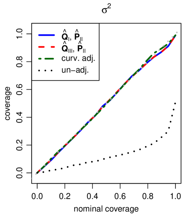
Figure 2: Empirical coverage rates for equi-tailed credible intervals based on MCMC samples using the tapered likelihood. Blue and red curves are OFS-adjusted samples using different estimates of $\boldsymbol{\Omega}$, green curves are from a curvature-adjusted sampler, and dotted curves are un-adjusted samples.

Figure 2 shows that the un-adjusted MCMC samples (dotted curves) yield horrible coverage properties for both $\sigma^{2}$ and $c$. It is somewhat interesting that while the “naive” intervals severely under-cover $\sigma^{2}$, they severely over-cover $c$. We therefore see that a naive implementation results in being overly optimistic about estimates of $\sigma^{2}$ while being overly pessimistic about estimates of $c$. The OFS-adjusted intervals display much more accurate coverage, achieving nearly nominal rates, although for $c$, the asymptotic expression for $\hat{\mathbf{Q}}$ seems to produce intervals that are systematically slightly too short. The curvature-adjusted sampler results in simliar coverage.

To explore how the marginal OFS adjustment differs from the conditional adjustment in the Gibbs sampler setting, we simulate data from a spatial linear model, $Y(\mathbf{s})\sim\text{GP}(\mathbf{X}\boldsymbol{\beta},C(\boldsymbol{\theta});\mathbf{s})$. We set $\boldsymbol{\beta}=(-0.5,0,0.5)^{\prime}$ and use the same spatial design and covariance function as above. The design matrix $\mathbf{X}$ is a $1600\times 3$ matrix of standard normal deviates, and the prior distribution for $\boldsymbol{\beta}$ is a vague normal centered at zero. At each Gibbs iteration, $\boldsymbol{\theta}$ is updated using a Metropolis step using the tapered likelihood, and $\boldsymbol{\beta}$ is updated by drawing directly from its conditionally conjugate full conditional distribution. The sampler is first run without adjustment, and $\hat{\boldsymbol{\theta}}_{\text{QB}}$ and $\hat{\boldsymbol{\beta}}_{\text{QB}}$ are computed as the quasi-posterior means. The marginal OFS adjustment matrix is then computed using the analytical expression from Shaby and Ruppert (2012) by plugging in $\hat{\boldsymbol{\theta}}_{\text{QB}}$ and $\hat{\boldsymbol{\beta}}_{\text{QB}}$. Next, the Gibbs sampler is run a second time using the estimated marginal OFS matrix to adjust the sample from the full conditional distribution of $\boldsymbol{\theta}$ at each iteration. Finally, the Gibbs sampler is run a third time, this time estimating the conditional OFS adjustment matrix at each iteration by maximizing the tapered likelihood function and plugging the resultant parameter estimates into the asymptotic formula for $\hat{\boldsymbol{\Omega}}$.

Because the conditional OFS-adjusted Gibbs sampler is so computationally expensive, we simulate just a few datasets and report the output from one of them. Figures 3 and 3 compare the marginal adjusted quasi-posterior distributions for the two covariance parameters, generated with the marginal and conditional OFS adjustments. The qq-plot for $\sigma^{2}$ shows almost perfect agreement except for a handful of MCMC samples on the upper tail. For the $c$ parameter, the qq-plot shows that the marginal OFS adjustment produces a quasi-posterior that is the same shape as that of the conditional adjustment, but is slightly shifted to the right. Figure 3 shows contours of a kernel density estimate of the joint marginal ofs-adjusted quasi-posterior distribution of the two covariance parameters, with the marginal adjustment in black and the conditional adjustment in gray. The contours are very similar, with some small differences appearing on the right half of the $\sigma^{2}$-axis, indicating good agreement between the two bivariate distributions. The output from all the simulated datasets looked qualitatively similar, with no noticeable systematic differences between the two adjustments. The choice of adjustment had no discernible effect on the quasi-posterior distribution of $\boldsymbol{\beta}$.

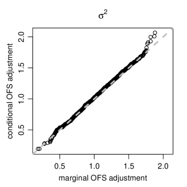
Figure 3: Comparison of marginal and conditional OFS-adjusted quasi-posterior distributions. Panels (a) and (b) show qq-plots of the marginal quasi-posteriors of the two covariance parameters. Panel (c) shows contour plots of a kernel density estimate of the joint quasi-posterior of the same parameters.

4.2 Composite likelihood for max-stable processes

Statistical models for extreme values that include spatial dependence are useful for studying, for example, extreme weather events like heat waves and powerful storms (Cooley et al., 2007; Sang and Gelfand, 2010, e.g.). Extreme value theory tells us that the distribution of block-wise maximum values (such as annual high temperatures) of independent draws from any distribution converges to a generalized extreme value (GEV) distribution (see Coles, 2001), if it converges at all. The asymptotics therefore suggest that any model of block-wise maxima at several spatial locations ought to have GEV marginal distributions with distribution function

$$F(y;\mu,\sigma,\xi)=\exp\Big{\{}-\Big{[}1+\xi\Big{(}\frac{x-\mu}{\sigma}\Big{)}\Big{]}^{-1/\xi}\Big{\}},$$

where $\mu$ is a location, $\sigma$ a scale, and $\xi$ a shape parameter that determines the thickness of the right tail. The GEV may be characterized by the max-stability property (Coles, 2001). More generally, block-wise maxima of random vectors must also converge to max-stable distributions.

Sang and Gelfand (2010) achieve spatial dependence with GEV marginals through a Gaussian copula construction. However, Gaussian copula models have been strongly criticized (Klüppelberg and Rootzén, 2006) because they do not result in max-stable finite-dimensional distributions, nor do they permit dependence in the most extreme values, referred to as tail dependence, and it is clear that physical phenomena of interest do exhibit strong spatial dependence even among the most extreme events.

An alternate approach for encoding spatial dependence of extreme values is through max-stable process models (de Haan, 1984), which are stochastic processes over some index set where all finite-dimensional distributions are max-stable. Explicit specifications of spatial max-stable processes based on the de Haan (1984) spectral representation have been proposed by Smith (1990), Schlather (2002), and Kabluchko et al. (2009). These formulations have the advantage that they do represent tail dependence.

Unfortunately, for all of the available spatial max-stable process models, joint density functions of observations at three or more spatial locations are not known (a slight exception is the Gaussian extreme value process (GEVP) (Smith, 1990), for which Genton et al. (2011) derives trivariate densities). Since bivariate densities are known, Padoan et al. (2010) proposes parameter estimation and inference via the pairwise likelihood, where all bivariate log likelihoods are summed as though they were independent:

$$\ell_{p}(\boldsymbol{\theta};\mathbf{y})=\sum_{i\neq j}\ell(y_{i},y_{j};\boldsymbol{\theta}).$$

The pairwise likelihood is a special case of a composite likelihood (Lindsay, 1988). Padoan et al. (2010) show that asymptotic normality of the form (2) applies, so we may again apply the OFS adjustment.

Our simulation experiment consists of 1000 draws from a GEVP with unit Fréchet margins on a $10\times 10$ square grid, with 100 replicates per draw. An example of a single replicate is shown in Figure 4. This setup would correspond, for example, to 100 years of annual maximum temperature data from 100 weather stations.

Figure 4: A realization of the Gaussian extreme value max-stable process of Smith (1990).

The unknown parameter $\boldsymbol{\theta}$ in a 2-dimensional GEVP is a $2\times 2$ covariance matrix. For this simulation, $\boldsymbol{\theta}_{0}=(\Sigma_{11},\Sigma_{12},\Sigma_{22})^{\prime}=(0.75,-0.5,1.25)^{\prime}$. The prior distribution for $\boldsymbol{\Sigma}$ is a vague inverse-Wishart. For each draw, a long MCMC chain is run and $\hat{\boldsymbol{\theta}}$ is computed as the posterior mean. In addition, for each draw, all four $\mathbf{Q-P}$ combinations of $\hat{\mathbf{Q}}_{\text{I}},\hat{\mathbf{Q}}_{\text{II}},\hat{\mathbf{P}}_{\text{I}}$, and $\hat{\mathbf{P}}_{\text{boot}}$, as defined above, are computed to produce four estimates of $\boldsymbol{\Omega}$. Finally, the curvature-adjusted MCMC sampler from Cooley et al. (2012) is run on each simulated dataset, with $\boldsymbol{\Omega}$ estimated from $\hat{\mathbf{Q}}_{\text{II}}$ and $\hat{\mathbf{P}}_{\text{I}}$, evaluated at the maximum pairwise likelihood estimate of $\boldsymbol{\Sigma}$.

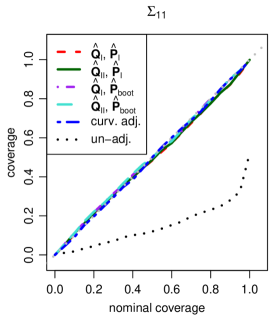
Figure 5: Empirical coverage rates for equi-tailed credible intervals based on MCMC samples using the pairwise likelihood. Colored curves are OFS-adjusted samples using different estimates of $\boldsymbol{\Omega}$, and from a curvature-adjusted sampler. Dotted curves are un-adjusted samples.

Figure 5 shows that, for this simulation, the OFS adjustment produces credible intervals that cover at almost exactly their nominal rates. Furthermore, OFS-adjusted credible intervals based on the four values of $\hat{\boldsymbol{\Omega}}$ turned out nearly identical. This is about as good a result as one could hope for. The curvature-adjusted sampler also achieves nominal coverage. The un-adjusted intervals systematically under-cover for each of the three parameters. This is expected (as noted by Cooley et al. (2012)), as the pairwise likelihood over-uses the data by including each location in roughly $n/2$ terms of the objective function rather than just one, as would be the case with a likelihood function. This results in a pairwise likelihood surface that is far too sharply-peaked relative to a likelihood surface. The OFS adjustment seems to successfully compensate for this effect.

5 Data analysis

5.1 Bird Counts

Next, we apply tapered quasi-Bayesian analysis to a hierarchical model that includes a Gaussian process. Instead of a purely spatial random field as in Section 4.1, we assume a spatio-temporal random field, which highlights some of the advantages of tapering over other methods designed for large spatial datasets.

The dataset comes from a “citizen science” initiative called eBird (www.ebird.org). The idea of citizen science is that many non-professional observers can be leveraged to collect an enormous amount of data. eBird participants across North Americal record the birds they see, along with the time and location of the observation, into a web-based database. Here, we look at 6114 observations of the Northern Cardinal in a section of the eastern United States over a period from 2004 to 2007 (Figure 1).

Inspection of the data suggests an overdispersed Poisson model. Let $Y_{i},\ldots,Y_{n}$ be observed counts and $\mathbf{X=[x}_{1},\ldots,\mathbf{x}_{n}]$ be a matrix of covariates associated with each observation. Also, let $\mathbf{S=[s}_{1},\ldots,\mathbf{s}_{n}]$ and $\mathbf{T=[t}_{1},\ldots,\mathbf{t}_{n}]$ be the spatial and temporal locations, respectively, associated with $Y_{i},\ldots,Y_{n}$, with space indexed by latitude and longitude.

For this example, we deliberately chose a small number of predictors, several of which vary spatially. Preliminary analyses led to a set of 10 covariates that includes time of day, day of year, human population density, percentage of developed open space (single-family houses, parks, golf courses, etc.), tree canopy density, and variables that measure observer effort. Simple transformations (logs, powers, etc.) were applied to some of the covariates, as suggested by ornithologists and exploratory analyses.

We specify the model as

$$y_{i}|\lambda_{i} \sim \mbox{Pois}(\lambda_{i})$$

$$\log{\lambda_{i}}(\mathbf{x}_{i},\mathbf{s}_{i},\mathbf{t}_{i}) = \mathbf{x}^{\prime}_{i}\boldsymbol{\beta}+Z_{i}(\mathbf{s}_{i},\mathbf{t}_{i})+\varepsilon_{i}$$

$$\mathbf{z}(\mathbf{S,T})|\boldsymbol{\theta}^{*} \sim N(0,\boldsymbol{\Sigma}^{*}(\boldsymbol{\theta}^{*};\mathbf{S,T}))$$

$$\varepsilon_{i}|\tau \sim \mbox{iid }N(0,\sigma^{2}_{\varepsilon}).$$ (10)

We assume that the random effect $\mathbf{z(S,T)}$ has a Gaussian random field structure. Thus, this model is an example of “model-based geostatistics” of Diggle et al. (1998), a class of spatial generalized linear models that has seen wide application in the environmental literature.

Even though Northern Cardinals are not migratory birds, a spatio-temporal structure for the random effect has a great intuitive appeal. One can easily imagine clusters of birds habiting different locales, moving from place to place based on things like food availability or disturbances. The correlation range of the spatio-temporal random effect informs the ornithologists about the scales of movements of Northern Cardinals in space and time, as well as providing clues about what un-measured covariates are needed to explain the pattern of Northern Cardinal observations.

The parameter $\boldsymbol{\varepsilon}$ can be interpreted as either an overdispersion parameter, or as the traditional “nugget” effect, representing small-scale variation or measurement error. It will be convenient to marginalize over the random effects $\mathbf{z}$ and $\boldsymbol{\varepsilon}$ and consider the distribution of the log-means directly. Furthermore, we will write the matrix $\boldsymbol{\Sigma}^{*}(\boldsymbol{\theta}^{*};\mathbf{S,T})+\sigma^{2}_{\varepsilon}\mathbf{I}$ simply as $\boldsymbol{\Sigma}(\boldsymbol{\theta};\mathbf{S,T})$ and condense $\boldsymbol{\theta}^{*}$ and $\sigma^{2}_{\varepsilon}$ into the single parameter vector $\boldsymbol{\theta}$. The resulting model, equivalent to (10), is written as

$$y_{i}|\lambda_{i} \sim \mbox{Pois}(\lambda_{i})$$

$$\log{\lambda_{i}}(\mathbf{x}_{i},\mathbf{s}_{i},\mathbf{t}_{i}) \equiv b_{i}$$

$$\mathbf{b}(\mathbf{X},\mathbf{S,T})|\boldsymbol{\theta},\boldsymbol{\beta} \sim N(\mathbf{X}\boldsymbol{\beta},\boldsymbol{\Sigma}(\boldsymbol{\theta};\mathbf{S,T})).$$ (11)

Another level in the hierarchy imposes a ridge penalty on the regression coefficients $\boldsymbol{\beta}$, specified as

$$\boldsymbol{\beta}\sim N(0,\sigma^{2}_{\beta}\mathbf{I}).$$ (12)

Finally, we need priors for the parameters $\boldsymbol{\theta}$ and $\sigma^{2}_{\beta}$

$$\theta_{i} \sim \pi_{\theta_{i}}$$

$$\sigma^{2}_{\beta} \sim \pi_{\sigma^{2}_{\beta}}$$

independently.

For $\boldsymbol{\Sigma}(\boldsymbol{\theta};\mathbf{S,T})$, we chose a spatio-temporal covariance model from Gneiting (2002). The covariance functions described therein are nonseparable in that (except in special cases) they cannot be written as the product of a purely spatial and purely temporal covariance function. Specifically, we let

$$C(\boldsymbol{\theta}^{*};\mathbf{h,u})=\frac{\sigma^{2}}{(a\mathbf{u}^{2\alpha}+1)^{2}}\cdot\exp{\bigg{\{}\frac{-(c/\sigma^{2})\mathbf{h}^{2\gamma}}{(a\mathbf{u}^{2\alpha}+1)^{\omega\gamma}}\bigg{\}}},$$ (13)

where $\mathbf{h}$ and $\mathbf{u}$ are distances between observation points in space and time, respectively. The parameters $\alpha\in(0,1]$ and $\gamma\in(0,1]$ control the smoothness of the process. We fixed these parameters at convenient values of 1 and .5, respectively, because they were not well-identified by the data.

The parameter $\omega\in[0,1]$ has the nice interpretation of specifying the degree of nonseparability between purely spatial and purely temporal components; when $\omega=0$, $C(\boldsymbol{\theta};\mathbf{h,u})$ is the product of a purely temporal and a purely spatial (exponential) covariance function.

Priors for the parameters $\sigma^{2}$, $a$, $c$, $\sigma^{2}_{\varepsilon}$, and $\sigma^{2}_{\beta}$ are specified as vague Cauchy distributions, truncated to have only positive support. The interaction parameter $\omega$ is given a uniform prior on $[0,1]$.

A valid spatio-temporal taper matrix may be constructed as the element-wise product of a spatial and a temporal taper matrix

$$\mathbf{T}=\mathbf{T}_{s}\circ\mathbf{T}_{t}.$$

Constructed this way, $\mathbf{T}$ inherits the sparse entries of both $\mathbf{T}_{s}$ and $\mathbf{T}_{t}$, and may therefore itself be extremely sparse.

Several other methods exist to mitigate the computational burden imposed by large spatial datasets with non-Gaussian responses. Wikle (2002) and Royle and Wikle (2005) embed a continuous spatial process into a latent grid and work in the spectral domain using fast Fourier methods. However, applying Fourier methods here is problematic, as it is not obvious how to do so for a process that has spatio-temporal structures. Low rank methods like predictive processes (Banerjee et al., 2008; Finley et al., 2009) and fixed rank Kriging (Cressie and Johannesson, 2008) are also popular for spatial data. Applying these methods to spatio-temporal models is possible, but awkward. For predictive processes, one must decide how to specify knot locations in space $\times$ time. For fixed rank Kriging, one must specify knot locations as well as space-time kernel functions. Fixed rank Kriging as been adapted to the spatio-temporal setting (Cressie et al., 2010) through a linear filtering framework, but only for Gaussian responses. Finally, Gauss-Markov approximations to continuous spatial processes are fast to compute, especially when using Laplace approximations in place of MCMC (Lindgren et al., 2011; Rue et al., 2009). However, again, these methods do not apply to data with spatio-temporal random effects.

In contrast, application of the tapering approach in the spatio-temporal context is immediate and even potentially enjoys increased computational efficiency relative to the purely spatial context because of the additional sparsity induced by element-wise multiplication with the temporal taper matrix.

For the eBird data, a taper range of 20 miles and 60 days gives a tapered covariance matrix with about .5% nonzero elements. MCMC was carried out using a block Gibbs sampler. Each evaluation of the expensive normal log likelihood was replaced by its tapered analogue. Within each Gibbs iteration, each of $\mathbf{b}$, $\boldsymbol{\theta}$, and $\sigma^{2}_{\beta}$ are updated with a random walk Metropolis step. The full conditional distribution for $\boldsymbol{\beta}$ is conditionally conjugate, enabling a simple update as a draw from the appropriate normal distribution.

As described in Section 3.3, the tapered Gibbs sampler was run twice. Samples from the first run were used to produce point estimates of $\boldsymbol{\theta}$ and the marginal OFS adjustment matrix $\boldsymbol{\Omega}_{\boldsymbol{\theta}|\boldsymbol{\beta},\mathbf{b},\sigma^{2}_{\beta}}$. The estimate $\hat{\boldsymbol{\Omega}}_{\boldsymbol{\theta}|\boldsymbol{\beta},\mathbf{b},\sigma^{2}_{\beta}}$ was computed from the asymptotic expressions for $\mathbf{Q}$ and $\mathbf{Q}$ evaluated at $\hat{\boldsymbol{\theta}}_{\text{QB}}$, the quasi-posterior mean. Because the quasi-posterior distribution of interaction parameter $\omega$ was nearly uniform on [0,1], it was excluded from the adjustment. The conditional OFS was not attempted, as doing so would have required several months of computation time.

After discarding 5000 burn-in iterations, 5000 MCMC samples were used for estimation and prediction. Pointwise quantiles of the posterior correlation surface are shown in Figure 6, for both the un-adjusted and adjusted samples. The point at which the correlation drops to .05, often called the “effective range” of a process, is the most extreme contour displayed in each of the plots in figure 6. While the two sets of contours do not differ much in the median, they are quite different in the upper and lower quantiles. For this analysis, the correlation structure is a key component with a useful interpretation, so its posterior uncertainty is of interest. Comparing the OFS-adjusted and un-adjusted correlation surfaces, it is interesting to note that OFS adjustment gives decreased temporal uncertainty but increased spatial uncertainty.

The fairly long median effective range of around 225 days at spatial lag 0 seemed reasonable to a panel of ornithologists, as Northern Cardinals, while they do move around to some degree, are not migratory birds. The effective range of 3 miles at time lag 0 seemed reasonable as well. Northern Cardinals build new nests each year and are socially monogamous within a breeding season, but divorces sometimes occur between years. They generally stay close to the nest to forage and bathe. Males are highly territorial and will occasionally challenge neighboring males’ breeding territories. These behaviors are consistent with a the posterior median temporal dependence range of a significant fraction of a single year, and a posterior median spatial range that is larger than but in the ballpark of an individual’s territorial range.

Figure 6: Posterior quantiles of spatio-temporal correlation surface. The top row was computed from the un-adjusted sampler, and the bottom row was computed from the OFS-adjusted sampler. The median surfaces are similar, but the high and low quantile contours show that the uncertainty is noticeably altered by the adjustment.

Posterior estimates for some of the more interesting fixed effects, along with 95% pointwise credible intervals, are plotted in Figure 7. The top right panel shows a clearly increasing trend as a function of the number of hours spent observing. The top right panel shows that the effect as a function of time of day increases until about 8 a.m. and then decreases until about 3 p.m., when it again begins to increase. The increase after 3 p.m. is accompanied by very wide credible intervals. In the bottom left panel, we can see an overwhelming negative effect at high elevations. Finally, the bottom right panel shows a seasonal cycle that peaks in early winter and attains its minimum in later summer.

Figure 7: A subset of the estimated fixed effects. Solid lines are posterior medians, and shaded areas are posterior pointwise 90% credible intervals.

Recall that these fixed effects are on the log scale. Here again, a panel of ornithologists was pleased with the results. Obviously, the number of observed counts should increase with the amount of time an observer spends watching. The peak in the time of day effect at around 8 a.m. reflects the time of the highest activity level of the birds. The wide confidence bands starting at around 4 p.m. probably results from a lack of data in the afternoon. Northern Cardinals cannot live in habitats found at higher elevations, a fact reflected in the huge negative effect estimated after about 700 meters. Finally, cardinals tend to be easier to detect during the winter months because they are more vocal, and they visit feeders more frequently. In the summer months, they tend to stay more hidden because it is their breeding season, and they do not visit feeders as often because food is more plentiful. These seasonal variations in detectability are reflected in the pattern shown in the estimated date effect.

The median posterior predicted surface (Figure 8) of the mean counts was generated by drawing from the posterior predictive distribution at a large set of sample points in the spatial domain, for fixed values of “effort” covariates, and at a fixed time.

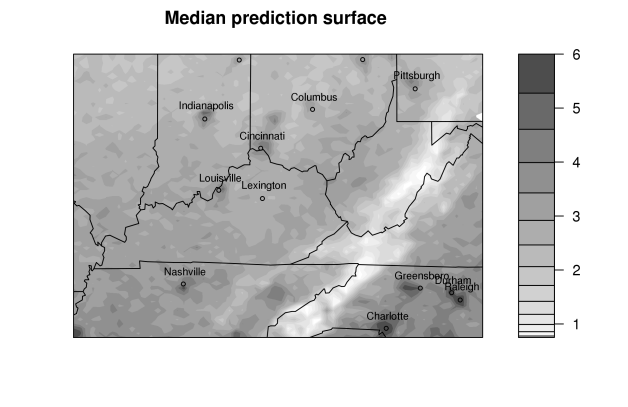
Figure 8: Median predicted surface for 8 a.m. on April 11.

Maps like Figure 8, of course, vary in time as well as space. The most prominent feature of the predicted surface is the very low values along the Appalachians. This is a result of the huge elevation effect, and corroborates expert knowledge. Another noticeable feature of the prediction surface is the elevated counts around population centers. It is well-known among ornithologists that Northern Cardinals are most common in the suburbs. This happens for two reasons. The first is that they are attracted to the many bird feeders found in the suburbs. The second is that suburban habitat, with landscaped gardens and mixes of open areas, shrubs, and trees, is ideal habitat for cardinals.

6 Discussion

The open-faced sandwich adjustment provides a way to incorporate estimating functions that are not likelihoods into Bayesian-like models. While the resulting inference does not enjoy the elegant formal probabilistic interpretation of pure Bayesian analysis, it does inherit some of its most desirable attributes: borrowing strength across parameters, the ability to work with complicated hierarchical structures, and propagating uncertainty throughout model components, to name a few. When the likelihood function is unknown or has undesirable properties, the OFS adjustment allows one to retain these beneficial features of Bayesian analysis while avoiding the need to compute the likelihood function by substituting a suitable objective function in its place.

These benefits come with a few costs. First, the resultant MCMC samples may not be interpreted as though they came from a true Bayesian model. Second, the coverage characteristics of the output are only as good as the applicability of the asymptotic approximation and the practitioner’s ability to estimate the sandwich matrix, which can be a difficult task in some situations (Kauermann and Carroll, 2001). Third, estimating the adjustment matrix using sample moments or a bootstrap and relying on it to produce posterior samples has a decidedly “un-Bayesian” feel to it. Finally, using the adjustment in the Gibbs sampler context does require approximately twice the computational effort as the un-adjusted Gibbs sampler, which in some cases can be considerable.

In addition to these considerations, comparisons between the OFS adjustment and the curvature adjustment of Cooley et al. (2012) seem natural. In our simulations, both adjustments performed extremely well. The curvature adjustment shares with OFS both the advantages and disadvantages described above. But in addition, the curvature adjustment, as implemented in the data example in Cooley et al. (2012), has several additional drawbacks to consider. First, Cooley et al. (2012) require an outside method to estimate of $\boldsymbol{\theta}$ and $\boldsymbol{\Omega}$, whereas the OFS adjustment uses the MCMC sample to estimate $\boldsymbol{\theta}$ and $\boldsymbol{\Omega}$. Using the un-adjusted quasi-posterior sample to estimate $\boldsymbol{\theta}$ and $\boldsymbol{\Omega}$ as we do here takes advantage of borrowing strength, leveraging prior information, etc. that simply maximizing $\ell_{M}(\boldsymbol{\theta})$ cannot. We note, however, that this drawback in the curvature adjustment can easily be avoided. One could easily apply the strategy that we suggest in Section 3.3, running the sampler first without adjustment to estimate $\boldsymbol{\theta}$ and $\boldsymbol{\Omega}$ in a Bayesian-like way, and then using these estimates to implement the curvature-adjusted sampler. In the Metropolis context, this strategy requires twice the computational effort of OFS; since OFS is applied to the sample post hoc, there is no need to run the sampler a second time. In the Gibbs sampler setting, however, the computational burden is identical.

More obvious is the enormous computational cost imposed by estimating the conditional adjustment matrix in the adaptive version of the curvature adjusted Gibbs sampler favored by Cooley et al. (2012). This simply would not have been feasible, for example, in the eBird example of Section 5.1. We note that this complication can probably be avoided by using the marginal, rather than the conditional, version of $\hat{\boldsymbol{\Omega}}$. In fact, since their simulated comparisons between the marginal and conditional forms of $\hat{\boldsymbol{\Omega}}$ performed so similarly, we are confused as to why Cooley et al. (2012) use the much more computationally expensive conditional version in their data example. In the end, conditional on implementation details, the OFS and curvature adjustments are quite similar both in performance and in spirit.

References

- Banerjee et al. (2004) Sudipto Banerjee, Bradley P. Carlin, and Alan E. Gelfand. Hierarchical Modeling and Analysis for Spatial Data. Monographs on Statistics and Applied Probability. Chapman & Hall/CRC, Boca Raton, 2004.
- Banerjee et al. (2008) Sudipto Banerjee, Alan E. Gelfand, Andrew O. Finley, and Huiyan Sang. Gaussian predictive process models for large spatial data sets. J. R. Stat. Soc. Ser. B Stat. Methodol., 70(4):825–848, 2008.
- Bayarri and Berger (2004) M.J. Bayarri and J.O. Berger. The interplay of Bayesian and frequentist analysis. Statistical Science, 19(1):58–80, 2004.
- Berger et al. (2001) James O. Berger, Victor De Oliveira, and Bruno Sansó. Objective Bayesian analysis of spatially correlated data. J. Amer. Statist. Assoc., 96(456):1361–1375, 2001.
- Bhapkar (1972) V. P. Bhapkar. On a measure of efficiency of an estimating equation. Sankhyā Ser. A, 34:467–472, 1972. ISSN 0581-572X.