Constraints on Superconducting Cosmic Strings from Early Reionization

Abstract

Electromagnetic radiation from superconducting cosmic string loops can reionize neutral hydrogen in the universe at very early epochs, and affect the cosmic microwave background (CMB) temperature and polarization correlation functions at large angular scales. We constrain the string tension and current using WMAP7 data, and compare with earlier constraints that employed CMB spectral distortions. Over a wide range of string tensions, the current on the string has to be less than $\sim 10^{7}~{}{\rm GeV}$.

I Introduction

Spontaneous breaking of symmetries in unified theories of particle physics can lead to the formation of cosmic strings (for a review see, e.g., LindeBook ; VilenkinBook ; Copeland09 ; Copeland11 ). In certain models, the cosmic strings can be superconducting Witten:1984eb .

As superconducting cosmic strings pass through magnetized regions, they accumulate electric currents, and emit electromagnetic radiation Vilenkin:1986zz and particles Witten:1984eb ; Berezinsky:2009xf . Therefore, the presence of currents on strings leads to a number of observational signatures that can be probed by present and future experiments. Radiation from strings is not isotropic but is most efficient at cusps — parts of a string that move very close to the speed of light — and kinks — discontinuities in the tangent vector to the string. The strongly beamed radiation has been studied as sources of various observable effects such as gamma ray bursts Paczynski ; Berezinsky:2001cp , ultra high energy neutrinos Berezinsky:2009xf , radio transients Vachaspati:2008su ; Cai:2011bi , and distortions of the cosmic microwave background (CMB) Tashiro:2012nb ; Sanchez89 ; Sanchez90 . In addition to these signatures that are particular to superconducting strings, there are more generic effects that are gravitational and do not rely on superconductivity. These include the anisotropy of the CMB temperature Dvorkin11 and B-mode plarization Pogosian08 ; Avgoustidis:2011ax , gravitational waves Damour01 ; Damour05 ; pulsar ; Olmez ; Battye ; Dufaux12 , gravitational lensing lensing , wakes in the 21cm maps Brandenberger:2010hn ; Hernandez:2011ym ; McDonough:2011er ; Hernandez:2012qs ; Pagano:2012cx , early structure formation Shlaer:2012rj , early reionization due to early structure formation Olum:2006at , and formation of dark matter clumps Berezinsky:2011wf .

In this paper, we focus on the reionization of cosmic hydrogen gas in the intergalactic medium (IGM) due to photons emitted from superconducting cosmic string loops. Hydrogen gas in the IGM was electrically neutral after cosmic recombination, which occurs at a redshift $z_{\rm rec}\approx 1100$. However, as luminous structures, such as stars and galaxies form, ultra-violet (UV) photons emitted by these objects ionize surrounding hydrogen gas. Finally, hydrogen gas in the IGM is totally “reionized” Barkana:2000fd . The observation of the Gunn-Peterson effect Gunn & Peterson (1965) in high redshift quasar spectra, which probes the amount of neutral hydrogen along the line of sight, suggests that full reionization was accomplished by $z\sim 6$ Fan:2005es . Recently, WMAP measured the CMB anisotropy, and obtained the optical depth due to Thomson scattering, $\tau\sim 0.088$, in WMAP 7-year data Komatsu:2010fb . This result implies that the cosmological reionization process began around $z=10$, at least.

In contrast to UV emission due to structure formation, superconducting cosmic string loops emit ionizing photons even at high redshifts, $z>100$, when there are a few luminous objects which can ionize hydrogen. Therefore, the existence of superconducting cosmic strings can cause early reionization. Once early reionization occurs, it leaves footprints on the CMB temperature and polarization anisotropy spectra. By using Markov Chain Monte Carlo (MCMC) analysis, and taking into account the effect of superconducting cosmic string loops, we evaluate the CMB anisotropy spectra, and compare them with WMAP 7-year data.

This paper is organized as follows. We calculate the radiation emitted by superconducting cosmic string loops in Sec. II.1, and in Sec. II.2 we find the ionization fraction due to UV photons emitted by cosmic string loops. In Sec. II.2, we also calculate the optical depth for Thomson scattering of CMB photons on free electrons, and compare the ionization history with strings to the standard history without strings used by WMAP analysis. In Sec. III, we estimate the effects of string loops on CMB anisotropies. In conclusion, we obtain constraints on the string tension, $G\mu$, and the electric current, $I$, on the string in Sec. IV.

Throughout this paper, we use parameters for a flat $\Lambda$CDM model: $h=0.7$ $(H_{0}=h\times 100~{}{\rm km/s/Mpc})$, $\Omega_{b}=0.05$ and $\Omega_{m}=0.26$. Note also that $1+z=\sqrt{t^{\prime}/t}$ in the radiation dominated epoch, and $1+z=(1+z_{\rm eq})(t_{\rm eq}/t)^{2/3}$ in the matter dominant epoch, where $t^{\prime}=(2\sqrt{\Omega_{r}}H_{0})^{-1}$ and $z_{\rm eq}=\Omega_{m}/\Omega_{r}$ with $h^{2}\Omega_{r}=4.18\times 10^{-5}$. We also adopt natural units, $\hbar=c=1$.

II Reionization from Cosmic String Loops

II.1 UV Photon Emission from Loops

Solutions to the dynamical equations for cosmic strings show that a cosmic string loop often develops cusps and almost always has kinks. These features lead to the emission of high energy photons from superconducting cosmic strings. The number of photons emitted from a cusp per unit time per unit frequency is Cai:2011bi

$$f_{\omega}^{c}\equiv\frac{d^{2}N_{c}}{d\omega dt}\sim\frac{4\pi}{3}\frac{I^{2}L^{1/3}}{\omega^{5/3}},$$ (1)

and from a kink radiokink

$$f_{\omega}^{k}\equiv\frac{d^{2}N_{k}}{d\omega dt}\sim 2\pi\psi\frac{I^{2}}{\omega^{2}},$$ (2)

where $I$ is the current, $L$ is the loop length, $\psi$ is the sharpness of the kink, and $\omega$ is the frequency of the emitted photon.

Note that the radiated electromagnetic power from a single cusp dominates over the power radiated from a single kink by a factor $\sim(\omega L)^{1/3}\gg 1$, since the loop length is much larger than the radiation wavelength of interest.

The spectrum of photons emitted from cosmic string loops per unit physical volume is

$$\frac{d^{2}\mathcal{N}}{d\omega dt}=\int dn(L,t)\frac{d^{2}N}{d\omega dt},$$ (3)

where $dn(L,t)$ is the number density of loops in the matter dominated era

$$dn(L,t)=\frac{\kappa C_{L}dL}{t^{2}(L+\Gamma G\mu t)^{2}}\ ,\ \ t>t_{\rm eq},$$ (4)

where $\kappa\sim 1$, and $C_{L}\equiv 1+\sqrt{t_{\rm eq}/(L+\Gamma G\mu t)}$. The second term in $C_{L}$ accounts for loops in the matter dominated era that are left over from the radiation dominated era. We note that the distribution of cosmic string loops is not completely established. Although analytical studies Rocha:2007ni ; Polchinski07 ; Dubath08 ; Vanchurin11 ; Lorenz:2010sm and cosmic string network simulations Bennett90 ; Allen90 ; Hindmarsh97 ; Martins06 ; Ringeval07 ; Vanchurin06 ; Olum07 ; Shlaer10 ; Shlaer11 agree on the distribution of large loops, there is disagreement on the distribution of small loops. We have checked that a different choice of loop distribution, e.g., as suggested in Ref. Lorenz:2010sm , does not change our final constraints significantly.

Then, the number of photons emitted from all cusps per unit time per unit volume per unit frequency is given by

$${d^{2}\mathcal{N}_{c}\over d\omega dt}\approx{8\pi\kappa{\cal C}\over 9}\left(t_{eq}\over t\right)^{1/2}{I^{2}\over(\Gamma G\mu)^{7/6}t^{8/3}}\,\omega^{-5/3},$$ (5)

in the matter dominated epoch, where $\Gamma$ is determined by the dominant energy loss mechanism, as discussed below Eq. (8), and ${\cal C}$ is the average number of cusps per loop. The number of kinks per loop is expected to be quite large, and the radiation will also depend on the sharpness of the kinks $\psi$. The effective number of kinks per loop, i.e., weighting a kink by its sharpness, will be denoted by ${\cal K}$, and then, the number of photons emitted per unit time per unit volume per unit frequency from kinks is

$$\frac{d^{2}\mathcal{N}_{k}}{d\omega dt}\approx\frac{4\pi\kappa{\cal K}}{3}\left(t_{eq}\over t\right)^{1/2}\frac{I^{2}}{(\Gamma G\mu)^{3/2}t^{3}}\,\omega^{-2}.$$ (6)

Unless ${\cal K}$ is larger than ${\cal C}(\omega\Gamma G\mu t)^{1/3}$, the number of photons emitted by cusps is larger than the number emitted by kinks. We shall assume that cusps dominate the emission from string loops.

Cosmic string loops also emit gravitational waves with power VilenkinBook

$$P_{g}\sim\Gamma_{g}G\mu^{2},$$ (7)

where $\Gamma_{g}\sim 50$, whereas the power due to electromagnetic radiation from superconducting loop cusps is VilenkinBook

$$P_{\gamma}\sim\Gamma_{\gamma}I\sqrt{\mu},$$ (8)

where $\Gamma_{\gamma}\sim 10$. $P_{g}\sim P_{\gamma}$ at the critical value of the current

$$I_{*}\equiv\frac{\Gamma_{g}G\mu^{3/2}}{\Gamma_{\gamma}}.$$ (9)

The lifetime of a loop is determined by the dominant energy loss mechanism, and can be estimated as

$$\tau=\frac{\mu L}{P}\equiv\frac{L}{\Gamma G\mu},$$ (10)

where

$$\Gamma\approx \Gamma_{g} I<I_{*}$$   for (11)

$$\Gamma\approx \Gamma_{g}\frac{I}{I_{*}} I>I_{*}$$   for . (12)

II.2 Ionization Fraction

UV photons emitted from a loop of cosmic string ionize hydrogen in the surrounding medium since the mean free path of UV photons is very short. If we assume that one emitted ionizing photon ionizes one hydrogen atom, then the ionization rate in the region surrounding a loop is equal to the number of ionizing photons emitted from the loop per unit time

$${dN_{i}\over dt}=\int_{\omega_{i}}^{\omega_{c}}d\omega~{}f_{\omega},$$ (13)

where $f_{\omega}$ is the spectrum of the photons emitted from a loop of cosmic string given by Eq. (1), and the integration is from the Lyman $\alpha$ frequency, $\omega_{i}=13.6~{}$eV, to a high frequency cutoff, $\omega_{c}$. Photons with energy higher than $\omega_{c}$ do not contribute to the photo–ionization, because the cross-section decreases rapidly as the photon energy increases Zdziarski89 . Since the number of ionizing photons falls off with frequency, our results are not very sensitive to the exact value of $\omega_{c}$, and we will set $\omega_{c}=10^{4}~{}$eV.

The recombination rate in the volume surrounding the loop is

$${dn_{r}\over dt}=n_{e}n_{\rm HII}\alpha_{r}=n_{\rm H}^{2}\alpha_{r},$$ (14)

where $\alpha_{r}$ is the recombination coefficient. Typically $\alpha_{r}=2.6\times 10^{-13}\,{\rm cm}^{3}/{\rm s}$ at $T_{e}=10^{4}~{}$K, and $n_{\rm H}=8.42\times 10^{-6}\,(1+z)^{3}\,\Omega_{B}h^{2}~{}{\rm cm}^{-3}$. In order to get the final expression in Eq. (14), we assume that all the hydrogen inside the surrounding volume is ionized, i.e., $n_{\rm HII}=n_{e}=n_{\rm{H}}$.

The steady-state assumption between the ionization and recombination rates in the surrounding region allows us to determine the ionized volume around a loop of length $L$,

$$V(L)={dN_{i}/dt\over dn_{r}/dt},$$ (15)

where the numerator is given in Eq. (13), and the denominator in Eq. (14). This is the volume around a single loop and depends on the length, $L$, of the loop. We can obtain the ionization fraction due to all cosmic string loops, $x_{\rm s}$, by multiplying the number density of loops, $dn(L,t)$, by $V(L)$, and integrating over $L$,

$$x_{\rm s} = \int dn(L,t)V(L)$$ (16)

$$= {1\over n_{\rm H}^{2}\alpha}\int_{\omega_{i}}^{\omega_{c}}d\omega\int dn(L,t)f_{\omega}(L,t)$$

$$\equiv {1\over n_{\rm H}^{2}\alpha}\int_{\omega_{i}}^{\omega_{c}}d\omega\frac{d^{2}\mathcal{N}_{c}}{d\omega dt}.$$

Using Eq. (5), we can perform the integration to get

$$x_{\rm s}(z)={4\pi\kappa\over 3\alpha n_{H}^{2}(z)}\left(t_{eq}\over t\right)^{1/2}{{\cal S}\over t^{8/3}}\left(\omega_{i}^{-2/3}-\omega_{c}^{-2/3}\right),$$ (17)

where $z\sim z_{eq}(t/t_{eq})^{-2/3}$ in the matter dominated epoch and

$${\cal S}=\frac{I^{2}}{(\Gamma G\mu)^{7/6}}.$$ (18)

Note that the reionization signature from strings only depends on the particular combination of string tension and electric current that occurs in ${\cal S}$. Hence, observations will impose constraints on ${\cal S}$. In contrast to the standard scenario where structure formation suddenly results in reionization, cosmic strings cause early reionization that builds up gradually. From Eq. (17), we see that the ionization due to cosmic strings grows with decreasing redshift as

$$x_{\rm s}\propto z^{-5/4}\ ,\ \ z\gg 1\ .$$ (19)

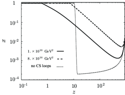
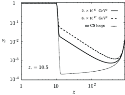
Figure 1: The dotted line shows the reionization fraction in the absence of cosmic strings, as modeled by WMAP. The solid and dashed curves in the top panel show the reionization fraction from cosmic strings, $x_{\rm s}(z)$, for two different values of the parameter ${\cal S}$ defined in Eq. (18). In the bottom panel we plot the total reionization fraction, $x(z)$, which is a sum of the structure formation, residual, and string components for a few different string parameters.

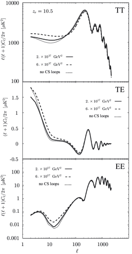
Figure 2: CMB anisotropy spectra with fixed $z_{r}=10.5$. The panels from top to bottom show $TT$, $TE$ and $EE$ angular spectra, respectively. The solid line is for cosmic string loops with ${\cal S}=2\times 10^{17}~{}{\rm GeV}^{2}$, for which the optical depth is $\tau=0.1$. The dashed line represents the case for ${\cal S}=6\times 10^{17}~{}{\rm GeV}^{2}$, for which the optical depth is $0.13$. For comparison, we plot the WMAP recommended reionization model (dotted curve) with the $\tanh$-shape reionization with $z_{r}=10.5$.

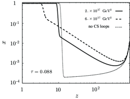
Figure 3: Possible reionization histories with fixed optical depth $\tau=0.09$, without strings (dotted) and with strings for two values of ${\cal S}$.

The reionization due to strings is in addition to the reionization due to structure formation. Hence, the total ionization fraction is

$$x=(x_{0}+x_{\rm res})+x_{\rm s},$$ (20)

where $x_{0}$ denotes the ionization fraction due to structure formation, and $x_{\rm res}$ the residual ionization from the epoch of recombination. The reionization fractions are functions of redshift, and the WMAP7 team has modeled $x_{0}(z)$ as

$$x_{0}(z)=\frac{1}{2}\left[1+{\rm tanh}\left(\frac{2(1+z_{r})^{3/2}-(1+z)^{3/2}}{3\Delta z(1+z_{r})^{1/2}}\right)\right],$$ (21)

with $z_{r}\sim 10$ and $\Delta z\sim 0.5$. Note that the total ionization fraction cannot exceed unity. Our result in Eq. (17) however, can exceed 1 because we have assumed that the volumes reionized by different loops do not overlap. This assumption becomes invalid at high reionization fraction, and so $x$ is cutoff at 1 if Eq. (20) evaluates to a value larger than 1. In Fig. 1, we show $x_{0}+x_{\rm res}$ and $x_{\rm s}$, and also the total reionization fraction, $x$, as functions of $z$.

We can also calculate the optical depth for Thomson scattering as

$$\tau=\int_{t_{rec}}^{t_{0}}dt~{}n_{e}\sigma_{T},$$ (22)

where $t_{rec}$ is the time of recombination epoch, $t_{0}$ is the present age of the universe, $\sigma_{T}$ is Thomson scattering cross-section. The optical depth for the solid line in the top panel of Fig. 1 reaches $\tau\sim 0.09$, which is consistent with WMAP recommended value. However, the reionization by cosmic string loops is very slow. For comparison, we plot a $\tanh$-step ionization fraction parameterized by the middle point $z_{r}$ and duration $\Delta z$ as used by the WMAP 7-year analysis Komatsu:2010fb . This toy model in Fig. 1 gives the optical depth $\tau\sim 0.09$.

In the matter dominated epoch, the evolution of the ionization fraction due to cosmic string loops is given by Eq. (19). As a result, even at $z\sim 2$, the ionization fraction is less than 0.5 for ${\cal{S}}=10^{18}~{}{\rm GeV}^{2}$. This result conflicts with Gunn-Peterson test for high redshift quasars that the ionization fraction at $z\sim 6$ is larger than 0.9 Fan:2005es .

To satisfy the Gunn-Peterson test, at least ${\cal S}=8\times 10^{18}~{}{\rm GeV}^{2}$ is required as shown with the dashed line in the top panel of Fig. 1. However, the optical depth is $\tau\sim 0.7$ in this case. Thus, it is difficult to fit the CMB anisotropy spectrum in this model to the WMAP data, where we use cosmological parameters that are consistent with other cosmological observations. Therefore, we can conclude that the electromagnetic radiation from cosmic string loops is not a primary source for the cosmological reionization. A more consistent model with cosmic string loops, which satisfies the constraints of both the optical depth and Gunn-Peterson test, is the tanh-shape model with subdominant contribution of cosmic string loops. This leads to the reionization histories shown in the bottom panel of Fig. 1.

Before closing this section, we comment on the assumptions we made when evaluating the ionized volume $V$. We have ignored the velocities of cosmic string loops, and then evaluated the ionized volume $V$, assuming that a cosmic string loop ionizes the same region continuously. Since a cosmic string loop is expected to have relativistic center of mass velocity, the ionized region will continually shift with the motion of the cosmic string loop. However, we are interested in the average ionized fraction and the location of the ionized volume at any instant of time does not matter. Thus, we can neglect the velocity of cosmic string loops. Note that as cosmic strings move they also create wakes Shlaer:2012rj , and can lead to early structure formation Shlaer:2012rj , which can indirecly affect the reionization history Olum:2006at .

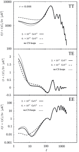
Figure 4: The CMB E-mode polarization anisotropy spectra with fixed optical depth $\tau=0.088$. The solid line is for cosmic string loops with ${\cal S}=2\times 10^{17}~{}{\rm GeV}^{2}$ and $z_{r}=9.1$. The dashed line is for ${\cal S}=6\times 10^{17}~{}{\rm GeV}^{2}$ and $z_{r}=3.5$. For comparison, we plot the case without cosmic string loops as the dotted line.

In the integration in Eq. (13), we have ignored photons with energy higher than $\omega_{c}=10^{4}~{}$eV since the universe is transparent to photons with higher energies. However, cosmological redshift can decrease the energies of such photons, and reduce them to below $\omega_{c}$. Even if we take this redshift effect into account, the optical depth of photo ionization is negligibly-small Zdziarski89 . Therefore, we can ignore photons with energy higher than $10^{4}~{}$eV since they do not contribute to the ionization process.

III Effect on CMB anisotropy

Reionization of the cosmic medium affects the CMB temperature and polarization correlators. Thus, CMB observations can lead to constraints on superconducting cosmic strings. We calculate CMB anisotropy with modified CAMB code Lewis:1999bs to take into account the effect of cosmic string loops on cosmic reionization.

We first fix the parameter $z_{r}=10.5$ in Eq. (21). As discussed above and shown in Fig. 1, this leads to different reionization histories with different optical depths. The results for the CMB correlators are shown in Fig. 2. The high optical depth due to cosmic string loops suppresses the amplitude of the acoustic oscillations in the temperature anisotropy as shown in the top panel of Fig. 2. The high optical depth enhances the amplitude on small $\ell$ in both the temperature and polarization anisotropy spectra, because Thomson scattering in the induced early reionization generate additional CMB anisotropy.

Next, we fix the optical depth to $\tau=0.088$, and let $z_{r}$ be an independent parameter. Since the optical depth is an integral over the ionization fraction, it depends on both $z_{r}$ and ${\cal S}$, and fixing $\tau$ leads to a relation between $z_{r}$ and ${\cal S}$. For example, $z_{r}=9.1$ for ${\cal S}=2\times 10^{17}$, and $z_{r}=3.5$ for ${\cal S}=6\times 10^{17}$. On the other hand, $\tau=0.088$ requires $z_{r}\sim 11$ without cosmic string loops. The redshift evolution of the ionization fraction for this case is shown in Fig. 3.

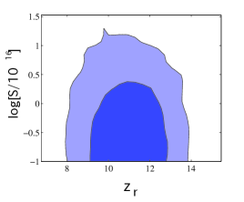
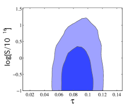
Figure 5: The 2-D contour of marginalized probabilities, in the ${\cal S}-z_{r}$ plane on the top, and the ${\cal S}-\tau$ plane on the bottom. The contours from the inside to the outside show the 1-sigma and 2-sigma confidence level.

The CMB anisotropy spectra are shown in Fig. 4. Larger values of ${\cal S}$ enhance the amplitude of CMB temperature anisotropy at large angular scales (small $\ell$). The peak position of $E$-mode polarization on small $\ell$ depends on the scale of the quadrupole component of CMB temperature anisotropy at the reionization epoch, $z_{r}$. Earlier reionization, corresponding to larger $\cal S$, implies that this peak occurs at lower $\ell$.

IV Conclusions

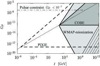
Figure 6: The reionization constraint on the $I$–$G\mu$ plane shown in conjunction with the CMB spectral distortion and other constraints. The lightly shaded region is ruled out from WMAP 7-year result. CMB $\mu$-distortion constraints by COBE-FIRAS measurement rule out the dark shaded area. The millisecond pulsar observations constrain $G\mu\lesssim 10^{-7}$ and is shown as the dot-dashed line. The region above the diagonal thin dashed line is where gravitational radiation dominates over electromagnetic radiation, i.e., $I<I_{*}$. Possible future constraints from CMB $\mu$-distortion are also shown by the dashed line if no such effect is seen by PIXIE. The hatched region is excluded because $I>\sqrt{\mu_{s}}$, and exceeds the saturation value of the current on superconducting strings.

In order to get the constraint on cosmic string loops from WMAP 7 year data, we take MCMC analysis in the $\Lambda$CDM flat universe model with modified COSMOMC code Lewis:2002ah to take into account the reionization effect of cosmic string loops. Fig. 5 shows 2-D contour of marginalized probabilities. Recall that $z_{r}$ is the redshift at which $\tanh$-shape reionization fraction is 0.5. From WMAP 7 year data, we obtain the constraint ${\cal S}<3\times 10^{16}~{}{\rm GeV}^{2}$ at the 1-$\sigma$ confidence level.

Accordingly, from Eq. (18), we obtain the constraint

$$G\mu\gtrsim 10^{-11}\left({10^{3}~{}{\rm GeV}\over I}\right)^{7/12},$$ (23)

for the gravitational radiation dominant case, $I<I_{*}$, and

$$G\mu\lesssim 4\times 10^{-13},$$ (24)

for the electromagnetic radiation dominant case, $I>I_{*}$.

We plot these constraints in the $I$–$G\mu$ plane in Fig. 6 as the lightly shaded region. For comparison we also show the constraint from $\mu$-distortion with COBE-FIRAS result as the dark shaded region, and possible future constraint from PIXIE where the interior region of the dashed triangle can be ruled out if no spectral distortion is observed by PIXIE, which was studied in Ref. Tashiro:2012nb .

Fig. 6 shows that reionization constraints on superconducting strings are much tighter than the constraints from CMB spectral distortions. In future, the PIXIE experiment to measure CMB spectral distortions at very low levels will be able to impose constraints that are stronger than current reionization constraints. Even then, reionization constraints will be stronger for light strings with large currents.

- (1) A.D. Linde, “Particle Physics and Inflationary Cosmology”, (CRC Press 1990).
- (2) A. Vilenkin and E.P.S. Shellard, “Cosmic Strings and Other Topological Defects”, Cambrigde University Press (1994).
- (3) E.J. Copeland and T.W.B. Kibble, “Cosmic Strings and Superstrings”, Proc. Roy. Soc. Lond. A 466, 623 (2010) [arXiv : hep-th/0911.1345].
- (4) E.J. Copeland, L. Pogosian and T. Vachaspati, “Seeing String Theory in the Cosmos”, Class. Quant. Grav. 28, 204009 (2011) [arXiv:1105.0207].
- (5) E. Witten,“Superconducting Strings,”, Nucl. Phys. B 249, 557 (1985).
- (6) A. Vilenkin and T. Vachaspati, “Electromagnetic Radiation from Superconducting Cosmic Strings,” Phys. Rev. Lett. 58, 1041 (1987).
- (7) V. Berezinsky, K.D. Olum, E. Sabancilar and A. Vilenkin, “UHE neutrinos from superconducting cosmic strings”, Phys. Rev. D 80, 023014 (2009) [arXiv:0901.0527].
- (8) A. Babul, B. Paczynski and D.N. Spergel, Ap. J. Lett. 316, L49 (1987).
- (9) V. Berezinsky, B. Hnatyk and A. Vilenkin, “Gamma-ray bursts from superconducting cosmic strings”, Phys. Rev. D 64 043004 (2001) [arXiv: astro-ph/0102366].
- (10) T. Vachaspati, “Cosmic Sparks from Superconducting Strings”, Phys. Rev. Lett. 101, 141301 (2008).
- (11) Y.F. Cai, E. Sabancilar, T. Vachaspati, “Radio bursts from superconducting strings”, Phys. Rev. D 85 023530 (2012) [arXiv: 1110.1631].
- (12) H. Tashiro, E. Sabancilar and T. Vachaspati, “CMB Distortions from Superconducting Cosmic Strings” [arXiv:1202.2474].
- (13) N.G. Sanchez, M. Signore, Phys. Lett. B219, 413 (1989).
- (14) N.G. Sanchez, M. Signore, Phys. Lett. B241 332 (1990).
- (15) C. Dvorkin, M. Wyman and W. Hu, “Cosmic String constraints from WMAP and the South Pole Telescope”, Phys. Rev. D 84, 123519 (2011) [arXiv:1109.4947].
- (16) L. Pogosian and M. Wyman, “B-modes from Cosmic Strings”, Phys. Rev. D 77, 083509 (2008) [arXiv: 0711.0747].
- (17) A. Avgoustidis et al., “Constraints on the fundamental string coupling from B-mode experiments”, Phys. Rev. Lett. 107, 121301 (2011).
- (18) T. Damour and A. Vilenkin, “Gravitational wave bursts from cusps and kinks on cosmic strings”, Phys. Rev. D 64, 064008 (2001) [arXiv: gr-qc/0104026].
- (19) T. Damour and A. Vilenkin, “Gravitational radiation from cosmic (super)strings: bursts, stochastic background, and observational windows”, Phys. Rev. D71, 063510 (2005).
- (20) R. van Haasteren et al., “Placing limits on the stochastic gravitational wave backgroung using European pulsar timing array data” [arXiv: astro-ph.CO/1103.0576].
- (21) S. Olmez, V. Mandic and X. Siemens, “Gravitational-wave stochastic background from kinks and cusps on cosmic strings”, Phys. Rev. D81, 104028 (2010).
- (22) S.A. Sanidas, R.A. Battye and B.W. Stappers, “Constraints on cosmic string tension imposed by the limit on the stochastic gravitational wave background from the European Pulsar Timing Array” [arXiv:1201.2419].
- (23) P. Binetruy, A. Bohe, C. Caprini and J.-F. Dufaux, “Cosmological Backgrounds of Gravitational Waves and eLISA/NGO: Phase Transitions, Cosmic Strings and Other Sources.” [arXiv:1201.0983].
- (24) J.L. Christiansen et al., Phys. Rev. D 83, 122004 (2011).
- (25) R.H. Brandenberger et al., “The 21 cm Signature of Cosmic String Wakes”, JCAP 1012, 028 (2010) [arXiv:1006.2514].
- (26) O.F. Hernandez et al., “Angular 21 cm Power Spectrum of a Scaling Distribution of Cosmic String Wakes”, JCAP 1108, 014 (2011) [arXiv: 1104.3337].
- (27) E. McDonough and R.H. Brandenberger, “Searching for Signatures of Cosmic String Wakes in 21cm Redshift Surveys using Minkowski Functionals”, [arXiv: 1109.2627].
- (28) O.F. Hernandez and R.H. Brandenberger, “The 21 cm Signature of Shock Heated and Diffuse Cosmic String Wakes” [arXiv: 1203.2307]
- (29) M. Pagano and R. Brandenberger, “The 21cm Signature of a Cosmic String Loop” [arXiv: 1201.5695].
- (30) B. Shlaer, A. Vilenkin, A. Loeb, “Early structure formation from cosmic string loops, ”[arXiv: 1202.1346].
- (31) K.D. Olum, A. Vilenkin,“Reionization from cosmic string loops”, Phys. Rev. D 74, 063516 (2006) [arXiv: astro-ph/0605465].
- (32) V.S. Berezinsky, V.I. Dokuchaev and Yu.N. Eroshenko, “Dense DM clumps seeded by cosmic string loops and DM annihilation”, JCAP 1112, 007 (2011) [arXiv: 1107.2751].
- (33) R. Barkana and A. Loeb, Phys. Rept. 349, 125 (2001).
- Gunn & Peterson (1965) J.E. Gunn and B.A. Peterson, Astrophys. J. 142, 1633 (1965).
- (35) X.-H. Fan, M.A. Strauss, R.H. Becker, R.L. White, J..E. Gunn, et al., Astron. J. 132, 117 (2006).
- (36) E. Komatsu et al. [WMAP Collaboration], Astrophys. J. Suppl. 192, 18 (2011).
- (37) Y.F. Cai, E. Sabancilar, D.A. Steer and T. Vachaspati, “to appear”.
- (38) J.V. Rocha, “Scaling solution for small cosmic string loops”, Phys. Rev. Lett. 100, 071601 (2008) [arXiv: 0709.3284].
- (39) J. Polchinski and J.V. Rocha, Phys. Rev. D 75, 123503 (2007).
- (40) F. Dubath, J. Polchinski and J.V. Rocha, Phys. Rev. D 77, 123528 (2008).
- (41) V. Vanchurin, “Towards a kinetic theory of strings”, Phys. Rev. D 83, 103525 (2011) [arXiv: 1103.1593].
- (42) L. Lorenz, C. Ringeval and M. Sakellariadou, “Cosmic string loop distribution on all length scales and at any redshift”, JCAP 1010, 003 (2010) [arXiv:1006.0931].
- (43) D.P. Bennett and F.R. Bouchet, Phys. Rev. D 41, 2408 (1990).
- (44) B. Allen and E.P.S. Shellard, Phys. Rev. Lett. 64, 119 (1990).
- (45) G.R. Vincent, M. Hindmarsh and M. Sakellariadou, Phys. Rev. D 56, 637 (1997).
- (46) C.J.A.P. Martins and E.P.S. Shellard, Phys. Rev. D 73, 043515 (2006).
- (47) C. Ringeval, M. Sakellariadou and F. Bouchet, JCAP 0702, 023 (2007).
- (48) V. Vanchurin, K.D. Olum and A. Vilenkin, Phys. Rev. D 74, 063527 (2006).
- (49) K.D. Olum and V. Vanchurin, Phys. Rev. D 75, 063521 (2007).
- (50) J.J. Blanco-Pillado,K.D. Olum and B. Shlaer, Journal of Computational Physics 231 98 (2012).
- (51) J.J. Blanco-Pillado, K.D. Olum and B. Shlaer, Phys. Rev. D 83, 083514 (2011) [arXiv : astro-ph.CO/1101.5173].
- (52) A.A. Zdziarski and R. Svensson, Astophys. J. 344, 551 (1989).
- (53) A. Lewis, A. Challinor and A. Lasenby, Astophys. J. 538, 472 (2000).
- (54) A. Lewis and S. Briddle, Phys. Rev. D 66, 103511 (2002).