The VLT LBG Redshift Survey - III. The clustering and dynamics of Lyman-break galaxies at $z\sim 3$

Abstract

We present a catalogue of 2,135 galaxy redshifts from the VLT LBG Redshift Survey (VLRS), a spectroscopic survey of $z\approx 3$ galaxies in wide fields centred on background QSOs. We have used deep optical imaging to select galaxies via the Lyman break technique. Spectroscopy of the Lyman-break Galaxies (LBGs) was then made using the VLT VIMOS instrument, giving a mean redshift of $z=2.79$. We analyse the clustering properties of the VLRS sample and also of the VLRS sample combined with the smaller area Keck based survey of Steidel et al. From the semi-projected correlation function, $w_{p}(\sigma)$, for the VLRS and combined surveys, we find that the results are well fit with a single power law model, with clustering scale lengths of $r_{0}=3.46\pm 0.41$ and $3.83\pm 0.24~{}h^{-1}{\rm Mpc}$ respectively. We note that the corresponding combined $\xi(r)$ slope is flatter than for local galaxies at $\gamma=1.5-1.6$ rather than $\gamma=1.8$. This flat slope is confirmed by the $z$-space correlation function, $\xi(s)$, and in the range $10<s<100~{}h^{-1}\mathrm{Mpc}$ the VLRS shows an $\approx 2.5\sigma$ excess over the $\Lambda$CDM linear prediction. This excess may be consistent with recent evidence for non-Gaussianity in clustering results at $z\approx 1$. We then analyse the LBG $z$-space distortions using the 2-D correlation function, $\xi(\sigma,\pi)$, finding for the combined sample a large scale infall parameter of $\beta=0.38\pm 0.19$ and a velocity dispersion of $\sqrt{\left<w_{z}^{2}\right>}=420^{+140}_{-160}\mathrm{kms}^{-1}$. Based on our measured $\beta$, we are able to determine the gravitational growth rate, finding a value of $f(z=3)=0.99\pm 0.50$ (or $f\sigma_{8}=0.26\pm 0.13$), which is the highest redshift measurement of the growth rate via galaxy clustering and is consistent with $\Lambda$CDM. Finally, we constrain the mean halo mass for the LBG population, finding that the VLRS and combined sample suggest mean halo masses of log$(M_{DM}/M_{\odot})=11.57\pm 0.15$ and log$(M_{DM}/M_{\odot})=11.73\pm 0.07$ respectively.

1 Introduction

The large scale structure of matter presents a crucial guide in understanding the nature and evolution of the Universe. In $\Lambda$CDM, structure in the Universe grows hierarchically through gravitational instability (e.g. Mo & White 1996; Jenkins et al. 1998; Springel et al. 2006) and testing this model requires the measurement of the matter clustering and the growth of structure across cosmic time (e.g. Springel et al. 2005; Orsi et al. 2008; Kim et al. 2009). We are limited however in our ability to trace the structure of mass given that observations suggest that $\approx 75\%$ of the mass density of the Universe is in the form of dark matter.

Although large photometric surveys are beginning to map the overall matter density distribution via its lensing signature (e.g. Massey et al., 2007; Hildebrandt et al., 2012), at present the primary tool in the statistical analysis of the distribution of matter in the Universe remains the study of the clustering statistics of selected galaxy populations. A given galaxy population traces the peaks in the matter distribution and hence provides a biased view of the matter density, which nevertheless can be used to follow the overall growth of structure.

At low-redshift, magnitude limited galaxy samples have provided significant tools in probing the clustering properties of the galaxy population (e.g. Norberg et al., 2002; Hawkins et al., 2003), whilst at higher redshifts, photometric selections are required to isolate the required redshift range, for example the Luminous Red Galaxy (LRG), $BzK$, Extremeley Red Object (ERO), Distant Red Galaxy (DRG) selections. At $z>2$, identifying galaxy populations is primarily reliant on the Lyman-break galaxy (LBGs; e.g. Madau et al., 1996; Steidel et al., 1996, 1999) and the Ly-$\alpha$ emitter (LAEs; e.g. Cowie & Hu, 1998; Gawiser et al., 2006, 2007; Ouchi et al., 2008) selections.

In particular, the Lyman-break technique has proven highly successful in surveying the $z>2$ Universe. The LBGs represent a large population of star-forming galaxies in the high redshift Universe. In comparison to LAEs, the LBG selections offer the advantage of both a contiguous and broader range of redshifts, whilst the typically brighter apparent magnitudes of LBGs mean that it is possible to obtain much more detailed information on stellar populations for individual objects, and also to measure a range of interstellar absorption features in rest-frame UV spectra.

Steidel et al. (2003) presented a large survey of LBGs in the redshift range $2.5<z<3.5$, identifying $\approx 800$ such galaxies based on spectroscopic observations using the Keck I telescope. Adelberger et al. (2003) used this sample to measure the auto-correlation of the LBGs for comparison to the cross-correlation between LBGs and gas as traced by the HI and CIV absorption features in quasar sightlines. They fit the auto-correlation function with a simple power-law and reported a clustering length for the galaxies of $r_{0}=3.96~{}h^{-1}\mathrm{Mpc}$ (with a slope of $\gamma=1.55$).

Adelberger et al. (2005b) continued from the previous work, presenting an analysis of the clustering properties of galaxies selected photometrically with three different methods including the LBG method. Based on both photometric and spectroscopic samples they found a clustering length of $r_{0}=4.0~{}h^{-1}\mathrm{Mpc}$ and slope of $\gamma=1.6$, consistent with the previous Keck analyses. Comparison to numerical simulations suggested that such clustering properties were consistent with the LBGs residing in dark matter (DM) halos with average masses of $10^{11.2-11.8}\mbox{M}_{\odot}$, concluding that the typical LBG will have evolved into an elliptical galaxy at $z=0$ and will have an early type stellar population by $z\sim 1$. This was however contradicted by Conroy et al. (2008) and Bielby et al. (2011, Paper I), both of whom showed that the clustering evolution of the LBG population may be more complicated, but is likely to produce typical $L^{\star}$ galaxies at $z\sim 0$. Interestingly, this is well complemented by the findings of Quadri et al. (2007, 2008) who show that optically-faint/$K$-band bright galaxies at $z\sim 2-3.5$ are far more highly clustered than the optically bright LBG population, and hence suggest that it is this optically faint population missed by the LBG selection that evolves into the massive elliptical population at $z\sim 0$. Other observations show consistent measurements of the halo masses in which LBGs reside (e.g. Foucaud et al., 2003; Hildebrandt et al., 2009; Savoy et al., 2011; Trainor & Steidel, 2012; Jose et al., 2012). Similarly, the complexity of the evolutionary track of LBGs is supported by recent simulations. For example, González et al. (2012) find that LBGs can be successfully simulated as starbursts triggered by minor mergers, with host halo masses of $\sim 3\times 10^{11}h^{-1}M_{\odot}$. These are marginally preferentially disk dominated systems at $z\sim 3$ that evolve into Milky Way mass galaxies with 50:50 bulge-disk dominated systems.

Taking the galaxy clustering measurements, it is possible to measure the large scale dynamics of the galaxy population through redshift space distortions. For instance, da Ângela et al. (2005a) took the Steidel et al. (2003) Keck spectroscopic sample and used the clustering properties of the LBG population to constrain the cosmological density parameter, $\Omega_{m}$, and the bulk motion properties of the large scale structure at $z\approx 3$. By measuring the 2D clustering of the galaxy distribution, they placed constraints on the infall parameter of $\beta(z=3)=0.25^{+0.05}_{-0.06}$ and on the mass density of $\Omega_{m}(z=0)=0.55^{+0.45}_{-0.16}$. However, the small fields of view available from the Steidel et al. (2003) survey meant the authors could not solve for both the bulk motion and the velocity dispersion, which are degenerate, severely limiting the scope of the results. Paper I improved on these results by combining the data with first galaxy sample from the VLT LBG Redshift Survey (VLRS). By adding $\approx$ 1,000 galaxies to the $z\approx 3$ sample of Steidel et al. (2003) data across much larger fields, they measured the clustering and dynamics of the $z\approx 3$ LBG population. With the wider fields available, Paper I were able to begin to probe both the small scale peculiar velocity field and the large scale bulk motion field. The authors showed that the redshift space distortions of the $z\sim 3$ galaxy population are well fit by a model with an infall parameter of $\beta=0.48\pm 0.17$, which they went on to show is consistent with the standard $\Lambda$CDM cosmology. This was similar to a number of other works performed based on redshift distortions at lower-redshifts, for example Tegmark et al. (2006); Ross et al. (2007); Guzzo et al. (2008); Song & Percival (2009), where contraints have been placed on the growth of structure. However, few constraints on this important cosmological measure are available at redshift of $z\gtrsim 1$.

In this paper, we add to the previous results of the VLT LBG Redshift Survey (VLRS) presented in Paper I, Crighton et al. (2011, Paper II) and Shanks et al. (2011). We present new spectroscopic LBG data obtained using the VLT VIMOS instrument, more than doubling both the area covered and the number of spectroscopically confirmed galaxies in the survey. We use the updated survey to measure the clustering and dynamical properties of the $z\approx 3$ LBG population. Throughout this paper, we use a cosmology given by $H_{0}=70\mathrm{kms}^{-1}$, $\Omega_{m}=0.3$, $\Omega_{\Lambda}=0.7$ and $\sigma_{8}=0.8$. In addition distances are quoted in comoving coordinates in units of $~{}h^{-1}\mathrm{Mpc}$ unless otherwise stated.

2 Observations

2.1 Survey overview

Table 1: A summary of the fields making up our $z\approx 3$ LBG survey. The table gives the name, coordinates and redshift of the QSO on which the fields are roughly centred, as well as the number of subfields (individual VLT VIMOS pointings) with spectroscopic data. The first block of fields were presented by Paper I, the second block are presented in this paper.

Field	RAa	Deca	$z$ b	Subfields	Reference
Q0042–2627	00:44:33.9	-26:11:21	3.29	4	Paper I
J0124+0044	01:24:03.8	+00:44:33	3.84	4	Paper I
HE0940–1050	09:42:53.4	-11:04:25	3.05	3	Paper I
J1201+0116	12:01:44.4	+01:16:12	3.23	4	Paper I
PKS2126–158	21:29:12.2	-15:38:41	3.28	4	Paper I
				19
Q2359+0653	00:01:40.6	+07:09:54	3.23	4	This work
Q0301–0035	03:03:41.0	-00:23:22	3.23	4	This work
Q2231+0015	22:34:09.0	+00:00:02	3.02	3	This work
HE0940–1050	09:42:53.4	-11:04:25	3.05	6	This work
Q2348-011	23:50:57.9	-00:52:10	3.02	9	This work
				26
a J2000 coordinates of QSO; not necessarily the exact centre of the observed field.
b redshift of the central quasar

In order to facilitate an investigation of how $z\approx 3$ galaxies interact with gas in the intergalactic medium (IGM), the survey comprises observations of several target fields centred on bright $z>3$ quasars, since features in the QSO spectra can provide information on the local IGM. Paper I presented the first 5 fields of the survey, centred on the following quasars: Q0042–2627 ($z=3.29$), J0124+0044 ($z=3.84$), HE0940–1050 ($z=3.05$), J1201+0116 ($z=3.23$) and PKS2126–158 ($z=3.28$), hereafter referred to by only the right-ascension component of these names. A spectroscopic survey of each of these quasar fields was carried out with the Visible Multi-Object Spectrograph (VIMOS) on the European Southern Observatory’s Very Large Telescope (VLT) in Chile (during the ESO periods 75-79). Each field consisted of four sub-fields (individual pointings with the VLT spectrograph), except for HE0940 where only three sub-fields were available at the time of their publication. A VIMOS pointing has a field of view of $16^{\prime}\times 18^{\prime}$ (see §2.4.1), therefore each quasar field covered $\approx 32^{\prime}\times 36^{\prime}$, or $\approx 0.32$ deg², except for HE0940 which with 3 sub-fields covered $\approx 0.24$ deg².

Building on this initial dataset, we present the continuation of these observations since incorporating ESO periods 81 and 82. We have added a further 6 sub-fields to HE0940, tripling its previous area, as well as observations of 4 new fields, around the quasars Q2359+0653 ($z=3.23$), Q0301–0035 ($z=3.23$), Q2231+0015 ($z=3.02$) and Q2348-011 ($z=3.02$), with 4, 4, 3 and 9 sub-fields respectively. Table 1 summarises all the fields of the survey. This includes those presented by Paper I, covering 1.52 deg², and those presented here, which take the total observed area to 3.6 deg², more than doubling the previous size.

2.2 Imaging

2.2.1 Observations and data reduction

The selection of $z\approx 3$ LBG candidates was performed using photometry from optical broadband imaging. The imaging data for Q2359 and Q0301 were acquired with the Mosaic wide-field imager on the 4m Mayall telescope at Kitt Peak National Observatory (KPNO) in September 2005. The Q2231 data are from the Wide Field Camera on the 2.5m Isaac Newton Telescope (INT) on La Palma, and were observed in August 2005. All of these observations were carried out in the $U$, $B$ and $R$ bands.

The MOSAIC imager at KPNO consists of 8 2k$\times$4k CCDs arranged into an 8k$\times$8k square. With a plate scale of 0.26^′′/pixel, this gives a field of view of 36^′$\times$36^′. There are 0.5–0.7mm gaps between the chips, corresponding to gaps of 9–13^′′ on-sky, so a dithering pattern was used during the observations to provide complete field coverage. $U$, Harris $B$ and Harris $R$ filters were used.

The MOSAIC data were reduced using the mscred package in iraf. The reduction process is described by Paper I, however we briefly outline the procedure here. Initially a master bias frame is produced for each night’s observing. The dome flats and sky flats were then processed using the ccdproc and mcspupil routines, subtracting the bias and eliminating the faint 2600-pixel pupil image artefact. The object frames were processed similarly, subtracting the bias and pupil image, and then were flat-fielded using the dome and sky flats. Bad pixels and cosmic rays were masked out of the science frames using the crreject, crplusbpmask and fixpix procedures. Finally, the swarp software package (Bertin et al., 2002) was used to resample and co-add the frames, producing a final science image.

The HE0940 and Q2348 data were acquired with the MegaCam imager on the 3.6m Canada-France-Hawai’i Telescope (CFHT). HE0940 was observed using the CFHT $u^{*}$, $g^{\prime}$, $r^{\prime}$, $i^{\prime}$ and $z^{\prime}$ bands in April 2004 as part of the observing run 2004AF02 (PI: P. Petitjean), whilst Q2348 was observed in the $u^{*}$, $g^{\prime}$, $r^{\prime}$ and $z^{\prime}$ bands over the period August-December 2004 as part of the observing run 2004BF03 (PI: P. Petitjean). Table 2 gives full details of all the imaging data. For this work we used pre-reduced individual exposures provided by the Elixir system at the CFHT Science Archive, which we then stacked using the scamp (Bertin, 2006) and swarp (Bertin et al., 2002) software packages.

Table 2: Details of imaging observations for the LBG target fields presented in this paper.

Field	RA	Dec	Instrument	Band	Exposure	Seeing	Completeness	Dates
	(J2000)				(ks)		(50% Ext/PS)
Q2359	00:01:44.85	+07:11:56.0	Mosaic (KPNO)	$U$	19.2	1.46′′	24.76/25.18	29–30 Sep 2005
				$B$	7.2	1.45′′	25.28/25.73
				$R$	6.0	1.15′′	24.74/25.20
Q0301	03:03:45.27	-00:21:34.2	Mosaic (KPNO)	$U$	19.2	1.34′′	24.93/25.34	29–30 Sep 2005
				$B$	6.4	1.28′′	25.51/26.04
				$R$	4.8	1.19′′	24.59/25.17
Q2231	22:34:28.00	+00:00:02.0	WFCam (INT)	$U$	54.0	1.23′′	25.08/25.52	30 Aug 2005
				$B$	13.2	1.01′′	25.88/26.12
				$R$	19.2	1.01′′	24.75/25.24
HE0940	09:42:53.06	-11:02:56.9	MegaCam (CFHT)	$u^{*}$	6.8	0.99′′	25.39/25.93	14, 21–27 Apr 2004
				$g^{\prime}$	3.1	0.86′′	25.54/26.05
				$r^{\prime}$	3.7	0.85′′	25.08/25.65
Q2348	23:50:57.90	-00:52:09.9	MegaCam (CFHT)	$u^{*}$	9.9	0.78′′	25.97/26.62	19–20 Aug,
				$g^{\prime}$	5.5	0.79′′	25.71/26.29	7–10 Nov,
				$r^{\prime}$	4.4	0.75′′	25.22/25.80	15 Dec 2004

The Wide Field Camera (WFCam) on the INT comprises 4 2k$\times$4k CCDs. These are arranged into a 6k$\times$6k block with a 2k$\times$2k square missing. With $\approx 1^{\prime}$ gaps between chips and a pixel scale of 0.33^′′/pixel, WFCam has a total FoV of $\approx$ 34^′$\times$34^′ (0.32 deg²); however, accounting for the incomplete coverage of the field, the total observing area is reduced to 0.28 deg².

The WFCam observations of Q2231 were made using the RGO $U$, Harris $B$ and Harris $R$ filters. The RGO $U$ filter has a central wavelength of 3581Å and a FWHM of 638Å, making it very similar to the $U$ band filter used at KPNO (centre 3552Å, FWHM 631Å). The $B$ and $R$ band filters were the same as at KPNO. Therefore, given that the filters are so similar, we will use the same $UBR$ selection criteria when identifying LBG candidates in either the Mosaic or WFCam datasets.

Initial data reduction, including bias removal, flat-fielding and photometric calibration, was performed by the Cambridge Astronomical Survey Unit (CASU). Astrometry calibration and exposure stacking was performed using the scamp and swarp packages.

2.2.2 Filters

As described above, our observations incorporate two different filter combinations. We show both the MegaCam $u^{*}g^{\prime}r^{\prime}$ and CTIO/KPNO $UBR$ filter profiles in Fig. 1. The MegaCAM filters have central wavelengths of 3740Å  4870Å and 6250Å for the $u^{*}$, $g^{\prime}$ and $r^{\prime}$ filters respectively, whilst the CTIO/KPNO filters have central wavelengths of 3570Å  4360Å and 6440Å for the $U$, $B$ and $R$ filters respectively. These are both well suited to isolating the Lyman break in $z\sim 3$ galaxies, however the MegaCAM $u^{*}$ and $g^{\prime}$ filters are marginally redder than the Johnson-Cousins $U$ and $B$ filters.

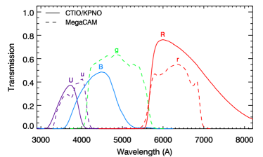
Figure 1: The transmission profiles for the filter combinations used at KPNO/CTIO (solid curves - $UBR$) and CFHT (dashed curves - $ugr$).

Conversions from the MegaCAM filter set to the SDSS filter set are given in the CFHT MegaCAM technical documentation, whilst conversions from the SDSS filter set to the Johnson-Cousins system are given by Fukugita et al. (1996). Combining these two sets of relations gives the following conversions between the two filter systems used in this work:

$$(u^{*}-g^{\prime})=1.05(U-B)+1.10$$ (1)

$$(g^{\prime}-r^{\prime})=0.57(B-R)-0.22$$ (2)

These relations are used throughout this paper where comparing the MegaCAM and Johnson-Cousins colours.

2.2.3 Photometry

Photometric zeropoints for the imaging fields were determined from standard star observations carried out as part of each of the imaging runs. The standard star fields were reduced in the same way as the science frames to ensure consistency. Source detection in the science images was performed with SExtractor (Bertin & Arnouts, 1996), using a 1.5$\sigma$ detection threshold and a 5-pixel minimum size.

Figure 2: Upper panel: Galaxy number counts in the $U$ (left), $B$ (middle) and $R$ (right) band imaging for the fields Q0301 (diamonds), Q2231 (triangles) and Q2359 (squares). Lower panel: Estimated completeness for each of the above bands based on simulated point sources (solid lines) and Vaucouleurs profile sources (dashed lines).

The $U_{Vega}$, $B_{Vega}$ and $R_{Vega}$ band galaxy number counts in the Q0301 (diamonds), Q2231 (triangles) and Q2359 (squares) LBG fields are shown in the top panels of Fig. 2. Stars were removed from these counts at magnitudes brighter than $\approx 22$ using a limit on the measured half-light radius of the sources. At fainter magnitudes, no attempt to remove stars from the counts was made, as the smallest extended sources become unresolved at the PSF of our fields at such magnitudes. We also show completeness estimates for each image in each field. These are estimated by placing simulated sources at random positions in a given image and measuring the fraction that are successfully extracted with SExtractor (using the same extraction parameters as used to create the full catalogues). In each case we estimate the completeness using both simulated point-sources and extended sources, where the extended sources are modelled by a de Vaucouleurs $r^{1/4}$ profile with a half-light radius of $r_{1/2}=0.3^{\prime\prime}$. In both cases, the simulated source is convolved with the image PSF before being added to the observation.

The results of the completeness estimates for the $UBR_{Vega}$ filter fields are shown in the lower panels of Fig. 2. The same symbols as the top panels are used for the different fields, whilst the dashed curves show the completeness estimates based on the extended sources and the solid curves show the completeness for the simulated point-sources. The 50% limits completion estimates (equivalent to $\approx 3\sigma$ detection limits) are given in Table 2. Comparing the completeness measurements across the fields, the measurements are relatively consistent with the imaging in each field reaching comparable depths. We note that given the compact nature of the LBG targets, the point source completeness levels should be a good representation of the true completeness. As such all our fields reach depths of $R>25$.

Figure 3: Number counts (top) and completeness estimates (bottom) in the $u$ (left), $g$ (middle) and $r$ (right) bands from the MegaCAM imaging on the HE0940-1050 and Q2348-011 fields.

We show the galaxy number counts (top panels) and completeness estimates (lower panels) for the MegaCAM fields in Fig. 3. Again the symbols are consistent between top and lower panels with the diamonds showing the results for the HE0940 field and the triangles showing the Q2348 field. As before, the solid lines in the lower panels show the completeness estimates for the point-like sources and the dashed lines show the same for the extended sources (which use the same de Vaucouleurs profile as used for the $UBR_{Vega}$ fields). Comparing the two fields to each other, the depths reached are comparable in each band, although the HE0940 is marginally less deep in the $u$ band by $\approx 0.5$ mag.

2.3 Candidate selection

2.3.1 $UBR$ selection

In the Q2359, Q0301 and Q2231 fields, we selected LBG candidates based on their $U$, $B$ and $R$ photometry. The criteria used were the same as those used by Paper I, which are based on those of Steidel et al. (2003). There are 4 groups to the selection, designated lbg_pri1, lbg_pri2, lbg_pri3 and lbg_drop and defined as follows:

lbg_pri1

• $23<R\leq 25$

• $0.5<(U-B)<4.0$

• $(B-R)<0.8(U-B)+0.6$

• $(B-R)<2.2$

lbg_pri2

• $23<R\leq 25$

• $(U-B)>0.0$

• $(B-R)<0.8(U-B)+0.8$

• $-1<(B-R)<2.7$

• $\notin$ lbg_pri1

lbg_pri3

• $23<R\leq 25$

• $-0.5<(U-B)<0.0$

• $-1.0<(B-R)<0.8(U-B)+0.6$

• $\notin$ {lbg_pri1,lbg_pri2}

lbg_drop

• $23<R\leq 25$

• $0.5<(B-R)<2.2$

• No detection in $U$

The first 3 groups represent an order of priority — that is, lbg_pri1 candidates are considered more likely to be $z\approx 3$ LBGs than e.g. lbg_pri3 candidates. This is because whereas lbg_pri1 tends to select outliers in the $UBR$ colour–colour plot, the lower priority groups select objects increasingly close to the colour region populated by stars and lower redshift galaxies, and therefore suffer from increased contamination from lower-redshift interlopers.

The fourth group is somewhat separate, being for galaxies which are not detected in the $U$ band. Such sources may be excellent LBG candidates, since it may be that the presence of the Lyman limit in the $U$ band has made the galaxy extremely faint in this band, such that it ‘drops out’ below the magnitude limit. However, the lbg_drop population is also likely to suffer from contamination, in this case because objects with no counterpart in 1 of the 3 bands have a higher chance of being spurious sources.

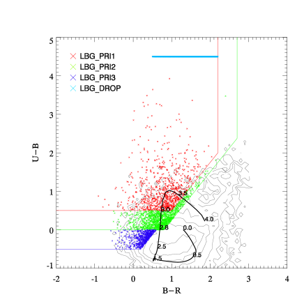
Figure 4: $UBR$ colour-colour plot showing candidate selection in Q2359. Objects selected as lbg_pri1, lbg_pri2, lbg_pri3 and lbg_drop candidates are shown in different colours as indicated by the legend. The lbg_drop candidates have been placed at $U-B=4.5$. The contours show the colour distribution of the rest of the objects in the field.

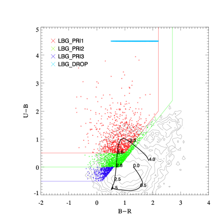
Figure 5: As for Fig. 4, but for Q0301.

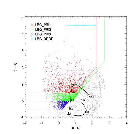
Figure 6: As for Fig. 4, but for Q2231.

Figs. 4, 5 and 6 show $UBR$ colour–colour plots for Q2359, Q0301 and Q2231, respectively. In each plot, the lbg_pri1, lbg_pri2, lbg_pri3 and lbg_drop candidates are indicated. A model colour–redshift track is also plotted, showing the expected evolutionary path of a star-forming galaxy from $z=0$ to $z=4$. This was produced using the Bruzual & Charlot (2003) model, assuming a Chabrier IMF and an exponential SFR with e-folding time $\tau=9$ Gyr. The model indicates that our selection criteria (across all the priority groups) is predicted to isolate galaxies in the range $\approx 2.5<z<3.8$. It also suggests that, of the sources that are confirmed as high-redshift LBGs, the lbg_pri3s should typically be at a lower redshift than the lbg_pri2s, which in turn should be at lower redshift than the lbg_pri1s. Paper I noted that this trend was detected in their LBG sample.

2.3.2 $ugr$ selection

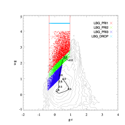
Figure 7: A $ugr$ colour-colour plot showing the selection of candidates in HE0940. Symbols are as in Fig. 4.

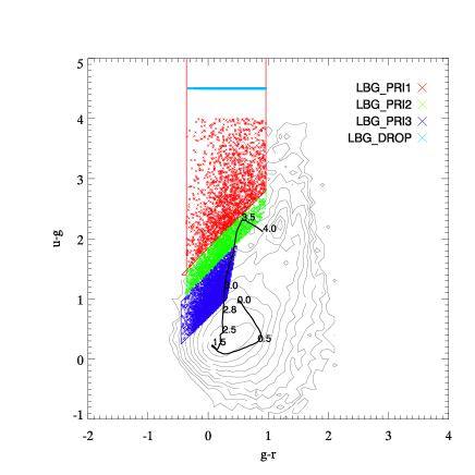
Figure 8: As for Fig. 7, but for Q2348.

In HE0940 and Q2348, LBG candidates were selected based on $ugr$ photometry. We have therefore adapted the criteria outlined above to account for the different colour bands. Again candidates were selected as either lbg_pri1, lbg_pri2, lbg_pri3 or lbg_drop, defined as follows:

lbg_pri1

• $23<r\leq 25$

• $1.4<(u-g)<4.0$

• $-0.36<(g-r)<0.96$

• $(g-r)<(u-g)-1.88$

lbg_pri2

• $23<r\leq 25$

• $(u-g)>1.0$

• $-0.36<(g-r)<0.96$

• $(g-r)<(u-g)-1.44$

• $\notin$ lbg_pri1

lbg_pri3

• $23<r\leq 25$

• $(g-r)<(u-g)-0.7$

• $-0.45<(g-r)<0.2(u-g)+0.1$

• $\notin$ {lbg_pri1,lbg_pri2}

lbg_drop

• $23<r\leq 25$

• $-0.36<(g-r)<0.96$

• No detection in $u$

Figs. 7 and 8 show the resulting candidates on $ugr$ colour-colour plots, and Table 3 gives the numbers and sky densities of candidates in all 5 LBG fields.

2.3.3 Comparing the LBG selections

The $UBR$ and $ugr$ selections have been developed to mimic the LBG selection of Steidel et al. (2003) and the BX selection of Adelberger et al. (2004). However, given the different sets of filters, the selection functions used here may not perfectly reproduce the original selections. For reference we show the selection functions used here overlayed on the original LBG and BX selections (transformed to the Vega $UBR$ system using the relations given by Steidel & Hamilton 1993) in Fig. 9. The CTIO/KPNO filter and CFHT MegaCAM filter (transformed to $UBR$ using the relations given on the CFHT website combined with those of Fukugita et al. 1996) selections are seen to agree well with the original Steidel et al. (2003) and Adelberger et al. (2004) selections. We note that we do not cover the entire of the Adelberger et al. (2004) BX region as doing so would bring a greater fraction of $z\lesssim 2$ galaxies. In addition, our $UBR$ selection boundaries extend somewhat further in the positive $B-R$ extent. This region is populated by few galaxies in the $23<R\leq 25$ range as evidenced by Figs. 4, 5 and 6, but is included to catch faint galaxies that have been scattered in colour space due to photometric errors.

In terms of the resulting space densities, the LBG_PRI1, LBG_PRI2 and LBG_DROP combined for the five fields give a mean space density of 2.00 arcmin^-2 for $R\leq 25$, marginally higher than the combination of the C, D, M and MD LBG selections of Steidel et al. 2003 that give a mean sky density of $\sim 1.8$ arcmin^-2 for ${\cal R}<25.5$. Taking the LBG_PRI3 candidates, we obtain a mean sky density of 0.37 arcmin^-2 in the $UBR$ fields and 1.38 arcmin^-2 in the $ugr$ fields. The LBG_PRI3 selection is intended to provide additional galaxies at $2<z<2.5$ and overlaps to some extent with the Adelberger et al. (2004) BX selection (as illustrated in Fig. 9). As expected the number densities here for the LBG_PRI3 selection are much lower than the BX selection, which obtains numbers of $\sim 5$ arcmin^-2 at ${\cal R}<25.5$, due to only sampling a subset of the BX selection.

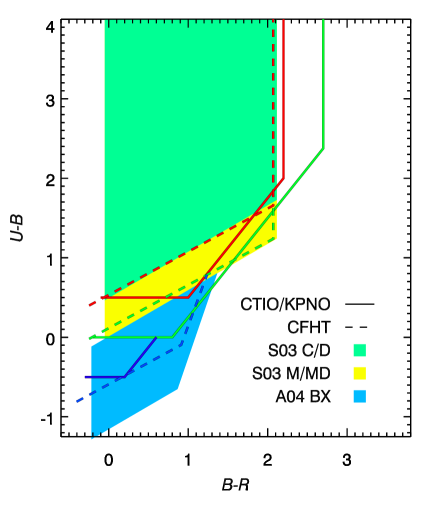
Figure 9: Comparison of the $UBR$ and $ugr$ selections compared to the original Steidel et al. (2003, green and yellow filled regions) LBG and Adelberger et al. (2004, cyan filled region) BX $U_{n}GR$ selections. All three are presented in the Vega $UBR$ system.

Table 3: Numbers and sky densities of $z\approx 3$ LBG candidates in each of the fields. For each priority class, the first column shows the total number of candidates selected and the second, italicised column shows the density in arcmin^-2. The last two columns show the figures for all $z\approx 3$ LBG candidates.

Field	lbg_pri1		lbg_pri2		lbg_pri3		lbg_drop		All
Q2359+0653	795	0.61	1,130	0.87	549	0.42	709	0.55	3,183	2.45
Q0301-0035	891	0.69	1,227	0.95	433	0.33	1,014	0.78	3,565	2.75
Q2231+0015	748	0.65	948	0.82	424	0.37	514	0.45	2,634	2.29
HE0940-1050	2,657	0.69	1,896	0.49	5,370	1.40	3,663	0.96	13,586	3.54
Q2348-011	1,843	0.52	1,624	0.46	4,808	1.35	1,850	0.52	10,125	2.84

2.4 Spectroscopy

2.4.1 Observations

The LBG candidates were targeted in spectroscopic follow-up observations with the VLT VIMOS spectrograph between September 2008 and December 2009, with programme IDs 081.A-0418(B) (Q2231), 081.A-0418(D) (Q2359), 081.A-0418(F) (Q0301), 082.A-0494(B) (HE0940) and 082.A-0494(D) (Q2348). The observations were done during dark time in generally good conditions with a typical seeing of $\approx 1$^′′ and an airmass of 1.0–1.3. Table 4 gives details of all the fields observed.

The VIMOS instrument (Le Fèvre et al., 2003) comprises four separate CCDs, each with a field of view of $7^{\prime}\times 8^{\prime}$. These four arms are arranged in a $2\times 2$ grid with a $\approx 2^{\prime\prime}$ gap between each CCD, giving a total $16^{\prime}\times 18^{\prime}$ FoV as quoted previously. Of this 288 arcmin² field, 224 arcmin² is covered by the detector.

Our observations utilised the low resolution blue (LR_Blue) grism and the order sorting blue (OS_Blue) filter, resulting in a wavelength range of 3700Å–6700Å, blazing at $\approx$4000Å. This wavelength range is ideal for our survey, detecting the Ly$\alpha$ line at $2.0<z<4.5$. The resolving power of the spectrograph in this configuration is $R=180$ assuming a 1^′′ slit (as used in these observations), which gives a resolution element of $\Delta\lambda\approx 22$Å at the blaze wavelength. The spectral dispersion is 5.3Å/pixel.

Table 4: Details of spectroscopic observations for the LBG target fields presented in this paper.

Field	Subfield	RAa	Deca	Exposureb	Airmass	Seeing	Dates
Q2359	f1	00:01:09.94	+07:03:26.8	10	$1.1-1.2$	$0.6-1.7$′′	23–25 Sep 2008
Q2359	f2	00:01:12.92	+07:16:39.2	10	$1.1-1.3$	$0.6-1.3$′′	3, 20–21 Oct 2008
Q2359	f3	00:02:11.50	+07:15:33.9	10	$1.2-1.4$	$0.6-1.3$′′	3, 21–25 Nov 2008
Q2359	f4	00:02:12.89	+07:02:19.1	10	$1.2-1.3$	$0.5-1.1$′′	26–30 Nov 2008
Q2231	f1	22:34:28.19	–00:06:03.3	10	$1.1-1.2$	$0.5-1.0$′′	23, 28 Oct 2008
Q2231	f2	22:34:28.55	+00:06:13.2	10	$1.1-1.2$	$0.4-0.9$′′	21–22 Oct 2008
Q2231	f3	22:33:39.51	–00:06:10.8	10	$1.1-1.2$	$0.5-1.0$′′	3 Aug; 27 Jul 2008
Q0301	f1	03:04:20.12	–00:14:28.8	12	$1.1-1.3$	$0.7-1.2$′′	23, 31 Oct 2008
Q0301	f2	03:03:10.27	–00:16:18.7	12	$1.1-1.2$	$0.7-1.5$′′	21–23 Nov 2008
Q0301	f3	03:03:15.41	–00:30:40.0	12	$1.1-1.2$	$0.7-1.5$′′	25–26 Nov 2008
Q0301	f4	03:04:15.56	–00:28:59.1	12	$1.1-1.2$	$0.7-1.2$′′	24 Sep; 1, 7 Oct 2008
HE0940	f4	09:42:10.00	–10:54:30.3	11.2	$1.0-1.3$	$0.8-1.5$′′	1 Feb 2009
HE0940	f5	09:43:07.47	–11:24:50.3	11.2	$1.0-1.3$	$0.7-1.4$′′	3 Feb 2009
HE0940	f6	09:41:59.99	–11:24:50.4	11.2	$1.0-1.2$	$0.5-1.2$′′	20–21 Feb 2009
HE0940	f7	09:44:14.99	–11:24:49.9	11.2	$1.0-1.2$	$0.5-1.3$′′	22, 24 Feb 2009
HE0940	f8	09:43:21.49	–10:41:00.5	11.2	$1.0-1.2$	$0.5-1.0$′′	26–27 Feb 2009
HE0940	f9	09:42:09.99	–10:40:59.8	11.2	$1.0-1.3$	$0.5-1.2$′′	2 Feb 2009
Q2348	f1	23:51:50.08	–00:54:21.9	11.5	$1.1-1.2$	$0.5-1.7$′′	23–25 Jul 2009
Q2348	f2	23:50:45.09	–00:54:22.2	11.5	$1.0-1.1$	$0.5-1.0$′′	19–20 Jul 2009
Q2348	f3	23:49:40.07	–00:54:22.6	11.5	$1.0-1.2$	$0.4-0.8$′′	27 Jul 2009
Q2348	f4	23:51:50.12	–00:37:31.6	11.5	$1.1-1.2$	$0.5-1.5$′′	20–21 Aug 2009
Q2348	f5	23:50:45.05	–00:37:31.5	11.5	$1.0-1.2$	$0.7-1.4$′′	16–20 Sep 2009
Q2348	f6	23:49:40.00	–00:37:32.0	11.5	$1.1-1.2$	$0.8-1.3$′′	24–25 Sep 2009
Q2348	f7	23:51:50.12	–01:07:31.4	11.5	$1.1-1.2$	$0.7-1.0$′′	12, 20 Oct 2009
Q2348	f8	23:50:45.00	–01:07:32.0	11.5	$1.1-1.3$	$0.7-1.3$′′	22 Nov, 10 Dec 2009
Q2348	f9	23:49:40.00	–01:07:32.0	11.5	$1.1-1.3$	$0.8-1.5$′′	15–22 Nov 2009
a J2000 coordinates of subfield centre
b in ks

The slit masks were designed using the vmmps software which is standard for VIMOS observations. The aims for mask design are (a) to maximise the number of observed targets, (b) to favour higher-priority targets and (c) to ensure slits are of sufficient size to allow a robust sky subtraction. Since these aims are frequently in conflict with one another, the mask design process is one of attempting to optimise the observations to satisfy all three as well as possible. Point (c) is addressed by setting a minimum slit length of 8^′′ (40 pixels given the pixel scale of 0.205^′′/pixel). Slit length was increased as much as possible where such an increase would not prevent the observation of an additional target — that is, where it did not conflict with point (a). Finally, in order to optimise slit allocation, some targets were added to fill gaps that fulfilled the given selection criteria, but with fainter $R$ magnitudes down to a limit of $R=25.5$.

With the LR_Blue grism, each spectrum spans 640 pixels along the dispersion axis. Assuming a 40 pixel slit width as specified above, this would allow for a possible total of over 300 slits on the full 4k$\times$2k detector. This is however not practically achievable given the density of LBG candidates, and is hampered further by the need to select high-priority candidates (point b), which have an even lower sky density. Our final slit masks therefore typically contain some 50–70 slits per quadrant.

2.4.2 Data reduction

The spectroscopic data have all been reduced using the VIMOS esorex reduction pipeline. Using bias frames, flat fields and arc lamp exposures taken for each mask during each observing run, the pipeline generates bias-subtracted, flat-fielded, wavelength-calibrated science frames consisting of a series of 2D spectra. Following Paper I we use the imcombine procedure in iraf to combine the reduced frames from each observing block, generating a master science frame for each quadrant of each field. When combining the frames we use the crreject mode, designed to remove cosmic rays by rejecting pixels with significant positive spikes. We have also used the avsigclip rejection mode with a rejection threshold of $3\sigma$, and find that our results are not significantly affected, suggesting that our results do not depend strongly on the parameters used to combine the science frames at this stage.

We extract 1D spectra from the reduced, combined 2D spectra using the idl routine specplot. One-dimensional object and sky spectra are found by averaging across the respective apertures, and the sky spectrum is then subtracted from the object spectrum to give a final spectrum for the object.

In some cases there remain significant sources of contamination in the final object spectrum. These can arise from bad pixels, either in the object or sky aperture, from contamination from the zeroth order from other slits, or more frequently from the bright sky emission lines [O i] 5577Å, [Na i] 5990Å and [O i] 6300Å; in either case, the resulting contamination may manifest itself as either a positive or a negative spike in the spectrum. Such artefacts are, however, easily spotted during a routine inspection of the 2D spectrum.

2.5 Identification of targets

Every source targeted for spectroscopic observation is inspected visually, in both the 2D and 1D spectra, to determine where possible a redshift and classification. Sources are classified as either $z\approx 3$ Lyman-break galaxies, low-redshift galaxies, QSOs or Galactic stars. The LBGs are divided into those showing Ly$\alpha$ emission (designated LBe) and those showing Ly$\alpha$ absorption (LBa). QSOs are determined by the presence of typical AGN emission features, in particular Ly$\alpha$ and C IV. Stars are classified by comparison to template spectra: in particular we check for A, F, G, K and M stars.

In determining the redshift and classification the spectral feature primarily used in the case of LBGs is the Ly$\alpha$ emission/absorption line at 1216Å; for lower redshift galaxies it is the [O ii] emission line at 3727Å. In addition to these, some of the following features are used:

For $z\approx 3$ LBGs:

• Lyman limit, 912Å;

• Ly$\beta$ emission/absorption, 1026Å

• O VI 1032Å, 1038Å;

• Ly$\alpha$ forest, $<$1215.67Å;

• Ly$\alpha$ emission/absorption, 1215.67Å;

• Inter-stellar medium (ISM) absorption lines:

  • Si II 1260.4Å;

  • O I$+$Si II 1303Å;

  • C II 1334Å;

  • Si IV doublet 1393Å & 1403Å;

  • Si II 1527Å;

  • C IV doublet absorption, 1548-1550Å.

  • Fe II 1608Å;

  • Al II 1670Å;

For low-$z$ galaxies:

• CN absorption 3833Å;

• K-band absorption 3934Å;

• HK break 4000Å;

• H$\delta$ emission 4102Å;

• H$\beta$ emission/absorption 4861Å;

• O iii emission 4959Å;

• O iii emission 5007Å;

The presence of the HK break causes these interlopers to appear fairly frequently in our spectroscopic samples, since these features mimic the Lyman break on which our selection is based. The ISM absorption features listed above for LBGs are therefore of considerable importance in identifying genuine $z\approx 3$ galaxies. For every target which is identified, we assign a quality parameter to the redshift determined, in the range $0\leq Q\leq 1$. A quality of $Q\leq 0.4$ indicates that a possible redshift has been determined, but is not considered a robust measurement. Above this, for LBGs, the quality parameters indicate that the redshift is based on the following features:

• $Q=0.5$ — a spectral break with some weak Ly$\alpha$ emission/absorption and low-SNR ISM absorption features, or strong Ly$\alpha$ emission but with no detected continuum

• $Q=0.6$ — a spectral break with high-SNR Ly$\alpha$ emission/absorption plus low-SNR ISM absorption features

• $Q=0.7$ — a spectral break with high-SNR Ly$\alpha$ emission/absorption plus unambiguous, high-SNR ISM absorption features

• $Q=0.8$ — a spectral break with high-SNR Ly$\alpha$ emission/absorption plus high-SNR absorption and lower-SNR emission lines (e.g. Si ii 1265Å, 1309Å; He ii 1640Å)

• $Q=0.9$ — as for Q=0.8, but reserved for highest signal-to-noise objects only

Table 5: Example LBG identifications in the Q2359+0653.

ID	R.A.	Dec.	$U-B$	$B-R$	$R$	$z_{Ly\alpha}$	$z_{ISM}$	$Q_{ID}$
	(J2000)
VLRS J000139.85+070221.66	0.4160563	7.0393505	0.63	0.76	23.5500	2.4762	2.4682	0.5
VLRS J000133.54+070127.57	0.3897395	7.0243263	0.13	0.15	25.3600	2.5707	2.5603	0.5
VLRS J000118.84+070106.55	0.3285175	7.0184855	1.29	1.21	23.8900	3.0374	3.0294	0.5
VLRS J000131.05+070106.56	0.3793770	7.0184898	0.58	0.65	25.3900	2.7910	2.7967	0.5
VLRS J000141.27+070106.35	0.4219468	7.0184293	1.51	0.12	24.3800	2.6508	2.6428	1.0
VLRS J000140.69+070044.11	0.4195270	7.0122533	0.47	0.65	23.7800	2.8162	2.8082	0.5
…	…	…	…	…	…	…	…	…
…	…	…	…	…	…	…	…	…

Table 6: Example LBG identifications in the Q0301-0035.

ID	R.A.	Dec.	$U-B$	$B-R$	$R$	$z_{Ly\alpha}$	$z_{ISM}$	$Q_{ID}$
	(J2000)
VLRS J030434.85-001549.27	46.1452103	-0.2636854	0.59	0.61	24.4700	2.6132	2.6041	0.7
VLRS J030435.40-001607.15	46.1474953	-0.2686527	1.56	1.45	23.4100	2.5969	2.6157	0.7
VLRS J030439.49-001619.35	46.1645317	-0.2720422	1.08	0.62	24.5100	2.9570	2.9490	0.5
VLRS J030438.22-001647.63	46.1592560	-0.2798966	-0.22	0.37	23.8600	2.7098	2.7292	0.6
VLRS J030435.86-001654.14	46.1494179	-0.2817046	0.80	0.92	25.0700	2.8887	2.8807	1.0
VLRS J030426.38-001701.38	46.1099281	-0.2837157	0.21	0.56	24.4900	2.4651	2.4571	0.6
…	…	…	…	…	…	…	…	…
…	…	…	…	…	…	…	…	…

Table 7: Example LBG identifications in the HE0940-1050.

ID	R.A.	Dec.	$u-g$	$g-r$	$r$	$z_{Ly\alpha}$	$z_{ISM}$	$Q_{ID}$
	(J2000)
VLRS J094225.83-105744.50	145.6076355	-10.9623623	2.57	0.35	23.6400	2.8804	2.8810	0.5
VLRS J094240.69-105753.44	145.6695251	-10.9648447	1.88	0.35	24.1100	3.1456	3.1376	0.5
VLRS J094220.01-105900.05	145.5833588	-10.9833469	—	-0.14	24.3800	2.2010	2.1930	0.5
VLRS J094217.39-105923.95	145.5724640	-10.9899855	—	0.16	23.8500	2.5153	2.5073	0.5
VLRS J094217.51-105935.92	145.5729675	-10.9933100	—	0.79	24.2600	2.8139	2.8119	0.6
VLRS J094242.29-110121.16	145.6762085	-11.0225439	0.74	-0.03	23.9900	2.4613	2.4595	0.5
…	…	…	…	…	…	…	…	…
…	…	…	…	…	…	…	…	…

Table 8: Example LBG identifications in the Q2231+0015.

ID	R.A.	Dec.	$U-B$	$B-R$	$R$	$z_{Ly\alpha}$	$z_{ISM}$	$Q_{ID}$
	(J2000)
VLRS J223439.00+000341.29	338.6625061	0.0614693	—	0.72	24.1500	2.8428	2.8291	0.6
VLRS J223459.87+000308.07	338.7494507	0.0522424	1.01	0.78	23.7400	2.4879	2.4789	0.5
VLRS J223450.20+000232.38	338.7091675	0.0423284	—	1.92	23.7800	2.8934	2.8927	0.7
VLRS J223459.03+000051.79	338.7459717	0.0143855	—	0.54	24.3200	2.8037	2.7957	0.9
VLRS J223442.76-000028.59	338.6781616	-0.0079414	0.32	1.01	23.6900	2.1897	2.1817	0.5
VLRS J223447.81-000041.63	338.6991882	-0.0115636	—	0.87	24.8000	2.8874	2.8735	0.5
…	…	…	…	…	…	…	…	…
…	…	…	…	…	…	…	…	…

Table 9: Example LBG identifications in the Q2348-011.

ID	R.A.	Dec.	$u-g$	$g-r$	$r$	$z_{Ly\alpha}$	$z_{ISM}$	$Q_{ID}$
	(J2000)
VLRS J235206.92-005646.70	358.0288391	-0.9463067	1.30	0.30	24.4600	3.1430	2.3707	0.5
VLRS J235200.98-005903.11	358.0040894	-0.9841969	2.50	0.46	24.2400	3.3532	3.3435	0.5
VLRS J235201.68-010002.18	358.0069885	-1.0006067	1.23	0.31	24.9700	2.8632	2.8603	0.5
VLRS J235155.14-010104.04	357.9797363	-1.0177902	1.66	0.15	23.8600	2.7523	2.7503	0.7
VLRS J235209.28-005535.49	358.0386658	-0.9265237	1.28	0.13	24.0700	2.6274	2.6194	0.7
VLRS J235202.62-004747.89	358.0109253	-0.7966368	2.11	0.32	24.2700	3.0640	3.0646	0.5
…	…	…	…	…	…	…	…	…
…	…	…	…	…	…	…	…	…

2.6 LBG sample

2.6.1 Sky densities, redshift distributions and completeness

In total, the VLRS now consists of 2,135 spectroscopically confirmed LBGs in $\approx$ 10,000 arcmin² (a density of $\approx$ 0.20 arcmin^-2). 1,994 of these are within a magnitude limit of $R\leq 25$, whilst the remainder form a non-uniform sample of $25<R\leq 25.5$ LBGs that were observed as part of optimising slit allocations in the spectroscopic observations. We show the sky distribution of LBGs from both Paper I (open grey circles) and this paper (filled black circles) for all nine VLRS fields in Fig. 10. Known QSOs in the fields are also plotted (cyan stars). The total numbers of $R\leq 25$ $Q\geq 0.5$ sources identified in each of the 5 fields presented here are given in Table 10. We present examples of the first six LBGs in each of the fields in Tables 5 to 9. The full tables will be made available online at http://star-www.dur.ac.uk/$\sim$bielby/vlrs/.

For the $z>2$ sample, the VLRS now consists of 944 $Q=0.5$, 492 $Q=0.6$, 318 $Q=0.7$, 147 $Q=0.8$ and 93 $Q=0.9$ galaxies at a magnitude limit of $R\leq 25$.

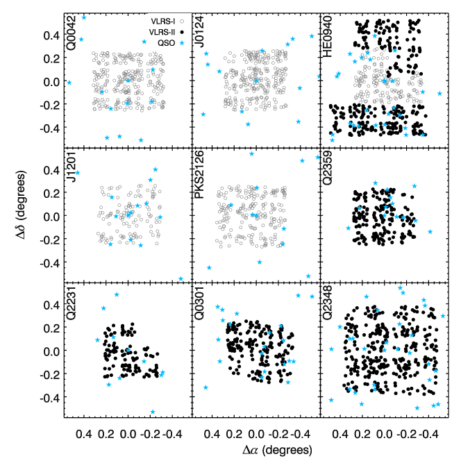
Figure 10: Sky distribution of LBGs and QSOs in the VLRS fields. Grey open circles show LBGs presented in Paper I, black filled circles show LBGs identified in the current work and cyan stars show known QSOs.

Table 10: Numbers of objects in each target field spectroscopically identified at $Q\geq 0.5$ and $R\leq 25$ as either high-$z$ LBGs, $z<2$ galaxies, AGN/QSOs, stars or unidentified.

Field	$z\approx 3$ LBGs	$z<2$ galaxies	QSO/AGN	Stars
Q2359	143 (0.18 arcmin-2)	67	5	8
Q0301	164 (0.21 arcmin-2)	61	10	13
Q2231	108 (0.18 arcmin-2)	80	6	18
HE0940	358 (0.30 arcmin-2)	186	4	48
Q2348	303 (0.17 arcmin-2)	100	11	34
Total	1,076 (0.21 arcmin-2)	494	36	121

Fig. 11 shows the $n(z)$ distributions of all sources with measured redshifts in each of the 5 LBG fields. The figure shows that LBGs in HE0940 and Q2348, where LBGs were selected in $ugr$, have higher average redshifts than in the $UBR$-selected fields, suggesting that the $ugr$ criteria bias the selection toward higher $z$. It is also notable from Table 10 that the $ugr$ selection appears to include more Galactic stars. Future $ugr$-selected LBG surveys may wish to alter our colour criteria to better avoid stellar interlopers.

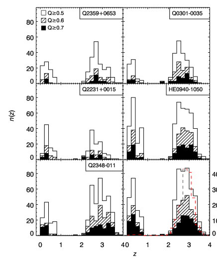
Figure 11: Redshift distributions of identified sources in each of the target fields (first five panels) and for the whole sample of 1,994 $R\leq 25$ galaxies (bottom right panel). In each panel we show the distribution for the full sample ($Q\geq 0.5$), as well as for the $Q\geq 0.6$ (hashed) and $Q\geq 0.7$ (filled) subsets, where $Q$ is the redshift quality parameter. In the final panel, we also show the redshift distribution of the Steidel et al. (2003) galaxies used in this work (dashed red line).

Fig. 11 also shows $n(z)$ for the subsets of sources with $Q\geq 0.6$ and $Q\geq 0.7$. We note that in any given field, the distributions of sources at $Q\geq 0.5$, $Q\geq 0.6$ or $Q\geq 0.7$ are approximately the same — the LBGs with higher ID qualities are not skewed to lower or higher redshift, for example — suggesting that the redshift distributions shown are fairly robust. The average redshifts and standard deviations are given in Tab. 11. The redshift distribution of the full LBG sample has a mean redshift of $2.79\pm 0.01$ and a standard deviation of 0.34, and is shown in the lower right panel of Fig. 11.

Table 11: Redshift distribution statistics for spectroscopically confirmed, $R\leq 25$ $Q\geq 0.5$ LBGs in the 5 observed fields. In each case the mean redshift $\bar{z}$ (with standard error), median redshift $\tilde{z}$ and standard deviation $\sigma$ of the distribution is given.

Field	$\bar{z}$	$\tilde{z}$	$\sigma$
Q2359	$2.81\pm 0.03$	$2.74$	$0.36$
Q0301	$2.64\pm 0.02$	$2.59$	$0.31$
Q2231	$2.68\pm 0.03$	$2.65$	$0.30$
HE0940	$2.79\pm 0.02$	$2.77$	$0.34$
Q2348	$2.90\pm 0.02$	$2.92$	$0.36$
Total	$2.79\pm 0.01$	$2.76$	$0.35$

Fig. 12 shows, as anticipated in §2.3, that candidates selected as lbg_pri1 lie at higher redshift than the lbg_pri2 candidates, which are in turn at higher redshift than lbg_pri3s. Quantitatively, we find that the lbg_pri1s have a mean redshift of $\bar{z}=2.83\pm 0.02$, the lbg_pri2s have $\bar{z}=2.71\pm 0.02$ and the lbg_pri3s have $\bar{z}=2.61\pm 0.02$. The lbg_drop candidates are shown in a separate panel for clarity, and have the highest mean redshift of all the groups, with $\bar{z}=2.93\pm 0.02$.

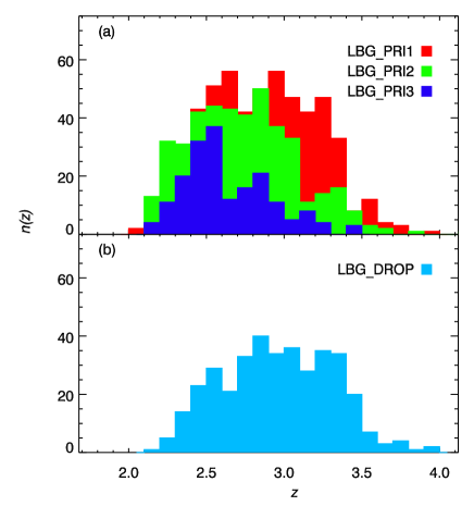
Figure 12: Redshift distribution of all identified sources our 5 target fields, separated by initial candidate priority. Panel (a) shows the lbg_pri1, lbg_pri2 and lbg_pri3 classes, while the lbg_drops are shown separately in panel (b) for clarity. Colours are as in Figs. 4–7.

In total, for the $R\leq 25$ targets, we make successful identifications in $\approx 30\%$ of VIMOS slits and of those identified, $62\%$ are identified as $z>2$ galaxies. In terms of the unidentified fraction, these are likely predominantly faint $z>2$ galaxies (most likely dominated by dusty, absorbed galaxies with no Ly$\alpha$ emission) and relatively featureless $1\lesssim z\lesssim 2$ galaxies. We note that the $38\%$ contamination rate is somewhat higher than that quoted for the Steidel et al. (2003) and subsequent samples. This is in part likely the result of the shallower depths and differing filters used in the colour selections. Additionally, following the results of other authors (e.g. Reddy et al., 2008), it is likely that the faint population that has avoided identification in our observations is less prone to contamination and as such likely has a higher percentage of $z\sim 3$ galaxies than the $62\%$ measured for the sample in which we could successfully identify spectral features.

Breaking the contamination level into the different selections, we find that the LBG_PRI1, LBG_PRI2, LBG_PRI3 and LBG_DROP samples have contamination rates of 32.5%, 35.6%, 38.2% and 40.3% respectively. Based on these recovered levels of contamination (and making the simplifying assumption that this applies to the faint unidentified spectroscopic sample), gives an average sky-density across our fields of $\approx 1.8$ arcmin^-2 for all samples and $\approx 1.3$ arcmin^-2 excluding the LBG_PRI3 sample. Based on the volumes probed and the redshift distribution, these sky densities correspond to sky densities of $\sim 4.0~{}h^{3}$Mpc^-3.

2.7 Galaxy redshifts

In star-forming galaxies such as those presented here, the observed Ly$\alpha$ emission is redshifted relative to the intrinsic galaxy redshift, while the interstellar absorption lines are blue-shifted (see e.g. Shapley et al., 2003). In Paper I, we used the transformations given by Adelberger et al. (2005a) in order to correct from the redshifts of the UV features to the intrinsic galaxy redshifts. These have now been superseded by those determined in Steidel et al. (2010), which we use in this paper and also apply to our previous data from Paper I.

In Paper I, we estimated the errors on the LBG redshifts using simulated spectra. Here, we extend the investigation into the redshift errors in our survey by using duplicate redshift measurements. The fields presented here, particularly Q2348, were designed with overlapping regions and consequently there are some LBG candidates which were observed in more than one mask. In cases where these duplicated targets are confirmed as LBGs, this provides two independent redshift measurements for the same LBG, and thus a direct observational test of the redshift measurement accuracy.

Fig. 13 shows the $\Delta z$ distribution for the LBGs with duplicate observations, where $\Delta z=|z_{1}-z_{2}|$ is the difference between the two redshift measurements. A total of 20 objects were classified as LBGs in two separate observations; of these, Fig. 13 indicates that 16 had fairly small errors of $\Delta z<0.02$ (of which 13 had very small errors of $\Delta z<0.005$), while 4 had considerably larger errors. In addition to these 20 objects, we have also searched a region of our Q0301 field which overlaps with Steidel et al. (2003) survey for any LBGs which were identified in both surveys: we find 3 such objects, and the redshift differences for these galaxies are also indicated in Fig. 13.

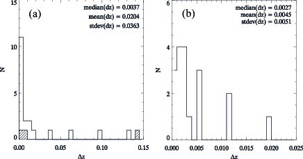
Figure 13: The distribution of redshift measurement errors, $\Delta z$, calculated using the LBGs which were observed twice in our survey and therefore have two independent redshift measurements. In panel (a) we show the full distribution, in panel (b) a close-up of the distribution at $z<0.025$. Overplotted as a hashed histogram in panel (a) are the $\Delta z$ values for 3 sources in our survey which had a redshift in the survey of Steidel et al. (2003).

The standard deviation of the 20 $\Delta z$ values measured for duplicate observations in our survey is $\sigma=0.036$, corresponding to a velocity error of $\approx$2,800 km s^-1 assuming a redshift of $z=2.8$, the sample mean. However, this misrepresents the true error in our redshift measurements, since it is skewed by the 4 sources with very high $\Delta z$. These 4 values do not represent redshift measurement errors, rather catastrophic outliers. In the cases where we find large $\Delta z$ values, the error does not arise due to uncertainty in the peak wavelength, but in uncertainty over which spectral feature is actually Ly$\alpha$. In these cases, different spectral features have been identified as Ly$\alpha$, leading to large $\Delta z$. These are therefore better characterised as identification errors, in that two different solutions have been reached in the two observations.

For the 16 duplicated targets shown in Fig. 13b, the same feature has been identified as Ly$\alpha$ and therefore the $\Delta z$ for these objects gives an indication of the measurement error. The standard deviation for these objects is $\sigma=0.005$, corresponding to $\Delta v\approx 380$ km s^-1.

The suggestion, therefore, is that $\approx$80% of our LBGs have redshift measurement errors of $\Delta v\leq 400$ km s^-1, while the other 20% may have larger errors. This problem, however, disproportionately affects sources with an ID quality parameter $Q=0.5$: of the four sources with large $\Delta z$, one was given a quality factor of 0.5 for both redshift measurements, while the other 3 have one measurement with $Q=0.5$ and another with $Q=0.6$; in the latter cases the $Q=0.6$ measurement is fairly robust while the $Q=0.5$ measurement is less reliable. Therefore, the LBGs which may suffer from large errors can be excluded by removing the $Q=0.5$ LBGs from the sample.

2.7.1 Composite spectra

We have calculated composite spectra using the $z>2$ VIMOS low-resolution galaxy data. The composite spectra were generated by averaging over the spectra after having corrected the spectra for the instrument response and having masked skylines. In addition, each individual spectrum is normalised by its median flux in the rest-frame wavelength range $1250\AA\leq\lambda\leq 1450$ before being combined to form the composite.

In Fig. 14 we show stacked spectra for the LBGs, separated into those showing Ly$\alpha$ in emission (lower panel) and in absorption (upper panel). These stacked spectra show the average ultraviolet SED of a $z\approx 3$ LBG with excellent signal-to-noise, and the quality of these spectra provide an indication of the robustness of our LBG identifications.

In Fig. 15, we show 3 separate composite spectra for sources classed as LBe’s with quality IDs of $Q=0.5$, $Q=0.6$ and $Q\geq 0.7$. These spectra reflect the quality criteria set out in §2.5 well, with increasing quality spectra clearly showing increasingly high signal-to-noise in both Ly$\alpha$ emission and ISM absorption features. In addition, the strength of the absorption features in the spectra appears to be systematically weaker with lower $Q$. This is likely the result of the lower signal-to-noise of the lower $Q$ identifications.

Finally we note that some potential flux is observed at wavelengths below the Lyman-limit, however even after stacking, the signal is subject to significant noise. Further analysis on the escape fraction may be possible using this data, but is beyond the scope of this paper.

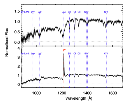
Figure 14: Composite spectra for galaxies showing Ly$\alpha$ in absorption (top) and emission (bottom), with ISM absorption lines clearly detected.

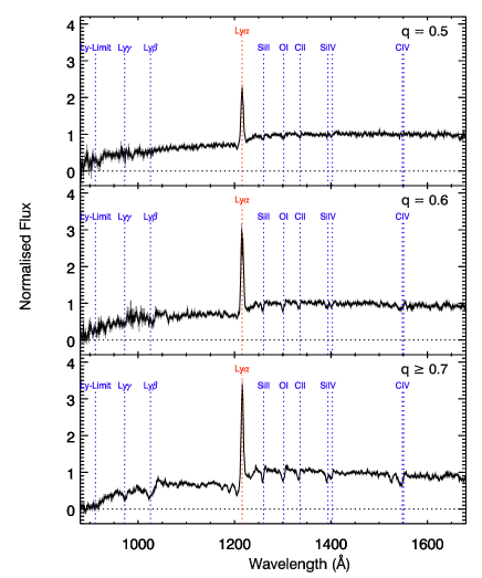
Figure 15: Composite spectra for galaxies classified as LBe’s, separated by ID quality parameter $Q$. Those with $Q=0.5$ (upper panel) show comparatively weak Ly$\alpha$ emission and marginal detections of ISM absorption lines. Moving to higher quality values, the strength of the Ly$\alpha$ line increases and we also see high-SNR absorption features. Note that the spectra are not flux calibrated.

2.7.2 Quasars & AGN

We have identified 33 $z>1.5$ AGN and QSOs in our spectroscopic sample, which we present here as part of the VLRS catalogue. They have been identified by the presence of strong Ly$\alpha$, C iv and C iii$+$Si iii emission lines as well as the generally weaker lines of O vi, N v and Si iv. Their spectra are shown in Fig. 16. The above emission lines are indicated in each panel of Fig. 16.

Several other emission lines are detected in some of the QSO spectra but are not marked in the figure. Ly$\beta$ $\lambda$1026 is clearly seen in panel (e), where it may be asymmetrically broadened to longer wavelengths by the presence of relatively weak O vi $\lambda$1035. Panel (p) shows an emission line peaking at 1029Å, likely suggesting a blend between Ly$\beta$ and O vi.

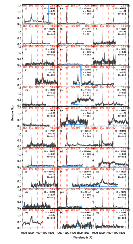
Figure 16: Rest-frame VIMOS spectra for the QSOs detected in the 5 fields presented. The $y$-axis scales differ from panel to panel, but the dotted line marks zero flux in each case. Dashed red lines indicate the wavelength of O vi, Ly$\alpha$, Ne v and C iv emission. Gaps in the spectra indicate that an artefact has been masked out.

Emission arising from the combination of O i $\lambda$1302 and Si ii 1304 is visible in a number of the spectra, for example in panels (a) and (h). Finally, many of the panels show clear emission at $\approx 1400$Å, arising from a blend of the Si iv $\lambda$1396 and O vi] $\lambda$1402 transitions.

The spectra show a clear mix of both broad and narrow line AGN, the narrow line objects suggestive of the presence of obscured AGN activity. These are reminiscent of the AGN identified in similar $z\sim 3$ star-forming galaxy surveys, for example Steidel et al. (2002); Hainline et al. (2011, 2012).

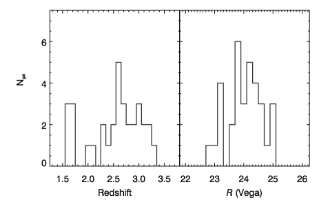
Figure 17: The redshift (left) and $R_{Vega}$ magnitude (right) distributions of the 33 serendipitous spectroscopically identified quasar/AGN sample.

The redshift distribution of the 33 $z>1.5$ AGN is shown in the left hand panel Fig. 17, whilst the $R$-band Vega magnitude distribution is shown in the right hand panel.

3 Clustering of $z\approx 3$ LBGs

We now analyse the clustering of the $z\approx 3$ LBGs. As well as offering insights into the growth and evolution of structure in the Universe, we aim to measure the dynamics of the $z\approx 3$ galaxy population, i.e. peculiar velocities and gravitational infall, to inform the analysis of the gas-galaxy relationship via LBG-Ly-$\alpha$ forest cross-correlation (see Paper II).

We note that for the purposes of the clustering analysis we use the 1,994 $R\leq 25$ VLRS sample (and place a limit of $R\leq 25.2$ on the Keck sample with which it is compared and combined). Aside from this magnitude cut, all galaxies with $Q\geq 0.5$ are included throughout this analysis. Taking the ${\cal R}=25.2$ limit for the Keck sample provides 815 galaxy redshifts within the Steidel et al. (2003) fields to combine with our VLRS sample.

In the analysis that follows, we measure the galaxy clustering as a function of galaxy-galaxy separation using the Landy-Szalay estimator:

$$\xi(x)=\frac{\left<\mathrm{DD}(x)\right>-2\left<\mathrm{DR}(x)\right>+\left<\mathrm{RR}(x)\right>}{\left<\mathrm{RR}(x)\right>}$$ (3)

where $\xi(x)$ is the clustering as a function of separation $x$, $\mathrm{DD}(x)$ is the number of galaxy-galaxy pairs at that separation, $\mathrm{DR}(x)$ is the number of galaxy-random pairs and $\mathrm{RR}(x)$ is the number of random-random pairs. This is estimated using a random catalogue that consists of 20$\times$ as many random points as data points and that covers an identical area. The redshift distribution of the random catalogue is set using a polynomial fit to the data.

We focus on fitting the auto-correlation function in the semi-projected, $w_{p}(\sigma)$, and full 2-D, $\xi(\sigma,\pi)$, forms, where $\sigma$ and $\pi$ are the separation of two galaxies transverse and parallel to the line-of-sight. But we shall also study the LBG $z$-space correlation function, $\xi(s)$, where the signal can be significantly higher at large scales.

For $\xi(\sigma,\pi)$ in particular, we also consider the combined sample of the VLRS data with the Keck LBG data of Steidel et al. (2003). The Keck data offers higher sampling rates than the VLRS, but across smaller field sizes ($\approx 8$^′). This is illustrated in Fig. 18 where the solid black line shows the VLRS pair counts (DD) as a function of separation in the transverse direction, $\sigma$ (left hand panel), and the 3-D separation, $s=\sqrt{\sigma^{2}+\pi^{2}}$ (right hand panel). In both panels the Keck pair counts are shown by the dashed orange line. Fig 18 shows that the VLRS pair counts in both the transverse and 3-D distance are significantly higher than in the previous Keck sample at $\sigma,s\ga 10$h^-1Mpc.

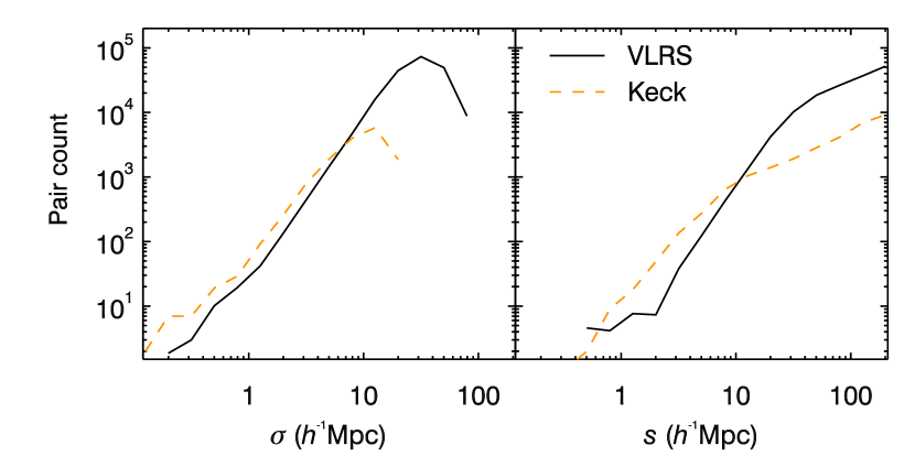
Figure 18: Pair counts (DDs) as a function of pair separation in the transverse, $\sigma$, and 3D Hubble, $s$, directions. The Keck data (dashed orange curves) provide better sampling at small scales, whilst the VLRS data (solid black curves) provides sampling at larger scales that is not provided by previous data.

On the validity of combining our own LBG sample with that of Steidel et al. (2003), we note that Steidel et al. (2003) used photometry with mean 1$\sigma$ depths of $\left<\sigma(U_{n})\right>=28.3$, $\left<\sigma(G)\right>=28.6$ and $\left<\sigma({\cal R})\right>=28.0$, whilst their imposed ${\cal R}$ band limit was ${\cal R}=25.5$. Using the transformations of Steidel & Hamilton (1993), the Steidel et al. (2003) 1$\sigma$ limits correspond to $U=27.55$, $B=28.77$ and $R=27.86$ in the Vega system. Comparing this to the average depths ascross all the VLRS fields, we have mean $3\sigma$ depths of $U=25.8$, $B=26.4$ and $R=25.9$, which equate to $1\sigma$ depths of $U=27.0$, $B=27.6$ and $R=27.1$, approximately 1 mag fainter in each band than the Steidel et al. (2003) imaging data. However, given our limit of $R=25$ (and our imposed ${\cal R}=25.2$ for the Keck sample), the $B-R$ (and $G-{\cal R}$) constraints on the selections, and the inclusion of galaxies with no $U$-detection, the VLRS and Keck samples will be relatively equivalent in terms of the galaxies included.

It is clear however, that the VLRS sample, although giving a close approximation of the Keck sample selections, is not a perfect replica of the Keck selection. Given the difference in the filters and the moderate difference in depths this was unlikely to ever be the case. The redshift distributions are relatively well matched, but (partially due to the addition of the LBG_PRI3 selection) the VLRS sample is skewed somewhat to marginally lower redshifts (as illustrated in Fig. LABEL:). Additionally, the sky and space densities are close but not perfectly matched, as are the $R-band$ magnitude distributions (as shown by Paper I, ). As a result, the UV luminosity functions will be similarly close but not perfectly matched. In combining the two samples we therefore note these differences and use the results of combining the samples with caution. However, it is beneficial to do so in order to help constrain the redshift-space distortion effects, which are an important element of further work incorporating the Ly$\alpha$ forest to constrain the distribution of gas around these star-forming galaxies. Furthermore, it is difficult to perform these tests with either sample alone given the Keck sample’s small area coverage and the VLRS sample’s comparatively lower sampling rate. Therefore, although the combination is not ideal, it offers an indication of the impact of redshift space distortions on the correlation functions that may be utilised in subsequent work.

3.1 Semi-projected correlation function, $w_{p}(\sigma)$

We first estimate the LBG clustering using the semi-projected correlation function, $w_{p}(\sigma)$. This gives the clustering at fixed transverse separation, $\sigma$, integrated over line-of-sight distance, $\pi$, approximately independent of the effect of peculiar velocities and is given by:

$$w_{p}(\sigma)=2\int^{\infty}_{0}\xi(\sigma,\pi)d\pi$$ (4)

where $\xi(\sigma,\pi)$ is the 2-D auto-correlation function. We integrate $\xi(\sigma,\pi)$ over the range $0<\pi<\pi_{\mathrm{max}}(\sigma)$, where $\pi_{\mathrm{max}}(\sigma)$ is given by the maximum of $1000(1+z)/H(z)$ and $15\sigma$ at a given sky separation $\sigma$ (consistent with Adelberger et al. 2003; da Ângela et al. 2005a).

In the calculation of $w_{p}(\sigma)$, we make a correction for the effect of ‘slit collisions’, following Paper I. Any object observed with VIMOS takes up an area on the detector of at least $40\times 640$ pixels (§2.4.1), corresponding to $8^{\prime\prime}\times 130^{\prime\prime}$ on-sky. Other candidates lying within this area can therefore not be observed (unless the area is revisited), and as a result, pairs of LBGs at small separations are systematically missed by our survey. This effect will reduce the measured LBG auto-correlation at small separations. Paper I quantified this effect by comparing the angular auto-correlation function of photometrically selected LBG candidates and spectroscopically observed candidates. Using their result, we correct for this effect in our LBG survey by weighting DD pairs at $\theta<8^{\prime}$ according to the weighting factor given by

$$W(\theta)=\frac{1}{1-(0.0738\times\theta^{-1.052})}$$ (5)

where $\theta$ is the angular separation in arcminutes.

In addition to the slit collision correction, a further correction - the integral constraint - is required to compensate for the effect of the limited field sizes. For this we follow the commonly used approach of using the random-random pair distributions, which have been constructed to match the survey geometry, to determine the magnitude of the integral constraint. This method has been well described by a number of authors (e.g. Groth & Peebles, 1977; Peebles, 1980; Roche et al., 1993; Baugh et al., 1996; Phleps et al., 2006), with Phleps et al. (2006) in particular providing a detailed discussion in relation to the projected correlation function, and we provide a brief description of the calculation here.

The measured correlation function is given by the true correlation function minus the integral constraint, ${\cal I}$:

$$w_{m}(\sigma)=w_{t}(\sigma)-{\cal I}$$ (6)

Assuming a power-law form for the the real-space clustering, the true projected clustering is fit by:

$$w_{p}(\sigma)=Cr_{0}^{\gamma}\sigma^{1-\gamma}$$ (7)

where $r_{0}$ is the real-space clustering length and $\gamma$ is the slope of the real-space clustering function, $\xi(r)$, which is characterised by a power-law of the form:

$$\xi(r)=\left(\frac{r_{0}}{r}\right)^{\gamma}$$ (8)

The factor $C$ is given by:

$$C=\left(\frac{\Gamma\left(\frac{1}{2}\right)\Gamma\left(\frac{\gamma-1}{2}\right)}{\Gamma\left(\frac{\gamma}{2}\right)}\right)$$ (9)

where $\Gamma$ is the Gamma function. Given this framework, the integral constraint can be estimated from the mean of the random-random pair counts, $\left<RR\right>$, and the slope of the correlation function, such that:

$$\frac{{\cal I}}{Cr_{0}^{\gamma}}=\frac{\Sigma\left<RR(\sigma)\right>\sigma^{1-\gamma}}{\Sigma\left<RR(\sigma)\right>}$$ (10)

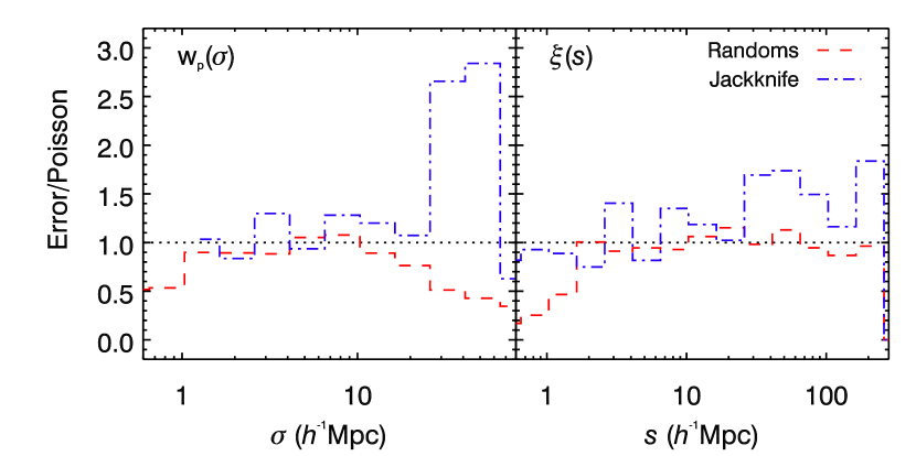
Figure 19: Ratio of the random mock (red dashed histogram) and the jack-knife (blue dot-dashed histogram) error estimates to the Poisson errors as a function of separation for the projected correlation function (left panel) and the redshift space autocorrelation function (right panel). The results are shown for the VLRS sample only.

Quantifying errors on the auto-correlation function has been performed using Poissonian, jack-knife and random realisation error estimates. The Poisson errors are given by:

$$\Delta\xi=\frac{(1+\xi)}{\sqrt{\left<DD\right>/2}}$$ (11)

The jack-knife errors were computed by splitting the data into individual fields, with the large fields (i.e. HE0940 and Q2348) being split into two fields each. We therefore have 11 different jack-knife realisations with a single field (or half-field) being excluded in each realisation.

The random realisation error estimates incorporate 100 random catalogues with the same number of objects as the real data. We then calculate the correlation function using these random realisations to calculate the $\left<DD\right>$ pairs and take the standard deviation of the results as the uncertainty on the measurement.

In Fig. 19, we compare the above error estimates for $w_{p}(\sigma)$ and the redshift space clustering function, $\xi(s)$ (see section 3.2), showing the ratio of the jack-knife and random realisation methods to the Poisson result. The estimates are consistent with each other over scales from $\approx 1-25~{}h^{-1}\mathrm{Mpc}$. In what follows, we therefore use the Poisson estimates at separations of $<25~{}h^{-1}\mathrm{Mpc}$ and jack-knife estimates at separations $>25~{}h^{-1}\mathrm{Mpc}$.

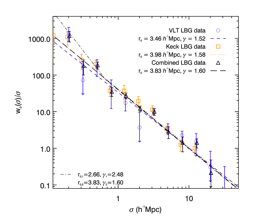
Figure 20: Projected auto-correlation function, $w_{p}(\sigma)/\sigma$, for the VLT LBG sample (black circles). The result for the $2.5<z<3.5$ Keck LBG sample is shown by the orange squares and error bars for both results are estimated using Poisson errors. The best fit power laws for both the VLT (solid black line) and Keck (dashed orange line) are shown, with clustering amplitudes of $r_{0}=3.46\pm 0.41~{}h^{-1}\mathrm{Mpc}$ and $r_{0}=3.98\pm 0.32~{}h^{-1}\mathrm{Mpc}$, with slopes of $\gamma=1.52\pm 0.13$ and $\gamma=1.58\pm 0.13$ respectively. The cyan triangles show the combined result and the dotted cyan line the best fit to this of $r_{0}=3.83\pm 0.24~{}h^{-1}\mathrm{Mpc}$ with a slope of $\gamma=1.60\pm 0.09$. The black dash-dot line shows a double power-law, motivated by Paper I, with $r_{0}=2.61~{}~{}h^{-1}\mathrm{Mpc}$ and $\gamma=2.48$ below the break and $r_{0}=3.75~{}~{}h^{-1}\mathrm{Mpc}$ and $\gamma=1.61$ above it.

The projected auto-correlation function for the VLRS sample (black circles), the Keck sample (orange squares; Steidel et al., 2003) and the two combined (cyan triangles) is shown in Fig 20. The plotted data include the integral constraint correction, which we estimated as ${\cal I}_{wp}=5.33$ and ${\cal I}_{wp}=7.18$ for the VLRS and Keck data respectively.

Based on this we estimate a clustering length of the entire VLRS sample of $r_{0}=3.46\pm 0.41~{}h^{-1}\mathrm{Mpc}$ (comoving) with a slope of $\gamma=1.52\pm 0.13$. The Keck result on it’s own gives a result of $r_{0}=3.98\pm 0.32~{}h^{-1}\mathrm{Mpc}$ with $\gamma=1.58\pm 0.13$, whilst the combined VLRS$+$Keck data gives $r_{0}=3.83\pm 0.24~{}h^{-1}\mathrm{Mpc}$ with a slope of $\gamma=1.60\pm 0.09$. These $r_{0}$ results are comparable to the clustering of star-forming galaxies at lower redshifts (e.g. Blake et al., 2009; Bielby et al., 2010).

Comparing to other measurements of the $z\approx 3$ LBG clustering length, Giavalisco & Dickinson (2001) measured $r_{0}=5.0\pm 0.7~{}h^{-1}\mathrm{Mpc}$ for $R_{AB}<25$ LBGs, but for a relatively small number of galaxies ($\approx 400$). Building on that sample, Adelberger et al. (2003) measured $r_{0}=3.96\pm 0.29~{}h^{-1}\mathrm{Mpc}$ with a slope of $\gamma=1.55\pm 0.15$ at $R_{AB}<25.5$. We note that with the same sample, but a different method, Adelberger et al. (2005b) found a higher clustering strength of $r_{0}=4.5\pm 0.6~{}h^{-1}\mathrm{Mpc}$. Subsequently, Cooke et al. (2006) measured the clustering of $z\approx 3$ LBGs in fields around damped Ly$\alpha$ absorbers and found a lower clustering strength of $r_{0}=2.65\pm 0.48~{}h^{-1}\mathrm{Mpc}$ with a slope of $\gamma=1.55\pm 0.40$ at $R_{AB}<25$, whilst Trainor & Steidel (2012) performed a similar measurement but around $z\sim 2.7$ QSOs (and with a galaxy sample incorporating a mixture of LBG and BX selections) and found a clustering length of $r_{0}=6.0\pm 0.5~{}~{}h^{-1}\mathrm{Mpc}$. Overall, our result appears consistent with other measurements, although marginally lower than the Giavalisco & Dickinson (2001); Adelberger et al. (2003, 2005b) results, which are all based on the same - or a subset of the same - sample. As observed by some of the above authors, the LBG clustering lengths are generally somewhat smaller than those measured for the slightly lower-redshift BM and BX selections.

The above estimates are based on spectroscopically confirmed samples and a number of clustering measurements exist based on photometric samples. For example Foucaud et al. (2003) measured $r_{0}=5.9\pm 0.5~{}h^{-1}\mathrm{Mpc}$ from the angular correlation function of $R_{AB}<24.5$ LBGs from the Canada-France Deep Fields Survey (McCracken et al., 2001), a higher $r_{0}$ than the spectroscopic samples, but also a significantly brighter magnitude cut. Additionally, Adelberger et al. (2005b) measured $w(\theta)$ for photometrically selected LBGs and found $r_{0}=4.0\pm 0.6~{}h^{-1}\mathrm{Mpc}$ for $R\leq 25.5$ LBGs, consistent with our results. Hildebrandt et al. (2007) measured $r_{0}=4.8\pm 0.3~{}h^{-1}\mathrm{Mpc}$ for $22.5<R_{\mathrm{Vega}}<25.5$ galaxies in the GaBoDS data. Subsequently, Hildebrandt et al. (2009) measured $r_{0}=4.25\pm 0.13~{}h^{-1}\mathrm{Mpc}$ for CFHTLS LBGs at $r_{AB}<25$ and using photo-z from HYPERZ (Bolzonella et al., 2000). In general, the clustering measured from photometric samples appears to give somewhat larger clustering lengths than those obtained for the spectroscopic samples. As with our own sample however, these selections are not perfect replicas of the original $U_{n}G\cal R$ based selection and this may be part of the cause of this, perhaps resulting in subtle differences in the redshift or luminosity ranges.

3.2 2D Auto-Correlation Function, $\xi(\sigma,\pi)$

As discussed above, integrating along the redshift/line-of-sight direction leaves the semi-projected correlation function, $w_{p}(\sigma)$, independent of the effects of galaxy peculiar motions. We now attempt to fit the full 2D correlation function, $\xi(\sigma,\pi)$, to retrieve the kinematics of the galaxy population and to make new estimates of $r_{0}$.

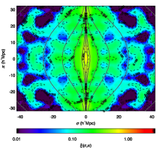
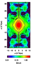
Figure 21: The two-dimensional auto-correlation function, $\xi(\sigma,\pi)$ results for the VLRS (left) and Keck (right) data samples individually. The shaded contour map and dashed contour lines show the measured $\xi(\sigma,\pi)$ in each case.

As before, we use the Landy-Szalay estimator to calculate the correlation function but now as a function of both transverse separation, $\sigma$, and line-of-sight separation, $\pi$. We use the same random catalogues matching the survey fields as used for the calculation of the projected correlation function. We again calculate the integral constraint for the data sets using the random catalogues via:

$$\frac{{\cal I}}{r_{0}^{\gamma}}=\frac{\Sigma\left<RR(s)\right>s^{\gamma}}{\Sigma\left<RR(s)\right>}$$ (12)

where $s=\sqrt{(}\sigma^{2}+\pi^{2})$. This gives values of ${\cal I}_{\xi}=0.024$ and ${\cal I}_{\xi}=0.064$ for the VLRS and Keck data samples respectively.

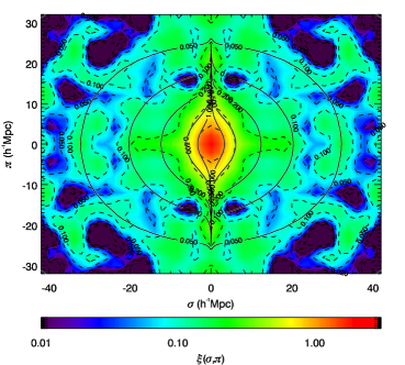
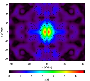
Figure 22: The two-dimensional auto-correlation function, $\xi(\sigma,\pi)$ results for the VLRS sample (left) and the signal-to-noise on the result (right). The shaded contour map and dashed contour lines show the measured $\xi(\sigma,\pi)$, whilst the solid contour lines give the best fitting model.

Fig. 21 shows the result for the VLRS data (left-hand panel), which provides a greater handle on the large scale ($s\gtrsim 10h^{-1}$Mpc) clustering, the Keck data (right panel), which provides greater sampling on small scales. Fig. 22 shows the VLRS and Keck results combined. In each case, $\xi(\sigma,\pi)$ was calculated in linear $2~{}h^{-1}\mathrm{Mpc}$ bins and subsequently smoothed with a fwhm of $2~{}h^{-1}\mathrm{Mpc}$.

For both the VLRS and Keck samples, we see the ‘finger of god’ effect at small $\sigma$ scales in which the clustering power is extended in the $\pi$ direction. This effect is a combination of galaxy peculiar velocities and measurement errors on the galaxy redshifts. In addition, in the VLRS a flattening of the clustering measurement at large scales is evident, which is caused by dynamical infall of galaxies.

We now fit models of the clustering to these results, initially assuming a single power-law for $\xi(r)$ and allowing $r_{0}$ and the kinematical parameters to vary. We take the $r_{0}$ and $\gamma$ estimates from the $w_{p}(\sigma)$ fit as the starting point in fitting the 2D clustering. The kinematics are characterised by two parameters: the velocity dispersion in the line of sight direction $\sqrt{\left<w_{z}^{2}\right>}$ and the infall parameter, $\beta$. The model we use incorporating the galaxy kinematics is described in full by Hawkins et al. (2003) and Paper I. The model accounts for two key affects on the clustering statistics caused by galaxy motions. The first is the finger-of-god effect, which is constrained by the velocity dispersion and the second is the Kaiser effect (i.e. the coherent motion of galaxies on large scales), which is characterised by $\beta$.

For the VLRS and the combined samples we fit over the range $1.0\leq s\leq 25~{}h^{-1}\mathrm{Mpc}$, whilst for the Keck data by itself we limit the fit to the scales $1.0\leq s\leq 15~{}h^{-1}\mathrm{Mpc}$ (note that the largest single field available in the Keck data is $\approx 15~{}h^{-1}\mathrm{Mpc}$).

For the two samples individually, we find that it is difficult to place reasonable constraints on both the velocity dispersion and the infall together. With the VLRS data (over the range $1\leq(\sigma,\pi)\leq 25~{}h^{-1}\mathrm{Mpc}$), we find $\beta(z=3)=0.3^{+1.7}_{-0.3}$ and $\sqrt{\left<w_{z}^{2}\right>}=1700^{+2000}_{-900}\mathrm{kms}^{-1}$, the low signal-to-noise on small scales limiting the fit accuracy. We experimented with adding a uniform error distribution out to $\pm 12000\mathrm{kms}^{-1}$ to the Gaussian velocity dispersion (c.f. Fig. 13) but this made little difference in the $\sigma,\pi$ range fitted. Fitting the Keck data gives best fit values of $\beta(z=3)=0.85^{+0.30}_{-0.35}$ and $\sqrt{\left<w_{z}^{2}\right>}=700\pm 220\mathrm{kms}^{-1}$. We note that da Ângela et al. (2005a) performed a similar fit to the Keck data for $\beta(z=3)$, but kept a constant velocity dispersion of $\sqrt{\left<w_{z}^{2}\right>}=400\mathrm{kms}^{-1}$, finding a value for the infall parameter of $\beta(z=3)=0.15^{+0.20}_{-0.15}$. By also setting the velocity dispersion to a value of $400\mathrm{kms}^{-1}$, we find that we retrieve a comparable result to da Ângela et al. (2005a), highlighting the degeneracy between the velocity dispersion and the infall parameter.

Ultimately, fitting the VLRS $\xi(\sigma,\pi)$ is hindered by a lack of signal-to-noise on small scales, whilst the fit to the Keck data is hindered by the small size of the fields. We thus combine the two datasets and fit the full LBG sample in the same manner as with the individual samples. The fit is performed in the range $1<s<25~{}h^{-1}\mathrm{Mpc}$ and we allow the velocity dispersion and the infall parameter to vary. The resulting fit gives a velocity dispersion of $\sqrt{\left<w_{z}^{2}\right>}=420^{+140}_{-160}\mathrm{kms}^{-1}$ and an infall parameter of $\beta(z=3)=0.38\pm 0.19$. We show the $\chi^{2}$ contours for the fit in the $\beta(z=3)-\sqrt{\left<w_{z}^{2}\right>}$ plane in Fig. 23 (the contours represent the $1\sigma$, $2\sigma$ and $3\sigma$ confidence limits). From this figure, the degeneracy can be seen between $\sqrt{\left<w_{z}^{2}\right>}$ and $\beta$, where increasing $\beta$ similarly increases the best fit velocity dispersion. The best fitting results are plotted over the contour maps of the $\xi(\sigma,\pi)$ measurements in Fig. 22 (dashed contours). As with the data, we see the finger-of-god and large scale flattening effects in the fitted models.

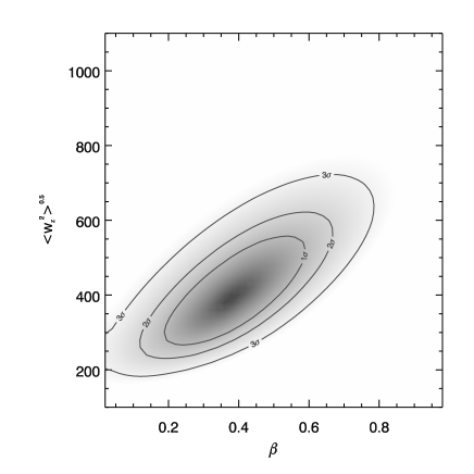
Figure 23: Fitting contours for peculiar velocity and bulk inflow based on the combined VLRS$+$Keck $\xi(\sigma,\pi)$. The best fitting result is given by $\beta(z=3)=0.38\pm 0.19$ and $\sqrt{\left<w_{z}^{2}\right>}=420^{+140}_{-160}\mathrm{kms}^{-1}$.

3.3 Redshift-space correlation function, $\xi(s)$.

In order to check the consistency of our measurements, we now compare the model fit obtained from $w_{p}(\sigma)$ and $\xi(\sigma,\pi)$ to the measured redshift-space auto-correlation function $\xi(s)$. Again we use the Landy-Szalay estimator and quote errors based on Poisson estimates. The $\xi(s)$ results for the VLRS, Keck and combined LBG samples are shown in Fig. 24. We also plot the single power law estimate of the intrinsic clustering from our fits to the VLT$+$Keck $\xi(\sigma,\pi)$ (dotted line) and the result of this power-law after applying the best fit values for $\beta$ and $\sqrt{\left<w_{z}^{2}\right>}$ (dashed line). The final fit incorporating the galaxy dynamics is marginally low compared to the data-points, but is easily consistent within the error bars.

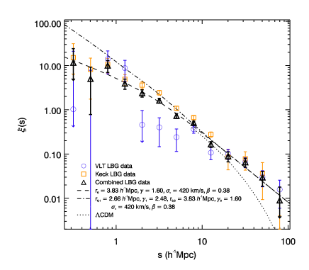
Figure 24: Redshift space correlation function, $\xi(s)$, for the VLRS (open blue circles), Keck (orange squares) and combined (black triangles) samples. The short and long dashed curves show single power law model fits to the combined sample based on fits to $w_{p}(\sigma)$ and $\xi(\sigma,\pi)$. The dash-dot curve gives a double power law model fit, whilst the dotted curve at large scales shows the predicted $\Lambda$CDM clustering.

Our measurements of $\beta$ and $\sqrt{\left<w_{z}^{2}\right>}$ are consistent with the previous measurements using the first VLT dataset ( Paper I, $\beta=0.48$ and $\sqrt{\left<w_{z}^{2}\right>}=700~{}\mathrm{kms}^{-1}$). As discussed in Paper I, the median measurement error on the galaxy lines on the VLT VIMOS spectra is $\approx 350\mathrm{kms}^{-1}$. In addition, an uncertainty of $\approx 100\mathrm{kms}^{-1}$ is introduced by the transformation from outflow redshifts to intrinsic galaxy redshifts (Steidel et al., 2010). The final contribution to the velocity dispersion is from the intrinsic peculiar velocities of the galaxies. Using the GIMIC simulations (Crain et al., 2009) we have analysed the mean velocity dispersion of LBG-like galaxies and find a value of $\approx 100\mathrm{kms}^{-1}$. Combining these three elements in quadrature, we would expect a pairwise velocity dispersion of $\sqrt{\left<w_{z}^{2}\right>}\approx\sqrt{2}\times\sqrt{(350\mathrm{kms}^{-1})^{2}+(100\mathrm{kms}^{-1})^{2}+(100\mathrm{kms}^{-1})^{2}}\approx 500\mathrm{kms}^{-1}$. This is within the $1\sigma$ error contours given in Fig. 23. This value is also reasonably consistent with the VLRS $\xi(s)$ estimate (see Fig. 24).

We also show in Fig. 24 the matter correlation, $\xi(r)$, scaled to the LBG clustering strength. This was calculated using the CAMB software and using a flat $\Lambda$CDM cosmology with $\Omega_{m}=0.27$, $H_{0}=70\mathrm{kms}^{-1}$Mpc^-1 and $\Omega_{b}h^{2}=0.022$. There are currently some claims that non-Gaussianity is detected at $z\approx 1$ in NRAO VLA Sky Survey radio source (Xia et al., 2010) and Luminous Red Galaxy (LRG) datasets (Thomas et al., 2011; Sawangwit et al., 2011; Nikoloudakis et al., 2012). The evidence generally comes comes from detecting large scale excess power via flatter slopes for angular correlation functions. Since non-Gaussianity is easier to detect at high redshift this motivates checking the LBG $\xi(s)$ for an excess. We have already noted that the slope from $w_{p}$ and $\xi(\sigma,\pi)$ at $\gamma=1.55$ is much flatter than the canonical $\gamma=1.8$. This slope is also flatter than the $z\approx 1$ LRG large-scale $w(\theta)$ slope of Nikoloudakis et al. (2012). We see that the VLRS does give reasonably accurate measurements for $25<s<100~{}h^{-1}\mathrm{Mpc}$ and that the observed LBG $\xi(s)$ shows a $\approx 2.5\sigma$ excess over the $\Lambda$CDM model in this range. Even when the marginally smaller integral constraint for the $\Lambda$CDM model is assumed the discrepancy remains at $\approx 2\sigma$. We conclude that there is some evidence for an excess over the standard $\Lambda$CDM model but independent LBG data is needed to confirm this on the basis of the redshift space correlation function. The statistical error on the LBG $w(\theta)$ from Paper I is smaller but the flat power-law here is only seen to $\theta=10^{\prime}$ or $r=13-14~{}h^{-1}\mathrm{Mpc}$ and this is not enough to decide the issue.

3.4 Double power-law correlation function models

We next look to see if a more complicated model than a power-law for $\xi(r)$ is required. This is motivated firstly because Paper I noted that there was an increase in the slope at $\approx 1~{}h^{-1}\mathrm{Mpc}$ in the LBG angular auto-correlation function, $w(\theta)$, suggestive of the split between the 1-halo and 2-halo terms in the halo model of clustering. Although this result is uncertain due to quite significant low redshift contamination corrections, such features have been seen in lower redshift galaxy samples, particularly for LRGs at $z\approx 0.5$ (e.g. Ross et al., 2007; Sawangwit et al., 2011). Given the improved power of the VLRS, it is interesting to see if there is any evidence of a change in the slope at small scales in $\xi(s)$ and $w_{p}(\sigma)$ in our $z\approx 3$ LBG sample.

We therefore show in Fig. 20 a double power-law model for $w_{p}$ with the same power-law slopes as fitted by Paper I to the LBG $w(\theta)$. We have reduced the amplitude by $\approx 20\%$ to match approximately the large-scale amplitude fitted to the VLRS and Keck combined data. This is within the systematic uncertainties of the $w(\theta)$ measurement. Although certainly not required by the $w_{p}$ data this double power-law cannot be rejected by the combined $w_{p}$ data, giving a reduced $\chi^{2}$ of 1.77 (marginally smaller than the reduced $\chi^{2}$ obtained for a single power law of 1.84).

In Fig. 24 we now compare to $\xi(s)$ the same double power-law $w(\theta)$ model with the $\approx 20\%$ reduced amplitude. Again with a velocity dispersion of $420\mathrm{kms}^{-1}$ and $\beta=0.38$ we see that the model cannot be rejected by the data. We note that if we use a $\left<DD\right>/\left<DR\right>$ estimator the VLRS $\xi(s)$ result shows increased power at large scales and the flatter slope of the double power-law model here provides a better fit.

We note that other authors have also reported a turn-up in the clustering at small scales in high redshift galaxy samples. For instance Ouchi et al. (2005) reports that $z=4$ LBG $w(\theta)$ shows a steepening below $\approx 0.2~{}h^{-1}\mathrm{Mpc}$ or $\approx 10^{\prime\prime}$ at $z=4$. If both results are unaffected by contamination then it could argue for an evolutionary growth in this break scale between $z=4$ and $z=3$.

Certainly there is plenty to motivate expanding surveys to make more accurate measurements of both the angular and redshift survey correlation functions at these redshifts. Below the break scale is of extreme interest for single halo galaxy formation models and at large scales the interest is in looking for a flattening of the correlation function slope due to the presence of primordial non-Gaussianity.

3.5 Estimating $\Omega_{m}$ and the growth rate

3.5.1 The mass density of the Universe

We now look at the cosmological results afforded by the $z\approx 3$ LBG clustering and dynamics. As discussed by Hoyle et al. (2002); da Ângela et al. (2005b), it is, in principle, possible to constrain the matter density $\Omega_{m}(z=0)$ from the measurement of $\xi(\sigma,\pi)$. Effectively, the elongation of $\xi(\sigma,\pi)$ along the line of sight increases with increasing values of $\Omega_{m}(z=0)$. However, increased values of $\beta$ lead to a flattening of $\xi(\sigma,\pi)$ along the line of sight. These effects combined lead to a degeneracy in determining $\Omega_{m}$ from the galaxy clustering alone.

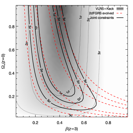
Figure 25: Fitting contours for the mass density and bulk inflow based on the combined VLRS$+$Keck $\xi(\sigma,\pi)$. The shaded region gives the result from the VLT$+$Keck data sample (assuming $\sqrt{\left<w_{z}^{2}\right>}=420\mathrm{kms}^{-1}$, $r_{0}=3.83~{}h^{-1}\mathrm{Mpc}$ and $\gamma=1.60$) with the dotted contour lines giving the 1, 2 and $3\sigma$ uncertainties. The results from this fit are $\beta(z=3)=0.38^{+0.15}_{-0.13}$ and $\Omega_{m}(z=0)=0.08^{+0.22}_{-0.08}$. The dashed red lines show the 1, 2 and $3\sigma$ constraints given by evolving the 2dFGRS measurements as described in the text. The solid black contours give the combination of the two and give a result of $\beta(z=3)=0.38^{+0.16}_{-0.09}$ and $\Omega_{m}(z=0)=0.30^{+0.32}_{-0.18}$.

In previous sections, we have studied the galaxy dynamics assuming a cosmology with $\Omega_{m}(z=0)=0.3$. We now fit the $\xi(\sigma,\pi)$ result with this assumed cosmology, but now with a constant peculiar velocity of $\sqrt{\left<w_{z}^{2}\right>}=420\mathrm{kms}^{-1}$ and fitting for $\Omega_{m}(z=0)$ and $\beta$. The result is shown by the $1\sigma$, $2\sigma$ and $3\sigma$ contours (solid) in Fig. 25. Based on just the $z=3$ galaxy clustering, we find results for the mass density of $\Omega_{m}(z=0)=0.08^{+0.22}_{-0.08}$ and on the infall parameter of $\beta(z=3)=0.38^{+0.15}_{-0.13}$.

Breaking the degeneracy of this result can be achieved by incorporating lower redshift results as shown by da Ângela et al. (2005a, b) and Paper I. As in these previous works, we use the 2dFGRS measurements of Hawkins et al. (2003) to do this ($r_{0}=5.0~{}h^{-1}\mathrm{Mpc}$, $\gamma=1.8$ and $\beta(z=0.11)=0.49\pm 0.09$). The Hawkins et al. (2003) result can then be evolved to the redshift of our study based on the relationship between the growth parameter, $f(z)$, and the bulk motion and the clustering bias, $b$, of a galaxy population:

$$\beta=\frac{f(z)}{b}\approx\frac{\Omega_{m}(z)^{0.55}}{b}$$ (13)

The bias can be calculated directly from the clustering measurements by using the volume averaged clustering:

$$b=\sqrt{\frac{\xi_{g}(s)}{\xi_{DM}(s)}}=\sqrt{\frac{\overset{\_}{\xi}_{g}(8)}{\overset{\_}{\xi}_{DM}(8)}}$$ (14)

where $\overset{\_}{\xi}_{g}(8)$ is the volume averaged correlation function at $s<8~{}h^{-1}\mathrm{Mpc}$ for the galaxy population and $\overset{\_}{\xi}_{DM}(8)$ is the same, but for the underlying dark matter distribution. The volume averaged clustering is calculated from the clustering using:

$$\overset{\_}{\xi}(x)=\frac{3}{x^{3}}\int^{x}_{0}r^{2}\xi(r)\mbox{d}r$$ (15)

In addition, a measure of the dark matter clustering is required in order to estimate the bias of the galaxy population and we calculate this using the CAMB software incorporating the HALOFIT model of non-linearities (Smith et al., 2003). Using the previously determined best fit parameters of $r_{0}=3.83~{}h^{-1}\mathrm{Mpc}$ and $\gamma=1.60$, we evaluate the galaxy bias based on a single power-law, finding a bias for the LBGs of $b=2.59\pm 0.13$.

We then determine the $z=0.11$ underlying dark matter clustering amplitude from these parameter constraints and evolve this to $z=3$ for test cosmology range of $\Omega_{m}(z=0)=0-1$. The constraints on $\beta$ using this method over a range of assumed $\Omega_{m}$ values are given by the red dashed contours in Fig 25. By combining these with the original constraints from $\xi(\sigma,\pi)$, we find a result of $\beta(z=3)=0.38^{+0.16}_{-0.09}$ and $\Omega_{m}(z=0)=0.30^{+0.32}_{-0.18}$.

Across these analyses, we have consistently found a value for the infall parameter of $\beta(z=3)\approx 0.36-0.40$. $\Omega_{m}$ is somewhat less well constrained, but remains consistent with $\Lambda$CDM. The measurements of $\beta(z=3)$ presented here are consistent with our previous measurement from Paper I of $\beta(z=3)=0.48\pm 0.17$, whilst being somewhat higher than the result found by da Ângela et al. (2005a) of $\beta(z=3)=0.15^{+0.20}_{-0.15}$. We note that the latter assumes a fixed velocity dispersion of $\sqrt{\left<w_{z}^{2}\right>}=400\mathrm{kms}^{-1}$ and is limited to the small field of view of the Keck survey As such, their lower estimate of $\beta$ may well be a systematic of too small an area to identify the Kaiser effect as well as not being able to simultaneously fit for the velocity dispersion.

3.5.2 Growth rate results compared

Using the results for $\beta$ and the galaxy bias we can compare our constraints of the growth parameter $f(z)$ to previous results. Guzzo et al. (2008) presented the results of such an analysis based on the VLT VIMOS Deep Survey (VVDS), showing values for $f(z)$ extracted from a number of galaxy surveys up to a redshift of $z\approx 0.8$. Here we add the $z\approx 3$ result from our survey. We present measurements in terms of both $f(z)$ and $f\sigma_{8}$, where $f\sigma_{8}$ is intended to give a measurement which is less dependent on the cosmology assumed for the calculation of the clustering (e.g. Song & Percival, 2009).

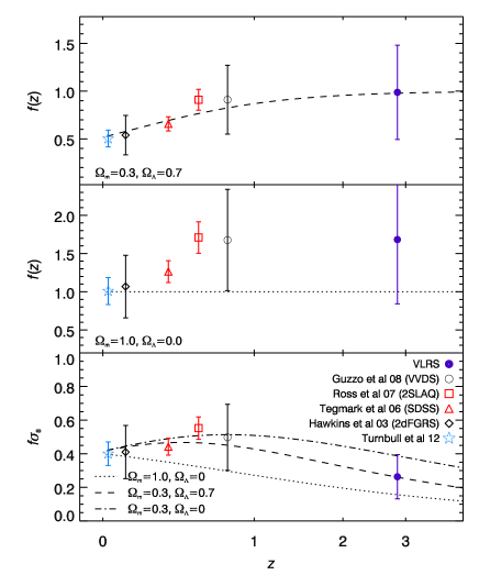
Figure 26: The evolution of the growth factor based on available $z<1$ survey observations and the constraint from the VLRS data (solid blue circle).

We have already calculated the infall parameter and take the value ($\beta=0.38$) obtained via fitting the velocity dispersion and $\beta$ in a $\Lambda$CDM cosmology with $\Omega_{m}=0.3$ and $\Omega_{\Lambda}=0.7$ (Fig. 23). Combining this with our measurement of the galaxy bias gives a value for the growth parameter based on the combined LBG sample of $f(z=3)=0.99\pm 0.50$.

We present the $f(z=3)$ result (filled blue circle) in the top panel of Fig. 26 alongside a number of other low-redshift measurements. In order of ascending redshift, the star shows the measurement of Turnbull et al. (2012) based on local supernovae measurements, the diamond shows the result based on the 2dFGRS presented by Hawkins et al. (2003), the red triangle shows the SDSS result based on LRGs from Tegmark et al. (2006), the red square shows the 2SLAQ result also estimated from the LRG population of Ross et al. (2007) and the black circle shows the VVDS result of Guzzo et al. (2008). For completeness these are also summarised in Table 12.

Table 12: Summary of growth parameter results from the literature.

[b] Survey $z$ $b$ $\beta$ $f$ $f\sigma_{8}$ First Amendment SNe 0.025 — —- — $0.40\pm 0.07$ 2dFGRS² 0.11 $1.15\pm 0.06$ $0.47\pm 0.18$ $0.54\pm 0.21$ $0.41\pm 0.16$ SDSS LRGs 0.35 $2.13$ $0.31\pm 0.04$ $0.66\pm 0.07$ $0.44\pm 0.05$ 2SLAQ LRGs 0.55 $2.02\pm 0.10$ $0.45\pm 0.05$ $0.91\pm 0.11$ $0.55\pm 0.07$ VVDS 0.77 $1.30\pm 0.10$ $0.70\pm 0.26$ $0.91\pm 0.07$ $0.50\pm 0.04$ VLRS$+$Keck 2.85 $2.59\pm 0.13$ $0.38\pm 0.19$ $0.99\pm 0.50$ $0.26\pm 0.13$

• Turnbull et al. (2012)

• Hawkins et al. (2003)

• Tegmark et al. (2006)

• Song & Percival (2009)

• Ross et al. (2007)

• Guzzo et al. (2008)

In the middle panel of Fig. 26, we also plot the evolution of $f(z)$ based on the assumed $\Lambda$CDM cosmology (dashed line), where $f(z)=\Omega_{m}(z)^{0.55}$. The low redshift data points are all consistent with the assumed cosmology at the $\sim 1\sigma$ level and at $z=3$, the model cosmology is again consistent with the data. We note again that the observations themselves depend on the assumed cosmology via $\sigma_{8}(z)$ and so to test the $\Omega_{m}=1$ cosmology we adjust the observed values of $f(z)$ for the effects of different cosmology in eq. 14 according to the methods set out by da Ângela et al. (2005a). Also assuming that $\beta$ is approximately independent of the assumed cosmology, we see that the $\Omega_{m}=1$ $z$-independent growth rate is apparently rejected by the data. However, if the bias is allowed to float rather than just fit the lowest redshift point then the model may only be rejected at the $1-2\sigma$ level, consistent with the conclusions from Fig. 25.

If we now consider $f\sigma_{8}$, the observations are now independent of the assumed cosmology, at least given again the assumption that the observed $\beta$ is approximately cosmology indpendent. Each of the observational measurements is again plotted in the top panel of Fig. 26, but now in terms of $f\sigma_{8}$. We now plot three test cosmologies for comparison, the $\Lambda$CDM used in the top panel (dashed line), plus an Einstein-de-Sitter model ($\Omega_{m}=1$, $\Omega_{\Lambda}=0$, dotted line) and an open Universe without a cosmological constant and a mass density of $\Omega_{m}=0.3$ (dot-dash line). For each model we incorporate a factor ($c_{at}$) to correct for the cosmology assumed in the measurement of the clustering observations being different from the test cosmology. Each model is thus given by:

$$(f\sigma_{8})_{a}=\beta\sigma_{g,a}=\frac{\beta\sigma_{g,t}}{\sqrt{c_{at}}}=\frac{(f\sigma_{8})_{t}}{\sqrt{c_{at}}}=\frac{\Omega_{m,t}(z)^{0.55}\sigma_{8,t}(z)}{\sqrt{c_{at}(z)}}$$ (16)

where an index of $t$ denotes a parameter calculated in the test cosmology and an index of $a$ denotes a parameter calculated in the assumed cosmology (i.e. $\Lambda$CDM). We normalise $\sigma_{8}$ to 0.8 at $z=0$ and $\sigma_{g}$ is effectively $\sigma_{8}$ measured for the galaxy population. If we assume a power-law form for the clustering with a slope of $\gamma=1.8$, then following Ballinger et al. (1996); da Ângela et al. (2005a) $c_{at}$ is given by:

$$c_{at}=\left(\left(\frac{B_{t}}{B_{a}}\right)^{2}\frac{A_{t}}{A_{a}}\right)^{2/3}$$ (17)

with $A$ and $B$ (da Ângela et al., 2005a) given by:

$$A=\frac{c}{H_{0}}\frac{1}{\Omega_{\Lambda}^{0}+\Omega_{m}^{0}(1+z)^{3}}$$ (18)

$$B=\frac{c}{H_{0}}\int_{0}^{z}\frac{\mbox{d}z^{\prime}}{\Omega_{\Lambda}^{0}+\Omega_{m}^{0}(1+z^{\prime})^{3}}$$ (19)

We are assuming here that $\beta$ is independent of cosmology, a reasonable approximation when $\Omega_{m}\ga 0.1$

With the models corrected to account for differences between the cosmology assumed for the observations and the model cosmologies, the observations now provide clearer tests on the models. We note that the observations (excepting the SDSS point) assume the $\Omega_{m}=0.3$/$\Omega_{\Lambda}=0.7$ cosmology and so there is no change in the relationship between the observations and the $\Lambda$CDM model between the top and bottom panels. Thus the VLRS datapoint shows the same level of consistency with the $\Lambda$CDM model for $f\sigma_{8}$ and $f(z)$.

At redshifts of $z<1$, we see that flat and open cosmologies (i.e. with and without a cosmological constant) are poorly distinguished by the available observations. At $z=3$, we find that the VLRS data can only reject the open cosmology with $\Omega_{m}=0.3$ at the $\approx 1\sigma$ level. The Einstein-de Sitter cosmology is apparently rejected by combining the $z<1$ and $z\approx 3$ observations. But again if the normalisation of the model is allowed to float rather than be fixed on the low-redshift SNe observation, the model still fits the data with a reduced $\chi^{2}$ of 2.7.

3.6 The dark matter halos of $z\sim 3$ star-forming galaxies

We now look at the nature of the halos that host the LBG sample based on our clustering results using the halo-occupation distribution (HOD) model formalism (e.g. Ma & Fry, 2000; Peacock & Smith, 2000; Zehavi et al., 2004; Zheng et al., 2005). By matching our clustering results to the measured clustering properties of simulated dark matter halos, we estimate mean halo masses ($\left<M_{h}\right>$), minimum halo masses ($M_{min}$) and cumulative occupation numbers ($\left<N(M)\right>$) for the VLRS, Keck and combined samples. The simulation results are obtained from the cosmological dark matter simulation described by González & Padilla (2010) and the results are given in Table 13.

Table 13: Results of the halo matching analysis.

Sample	Bias	log($\left<M_{h}\right>$/$h^{-1}$M⊙)	log($M_{min}$/$h^{-1}$M⊙)	$\left<N(M)\right>$
VLRS	$2.37\pm 0.21$	$11.57\pm 0.15$	$11.13\pm 0.18$	$1.2\pm 0.6$
Keck	$2.78\pm 0.13$	$11.69\pm 0.10$	$11.30\pm 0.10$	$1.8\pm 0.6$
Combined	$2.59\pm 0.13$	$11.73\pm 0.07$	$11.33\pm 0.09$	$2.0\pm 0.5$

We find that the results are consistent within the error bars between the VLRS and Keck samples evaluated separately, with mean host halo masses of $\sim 10^{1}1.6~{}h^{-1}$M_⊙. This lends additional credence to our having combined the two samples in order to improve the statistical fidelity of the 2D clustering results. In addition we note that the occupation numbers suggest that multiple LBGs are present in single galaxies, with $\left<N(M)\right>$ consistently $>1$ for all the samples although this is with relatively large uncertainties.

There are few other measurements of the halo masses of $z\sim 3$ LBGs available in the literature that are based on spectroscopic data. In terms of photometric samples, Foucaud et al. (2003), Hildebrandt et al. (2007) and Yoshida et al. (2008) measure halo masses of bright $z\approx 3$ LBG samples of $M_{DM}\sim 10^{12}h^{-1}\rm{M_{\odot}}$, an order of magnitude larger than for our sample. However, in a similarly photometric study, Lee et al. (2006) found marginally lower halo masses of $\sim 5-10\times 10^{11}h^{-1}\rm{M_{\odot}}$ for both $z\sim 3$ and $z\sim 4$ LBGs, the $z\sim 3$ LBGs having a magnitude limit of $r=25.5$. Similarly, the results of Trainor & Steidel (2012) show a halo mass of $M_{DM}\sim 10^{11.9\pm 0.1}h^{-1}\rm{M_{\odot}}$, but is based on galaxies with a redshift distribution somewhat lower than our own.

In terms of the spectroscopic samples closest in redshift and form to our own, work using the Steidel et al. (2003, 2004) data report halo masses of $M_{DM}\sim 10^{11.5\pm 0.3}h^{-1}\rm{M_{\odot}}$ (Adelberger et al., 2005b). These spectroscopic $z\sim 3$ based measurements are in good agreement with our own results. This is as one would expect for our ‘Keck’ sample given that this uses some of the same data as the above results, whilst the consistency between these results and the result from our own pure-VLRS sample adds weight to the results as a whole. As noted by previous authors, the LBG host halo masses are approximately an order of magnitude lower than those measured for the infrared selected population at $z\sim 3$ (e.g. Quadri et al., 2007), hinting at the continued trend for a ‘blue’ star-forming population existing in low-density environments and a ‘red’, potentially more passive population inhabiting denser environments.

4 Conclusions

We have presented the widest area spectroscopic survey of galaxies thus far in the redshift range $2<z<3.5$, based on observations with the VLT VIMOS instrument. This paper adds to the initial dataset of Bielby et al. (2011), where data in five 0.5^∘ $\times$ 0.5^∘ fields were presented. Here we add a further four new fields, each with deep optical imaging over an area of $\approx$ 0.5^∘$\times$ 0.5^∘ in three cases and a full 1^∘ $\times$ 1^∘ in the fourth field. In addition, we have extended one of the original fields of Paper I to 1^∘$\times$ 1^∘ from the original 0.5^∘ $\times$ 0.5^∘. In total therefore, we now have $\approx 4$ deg² of optical imaging with a minimum of three bands in each field incorporating $U$, $B$ and $R$ or equivalents.

In total, the survey now consists of 1,994 spectroscopically confirmed $z>2$ galaxies. The properties of the full sample have been presented here with redshift and magnitude distributions as well as example and composite spectra. The mean redshift of our $z>2$ galaxy dataset is $\bar{z}=2.79$. In addition, we detect 30 AGN or quasars, $\approx 800$ low-redshift galaxies and $\approx$130 Galactic stars. Using the $z>2$ galaxy dataset, we have conducted an analysis of the galaxy clustering at $z\sim 3$. Using the semi-projected correlation function, we have measured a galaxy clustering length of $r_{0}=3.46\pm 0.41~{}h^{-1}\mathrm{Mpc}$ with a slope of $\gamma=1.52\pm 0.26$, assuming a power-law form to $\xi(r)$. We have also combined the VLRS sample with the Keck LBG sample of Steidel et al. (2003), which provides greater statistical power on small scales (i.e. $s\lesssim 2~{}h^{-1}\mathrm{Mpc}$) than the VLRS but does not provide the coverage of the VLRS at larger scales (i.e. $s\gtrsim 8~{}h^{-1}\mathrm{Mpc}$). For the combined sample we measure a clustering length of $r_{0}=3.83\pm 0.24~{}h^{-1}\mathrm{Mpc}$, with a slope of $\gamma=1.60\pm 0.09$.

We have shown that the LBG correlation functions consistently show slopes that are significantly flatter than the canonical $\gamma=1.8$ observed at low redshift. Indeed, the measured slopes of $\gamma=1.55$ are flatter than in some $z\approx 1$ galaxy and radio-source correlation functions that have been interpreted as showing evidence for primordial non-Gaussianity (Xia et al., 2010; Thomas et al., 2011; Sawangwit et al., 2011; Nikoloudakis et al., 2012). Non-Gaussianity is expected to be easier to detect at large-scales and high redshift. We have therefore checked whether a standard $\Lambda$CDM model is consistent with the form of the VLRS $\xi(s)$ in particular in the regime $10<s<50~{}h^{-1}\mathrm{Mpc}$. We found that there is evidence that the LBGs are showing more large-scale power than the standard model in this regime but only at $\approx 2\sigma$. More studies of LBG clustering at large-scales are clearly needed to check these results.

In addition to the 1D clustering analyses, we have also investigated the 2D correlation function and the imprints of galaxy dynamics on the clustering. We find that the 2D clustering for the VLRS$+$Keck LBG sample is well fit by a model based on a power-law fit with a clustering length of $r_{0}=3.46~{}h^{-1}\mathrm{Mpc}$, a large scale infall parameter of $\beta=0.38\pm 0.19$ and a velocity dispersion of $\sqrt{\left<w_{z}^{2}\right>}=420^{+140}_{-160}\mathrm{kms}^{-1}$, over a range of $1<s<25~{}h^{-1}\mathrm{Mpc}$. We have shown that this result is consistent with the model for the redshift space correlation function, $\xi(s)$, measured for the combined sample.

We use the 2D galaxy clustering results to determine the matter density parameter and the growth parameter. Using the previously constrained form for the clustering and galaxy velocity dispersion, we fit the 2D correlation function for the matter density, $\Omega_{m}$. We find an acceptable range in the matter density of $\Omega_{m}(z=0)=0.08^{+0.22}_{-0.08}$ (with an infall parameter of $\beta(z=3)=0.38^{+0.15}_{-0.13}$). We add a further constraint provided by the 2dFGRS low-redshift clustering measurements, which gives $\Omega_{m}(z=0)=0.30^{+0.32}_{-0.18}$ (with an infall parameter of $\beta(z=3)=0.38^{+0.16}_{-0.09}$). Although the constraints on the mass density are relatively weak, we see that the constraints on the infall parameter remain consistent. Using these measurements to constrain the growth parameter, we find a value of $f(z=3)=b\beta=0.99\pm 0.50$. In addition we determine the combined parameter $f\sigma_{8}$, which gives a measure of the growth parameter that is less dependent on the assumed underlying dark matter mass distribution. In this case we find a value of $f\sigma_{8}=0.26\pm 0.13$. These measurements are the highest redshift constraint on the growth parameter based on galaxy clustering analyses. We have shown that these measurements are consistent with the $\Lambda$CDM standard model, although given the uncertainties on the measurements, they are also consistent with a number of other cosmologies.

Based on the clustering results, we estimate typical halo masses for the dark matter halos that host the LBG population. For the VLRS sample alone, we estimate a mean halo mass of $M_{DM}=10^{11.57\pm 0.15}$, consistent with measurements based on comparable spectroscopic LBG samples at $z\sim 3$ and an order of magnitude lower than the typical halo masses hosting $z\sim 3$ infra-red selected galaxies.

This work is one of the largest surveys of the galaxy mass distribution at $z\approx 3$ and paves the way for a number of lines of research, which will be followed in subsequent papers. In particular, the proximity of the data presented here to quasar sightlines will provide important constraints on the relationship between galaxies and the IGM at an epoch associated with significant interactions between the two.

References

- Adelberger et al. (2005a) Adelberger K. L., Shapley A. E., Steidel C. C., Pettini M., Erb D. K., Reddy N. A.,. 2005a, ApJ, 629, 636
- Adelberger et al. (2005b) Adelberger K. L., Steidel C. C., Pettini M., Shapley A. E., Reddy N. A., Erb D. K.,. 2005b, ApJ, 619, 697
- Adelberger et al. (2004) Adelberger K. L., Steidel C. C., Shapley A. E., Hunt M. P., Erb D. K., Reddy N. A., Pettini M.,. 2004, ApJ, 607, 226
- Adelberger et al. (2003) Adelberger K. L., Steidel C. C., Shapley A. E., Pettini M.,. 2003, ApJ, 584, 45
- Ballinger et al. (1996) Ballinger W. E., Peacock J. A., Heavens A. F.,. 1996, MNRAS, 282, 877
- Baugh et al. (1996) Baugh C. M., Gardner J. P., Frenk C. S., Sharples R. M.,. 1996, MNRAS, 283, L15
- Bertin (2006) Bertin E.,. 2006, in Astronomical Society of the Pacific Conference Series, Vol. 351, Astronomical Data Analysis Software and Systems XV, ed. C. Gabriel, C. Arviset, D. Ponz, & S. Enrique, 112–+
- Bertin et al. (2002) Bertin E., Mellier Y., Radovich M., Missonnier G., Didelon P., Morin B.,. 2002, in Astronomical Society of the Pacific Conference Series, Vol. 281, Astronomical Data Analysis Software and Systems XI, ed. D. A. Bohlender, D. Durand,,T. H. Handley, 228–+
- Bielby et al. (2010) Bielby R., Shanks T., Sawangwit U., Croom S. M., Ross N. P., Wake D. A.,. 2010, MNRAS, 403, 1261
- Bielby et al. (2011) Bielby R. M., et al. . 2011, MNRAS, 414, 2
- Blake et al. (2009) Blake C., et al. . 2009, MNRAS, 395, 240
- Bolzonella et al. (2000) Bolzonella M., Miralles J., Pelló R.,. 2000, A&A, 363, 476
- Conroy et al. (2008) Conroy C., Shapley A. E., Tinker J. L., Santos M. R., Lemson G.,. 2008, ApJ, 679, 1192
- Cooke et al. (2006) Cooke J., Wolfe A. M., Gawiser E., Prochaska J. X.,. 2006, ApJ, 652, 994
- Cowie & Hu (1998) Cowie L. L., Hu E. M.,. 1998, AJ, 115, 1319
- Crain et al. (2009) Crain R. A., et al. . 2009, MNRAS, 399, 1773
- Crighton et al. (2011) Crighton N. H. M., et al. . 2011, MNRAS, 414, 28
- da Ângela et al. (2005a) da Ângela J., Outram P. J., Shanks T.,. 2005a, MNRAS, 361, 879
- da Ângela et al. (2005b) da Ângela J., Outram P. J., Shanks T., Boyle B. J., Croom S. M., Loaring N. S., Miller L., Smith R. J.,. 2005b, MNRAS, 360, 1040
- Foucaud et al. (2003) Foucaud S., McCracken H. J., Le Fèvre O., Arnouts S., Brodwin M., Lilly S. J., Crampton D., Mellier Y.,. 2003, A&A, 409, 835
- Fukugita et al. (1996) Fukugita M., Ichikawa T., Gunn J. E., Doi M., Shimasaku K., Schneider D. P.,. 1996, AJ, 111, 1748
- Gawiser et al. (2007) Gawiser E., et al. . 2007, ApJ, 671, 278
- Gawiser et al. (2006) Gawiser E., et al. . 2006, ApJ, 642, L13
- Giavalisco & Dickinson (2001) Giavalisco M., Dickinson M.,. 2001, ApJ, 550, 177
- González et al. (2012) González J. E., Lacey C. G., Baugh C. M., Frenk C. S., Benson A. J.,. 2012, MNRAS, 423, 3709
- González & Padilla (2010) González R. E., Padilla N. D.,. 2010, MNRAS, 407, 1449
- Groth & Peebles (1977) Groth E. J., Peebles P. J. E.,. 1977, ApJ, 217, 385
- Guzzo et al. (2008) Guzzo L., et al. . 2008, Nature, 451, 541
- Hainline et al. (2011) Hainline K. N., Shapley A. E., Greene J. E., Steidel C. C.,. 2011, ApJ, 733, 31
- Hainline et al. (2012) Hainline K. N., Shapley A. E., Greene J. E., Steidel C. C., Reddy N. A., Erb D. K.,. 2012, ArXiv e-prints
- Hawkins et al. (2003) Hawkins E., et al. . 2003, MNRAS, 346, 78
- Hildebrandt et al. (2012) Hildebrandt H., et al. . 2012, MNRAS, 2386
- Hildebrandt et al. (2007) Hildebrandt H., Pielorz J., Erben T., Schneider P., Eifler T., Simon P., Dietrich J. P.,. 2007, A&A, 462, 865
- Hildebrandt et al. (2009) Hildebrandt H., Pielorz J., Erben T., van Waerbeke L., Simon P., Capak P.,. 2009, A&A, 498, 725
- Hoyle et al. (2002) Hoyle F., Outram P. J., Shanks T., Boyle B. J., Croom S. M., Smith R. J.,. 2002, MNRAS, 332, 311
- Jenkins et al. (1998) Jenkins A., et al. . 1998, ApJ, 499, 20
- Jose et al. (2012) Jose C., Subramanian K., Srianand R., Samui S.,. 2012, ArXiv e-prints
- Kim et al. (2009) Kim H., Baugh C. M., Cole S., Frenk C. S., Benson A. J.,. 2009, MNRAS, 400, 1527
- Le Fèvre et al. (2003) Le Fèvre O., et al. . 2003, in Society of Photo-Optical Instrumentation Engineers (SPIE) Conference Series, Vol. 4841, Society of Photo-Optical Instrumentation Engineers (SPIE) Conference Series, ed. M. Iye & A. F. M. Moorwood, 1670–1681
- Lee et al. (2006) Lee K.-S., Giavalisco M., Gnedin O. Y., Somerville R. S., Ferguson H. C., Dickinson M., Ouchi M.,. 2006, ApJ, 642, 63
- Ma & Fry (2000) Ma C.-P., Fry J. N.,. 2000, ApJ, 543, 503
- Madau et al. (1996) Madau P., Ferguson H. C., Dickinson M. E., Giavalisco M., Steidel C. C., Fruchter A.,. 1996, MNRAS, 283, 1388
- Massey et al. (2007) Massey R., et al. . 2007, Nature, 445, 286
- McCracken et al. (2001) McCracken H. J., Le Fèvre O., Brodwin M., Foucaud S., Lilly S. J., Crampton D., Mellier Y.,. 2001, A&A, 376, 756
- Mo & White (1996) Mo H. J., White S. D. M.,. 1996, MNRAS, 282, 347
- Nikoloudakis et al. (2012) Nikoloudakis N., Shanks T., Sawangwit U.,. 2012, ArXiv e-prints
- Norberg et al. (2002) Norberg P., et al. . 2002, MNRAS, 332, 827
- Orsi et al. (2008) Orsi A., Lacey C. G., Baugh C. M., Infante L.,. 2008, MNRAS, 391, 1589
- Ouchi et al. (2005) Ouchi M., et al. . 2005, ApJ, 635, L117
- Ouchi et al. (2008) Ouchi M., et al. . 2008, ApJS, 176, 301
- Peacock & Smith (2000) Peacock J. A., Smith R. E.,. 2000, MNRAS, 318, 1144
- Peebles (1980) Peebles P. J. E.,. 1980, ”The Large-Scale Structure of the Universe” (Princeton University Press)
- Phleps et al. (2006) Phleps S., Peacock J. A., Meisenheimer K., Wolf C.,. 2006, A&A, 457, 145
- Quadri et al. (2007) Quadri R., et al. . 2007, ApJ, 654, 138
- Quadri et al. (2008) Quadri R. F., Williams R. J., Lee K., Franx M., van Dokkum P., Brammer G. B.,. 2008, ApJ, 685, L1
- Reddy et al. (2008) Reddy N. A., Steidel C. C., Pettini M., Adelberger K. L., Shapley A. E., Erb D. K., Dickinson M.,. 2008, ApJS, 175, 48
- Roche et al. (1993) Roche N., Shanks T., Metcalfe N., Fong R.,. 1993, MNRAS, 263, 360
- Ross et al. (2007) Ross N. P., et al. . 2007, MNRAS, 381, 573
- Savoy et al. (2011) Savoy J., Sawicki M., Thompson D., Sato T.,. 2011, ApJ, 737, 92
- Sawangwit et al. (2011) Sawangwit U., Shanks T., Abdalla F. B., Cannon R. D., Croom S. M., Edge A. C., Ross N. P., Wake D. A.,. 2011, MNRAS, 416, 3033
- Shanks et al. (2011) Shanks T., Bielby R., Infante L.,. 2011, The Messenger, 143, 42
- Shapley et al. (2003) Shapley A. E., Steidel C. C., Pettini M., Adelberger K. L.,. 2003, ApJ, 588, 65
- Smith et al. (2003) Smith R. E., et al. . 2003, MNRAS, 341, 1311
- Song & Percival (2009) Song Y.-S., Percival W. J.,. 2009, J. Cosmology Astropart. Phys., 10, 4
- Springel et al. (2006) Springel V., Frenk C. S., White S. D. M.,. 2006, Nature, 440, 1137
- Springel et al. (2005) Springel V., et al. . 2005, Nature, 435, 629
- Steidel et al. (1999) Steidel C. C., Adelberger K. L., Giavalisco M., Dickinson M., Pettini M.,. 1999, ApJ, 519, 1
- Steidel et al. (2003) Steidel C. C., Adelberger K. L., Shapley A. E., Pettini M., Dickinson M., Giavalisco M.,. 2003, ApJ, 592, 728
- Steidel et al. (2010) Steidel C. C., Erb D. K., Shapley A. E., Pettini M., Reddy N., Bogosavljević M., Rudie G. C., Rakic O.,. 2010, ApJ, 717, 289
- Steidel et al. (1996) Steidel C. C., Giavalisco M., Pettini M., Dickinson M., Adelberger K. L.,. 1996, ApJ, 462, L17+
- Steidel & Hamilton (1993) Steidel C. C., Hamilton D.,. 1993, AJ, 105, 2017
- Steidel et al. (2002) Steidel C. C., Hunt M. P., Shapley A. E., Adelberger K. L., Pettini M., Dickinson M., Giavalisco M.,. 2002, ApJ, 576, 653
- Steidel et al. (2004) Steidel C. C., Shapley A. E., Pettini M., Adelberger K. L., Erb D. K., Reddy N. A., Hunt M. P.,. 2004, ApJ, 604, 534
- Tegmark et al. (2006) Tegmark M., et al. . 2006, Phys. Rev. D, 74, 123507
- Thomas et al. (2011) Thomas S. A., Abdalla F. B., Lahav O.,. 2011, Physical Review Letters, 106, 241301
- Trainor & Steidel (2012) Trainor R. F., Steidel C. C.,. 2012, ApJ, 752, 39
- Turnbull et al. (2012) Turnbull S. J., Hudson M. J., Feldman H. A., Hicken M., Kirshner R. P., Watkins R.,. 2012, MNRAS, 420, 447
- Xia et al. (2010) Xia J.-Q., Viel M., Baccigalupi C., De Zotti G., Matarrese S., Verde L.,. 2010, ApJ, 717, L17
- Yoshida et al. (2008) Yoshida M., Shimasaku K., Ouchi M., Sekiguchi K., Furusawa H., Okamura S.,. 2008, ApJ, 679, 269
- Zehavi et al. (2004) Zehavi I., et al. . 2004, ApJ, 608, 16
- Zheng et al. (2005) Zheng Z., et al. . 2005, ApJ, 633, 791