Performance bounds for NMPC combined with Sensitivity Updates

Abstract

: In this paper we present a stability proof of model predictive control without stabilizing terminal constraints of cost which are subject to unknown but measurable disturbances. To this end, a relaxed Lyapunov argument on the nominal system and Lipschitz conditions on the open loop change of the optimal value function and the stage costs are employed. Based on the special case of sensitivity analysis, we show that Lipschitz assumptions are satisfied if a sensitivity update can be performed along the closed loop solution. To illustrate our approach we present a halfcar example and show performance improvement of the updated solution with respect to comfort and handling properties.

1 Introduction

Due to its simple structure, model predictive control (MPC) has become a well–established method for (sub)optimal control of linear and nonlinear systems, see, e.g., Camacho and Bordons (2004) and Rawlings and Mayne (2009); Grüne and Pannek (2011). By means of this method an approximated closed–loop solution of an infinite horizon optimal control problem is computed in the following way: in each sampling interval, based on a measurement of the current state, a finite horizon optimal control problem is solved and the first element (or sometimes also more) of the resulting optimal control sequence is applied as input for the next sampling interval(s). This procedure is then repeated iteratively.

Unfortunately, stability and optimality may be lost due to the trunctation of the infinite horizon. In order to ensure stability of the resulting closed loop, one usually imposes terminal point constraints as shown in Keerthi and Gilbert (1988) and Alamir (2006) or Lyapunov type terminal costs and terminal regions, see Chen and Allgöwer (1998) and Mayne et al. (2000). A third approach uses a relaxed Lyapunov condition presented in Grüne and Rantzer (2008) which can be shown to hold if the system is controllable in terms of the stage costs, cf. Grüne (2009). Additionally, this method allows for computing an estimate on the degree of suboptimality with respect to the infinite horizon controller, see also Shamma and Xiong (1997) and Nevistić and Primbs (1997) for earlier works on this topic.

Here, we follow the third approach but extend its applicability for the case of parametric control systems and subsequent disturbance rejection updates. In particular, we impose an abstract update of the control law with respect to the measured disturbance or parameter. Then, if Lipschitz conditions on the open loop change on both the optimal value and stage cost function hold for such an update, we can utilize the relaxed Lyapunov condition for the nominal open loop solutions to show stability of the resulting closed loop.

Thereafter, we focus on the update law for optimal controls via sensitivities, see also Zavala and Biegler (2009). Using results from sensitivity analysis, we can show that if a sensitivity update can be performed along the closed loop, then the Lipschitz assumptions hold and stability of the disturbed system can be guaranteed. Note that due to abstracting from the form of the update, the proposed stability proof is not limited to sensitivities but may also applicable for other update methods such as realtime iterations or hierarchical MPC, see Diehl et al. (2005) and Bock et al. (2007) respectively.

The paper is organized as follows. In Section 2 the problem formulation and the concept of practical stability are defined. In the subsequent Section 3 the stability proof of MPC subject to disturbances without stabilizing terminal constraints and costs is given. In Section 4, the additional assumptions required within the stability proof are shown to be satisfied in case of sensitivity based updates of the control law. Moreover, we present simulation results for a halfcar subject to disturbed measurements of both the state and the sensor inputs in Section 5. To conclude our paper, we draw some conclusions and give an outlook on future research.

2 Setup and Preliminaries

The types of control systems we consider within this work are given by the dynamics

$$x(n+1)=f(x(n),u(n),w(n))$$ (1)

where $x$ denotes the state of the system, $u$ the external control and $w$ an disturbance which can be measured. These variables are elements of respective metric spaces $(X,d_{X})$, $(U,d_{U})$ and $(W,d_{W})$ which represent the state, control and disturbance space. Therefore, our results are also applicable to discrete time dynamics induced by a sampled finite or infinite dimensional system. For ease of notation, we introduce the abbreviation $\|x\|_{y}=d_{i}(x,y)$ for $d_{i}\in\{d_{X},d_{U},d_{W}\}$. Both, state and control, are constrained to be elements of subsets $\mathbb{X}\subseteq X$ and $\mathbb{U}\subseteq U$. We denote the undisturbed or nominal state trajectory corresponding to an initial state $x_{0}\in X$, a control sequence $u=\left(u(k)\right)_{k\in\mathcal{I}}$ and a nominal disturbance sequence $w=\left(w(k)\right)_{k\in\mathcal{I}}$, $\mathcal{I}:=\{0,1,\ldots,N-1\}$ with $N\in\mathbb{N}$ or $\mathcal{I}:=\mathbb{N}_{0}$ by $x(\cdot)=x_{u,w}(\cdot;x_{0})$. Similarly, the disturbed state trajectory which is subject to a disturbed initial value $\overline{x}_{0}$, a control sequence $\overline{u}=\left(\overline{u}(k)\right)_{k\in\mathcal{I}}$ the disturbance sequence $\overline{w}=\left(\overline{w}(k)\right)_{k\in\mathcal{I}}$ is denoted by $\overline{x}(\cdot)=\overline{x}_{\overline{u},\overline{w}}(\cdot;\overline{x}_{0})$. Since in the presence of constraints not all control sequences $u$ are admissible, we introduce $\mathcal{U}^{\mathcal{I}}(x_{0},w)$ as the set of all admissible control sequences $u=\left(u(k)\right)_{k\in\mathcal{I}}$ which for a fixed disturbance sequence $w$ satisfy $f(x(k),u(k),w(k))\in\mathbb{X}$ and $u(k)\in\mathbb{U}$ for $k\in\mathcal{I}$.

Our aim in this work is to stabilize system (1) at a controlled nominal equilibrium, that is a point $x^{\star}$ such that there exists a control $u^{\star}$ and a nominal disturbance $w^{\star}$ satisfying $f(x^{\star},u^{\star},w^{\star})=x^{\star}$. To this end, we consider a two stage feedback design. In the first stage we want to compute a static state feedback law for a given nominal disturbance sequence $w=\left(w(n)\right)_{n\in\mathbb{N}_{0}}$ which minimizes the infinite horizon cost functional $J_{\infty}(x,u,w)=\sum_{n=0}^{\infty}\ell(x(n),u(n),w(n))$. In this context, the stage costs $\ell:X\times U\times W\to\mathbb{R}_{0}^{+}$ are continuous and satisfy $\ell(x^{\star},u^{\star},w^{\star})=0$ and $\ell(x,u,w)>0$ for all $u\in U$ for each $x\not=x^{\star}$ and each $w\not=w^{\star}$. In order to avoid solving the discrete time equivalent to a Hamilton–Jacobi–Bellman equation which is computationally intractable in most cases, we use a model predictive control (MPC) approach to approximate the desired solution. The resulting cost functional is given by

$$J_{N}(x,u,w):=\sum_{k=0}^{N}\ell(x(k;x),u(k),w(k))$$ (2)

where $N\in\mathbb{N}_{\geq 2}$ denotes the length of the prediction horizon, i.e. the prediction horizon is truncated and, thus, finite. Consequently, the obtained control sequence $u^{\star}(\cdot,x,w)$ itself is also finite.
In order to retrieve an infinite sequence, one usually implements only the first part of this sequence $\mu_{N}(x,w):=u^{\star}(0,x,w)$, then the prediction horizon is shifted forward in time and the procedure is iterated ad infimum, cf., e.g., Camacho and Bordons (2004); Alamir (2006) or Rawlings and Mayne (2009).

Remark 2.1

Note that even the evaluation of both $J_{\infty}$ and $J_{N}$ require knowledge of a sequence of nominal future disturbances. Such values may be obtained by forward measurements, e.g. cameras in a car or thermometers at intake pipes, or extrapolation methods.

Here, we want to update the feedback law depending on intermediate disturbances $\overline{w}$ and newly obtained state estimates $\overline{x}$. Hence, while shifting and iterating the problem remains unchanged, a modified control $\overline{\mu}_{N}(\overline{x},\overline{w})$ is implemented instead of $\mu_{N}(x,w)$ and we assume $\overline{\mu}_{N}(\overline{x},\overline{w})$ to be instantly computable.

For simplicity of exposition, we assume that a minimizer $u^{\star}(\cdot,x,w)$ of (2) exists for each $x\in\mathbb{X}$ and $N\in\mathbb{N}$. Particularly, this includes the assumption that a feasible solution exists for each $x\in\mathbb{X}$ and each $w\in W$. For methods on avoiding the feasibility assumption in $x$ we refer to Primbs and Nevistić (2000) or Grüne and Pannek (2011). Using the existence of a minimizer $u^{\star}(\cdot,x,w)\in\mathcal{U}^{\mathcal{I}}(x,w)$, we obtain the following equality for the optimal value function defined on a finite horizon

$$V_{N}(x,w)=\inf_{u\in\mathcal{U}^{\mathcal{I}}(x,w)}J_{N}(x,u,w).$$ (3)

In order to compute a performance or suboptimality index of the updated MPC feedback $\overline{\mu}_{N}(\overline{x},\overline{w})$, we denote the closed loop trajectory by

$$\overline{x}(n+1)=f(\overline{x}(n),\overline{\mu}_{N}(\overline{x}(n),\overline{w}(n)),\overline{w}(n))$$

which gives rise to the closed loop costs

$$V_{\infty}^{\overline{\mu}_{N}}(\overline{x},\overline{w}):=\sum_{n=0}^{\infty}\ell(\overline{x}(n),\overline{\mu}_{N}(\overline{x}(n),\overline{w}(n)),\overline{w}(n)).$$ (4)

Regarding the disturbances, we assume the following:

Assumption 2.2

The disturbance is bounded by $\Delta w>0$ and the maximal state estimate deviation is bounded by $\Delta x>0$, i.e. $\|\overline{w}\|_{w}\leq\Delta w$ and $\|\overline{x}\|_{x}\leq\Delta x$. Additionally, the nominal disturbance change is bounded by $\Delta w$, that is $\|\overline{w}(n+1)\|_{\overline{w}(n)}\leq\Delta w$.

Due to the presence of unknown disturbances, asymptotic stability cannot be expected. Therefore, we consider the concept of $P$–practical asymptotic stability. Similar to input–to–state stability (ISS), the convergence of the closed loop solution is characterized by comparison functions. Here, we call a continuous function $\rho:\mathbb{R}_{\geq 0}\rightarrow\mathbb{R}_{\geq 0}$ a class $\mathcal{K}_{\infty}$-function if it satisfies $\rho(0)=0$, is strictly increasing and unbounded. A continuous function $\beta:\mathbb{R}_{\geq 0}\times\mathbb{R}_{\geq 0}\rightarrow\mathbb{R}_{\geq 0}$ is said to be of class $\mathcal{KL}$ if for each $r>0$ the limit $\lim_{t\rightarrow\infty}\beta(r,t)=0$ holds and for each $t\geq 0$ the condition $\beta(\cdot,t)\in\mathcal{K}_{\infty}$ is satisfied.

Definition 2.3

Let $A\subset X$ be a forward invariant set with respect to all possible disturbances satisfying Assumption 2.2 and let $P\subset A$. Then $x^{\star}\in P$ is $P$–practically asymptotically stable on $A$ if there exists $\beta\in\mathcal{KL}$ such that

$$\|\overline{x}(n)\|_{x^{\star}}\leq\beta(\|\overline{x}_{0}\|_{x^{\star}},n)$$ (5)

holds for all $\overline{x}_{0}\in A$ and all $n\in\mathbb{N}_{0}$ with $\overline{x}(n)\not\in P$.

Note that the ISS property can be shown for $P$–practical asymptotically stable systems by a suitable choice of the comparison function $\gamma\in\mathcal{K}$, cf. Chapter 8.5 in Grüne and Pannek (2011). Typically, the ISS property is shown via ISS Lyapunov functions, see, e.g, Jiang and Wang (2001) or Magni and Scattolini (2007). Different from that, $P$–practical asymptotic stability can be concluded if there exists a suitable “truncated” Lyapunov function as shown in Theorem 2.20 in Grüne and Pannek (2011).

Theorem 2.4

Suppose $A\subset X$ is a forward invariant set with respect to all possible disturbances satisfying Assumption 2.2, $P\subset A$ and $x^{\star}\in P$. If there exist $\mathcal{K}$–functions $\alpha_{1}$, $\alpha_{2}$, $\alpha_{3}$ and a Lyapunov function $V$ on $S=A\setminus P$ satisfying

$$\alpha_{1}(\|\overline{x}\|_{x^{\star}}+\|\overline{w}\|_{w^{\star}}) \leq V(\overline{x},\overline{w})\leq\alpha_{2}(\|\overline{x}\|_{x^{\star}}+\|\overline{w}\|_{w^{\star}})$$

$$V(\overline{x},\overline{w}) \geq V(f(\overline{x},\overline{\mu}_{N}(\overline{x},\overline{w}),\overline{w}),\overline{w})$$

$$\qquad-\alpha_{3}(\|\overline{x}\|_{x^{\star}})$$

then $x^{\star}$ is $P$–practically asymptotically stable on $A$.

3 Stability

In the literature, one usually uses terminal constraints or Lyapunov type terminal costs to guarantee the ISS property of the disturbed closed loop, cf., e.g., Diehl et al. (2005); Bock et al. (2007); Zavala and Biegler (2009). Here, we consider the plain MPC formulation without these modifications. Instead, we suppose a relaxed Lyapunov condition to hold for the nominal case which additionally reveals a performance index of the nominal closed loop, cf. Lincoln and Rantzer (2006) and Grüne and Rantzer (2008). Note that this condition is always satisfied if $N$ is sufficiently large, see Alamir and Bornard (1995), Jadbabaie and Hauser (2005) or Grimm et al. (2005).

In order to prove a similar result in the disturbed case, one could modify the stage cost $\ell$ to be positive definite with respect to a robustly stabilizable forward invariant neighbourhood of $x^{\star}$. Since the computation of this neighbourhood may be impossible, we choose the stage cost $\ell$ to be positive definite with respect to $x^{\star}$ only, that is ignoring the effects of disturbances on stabilizability. As $\ell$ is typically much smaller close to $x^{\star}$ than far away from the desired steady state, we may still expect the closed loop to converge to a neighbourhood of $x^{\star}$, i.e. $P$–practical stability of the closed loop. Similar to results shown in Grüne and Rantzer (2008) we additionally obtain a bound for the degree of suboptimality.

In order to show such a performance results, we assume the following:

Assumption 3.1

There exists a set $A\subset\mathbb{X}$ containing $x^{\star}$ such that

$$|\ell(\overline{x},\overline{\mu}_{N}(\overline{x},\overline{w}),\overline{w})-\ell(x,\mu_{N}(x,w),w)|$$

$$\quad\leq L_{\ell}\left(\|\overline{x}\|_{x}+\|\overline{w}\|_{w}\right)$$

$$|J_{N}(\overline{x},\overline{\mu}_{N}(\overline{x},\overline{w}),\overline{w})-J_{N}(x,\mu_{N}(x,w),w)|$$

$$\quad\leq L_{J}\left(\|\overline{x}\|_{x}+\|\overline{w}\|_{w}\right)$$

hold with Lipschitz constants $L_{\ell}$ and $L_{J}$ for all tupels $(\overline{x},x,\overline{w},w)$ with $\overline{x},x\in A$, $\overline{w},w\in W$ satisfying Assumption 2.2.

Under these conditions, we can prove the following:

Theorem 3.2

Suppose Assumptions 2.2, 3.1 to hold and a given feedback $\mu_{N}:X\times W\to U$ and a nonnegative function $V_{N}:X\times W\to\mathbb{R}_{0}^{+}$ to satisfy the relaxed Lyapunov inequality

$$V_{N}(x,w)\geq V_{N}(f(x,\mu_{N}(x,w),w),w)+\alpha\ell(x,\mu_{N}(x,w),w)$$ (6)

for some $\alpha\in(0,1)$ and all $x\in A$ and all $w\in W$. Suppose $\varepsilon\geq L_{\ell}(\Delta x+\Delta w)+(2L_{J}\Delta x+3L_{J}\Delta w)/\alpha$ and let $\mathcal{L}$ denote the minimal set which contains $x^{\star}$, is forward invariant with respect to all possible disturbances satisfying Assumption 2.2 and $V_{N}(x,w)\geq V_{N}(f(x,\mu_{N}(x,w),w)+\alpha\varepsilon$ holds for all $x\in A\setminus\mathcal{L}$ and all $w\in W$. Furthermore define the modified costs

$$\overline{\ell}(x,u,w):=\begin{cases}\max\left\{\ell(x,u,w)-\varepsilon,0\right\}&x\in A\setminus\mathcal{L}\\ 0&x\in\mathcal{L}\end{cases}$$ (7)

and $\sigma:=\inf\{V_{N}(f(x,\mu_{N}(x,w),w),w)\mid x\in A\setminus\mathcal{L},w\in W\}$. Then for the modified closed loop cost

$$\overline{V_{\infty}^{\overline{\mu}_{N}}}(\overline{x},\overline{w}):=\sum_{n=0}^{\infty}\overline{\ell}(\overline{x}(n),\overline{\mu}_{N}(\overline{x}(n),\overline{w}(n)),\overline{w}(n))$$

we have

$$\alpha\overline{V_{\infty}^{\overline{\mu}_{N}}}(\overline{x},\overline{w})\leq V_{N}(\overline{x},\overline{w})-\sigma\leq V_{\infty}(\overline{x},\overline{w})-\sigma$$ (8)

for all $\overline{x}\in A$.

Proof: Consider $x_{0}\in A$. Let $n_{0}\in\mathbb{N}_{0}$ be minimal with $\overline{x}(n_{0}+1)\in\mathcal{L}$ and set $n_{0}:=\infty$ if this case does not occur.
Reformulating (6) we obtain

$$\alpha\ell(x,\mu_{N}(x,w),w)\leq V_{N}(x,w)-V_{N}(f(x,\mu_{N}(x,w),w),w).$$

Now we incorporate the effects of disturbances and sensitivity updates of the control using Assumption 3.1 which gives us

$$\alpha\ell(\overline{x}(n),\overline{\mu}_{N}(\overline{x}(n),\overline{w}(n)),\overline{w}(n))$$

$$\leq\alpha\ell(x(n),\mu_{N}(x(n),w(n)),w(n))$$

$$\qquad+\alpha L_{\ell}\left(\|\overline{x}(n)\|_{x(n)}+\|\overline{w}(n)\|_{w(n)}\right)$$

$$\leq V_{N}(x(n),w(n))+\alpha L_{\ell}\left(\|\overline{x}(n)\|_{x(n)}+\|\overline{w}(n)\|_{w(n)}\right)$$

$$\qquad-V_{N}(f(x(n),\mu_{N}(x(n),w(n)),w(n)),w(n))$$

$$\leq V_{N}(x(n),w(n))+\alpha L_{\ell}\left(\|\overline{x}(n)\|_{x(n)}+\|\overline{w}(n)\|_{w(n)}\right)$$

$$\qquad-V_{N}(f(x(n),\mu_{N}(x(n),w(n)),w(n)),w(n+1))$$

$$\qquad+L_{J}\|w(n+1)\|_{w(n)}$$

$$\leq V_{N}(x(n),w(n))-V_{N}(x(n+1),w(n+1))$$

$$\qquad+\alpha L_{\ell}\left(\|\overline{x}(n)\|_{x(n)}+\|\overline{w}(n)\|_{w(n)}\right)$$

$$\qquad+L_{J}\|w(n+1)\|_{w(n)}$$

$$\leq V_{N}(\overline{x}(n),\overline{w}(n))-V_{N}(\overline{x}(n+1),\overline{w}(n+1))$$

$$\qquad+(\alpha L_{\ell}+L_{J})\left(\|\overline{x}(n)\|_{x(n)}+\|\overline{w}(n)\|_{w(n)}\right)$$

$$\qquad+L_{J}\left(\|\overline{x}(n+1)\|_{x(n+1)}+\|\overline{w}(n+1)\|_{w(n+1)}\right)$$

$$\qquad+L_{J}\|w(n+1)\|_{w(n)}$$

Hence, using boundedness from Assumption 2.2 reveals

$$\alpha\ell(\overline{x}(n),\overline{\mu}_{N}(\overline{x}(n),\overline{w}(n)),\overline{w}(n))$$

$$\leq V_{N}(\overline{x}(n),\overline{w}(n))-V_{N}(\overline{x}(n+1),\overline{w}(n+1))$$

$$\qquad+(\alpha L_{\ell}+2L_{J})\Delta x+(\alpha L_{\ell}+3L_{J})\Delta w.$$

Since we have that $V_{N}(x,w)\geq V_{N}(f(x,\mu_{N}(x,w),w),w)+(\alpha L_{\ell}+2L_{J})\Delta x+(\alpha L_{\ell}+3L_{J})\Delta w$ holds for all $x\in A\setminus\mathcal{L}$, we obtain $V_{N}(\overline{x},\overline{w})\geq V_{N}(f(\overline{x},\overline{\mu}_{N}(\overline{x},\overline{w}),\overline{w}),\overline{w})$ for all $x\in A\setminus\mathcal{L}$ and all $\overline{w}$ satisfying Assumption 2.2. Using this fact, the bound on $\varepsilon$ and the definition of $\overline{\ell}$ in (7) we have

$$\alpha\overline{\ell}(\overline{x}(n),\overline{\mu}_{N}(\overline{x}(n),\overline{w}(n)),\overline{w}(n))$$

$$=\max\left\{\alpha\ell(\overline{x}(n),\overline{\mu}_{N}(\overline{x}(n),\overline{w}(n)),\overline{w}(n))-\alpha\varepsilon,0\right\}$$

$$\leq V_{N}(\overline{x}(n),\overline{w}(n))-V_{N}(\overline{x}(n+1),\overline{w}(n+1)).$$

For $n\geq n_{0}+1$ the invariance of $\mathcal{L}$ gives us $\overline{x}(n)\in\mathcal{L}$ and hence $\overline{\ell}(\overline{x}(n),\overline{\mu}_{N}(\overline{x}(n),\overline{w}(n)),\overline{w}(n))=0$. Additionally, since $\sigma$ is the minimal cost after entry in $\mathcal{L}$, we have $V_{N}(\overline{x}(n),\overline{w}(n))\geq\sigma$ for all $n\leq n_{0}+1$. Now we can sum the stage costs over $n$ and obtain

$$\alpha\sum_{n=0}^{K}\overline{\ell}(\overline{x}(n),\overline{\mu}_{N}(\overline{x}(n),\overline{w}(n)),\overline{w}(n))$$

$$=\alpha\sum_{n=0}^{K_{0}}\overline{\ell}(\overline{x}(n),\overline{\mu}_{N}(\overline{x}(n),\overline{w}(n)),\overline{w}(n))$$

$$\leq V_{N}(\overline{x}(0),\overline{w}(0))-V_{N}(\overline{x}(K_{0}+1)\overline{w}(K_{0}+1))$$

$$\leq V(\overline{x}(0),\overline{w}(0))-\sigma.$$

where $K_{0}:=\min\{K,n_{0}\}$. Using that $K\in\mathbb{N}$ was arbitrary we can conclude that $(V_{N}(\overline{x}(0),\overline{w}(0))-\sigma)/\alpha$ is an upper bound for $\overline{V_{\infty}^{\overline{\mu}_{N}}}(\overline{x},\overline{w})$.∎

The definition of $A$ in Theorem 3.2 is implicit, yet an approximation of $A$ can be obtained via techniques presented in Grimm et al. (2005) or Grüne and Rantzer (2008).

In addition to the previous performance estimate, $P$–practical asymptotic stability can be shown as follows:

Theorem 3.3

Suppose the conditions of Theorem 3.2 hold and additionally there exist $\mathcal{K}$ functions $\alpha_{1}$, $\alpha_{2}$ such that

$$\alpha_{1}(\|\overline{x}\|_{x^{\star}}+\|\overline{w}\|_{w^{\star}}) \leq V(\overline{x},\overline{w})\leq\alpha_{2}(\|\overline{x}\|_{x^{\star}}+\|\overline{w}\|_{w^{\star}})$$

holds for all $\overline{x}\in A\setminus P$ with $P=\mathcal{L}$. Then $x^{\star}$ is $P$–practically asymptotically stable on $A$.

Proof: Follow directly from the definition of $\overline{\ell}$ in Theorem 3.2 and the property $V(\overline{x},\overline{w})\geq V_{N}(f(\overline{x},\overline{\mu}_{N}(\overline{x},\overline{w}),\overline{w}),\overline{w})$ shwon in the proof of Theorem 3.2. ∎

Note that the stability result holds for any update on the feedback law $\overline{\mu}_{N}$ and is not specific to how this update is obtained.

Remark 3.4

Condition (6) can be relaxed to

$$V_{N}(x,w)-V_{N}(f(x,\mu_{N}(x,w),w),w)$$

$$\geq\min\{\alpha\ell(x,\mu_{N}(x,w),w)-\overline{\varepsilon},\ell(x,\mu_{N}(x,w),w)-\overline{\varepsilon}\}$$

to additionally allow the nominal system to be $P$–practically stable only, cf. Grüne and Rantzer (2008). In this case, we have to modifiy the lower bound on $\varepsilon$ to $((L_{\ell}+2L_{J})(\Delta w+\Delta x)+\overline{\varepsilon})/\alpha$ and require $V_{N}(x,w)\geq V_{N}(f(x,\mu_{N}(x,w),w)+2L_{J}(\Delta w+\Delta x)+\overline{\varepsilon}$ to hold for all $x\in A\setminus\mathcal{L}$.

After stating stability for an abstract update law of $\overline{\mu}_{N}$, our goal in the next section is to verify the required Assumption 3.1 for a particular updating strategy.

4 Sensitivity theory

Sensitivity analysis has been analysed extensively for the case of open loop optimal controls, see, e.g, Grötschel et al. (2001), and has become a rather popular control method. In the MPC feedback context, Zavala and Biegler (2009) analysed the impact of sensitivity updates on stability of the closed loop in the presence of stabilizing terminal constraints and Lyapunov type terminal costs. Here, we use an identical update

$$\overline{u}(\cdot,\overline{x},\overline{w}):=u^{\star}(\cdot,x,w)+\begin{pmatrix}\frac{\partial u^{\star}}{\partial x}(\cdot,x,w)\\ \frac{\partial u^{\star}}{\partial w}(\cdot,x,w)\end{pmatrix}^{\top}\begin{pmatrix}\overline{x}(\cdot)-x(\cdot)\\ \overline{w}(\cdot)-w(\cdot)\end{pmatrix}$$ (9)

and set $\overline{\mu}_{N}(\overline{x},\overline{w})=\overline{u}(0,\overline{x},\overline{w})$ but consider the plain MPC case described in Section 2. Since the solution of the underlying optimal control problem and the computation of the sensitivities require some computing time, such an approach is typically implemented in an advanced step setting, see also Findeisen and Allgöwer (2004). The idea of the advanced step is to precompute an open loop control $u^{\star}(\cdot,x,w)$ and the sensitivities $\frac{\partial u^{\star}}{\partial x}$, $\frac{\partial u^{\star}}{\partial w}$ for a future time instant while the current sampling period evolves. Then, once the time instant is reached at which the control is supposed to be implemented, newly obtained measurements of $\overline{x}$ and $\overline{w}$ are used to update the control according to (9). An algorithmic implementation of this idea is shown below.

MPC Algorithm

1. Obtain measurement of $\overline{x}(n)$ and $\overline{w}(n)$

2. Update control $\overline{u}(\cdot,\overline{x}(n),\overline{w}(n)$ (e.g. via (9)) and apply control $\overline{\mu}_{N}(\overline{x}(n),\overline{w}(n))=\overline{u}(0,\overline{x}(n),\overline{w}(n)$

3. Predict $x(n+1)$ using dynamic (1) together with $\overline{x}(n)$, $\overline{\mu}_{N}(\overline{x}(n),\overline{w}(n))$ and $\overline{w}(n)$

4. Compute $u^{\star}(\cdot,x(n+1),\overline{w}(n))$, set $n:=n+1$ and goto step (1)

The mathematical foundations of such a control update are given in Fiacco (1983). For notational convenience, we adapted these results to the considered MPC case.

Theorem 4.1

Suppose that $f$ and $\ell$ are twice continuously differentiable in a neighbourhood of the nominal solution $u^{\star}(\cdot,x,w)$. If the linear independence constraint qualification (LICQ), the sufficient second order optimality conditions (SSOC) and the strict complementarity condition (SCC) are satisfied in this neighbourhood, then we have that

• $u^{\star}(\cdot,x,w)$ is an isolated local minimizer and the respective Lagrange multipliers are unique,

• for $(\overline{x},\overline{w})$ in a neighbourhood of $(x,w)$ there exists a unique local minimizer $u^{\star}(\cdot,\overline{x},\overline{w})$ which satisfies LICQ, SSOC and SCC and is differentiable with respect to $\overline{x}$ and $\overline{w}$,

• there exist a Lipschitz constant $L_{J}$ such that

  $$|J_{N}(\overline{x},\overline{\mu}_{N}(\overline{x},\overline{w}),\overline{w})-J_{N}(x,\mu_{N}(x,w),w)|$$

  $$\qquad\leq L_{J}\left(\|\overline{x}\|_{x}+\|\overline{w}\|_{w}\right)$$ (10)

  holds and

• there exist a Lipschitz constant $L_{u}$ such that for the updated control $\overline{u}(\cdot,\overline{x},\overline{w})$ from (9) the following estimate holds:

  $$d_{U}(\overline{u}(\overline{x},\overline{w}),u^{\star}(x,w)))\leq L_{u}\left(\|\overline{x}\|_{x}+\|\overline{w}\|_{w}\right)$$

Using this result, Assumption 3.1 can be verified.

Proposition 4.2

If there exists a set $A\subset X$ containing $x^{\star}$ such that conditions of Theorem 4.1 hold for all tupels $(\overline{x},x,\overline{w},w)$ with $x,\overline{x}\in A$, $w,\overline{w}\in W$ satisfying Assumption 2.2, then Assumption 3.1 holds.

Proof: Follows directly from (10) and the fact that differentiability of $\ell$ implies the existence of a local Lipschitz constant $L_{\ell}$. ∎

Note that in order to apply both Proposition 4.2 and Theorem 3.2 the set $A$ is not necessarily large, a fact that otherwise may exclude such an approach in the presence of state and control constraints. In particular, Theorem 4.1 requires the open–loop control structure to remain unchanged in a neighbourhood of the optimal solution despite changes in $x$ and $w$. Most importantly, this property is only required locally. On a larger scale, the closed–loop control structure may change since we allow for an intermediate reoptimization. Hence, despite the fact that the update formula (9) is restricted to a certain neighbourhood of the open–loop solution, the MPC update approach using sensitivities is only locally restricted to that particular neighbourhood, i.e. for each visited closed–loop state this neighbourhood and the respective control structure may change.

5 Numerical Results

To illustrate our results, we consider a halfcar model given from Speckert et al. (2009); Popp and Schiehlen (2010) with proactive dampers given by the second order dynamics

$$m_{1}\ddot{x}_{1} =m_{1}g+f_{3}-f_{1}$$

$$m_{2}\ddot{x}_{2} =m_{2}g+f_{4}-f_{2}$$

$$m_{3}\ddot{x}_{3} =m_{3}g-f_{3}-f_{4}$$

$$I\ddot{x}_{4} =\cos(x_{4})(bf_{3}-af_{4})$$

where the control enters the forces

$$f_{i} =k_{i}(x_{i}-w_{i})+d_{i}(\dot{x}_{i}-\dot{w}_{i}),\quad i=1,2$$

$$f_{3} =k_{3}(x_{3}-x_{1}-b\sin(x_{4}))+u_{1}(\dot{x}_{3}-\dot{x}_{1}-b\dot{x}_{4}\cos(x_{4}))$$

$$f_{4} =k_{4}(x_{3}-x_{2}+a\sin(x_{4}))+u_{2}(\dot{x}_{3}-\dot{x}_{2}+a\dot{x}_{4}\cos(x_{4}))$$

see Fig. 1 for a schematical sketch.

Figure 1: Schematical sketch of a halfcar subject to road excitation $w$

Here, $x_{1}$ and $x_{2}$ denote the centers of gravity of the wheels, $x_{3}$ the respective center of the chassis and $x_{4}$ the pitch angle of the car. The disturbances $w_{1}$, $w_{2}$ are connected via $w_{1}(t)=w(t)$, $w_{2}(t)=w(t-\Delta)$. The remaining constants of the halfcar are displayed in Tab. 1.

name	symbol	quantity	unit
distance to joint	$a,b$	$1$	$m$
mass wheel	$m_{1},m_{2}$	$15$	$kg$
mass chassis	$m_{3}$	$750$	$kg$
inertia	$I$	$500$	$kg\,m^{2}$
spring constant wheels	$k_{1},k_{2}$	$2\cdot 10^{5}$	$kN/m$
damper constant wheels	$d_{1},d_{2}$	$2\cdot 10^{2}$	$kNs/m$
spring constant chassis	$k_{3},k_{4}$	$1\cdot 10^{5}$	$kN/m$
gravitational constant	$g$	$9.81$	$m/s^{2}$

Table 1: Parameters for the halfcar example

For this problem, we apply MPC cost functional

$$J_{N}(x,u,w):=\sum_{k=0}^{N-1}\mu_{R}F_{R}(k)+\mu_{A}F_{A}(k)$$

following ISO 2631 with horizon length $N=5$. The handling objective is implemented via

$$F_{R}(k):=\int\limits_{kT}^{(k+1)T}\left(\frac{[k_{1}(x_{1}(t)-w_{1}(t))+d_{1}(\dot{x}_{1}(t)-\dot{w}_{1}(t))]-F_{1}}{F_{1}}\right)^{2}$$

$$+\left(\frac{[k_{2}(x_{2}(t)-w_{2}(t))+d_{2}(\dot{x}_{2}(t)-\dot{w}_{2}(t))]-F_{2}}{F_{2}}\right)^{2}\,dt$$

with nominal forces $F_{1}=(a\cdot g\cdot(m_{1}+m_{2}+m_{3}))/(a+b)$, $F_{2}=(b\cdot g\cdot(m_{1}+m_{2}+m_{3}))/(a+b)$ whereas minimizing the chassis jerk

$$F_{A}(k):=\int\limits_{kT}^{(k+1)T}\left(m_{3}\dddot{x}_{3}(t)\right)^{2}\,dt$$

is used to treat the comfort objective. Both integrals are evaluated using a constant sampling rate of $T=0.1s$ during which the control are held constant, i.e. the control is implmented in a zero–order hold manner. Additionally, the control constraints $\mathbb{U}=[0.2kNs/m,5kNs/m]^{2}$ limit the range of the controllable dampers. Within the MPC scheme outlined in Algorithm 4, we compute the nominal disturbance $w(\cdot)$ and the corresponding derivates from road profile measurements taken at a sampling rate of $0.002s$ via a fast Fourier transformation (FFT). Both the states of the system and the road profile measurements are modified using a disturbance which is uniformly distributed in the interval $[-0.025,0.025]$.

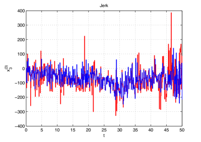
Figure 2: Chassis jerk for MPC with (blue) and without sensitivity update (red)

As expected, the updated control law shows a better performance which can not only be observed from Fig. 2, but also in terms of the closed loop costs: For the chosen industrial road data we obtain an improvement of approximately $8.2\%$ using the sensitivity update (9). Although this seems to be a fairly small improvement, the best possible result obtained by a full reoptimization reveals a reduction of approximately $10.5\%$ of the closed loop costs.

We like to note that due to the presence of constraints it is a priori whether the conditions of Theorem 4.1 hold at each visited point along the closed loop. Such an occurrance can be detected online by checking for violations of constraints or changes in the control structure. Yet, due to the structure of the MPC algorithm, such an event has to be treated if one of the constraints is violated at open loop time instant $k=1$ only which was not the case for our example.

6 Conclusions and Outlook

We considered MPC without stabilizing terminal constraints or Lyapunov type terminal costs in the presence of disturbances. For this setting, we presented stability and performance results for abstract control updates. The required assumptions are shown to be fulfilled if sensitivity updates on the control can be performed.

Future research concerns the analysis of other types of control updates such as realtime iterations which have been considered for MPC with stabilizing terminal constraints and costs. Using the presented result, we hope to obtain a unified stability and performance analysis of MPC in the presence of disturbances and respective control updates. Regarding the halfcar example, the influence of other types of interpolation/extrapolation methods on the MPC performance such as road profiles based on statistical data will be analysed.

This work was partially funded by the German Federal Ministry of Education and Research (BMBF), grant no. 03MS633G.

References

- Alamir [2006] M. Alamir. Stabilization of nonlinear systems using receding-horizon control schemes. Springer, 2006.
- Alamir and Bornard [1995] M. Alamir and G. Bornard. Stability of a truncated infinite constrained receding horizon scheme: the general discrete nonlinear case. Automatica, 31(9):1353–1356, 1995.
- Bock et al. [2007] H.G. Bock, M. Diehl, E.A. Kostina, and J.P. Schlöder. Constrained optimal feedback control of systems governed by large differential algebraic equations. In L. Biegler, O. Ghattas, M. Heikenschloss, D. Keyes, and B. Bloemen Waanders, editors, Real-Time PDE-Constrained Optimization, pages 3–22. SIAM, 2007.
- Camacho and Bordons [2004] E.F. Camacho and C. Bordons. Model Predictive Control. Springer, 2004.
- Chen and Allgöwer [1998] H. Chen and F. Allgöwer. A quasi-infinite horizon nonlinear model predictive control scheme with guaranteed stability. Automatica, 34(10):1205–1218, 1998.
- Diehl et al. [2005] M. Diehl, H.G. Bock, and J.P. Schlöder. A Real–Time Iteration Scheme for Nonlinear Optimization in Optimal Feedback Control. SIAM Journal on Control and Optimization, 43(5):1714–1736, 2005.
- Fiacco [1983] A.V. Fiacco. Introduction to sensitivity and stability analysis in nonlinear programming. Academic Press Inc., 1983.
- Findeisen and Allgöwer [2004] R. Findeisen and F. Allgöwer. Computational Delay in Nonlinear Model Predictive Control. In Proceedings of the International Symposium on Advanced Control of Chemical Processes, 2004.
- Grimm et al. [2005] G. Grimm, M. J. Messina, S. E. Tuna, and A. R. Teel. Model predictive control: for want of a local control Lyapunov function, all is not lost. IEEE Transactions on Automatic Control, 50(5):546–558, 2005.
- Grötschel et al. [2001] M. Grötschel, S.O. Krumke, and J. Rambau. Online Optimization of Large Scale Systems. Springer, 2001.
- Grüne [2009] L. Grüne. Analysis and design of unconstrained nonlinear MPC schemes for finite and infinite dimensional systems. SIAM Journal on Control and Optimization, 48:1206–1228, 2009.
- Grüne and Pannek [2011] L. Grüne and J. Pannek. Nonlinear Model Predictive Control: Theory and Algorithms. Springer, 2011.
- Grüne and Rantzer [2008] L. Grüne and A. Rantzer. On the infinite horizon performance of receding horizon controllers. IEEE Transactions on Automatic Control, 53(9):2100–2111, 2008.
- Jadbabaie and Hauser [2005] A. Jadbabaie and J. Hauser. On the stability of receding horizon control with a general terminal cost. IEEE Transactions on Automatic Control, 50(5):674–678, 2005.
- Jiang and Wang [2001] Z.-P. Jiang and Y. Wang. Input-to-state stability for discrete-time nonlinear systems. Automatica, 37(6):857 – 869, 2001.
- Keerthi and Gilbert [1988] S.S. Keerthi and E.G. Gilbert. Optimal infinite horizon feedback laws for a general class of constrained discrete-time systems: stability and moving horizon approximations. Journal of Optimization Theory and Applications, 57:265–293, 1988.
- Lincoln and Rantzer [2006] B. Lincoln and A. Rantzer. Relaxing dynamic programming. IEEE Transactions on Automatic Control, 51(8):1249–1260, 2006.
- Magni and Scattolini [2007] L. Magni and R. Scattolini. Robustness and robust design of MPC for nonlinear discrete-time systems. In R. Findeisen, F. Allgöwer, and L. T. Biegler, editors, Assessment and future directions of nonlinear model predictive control, volume 358 of Lecture Notes in Control and Information Sciences, pages 239–254. Springer, Berlin, 2007.
- Mayne et al. [2000] D.Q. Mayne, J.B. Rawlings, C.V. Rao, and P.O.M. Scokaert. Constrained model predictive control: Stability and optimality. Automatica, 36(6):789–814, 2000.
- Nevistić and Primbs [1997] V. Nevistić and J. A. Primbs. Receding horizon quadratic optimal control: Performance bounds for a finite horizon strategy. In Proceedings of the European Control Conference, 1997.
- Popp and Schiehlen [2010] K. Popp and W.O. Schiehlen. Ground Vehicle Dynamics. Springer, 2010.
- Primbs and Nevistić [2000] J.A. Primbs and V. Nevistić. Feasibility and stability of constrained finite receding horizon control. Automatica, 36:965–971, 2000.
- Rawlings and Mayne [2009] J. B. Rawlings and D. Q. Mayne. Model Predictive Control: Theory and Design. Nob Hill Publishing, 2009.
- Shamma and Xiong [1997] J.S. Shamma and D. Xiong. Linear nonquadratic optimal control. IEEE Transactions on Automatic Control, 42(6):875–879, 1997. ISSN 0018-9286.
- Speckert et al. [2009] M. Speckert, K. Dreßler, and N. Ruf. Undesired drift of multibody models excited by measured accelerations or forces. Technical report, ITWM Kaiserslautern, 2009.
- Zavala and Biegler [2009] V. M. Zavala and L. T. Biegler. The advanced-step NMPC controller: Optimality, stability and robustness. Automatica, 45(1):86–93, 2009.