Exploring the relation between (sub-)millimeter radiation and $\gamma$-ray emission in blazars with Planck and Fermi

Abstract

The coexistence of Planck and Fermi  satellites in orbit has enabled the exploration of the connection between the (sub-)millimeter and $\gamma$-ray emission in a large sample of blazars. We find that the $\gamma$-ray emission and the (sub-)mm luminosities are correlated over five orders of magnitude, $L_{\gamma}~{}\propto~{}L_{(sub-)mm}$. However, this correlation is not significant at some frequency bands when simultaneous observations are considered. The most significant statistical correlations, on the other hand, arise when observations are quasi-simultaneous within 2 months. Moreover, we find that sources with an approximate spectral turnover in the middle of the mm-wave regime are more likely to be strong $\gamma$-ray emitters. These results suggest a physical relation between the newly injected plasma components in the jet and the high levels of $\gamma$-ray emission.

1 Introduction

Within the three years of its operation, the Fermi satellite has confirmed that the extragalactic $\gamma$-ray sky is dominated by emission from blazars (The Fermi-LAT Collaboration (2011), 2LAC; Ackermann et al., 2011b). A blazar is an unusual type of active galactic nuclei (AGN) in which a relativistic jet points toward Earth, and due to relativistic effects the emission is amplified and variability time scales look shorter. Blazars come in two flavours, with prominent or weak broad-emission lines, and are called Flat Spectrum Radio Quasars (FSRQ) or BL Lac objects (BLLacs), respectively.

However, during the Fermi era it has been shown that not all blazars are strong $\gamma$-ray emitters (e.g. Lister et al., 2011; Giommi et al., 2011), and the likelihood of detection is probably related to faster and brighter jets (e.g. Kovalev et al., 2009; Nieppola et al., 2011), jets pointing closer to our line of sight (Lister et al., 2009), larger apparent jet opening angles (Pushkarev et al., 2009; Ojha et al., 2010), higher variability (e.g. Richards et al., 2011), or the presence of multiple inverse-Compton components (Abdo et al., 2010a; Türler & Björnsson, 2011). In addition, it has been shown that the highest levels of $\gamma$-ray emission are closely related to ejections of superluminal components (e.g. Agudo et al., 2011) and ongoing high-frequency radio flares (León-Tavares et al., 2011). Whether a blazar needs to fulfill all (or a specific combination) of the above conditions in order to radiate in $\gamma$-rays is one of the most important questions that still needs to be answered about the nature of $\gamma$-ray emission in blazars.

The complete diagnostic of what makes a blazar bright at $\gamma$-ray wavelengths requires measurements of the so far poorly explored (sub-)mm spectral bands. Because mm and sub-mm radiation in blazars merely samples the optically thin regime of the synchrotron spectrum, thermal emission (from accretion processes) and radiation from lobes is negligible in these bands (Giommi et al., 2009). Therefore, (sub-)mm measurements can efficiently probe the inner regions of blazar jets and shed light on the region where the bulk of the $\gamma$-ray emission is produced.

In this work we compare Fermi/LAT $\gamma$-ray photon fluxes integrated over three different periods of time with Planck (sub-)mm observations of a sample of blazars. The data are presented in Section 2, and in Section 3 we perform a correlation analysis between intrinsic luminosities in both energy regimes. Section 4 presents an analysis of mm/sub-mm spectral shapes and $\gamma$-ray brightness. Our results are discussed and summarized in Section 5. Throughout this manuscript, we use a $\Lambda$CDM cosmology with values within $1\sigma$ of the WMAP results (Komatsu et al., 2009); in particular, H₀=71 km s^-1 Mpc^-1, $\Omega_{m}=0.27$, and $\Omega_{\Lambda}=0.73$.

2 The data

We build our analysis on the sample of 105 blazars presented in Giommi et al. (2011), who considered three samples of blazars with flux limits in the soft X-rays (count-rates${}_{\ 0.1-2.4\hskip 1.42271ptkeV}>$ 0.3 counts s^-1), hard X-rays (S${}_{\ 15-150\hskip 1.42271ptkeV}>10^{-11}$ erg cm^-2 s^-1), and $\gamma$-ray bands with additional 5 GHz flux density limits. The advantage of using this sample is the availability of $\gamma$-ray flux measurements (quasi-)simultaneous to Planck observations. ESA’s space mission Planck has been surveying the sky at nine frequencies since August 2009 (Planck Collaboration et al., 2011b). Its payload includes two instruments: the Low Frequency Instrument (LFI) operating at 30, 44 and 70 GHz while the High Frequency Instrument (HFI) observes at 100, 143, 217, 353, 545 and 857 GHz. The (sub-)mm flux densities employed in this work are listed in Table 6 of Giommi et al. (2011).

The Fermi/LAT $\gamma$-ray photon fluxes used in this study are based on data in the 100 MeV to 300 GeV energy range and the data processing procedure has been fully described in section 3 of Giommi et al. (2011). For those sources where the Test Statistics (TS) in the whole energy band (0.1 - 300 GeV) delivers a value smaller than 25, an upper limit is given instead. Our gamma -ray data consist of three datasets which we describe below:

• Simultaneous ($<S_{\gamma}>_{sim}$): The $\gamma$-ray photon flux was integrated over the period of time within which the source was observed at all Planck  frequencies. A source in our sample typically sweeps over the Planck focal plane in about 2 weeks. Therefore, $\gamma$-ray photon fluxes integrated during the Planck observation can be considered as simultaneous within one week.

• Quasi-simultaneous ($<S_{\gamma}>_{qua}$): The $\gamma$-ray photon flux densities were obtained by integrating Fermi data over a period covering two months and centered on the Planck observing period, i.e. about one month before and one month after the source was observed by Planck . We consider these $\gamma$-ray data as quasi-simultaneous to the Planck observations on monthly timescales.

• Average ($<S_{\gamma}>_{ave}$): The $\gamma$-ray photon flux was integrated over a long-term period (27 months, from August 2008 to November 2010). We refer to these photon fluxes as average $\gamma$-ray fluxes.

The number of $\gamma$-ray detections (N_det) in each of the above Fermi datasets is as follows: $<N_{det}>_{sim}$ = 26, $<N_{det}>_{qua}$ = 56 and $<N_{det}>_{ave}$ = 81.

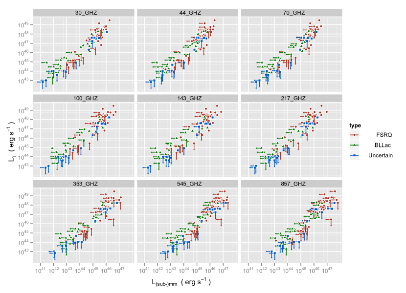
Figure 1: Planck luminosities in (sub-)mm bands versus 27 months average Fermi luminosities. Upper limits in the (sub-)mm and high-energy bands are indicated by left and downward arrows, respectively. Red circles represent FSRQs, green triangles BLLacs, and blue squares sources with uncertain types. The partial correlation parameters for each panel are given in Table 2.

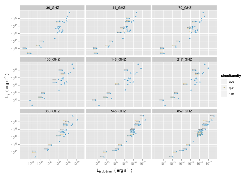
Figure 2: Planck luminosities in (sub-)mm bands versus $\gamma$-ray luminosities using Fermi data averaged over three different periods of time: 2 weeks (sim), 2 months (qua) and 27 months (ave). The partial correlation parameters for each panel are given in Table 3.

3 The (sub-)mm and $\gamma$-ray emission relationship

In order to investigate the physical relation between the $\gamma$-ray and mm/sub-mm emission in blazars, we look for a statistical association between the wavelength regimes on the luminosity-luminosity plane. The reason for performing the correlation analyses using intrinsic luminosities rather than observed fluxes is that the flux-flux correlations will be distorted (and might even vanish) if the coefficient $x$ in the relation $L_{\gamma}\propto L_{\nu}^{x}$ is different from unity (Feigelson & Berg, 1983). On the other hand, if there is no intrinsic luminosity-luminosity correlation then no correlation will appear in the flux-flux plane as shown by Feigelson & Berg (1983). The mm/sub-mm luminosities have been computed according to the following expression,

$$L_{(sub-)mm}=4\pi d_{L}^{2}\frac{\nu S_{\nu}}{(1+z)}~{}\textrm{erg s}^{-1},$$ (1)

where $d_{L}$ is the luminosity distance, $\nu$ corresponds to each of the nine $Planck$ frequencies, and $S_{\nu}$ is the single-epoch flux density taken from Giommi et al. (2011).

The $\gamma$-ray luminosity has been calculated according to

$$L_{\gamma}=4\pi d_{L}^{2}\frac{S_{\gamma}(0.1,300)}{(1+z)^{1-\alpha_{\gamma}}}~{}\textrm{erg s}^{-1},$$ (2)

where $\alpha_{\gamma}=\Gamma-1$, $\Gamma$ being the 27 months average photon spectral index and $S_{\gamma}(0.1,300)$ is the photon energy flux integrated between 0.1 and 300 GeV calculated from the photon flux ($F_{\gamma}$) by using the following expressions,

$$S_{\gamma}(0.1,300)=1.6\times 10^{-4}~{}\frac{\alpha_{\gamma}~{}F_{\gamma}}{1-\alpha_{\gamma}}~{}[3000^{1-\alpha_{\gamma}}-1]~{}\hskip 14.22636pt\alpha_{\gamma}\neq 1$$ (3)

$$S_{\gamma}(0.1,300)=1.28\times 10^{-3}~{}F_{\gamma}\hskip 14.22636pt\alpha_{\gamma}=1$$ (4)

derived from the relations presented in Ghisellini et al. (2009).

3.1 Statistical methods

It is conceivable that the dependence on redshift might induce artificial correlations between the luminosities. For that reason we must apply partial correlation methods to evaluate intrinsic $L_{\gamma}-L_{\nu}$ correlations. Because of the presence of upper limits in some of the $\gamma$-ray flux and (sub-)mm flux density measurements in our sample, survival analysis techniques are needed to properly quantify the correlation coefficient between these two emission bands. Therefore we have applied the Kendall’s tau partial correlation for censored data (Akritas & Siebert, 1996) to estimate whether there is an intrinsic correlation between luminosities once the influence of the upper limits has been taken into account and the common dependence on redshift has been removed.

The FORTRAN code cens_tau implements the methods presented in Akritas & Siebert (1996) providing a measure of the correlation between the two luminosities while excluding the effects of the redshift ($\tau_{LLz}$). The probability that non-correlation exists between luminosities (P_τ) can be gleaned from the output of the code as well. We consider a partial correlation significant if the probability of non-correlation is less than 5% (P${}_{\tau}<$ 0.05).

The slope of the correlations between (sub-)mm and $\gamma$-ray bands has been computed by the Akritas-Theil-Sen nonparametric regression method implemented in the routine cenken of the R package NADA. This method is best suited to our purposes owing the presence of upper limits in both variables.

3.2 Significance test using the method of surrogate data

To ensure that an intrinsic luminosity-luminosity correlation has not been drawn by chance we employed surrogate data (uncorrelated (sub-)mm and $\gamma$-rays luminosity pairs) to quantify whether the correlation coefficient obtained by applying the censored partial correlation test can or cannot be reproduced by mere coincidence. Based on the surrogate method described in detail in Ackermann et al. (2011a), we constructed surrogate luminosity data sets by following the next procedure:

1. We start with a sample of $m$ sources with a firm measurement of their redshift. The (sub-)mm and $\gamma$-ray luminosities are thus estimated by using expressions (1) and (2), respectively. Then, we run the censored partial correlation test to quantify the observed correlation strength ($\tau_{0}$).

2. The sample is split in $n$ redshift bins, each bin should contain at least 10 sources. This criterion follows the arguments described in section 4 of Ackermann et al. (2011a).

3. In each bin we randomly shuffle the redshift and both the (sub-)mm and $\gamma-$ray luminosities. The censored status of the luminosities at each band – either detected or upper limit – sticks to the original luminosity value.

4. Using the surrogates from each bin, we build an uncorrelated data set of $m$ pairs of luminosities with randomly assigned redshifts. Then we run the censored partial correlation test to estimate the correlation coefficient $\tau_{i}$ and the probability that the surrogate data set is non-correlated (P${}_{i})$.

5. We repeat the steps 3 and 4 a large number of times (N_trials) and build the distribution of correlation coefficients for these surrogate uncorrelated luminosity pairs.

We use the distribution of random correlation coefficients built on N${}_{trials}=1000$ to compute the probability of obtaining a significant correlation (P${}_{i}<$ 0.05) with a coefficient larger or equal (in terms of absolute value) than the observed one. Then, the significance of the observed censored partial correlation (P_surrogate) is estimated by computing the ratio N${}_{hits}/$N_trials, where N_hits is he number of times that we registered a significant correlation with $|\tau_{i}|\geq\tau_{0}$.

An observed censored partial correlation is considered real only if the probability of getting the same (or a larger) correlation coefficient is less than 5% (P${}_{surrogate}<0.05$). This criterion will ensure us that observing a significant (sub-)mm ad $\gamma$-ray luminosity-luminosity partial correlation with a coefficient $\tau_{0}$ is not likely to occur by chance.

3.3 The L_γ - L_(sub-)mm correlation

We investigate the luminosity-luminosity correlation between the (sub-)mm emission and $\gamma$-ray fluxes in the sample of blazars presented in Giommi et al. (2011). We only consider sources with firm measurements of their redshift and $\gamma$-ray photon flux – either detection or upper limit– leaving us with a total of 98 sources. The luminosities at the (sub-)mm and $\gamma$-ray regimes were computed according to expression 1 and 2, respectively. In equation (2), $S_{\gamma}(0.1,300)$ is the photon energy flux integrated over 27 months ($<S_{ave}>$). For those cases where non-detection of the sources was possible, we estimate an upper limit of the luminosity assuming the average photon spectral index for our sample, $<\Gamma>=1.38$. All luminosities are listed in Table 1.

Figure 1 shows the luminosity-luminosity relation between all (sub-)mm frequency bands and average values of $\gamma$-ray emission obtained by integrating Fermi data over 27 months. In order to examine the possible dependence of the correlation on blazar type, the various blazar types are symbol coded as shown in the legend of Figure 1. FSRQs populate the upper right part of the luminosity-luminosity plane, whereas BLLacs and sources with uncertain type continue the trend toward lower luminosities. It should be noticed that some of the sources classified as “uncertain type” are actually known radio galaxies, however, for sake of consistency we keep the nomenclature as stated in Tables 1 to 3 of Giommi et al. (2011)

The correlation parameters and their significances for each of the panels of Figure 1 are summarized in Table 2. The statistical methods described in the above subsections reveal that mm/sub-mm luminosities are positively correlated with $\gamma-$ray luminosities over five orders of magnitude when all source types are considered. However, differences arise when we compute partial correlations for FSRQs and BLLacs, separately. The correlations between (sub-)mm and $\gamma$-ray emission bands are significant and real when FSRQs are considered only. However, the surrogate test method does not provide evidence that correlations for BLLacs are significant.

The slope of the relation between (sub-)mm and $\gamma$-ray luminosities has been computed with the Akritas-Theil-Sen nonparametric regression method and the fitted values are also listed in Table 1. For all 98 sources considered in our study, the (sub-)mm - $\gamma$-ray luminosity relation can be well approximated as $L_{\gamma}\sim L_{\nu}^{x}$, where $<x_{All}>=1.27\pm 0.02$. The slope fitted for BLLacs ($<x_{BLLac}>=1.13\pm 0.03$) is somewhat shallower than the slope computed for FSRQ ($<x_{FSRQ}>=1.40\pm 0.03$). While the different photon spectral index between FSRQs and BLLacs (Ghisellini et al., 2009) may play some role in the difference between fitted slopes, the lack of correlation for BLLacs might indicate that different radiation mechanisms are behind the $\gamma$-ray emission. As we discuss in section 4, clean and well characterized samples of BLLacs are needed to get further insight into the physical conditions that make the difference between FSRQs and BLLacs.

The low detection rate at the highest Planck frequencies can be a combination of the high flux density detection limit at these frequencies – see Table 3 in Planck Collaboration et al. (2011c), and the fact that blazars in general become brighter at submm frequencies only during flaring states (e.g Marscher & Gear, 1985; Raiteri et al., 2011). Therefore, due to the relatively low number of sources detected at 545 and 857 GHz the correlation and best-fitted line parameters for these frequency bands shown in Table 2 and 3 should be taken with caution.

3.4 Dependence of the L_γ - L_(sub-)mm correlation on simultaneity

We find that in our sample of blazars the $\gamma$-ray emission averaged over large periods of time (i.e. 27 months) is significantly correlated to the (sub-)mm radiation. This result suggests a coupling of the emitting regions, however, to get a physical insight about this relation we next need to investigate whether the correlation between (sub-)mm and $\gamma$-ray emission bands shows a trend for strengthening with simultaneity. We emphasize again that our Fermi data set contains information about the $\gamma$-ray emission averaged over three different periods of time, allowing us to assess the intrinsic correlation between (sub-)mm radiation and simultaneous, quasi-simultaneous and averaged $\gamma$-ray emission.

To investigate the dependence of the $L_{\gamma}$ - $L_{(sub-)mm}$ correlation on simultaneity of the data, the levels of censoring at $\gamma$-rays must be controlled and therefore we only consider sources that were detected by Fermi at each of the three averaging periods. Hereafter we refer to this subsample as the Fermi-detected sample which comprises 24 sources. Most of them are classified as FSRQ type and based on their simultaneous SEDs all of them have been classified as low-synchrotron peaked (LSP) in Giommi et al. (2011).

Figure 2 shows the luminosity-luminosity relation for all (sub-)mm frequency bands and $\gamma$-ray emission integrated over three different periods of time. The simultaneity of the $\gamma$-ray emission to the Planck measurements is symbol coded as shown in the legend at the right center of the plot. Table 3 reports the partial correlation parameters and associated probabilities for the three $\gamma$-ray data sets.

As can be seen from Table 3, it is noticeable that the strongest correlations arise when Fermi  measurements have been integrated over long periods of time (2 and 27 months), whereas the weakest and less significant correlations are always obtained when simultaneous observations are involved. The remarkably stronger correlation with the $\gamma$-ray photon fluxes integrated over 27 months is likely an artificial effect due to averaging the $\gamma$-ray photon fluxes over a very long period of time. This reduces the dynamical range of $\gamma$-ray photon flux observed (Muecke et al., 1997), which in turn reduces the scatter of the $L_{\gamma}$-$L_{\nu}$ relation and improves the correlation strength. Given the evidence that the strongest $\gamma$-ray flares tend to have a short duration time, with a typical timescale of a month (see Abdo et al., 2010b), one might argue that by averaging $\gamma$-ray data over two months we may be averaging flares, which would reduce the dynamical range of quasi-simultaneous $\gamma$-ray luminosities, and therefore stronger correlations may be induced. However, it is not likely that all sources considered in our study were flaring during the weeks that $Planck$ observed them. This leads us to believe that the the most significant correlations in our study arise when using the $\gamma$-ray photon fluxes averaged over 2 months.

4 Shape of the synchrotron spectra and $\gamma$-ray brightness

In this section we explore emerging trends between (sub-)mm spectral shape and $\gamma$-ray brightness with the aim to find out whether the (sub-)mm spectrum shape can be considered as a new piece to the puzzle of what makes a blazar shine at $\gamma$-rays. The radio to sub-mm spectra can be well approximated by two power laws (e.g. Gear et al., 1994; Planck Collaboration et al., 2011a), however the point where both power laws connect has always been assumed rather arbitrarily based on the spectral coverage of the data sets involved. This in turn might introduce some biases to the spectral indices fitted to parametrize the spectral shapes.

Hence, in this work we use a different approach by fitting the Planck observations from 30 to 857 GHz with a broken power law model where the fiducial point where the intersection of the power laws occurs is considered as a free parameter along the fit. The expression of the broken power law used to model the (sub-)mm spectral range is given by,

$$S(\nu)\propto\begin{cases}\nu^{\alpha_{mm}}&\mbox{for}~{}\nu\leq\nu_{break}\\ \nu_{break}^{(\alpha_{mm}-\alpha_{submm})}\nu^{\alpha_{submm}}&\mbox{for }\nu>\nu_{break},\end{cases}$$ (5)

where $\alpha_{mm}$ and $\alpha_{submm}$ are the spectral indices for the mm and sub-mm part of the spectrum, respectively, and the two power laws are connected at the break frequency $\nu_{break}$.

To perform the analysis of spectral shapes and $\gamma$-ray brightness, we select only those sources from Giommi et al. (2011) that have been detected in at least five Planck frequency bands, this with the aim to produce a reliable modeling of the spectra. The 47 sources selected based on the criterion mentioned above, along with the best-fit model parameters, are listed in Table 4.

The new (sub-)mm observations provided by the Planck satellite and their modeling with a broken power law function allow us to typecast the (sub-)mm spectral shapes in our sample. Figure 3 shows all four spectral shapes that could possibly be found in our sample. Next we describe their characteristics and possible interpretation in terms of multicomponent synchrotron spectra:

1. Steep $\alpha_{mm}$ - Steep $\alpha_{submm}$: (sub-)mm emission decreases monotonically with frequency. This straight spectral shape from mm to sub-mm regimes is dominated by the underlying emission from a component with a synchrotron turnover frequency located at cm wavelengths. Quiescent activity levels (i.e. no new young synchrotron components) is expected for sources featuring this spectral type.

2. Steep $\alpha_{mm}$ - Flat/rising $\alpha_{submm}$: mm spectrum is dominated by the emission from an aged component that becomes self absorbed at the cm regime, as in $(A)$. Despite that, a flat/rising $\alpha_{submm}$ spectrum betrays the presence of a new component in an early development stage, located well within the radio core region. Then a new flare connected to the ejection of a new VLBI component is likely to occur before the sub-mm spectrum steepens. It is possible that a rising $\alpha_{submm}$ could also be related to the presence of a dust component, however, a more detailed dissection of the spectra is needed to assess its presence.

3. Flat $\alpha_{mm}$ - Steep $\alpha_{submm}$: An overall flatness of the mm spectrum can be explained by a succession of several components in the jet as stated in the so-called “cosmic conspiracy” (Cotton et al., 1980). Nevertheless, the steepening of the submm spectra is consistent with synchrotron emission from a single component which becomes self absorbed somewhere in the middle of the mm wavelength regime.

4. Rising $\alpha_{mm}$ - Steep $\alpha_{submm}$: In the absence of adjacent strong spectral components at lower or higher frequencies, a new component recently ejected from the radio core, with a self absorbed spectrum peaking in the mm regime, dominates the overall shape of the radio spectrum.

The (sub-)mm spectra of the selected blazars were classified into the above spectral categories based on the relative difference between spectral indices $\Delta\alpha=\frac{\alpha_{submm}-\alpha_{mm}}{\alpha_{mm}}$. The spectral classification for the 47 sources selected is reported in Table 4 and is defined by the following conditions:

• A : $\alpha_{mm},\alpha_{submm}<0$ and $|\Delta\alpha|<0.5$; relative difference between indices is less than 50%,

• B: $\alpha_{mm}<0$ and $\alpha_{submm}\geq 0$,

• C : $\alpha_{mm},\alpha_{submm}<0$ and $|\Delta\alpha|>0.5$; relative difference between indices is greater than 50%,

• D: $\alpha_{mm}>0$ and $\alpha_{submm}<0$,

The classification scheme described above is sketched in Figure 3, which attempts to compare the (sub-)mm spectral shapes of blazars at different stages of the synchrotron components evolution. Based on successive approximations, we further group the four categories into two main spectral classes: (i) A-B includes sources previously classified as A or B , these represent the quiescent and the very initial stages of an ejected component, respectively. (ii) The spectral type C-D is conformed by sources whose spectral shapes are categorized as type C or D, these specific spectral features indicate the presence of a freshly ejected synchrotron component where the spectral turnover is somewhere in the middle of the mm wave regime.

Based on the latter spectral type classification, we may classify our sample into 23 sources of category A-B and 24 sources falling into the category of C-D. Figures 4 and 5 show the (sub-)mm spectra for both spectral types and overplotted are the best-fits to the (sub-)mm spectra using the broken power law model.

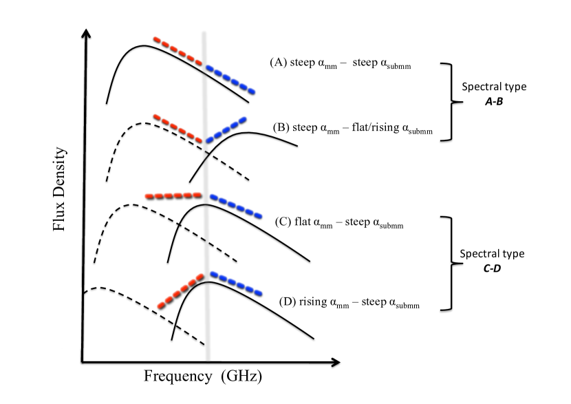
Figure 3: An illustration of all synchrotron spectral shapes we could possibly find in our sample, see text for detailed description. The overall spectrum has been approximated by a broken power law with spectral indices $\alpha_{mm}$ (red) and $\alpha_{sub-mm}$ (blue), respectively. The break frequency ($\nu_{break}$) is indicated by the grey thick vertical line. Aged synchrotron components are represented by dashed lines

Due to the fact that $L_{\gamma}-L_{\nu}$ are best correlated when using quasi-simultaneous $\gamma$-ray fluxes ($<S_{\gamma}>_{qua}$), we proceeded to find out if there is a pattern in the spectral shapes that relates to the levels of quasi-simultaneous $\gamma$-ray emission. Figure 6 shows the quasi-simultaneous $\gamma$-ray flux distributions as boxplots. The levels of $\gamma$-ray emission for sources with (sub-)mm spectra belonging to the spectral classes A and B (spectral type A-B) are displayed in the left boxplot of Figure 6 while sources with spectra of the type C and D (spectral type C-D) are shown in the boxplot to the right. Upper limits and detections are symbol coded as denoted in the legend of Figure 6.

At first glance, it seems that sources of the spectral type C-D are brighter at $\gamma$-rays than sources of the spectral type A-B. This can be gleaned from the size of the boxplots and the locations of the medians represented by the thick line at the middle of the boxes displayed in Figure 6. Differences in the distribution of quasi-simultaneous $\gamma$-ray photon fluxes for sources with different (sub-)mm spectral types were statistically investigated. Because of the presence of upper limits to the $\gamma$-ray photon fluxes we apply the univariate two sample tests implemented in the ASURV package (Isobe et al., 1986; Lavalley et al., 1992) to the $\gamma$-rays photon flux distributions displayed in Figure 6. We further consider that two populations are significantly different if the probability that the differences between populations arise by chance is P $\leq 0.05$.

All five two-sample tests implemented in ASURV (Gehan’s generalized Wilcoxon test – permutation variance, Gehan’s generalized Wilcoxon test – hypergeometric variance, logrank test, Peto-Peto generalized Wilcoxon test and Peto-Prentice generalized Wilcoxon test) converge to the same result: the levels of $\gamma$-ray emission of spectral types A-B and C-D are significantly different and the probability that such difference arises by chance is less than 4%. The statistical tests show that the shapes and medians of the distributions of $\gamma$-rays for spectral types A-B and C-D are significantly different, where the levels of $\gamma$-ray emission for sources belonging to the type C-D are significantly higher than for those classified as A-B.

We note that other classification schemes for blazars have already been proposed based on the variability of the radio continuum spectra from cm to mm wavelengths (Angelakis et al., 2011). However, the classification scheme proposed in this work – based on successive approximations of the synchrotron components evolution – for the fist time permits to use the (sub-)mm spectral shapes as flags for high levels of $\gamma$-ray emission.

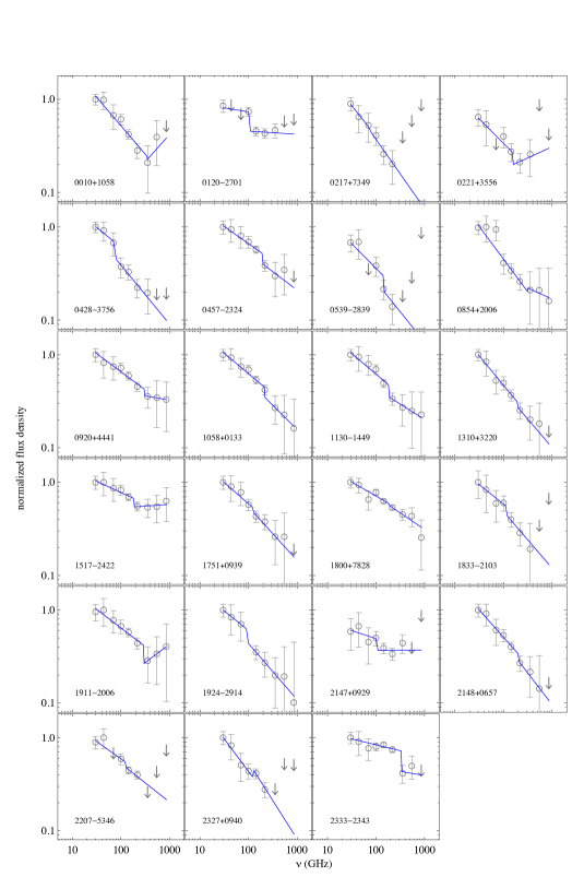
Figure 4: The (sub-)mm spectra for 23 sources classified within the spectral type A-B. See Figure 3 for a visual description of the types.

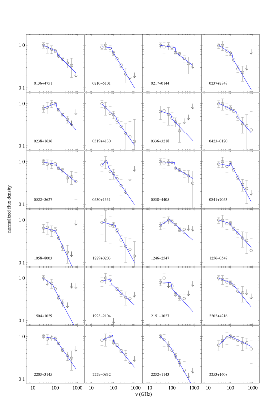
Figure 5: The (sub-)mm spectra for 24 sources classified within the spectral type C-D. See Figure 3 for a visual description of each spectral type.

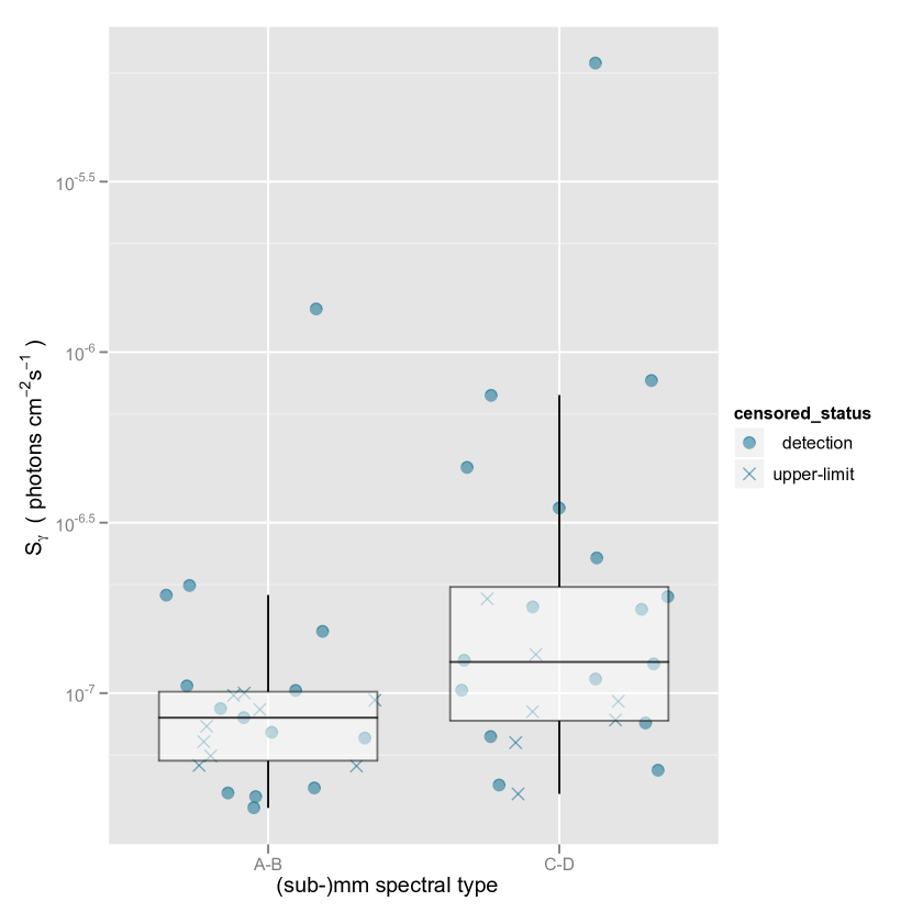
Figure 6: The distribution of of $\gamma$-ray emission levels for sources with spectral types A-B (left) and C-D (right) are shown in boxplots, where the thick line at the middle of the box represents the median. The boxes comprise 75% of the distributions. The levels of $\gamma$-ray emission for sources belonging to the type C-D are significantly higher than for those classified as A-B

5 Discussion and summary

While various studies during the Fermi-era have found evidence for a correlation between radio and $\gamma$-rays (e.g. Kovalev et al., 2009; Ackermann et al., 2011a; Ghirlanda et al., 2011; Nieppola et al., 2011), our work addresses for the first time this connection at (sub-)mm wavelengths. We have found a significant correlation between (sub-)mm and $\gamma$-ray luminosities over five orders of magnitude. Since we have made use of partial-correlation, surrogate data methods and survival analysis techniques we are confident that the correlation $L_{\gamma}\propto L_{\nu}$ is not an artifact of the detection limits, chance or due to the common dependence on redshift. This result is consistent with previous studies (e.g. Ackermann et al., 2011a; Ghirlanda et al., 2011; Nieppola et al., 2011; Arshakian et al., 2012), albeit using high frequency radio observations. Giommi et al. (2011) do not report evidence of a significant correlation between 143 GHz and $\gamma$-ray fluxes in some of the sub-samples considered. This apparently contradiction with our findings is not likely to be influenced by sources without redshift not considered in this study. Instead, such difference may be attributable to the fact that correlations in the flux-flux plane can vanish if the slope of the luminosity-luminosity correlation is different from unity (see discussion in Section 3) as it turns out to be the case for the $L_{\gamma}\propto L_{(sub-)mm}$ relation (see Table 2).

The positive correlation between luminosities is still robust and becomes even stronger when only FSRQs are considered, however, the correlation vanishes for BLLacs as a group. In addition, the slope of the fitted $L_{\gamma}\propto L_{\nu}^{x}$ relation is shallower for BLLacs. The different gamma-radio behavior between blazar types has been found in previous studies using 37 GHz data (León-Tavares et al., 2011; Nieppola et al., 2011). On the other hand, previous studies at low frequencies (Ghirlanda et al., 2011; Ackermann et al., 2011a) find that the radio-gamma correlation is significant for both FSRQs and BLLacs, separately. This apparent discrepancy might be related to the fact that submm spectral indices of FSRQs and BLLacs have been found to be significantly different (Gear et al., 1994). The latter result was interpreted as an intrinsic difference in the underlying jets of BLLacs and FSRQ. Unfortunately due to the low number of BLLacs in the sample analyzed in section 4 – see Table 4, we could not explore this difference with the new (sub-)mm observation.

Nevertheless, before speculating into real physical differences between FSRQs and BLLacs, we would like to rise a word of caution regarding the correlation results solely for the BLLac population. Giommi et al. (2012) have drawn attention to the fact that some sources classified as BLLacs might have been misclassified with FSRQ. This issue can be a direct consequence of the rather artificial criterion that draws the line between FSRQs and BLLacs – rest frame equivalent width (EW) less than $5\AA$ – introduced twenty years ago (Stickel et al., 1991). It is plausible that a particular source was originally classified as BLLac at the time when its non-thermal optical continuum was prominent and high enough to swamp any broad emission line in the optical spectral range, as recently shown in Padovani et al. (2012). However, after some time the same source could have been classified as FSRQ when the optical continuum emission weakened, allowing the exhibition of broad emission lines. To overcome this misclassification problem we should adopt a new blazar taxonomical criterion to classify sources with intrinsically prominent and weak broad-line regions as recently proposed in Ghisellini et al. (2011) and Giommi et al. (2012). Therefore a compilation of a large sample of true BLLacs whose parent population includes low-excitation radio galaxies (LERG) displaying FR-I morphologies, as proposed in Giommi et al. (2012), is highly desirable to draw robust conclusions on the (sub-)mm and $\gamma$-ray connection in BLLacs.

We now turn to the dependence of the $L_{\gamma}\propto L_{\nu}$ relation on simultaneity. Although the strongest correlation parameters are achieved when using $Fermi$ $\gamma$-ray photon fluxes averaged over 27 months, we believe that such tight correlations are a consequence of averaging the $\gamma$-ray photon fluxes over a very long period of time. This reduces the scatter of the $L_{\gamma}$-$L_{\nu}$ relation while the detection of faint $\gamma$-ray sources increases the $\gamma$-ray luminosity dynamical range, hence the correlation strengths are artificially enhanced. Furthermore, the $L_{\gamma}\propto L_{\nu}$ relation becomes weak if $\gamma$-ray and (sub-)mm data are obtained simultaneously. On the other hand, including quasi-simultaneous observations within monthly timescales produces a more significant correlation. This might suggest an intrinsic delay between the emission in both wavebands, however, with the data currently available we cannot disentangle whether the (sub-)mm emission leads the production of $\gamma$-rays or vice versa. There is, however, recent evidence of delays on monthly scales between mm and $\gamma$-ray emission bands, the onset of a mm-flare occurring about 2 months before the maximum of the $\gamma$-ray emission is reached (León-Tavares et al., 2011).

Perhaps the most remarkable result we find is that brighter $\gamma$-ray sources tend to show a specific shape in their radio spectra, i.e. flat/rising mm and falling sub-mm spectral indices (spectral type C-D), see Figure 3 for the classification scheme proposed in this work. This spectral shape is consistent with a single synchrotron component becoming self absorbed in the middle of the millimeter wavelength regime that must be responsible for the last spectral turnover. Despite the fact that we have not attempted to properly dissect the (sub-)mm spectra into single synchrotron components, turnover frequencies for sources of the spectral type C-D can be roughly constrained to $\nu_{m}>$ 30 GHz.

Our finding that $\gamma$-ray emission is enhanced in sources of the spectral type C-D – featuring an approximate spectral turnover at the middle of the mm wavelength regime – suggests an important role of the plasma jet disturbances, responsible for shaping the (sub-)mm spectra, in producing the $\gamma$-ray emission. Since $B\propto\nu_{m}^{5}$ (Lobanov, 1998) sources of the spectral type C-D ($\nu_{m}>30$ GHz) are expected to harbor strong magnetic fields in their cores leading to polarized emission. This argument finds support in recent observational results by Linford et al. (2012), where it was found that strong core polarization is related to intense $\gamma$-ray emission.

The existence of large magnetic fields may reflect in either large electron densities in the emitting region (in this case spectra must be dominated by emission from the core) or the presence of growing shocks emerging from the radio core region. To disentangle the nature of the emission shown in the snapshot (sub-)mm spectra of Figures 4 and 5, multifrequency VLBI monitoring is highly desirable to properly dissect the spectra into individual components (e.g. Lobanov & Zensus, 1999; Savolainen et al., 2008) and to identify the contribution of the core and the emerging shocks to the overall radio spectrum. In addition, upcoming Planck data releases will allow us to build multi-epoch (sub-)mm spectra. Then, by studying the evolution of the spectral shapes, we can get an insight into the changes of the physical properties of the jet (e.g., density, magnetic field, Doppler factor), and those must serve as input to theoretical models aiming to reproduce the levels of $\gamma$-ray emission observed.

In summary, we have used a joint sample of soft X-ray, hard X-ray and $\gamma$-ray selected blazars to explore for the first time the relationship between (sub-)mm emission from 30 to 857 GHz and $\gamma$-ray photon fluxes integrated over three different periods of time: when a source was in the Planck field of view, one month before and after the source was observed by Planck, and over 27 months. Our findings can be listed as follows:

• We have found a significant correlation between $\gamma$-ray and (sub-)mm luminosities which holds over five orders of magnitude. Moreover, using a sample of bright $\gamma$-ray sources detected by Fermi on each of the averaging periods mentioned above, we find – based on our statistical analysis and bearing in mind that $\gamma$-ray photon fluxes averaged over long periods of time (i.e. 27 months) enhance artificially the correlation strength – that quasi-simultaneous observations (within 2 months) showed the most significant statistical correlations.

• Sources with high levels of $\gamma$-ray emission show a characteristic signature in their radio spectra: flat/rising mm and steep sub-mm spectral indices (spectral type C-D in Figure 3). This spectral shape can be associated with a single synchrotron component which becomes self absorbed in the middle of the mm wavelength regime. Such high spectral turnover frequencies reveal the presence of emerging disturbances in the jet which are likely to be responsible for the high levels of $\gamma$-ray emission.

Table 1: Luminosities

J2000_Name	Alias	RA	DEC	$z$	log L30	log L44	log L70	log L100	log L143	log L217	log L353	log L545	log L857	$<logL_{\gamma}>_{sim}$	$<logL_{\gamma}>_{qua}$	$<logL_{\gamma}>_{ave}$
0010+1058	IIIZW2	2.629	10.975	0.089	43.14	43.30	43.33	43.45	43.44	43.45	43.53	43.99	$<$ 44.37	$<$ 45.34	$<$ 44.94	$<$ 44.42
0017+8135	S50014+813	4.285	81.586	3.387	$<$ 45.59	$<$ 45.90	$<$ 46.04	$<$ 45.92	$<$ 45.84	$<$ 46.00	$<$ 47.09	$<$ 47.37	$<$ 47.82	$<$ 48.98	$<$ 48.75	$<$ 48.25
0048+3157	Mkn348	12.196	31.957	0.015	$<$ 41.00	$<$ 41.35	$<$ 41.38	$<$ 41.22	$<$ 41.18	41.40	$<$ 41.94	$<$ 42.44	$<$ 42.56	$<$ 43.46	$<$ 43.11	$<$ 41.91
0120-2701	1Jy0118-272	20.132	-27.023	0.557	44.25	$<$ 44.49	$<$ 44.60	44.71	44.66	44.82	45.06	$<$ 45.41	$<$ 45.63	$<$ 47.18	46.86	46.77
0136+4751	S40133+47	24.244	47.858	0.859	45.40	45.51	45.67	45.80	45.82	45.93	46.06	46.19	$<$ 46.23	$<$ 47.63	47.43	47.51
0204-1701	PKS0202-17	31.240	-17.022	1.740	45.32	$<$ 45.48	45.59	45.65	45.61	45.48	$<$ 46.14	$<$ 46.64	$<$ 47.05	$<$ 48.30	$<$ 47.94	47.80
0210-5101	PKS0208-512	32.693	-51.017	1.003	45.21	45.42	45.56	45.59	45.62	45.65	45.65	$<$ 45.85	$<$ 46.07	$<$ 47.65	47.30	47.51
0214+5144	GB6J0214+5145	33.575	51.748	0.049	$<$ 41.93	$<$ 42.29	$<$ 42.48	$<$ 42.27	$<$ 42.11	$<$ 42.34	$<$ 42.98	$<$ 43.47	$<$ 43.89	$\cdots$	$<$ 44.17	$<$ 43.30
0217+0144	PKS0215+015	34.454	1.747	1.715	45.65	45.78	46.00	46.13	46.15	46.30	46.41	46.48	$<$ 46.69	$<$ 48.63	48.38	48.17
0217+7349	1Jy0212+735	34.378	73.826	2.367	46.06	46.08	46.19	46.24	46.19	46.27	$<$ 46.83	$<$ 47.19	$<$ 47.56	$\cdots$	$<$ 48.40	48.23
0221+3556	1Jy0218+357	35.273	35.937	0.944	44.90	44.99	$<$ 45.04	45.22	45.21	45.28	45.57	$<$ 46.35	$<$ 46.23	$<$ 48.02	47.37	47.60
0237+2848	4C28.07	39.468	28.802	1.213	45.38	45.55	45.62	45.73	45.72	45.69	45.82	$<$ 46.19	$<$ 46.75	$<$ 48.40	48.02	47.95
0238+1636	PKS0235+164	39.662	16.616	0.940	44.90	45.09	45.38	45.53	45.54	45.62	45.71	$<$ 45.87	$<$ 46.33	$<$ 48.06	$<$ 47.54	47.99
0319+4130	NGC1275	49.950	41.512	0.018	42.54	42.61	42.68	42.80	42.83	42.87	42.90	43.01	43.10	$\cdots$	44.38	44.19
0336+3218	NRAO140	54.125	32.308	1.259	45.41	45.59	45.71	45.78	45.85	45.82	$<$ 46.32	$<$ 46.60	$<$ 47.05	$<$ 48.04	$<$ 48.09	47.64
0423-0120	PKS0420-01	65.816	-1.342	0.916	45.70	45.87	45.97	46.12	46.21	46.25	46.30	46.44	46.54	$<$ 48.03	47.72	47.63
0428-3756	PKS0426-380	67.168	-37.939	1.030	45.39	45.52	45.59	45.48	45.58	45.60	45.75	$<$ 45.99	$<$ 46.19	$<$ 47.70	47.77	48.28
0433+0521	3C120	68.296	5.354	0.033	42.26	42.33	42.35	42.59	42.66	42.63	$<$ 42.66	$<$ 43.14	$<$ 43.60	$<$ 44.29	$<$ 43.93	$<$ 43.62
0457-2324	PKS0454-234	74.263	-23.414	1.003	45.22	45.36	45.49	45.58	45.65	45.66	45.76	46.02	$<$ 46.21	48.12	47.95	48.18
0522-3627	PKS0521-36	80.741	-36.458	0.055	43.03	43.13	43.33	43.50	43.55	43.68	43.71	43.93	44.01	$<$ 44.47	44.39	44.68
0530+1331	PKS0528+134	82.735	13.532	2.070	45.76	46.01	45.98	46.08	46.12	46.14	$<$ 46.28	$<$ 46.77	$<$ 47.19	$<$ 48.93	$<$ 48.55	48.47
0538-4405	PKS0537-441	84.710	-44.086	0.892	45.66	45.80	46.02	46.16	46.19	46.33	46.45	46.58	46.61	48.45	48.43	48.21
0539-2839	1Jy0537-286	84.976	-28.665	3.104	45.87	46.04	$<$ 46.02	46.15	46.05	46.04	$<$ 46.43	$<$ 46.82	$<$ 47.49	$<$ 49.07	$<$ 48.99	48.81
0550-3216	PKS0548-322	87.669	-32.272	0.069	$<$ 42.35	$<$ 42.68	$<$ 42.78	$<$ 42.59	$<$ 42.46	$<$ 42.68	$<$ 43.25	$<$ 43.52	$<$ 43.90	$<$ 45.87	$<$ 45.23	43.84
0623-6436	IRAS-L06229-643	95.782	-64.606	0.129	43.00	43.37	43.25	43.25	$<$ 43.06	$<$ 43.19	$<$ 44.28	$<$ 44.56	$<$ 45.01	$<$ 44.93	$<$ 45.12	$<$ 44.84
0738+1742	PKS0735+17	114.530	17.705	0.424	44.08	$<$ 44.33	$<$ 44.44	$<$ 44.15	$<$ 44.13	$<$ 44.27	$<$ 45.36	$<$ 45.63	$<$ 46.09	$<$ 46.97	46.54	46.59
0746+2549	B2.20743+25	116.608	25.817	2.979	$<$ 45.63	$<$ 45.97	$<$ 46.05	$<$ 45.79	$<$ 45.77	$<$ 45.91	$<$ 47.00	$<$ 47.28	$<$ 47.73	$<$ 49.49	$<$ 48.34	48.56
0818+4222	S40814+425	124.567	42.379	0.530	44.59	44.64	$<$ 44.64	$<$ 44.35	$<$ 44.33	$<$ 44.47	$<$ 45.56	$<$ 45.84	$<$ 46.29	$<$ 47.25	46.69	46.94
0824+5552	OJ535	126.197	55.878	1.417	$<$ 45.01	$<$ 45.39	$<$ 45.47	$<$ 45.25	45.35	$<$ 45.41	$<$ 45.95	$<$ 46.40	$<$ 46.59	$<$ 48.06	$<$ 47.85	47.57
0841+7053	4C71.07	130.351	70.895	2.218	46.01	46.23	46.32	46.56	46.55	46.56	46.60	46.69	$<$ 46.85	$<$ 48.47	$<$ 48.60	48.49
0854+2006	PKS0851+202	133.703	20.108	0.306	44.76	44.94	45.11	44.91	44.98	45.04	45.16	45.35	45.43	$<$ 46.20	45.98	46.16
0920+4441	S40917+44	140.243	44.698	2.190	45.95	46.03	46.19	46.33	46.40	46.47	46.57	46.75	46.92	48.88	48.69	48.76
0923-2135	PKS0921-213	140.912	-21.596	0.053	$<$ 41.99	$<$ 42.39	$<$ 42.41	$<$ 42.36	42.42	42.54	42.96	$<$ 43.48	$<$ 43.66	$\cdots$	$<$ 44.25	$<$ 44.00
0957+5522	4C55.17	149.409	55.383	0.896	44.89	$<$ 44.99	$<$ 45.06	45.03	45.07	45.09	$<$ 45.45	$<$ 46.08	$<$ 46.19	47.75	47.74	47.66
1015+4926	1H1013+498	153.767	49.433	0.212	$<$ 43.35	$<$ 43.69	$<$ 43.78	$<$ 43.50	$<$ 43.46	$<$ 43.59	$<$ 44.25	$<$ 44.71	$<$ 44.90	45.90	45.91	45.99
1058+0133	4C01.28	164.623	1.566	0.888	45.58	45.71	45.82	45.94	45.98	46.06	46.08	46.19	46.24	$<$ 47.69	47.39	47.51
1058+5628	1RXSJ105837.5+562816	164.657	56.470	0.143	$<$ 42.96	$<$ 43.32	$<$ 43.40	$<$ 43.24	$<$ 43.11	$<$ 43.21	$<$ 43.90	$<$ 44.36	$<$ 44.54	45.67	45.56	45.38
1058-8003	PKS1057-79	164.680	-80.065	0.581	44.73	44.91	45.04	45.21	45.18	45.14	45.23	$<$ 45.44	$<$ 46.37	$<$ 46.90	46.68	46.68
1104+3812	Mkn421	166.114	38.209	0.030	$<$ 41.48	$<$ 41.95	$<$ 42.04	41.89	$<$ 41.83	$<$ 41.99	$<$ 42.55	$<$ 43.04	$<$ 43.46	44.95	44.98	44.92
1127-1857	PKS1124-186	171.768	-18.955	1.048	45.15	45.25	45.24	45.53	45.60	45.70	45.88	$<$ 46.01	$<$ 46.38	47.82	47.86	47.64
1130-1449	PKS1127-145	172.529	-14.824	1.184	45.60	45.74	45.86	45.96	45.97	45.98	46.10	46.25	46.41	$<$ 47.91	$<$ 47.73	47.68
1131+3114	B21128+31	172.789	31.235	0.289	$<$ 43.63	$<$ 43.97	$<$ 44.06	$<$ 43.84	$<$ 43.74	$<$ 43.96	$<$ 44.56	$<$ 45.06	$<$ 45.47	$\cdots$	$\cdots$	$<$ 45.09
1136+7009	S51133+704	174.110	70.157	0.045	$<$ 41.98	$<$ 42.31	$<$ 42.36	$<$ 42.19	$<$ 42.14	$<$ 42.31	$<$ 42.90	$<$ 43.40	$<$ 43.82	$<$ 44.87	44.04	43.79
1147-3812	PKS1144-379	176.755	-38.203	1.048	45.05	$<$ 45.15	45.30	45.74	45.80	45.91	46.03	46.13	$<$ 46.28	$<$ 47.18	$<$ 46.83	47.13
1153+4931	4C49.22	178.352	49.519	0.334	43.93	44.17	44.26	44.28	44.30	44.24	$<$ 44.69	$<$ 45.19	$<$ 45.61	$<$ 46.16	$<$ 45.83	45.65
1159+2914	4C29.45	179.883	29.246	0.729	44.75	44.94	44.89	45.33	45.39	45.47	45.58	45.80	$<$ 45.85	47.57	47.46	47.41
1217+3007	ON325	184.467	30.117	0.130	42.80	$<$ 43.25	$<$ 43.29	$<$ 43.09	$<$ 43.02	43.22	$<$ 43.65	$<$ 44.10	$<$ 44.35	$<$ 45.73	45.40	45.46
1220+0203	PKS1217+02	185.049	2.062	0.241	$<$ 43.96	$<$ 43.80	$<$ 44.28	43.91	43.89	43.86	$<$ 44.37	$<$ 44.83	$<$ 45.01	$\cdots$	$<$ 45.91	$<$ 45.24
1221+2813	ON231	185.382	28.233	0.102	$<$ 42.55	$<$ 42.96	$<$ 43.04	42.90	43.00	43.10	$<$ 43.42	$<$ 43.84	$<$ 44.54	$<$ 45.59	45.09	45.19
1222+0413	PKS1219+04	185.594	4.221	0.967	45.04	$<$ 45.30	$<$ 45.25	45.36	45.35	45.49	$<$ 45.66	$<$ 46.08	$<$ 46.26	47.95	47.60	47.31
1229+0203	3C273	187.278	2.052	0.158	44.63	44.85	44.92	45.09	45.12	45.08	45.14	45.25	45.29	46.58	46.37	46.35
1246-2547	PKS1244-255	191.695	-25.797	0.635	44.50	44.75	45.00	45.12	45.21	45.27	45.49	$<$ 45.77	$<$ 45.95	$<$ 47.68	47.08	47.31
1256-0547	3C279	194.046	-5.789	0.536	45.50	45.66	45.78	45.94	45.98	46.06	46.15	46.28	46.24	47.60	47.52	47.64
1305-1033	1Jy1302-102	196.387	-10.555	0.286	$<$ 43.54	$<$ 43.95	$<$ 44.06	$<$ 43.88	44.01	44.12	$<$ 44.46	$<$ 44.90	$<$ 45.46	$\cdots$	$<$ 45.97	$<$ 44.91
1310+3220	1Jy1308+326	197.619	32.345	0.997	45.46	45.55	45.55	45.68	45.70	45.72	45.83	45.97	$<$ 46.15	47.00	47.28	47.56
1350+0940	GB6B1347+0955	207.592	9.669	0.133	$<$ 42.93	$<$ 43.27	$<$ 43.36	$<$ 43.17	$<$ 43.04	$<$ 43.27	$<$ 43.84	$<$ 44.29	$<$ 44.48	$<$ 45.01	$<$ 45.14	$<$ 44.04
1419+0628	3C298.0	214.784	6.476	1.437	$<$ 44.95	$<$ 45.36	$<$ 45.48	$<$ 45.30	$<$ 45.16	$<$ 45.39	$<$ 45.96	$<$ 46.41	$<$ 46.60	$<$ 48.02	$<$ 47.75	$<$ 47.23
1423+5055	BZQJ1423+5055	215.809	50.927	0.286	$<$ 43.47	$<$ 43.80	$<$ 43.90	43.86	$<$ 43.68	$<$ 43.95	$<$ 44.53	$<$ 44.98	$<$ 45.17	$<$ 45.52	$<$ 44.98	$<$ 45.16
1456+5048	1RXSJ145603.4+504825	224.015	50.807	0.479	$<$ 44.09	$<$ 44.42	$<$ 44.26	$<$ 44.31	$<$ 44.20	$<$ 44.42	$<$ 44.61	$<$ 45.07	$<$ 45.36	$<$ 46.22	$\cdots$	$<$ 45.80
1504+1029	PKS1502+106	226.104	10.494	1.839	45.47	$<$ 45.59	45.71	45.74	45.69	45.74	$<$ 45.97	$<$ 46.61	$<$ 46.80	48.60	48.61	49.16
1507+0415	BZQJ1507+0415	226.999	4.253	1.701	$<$ 45.19	$<$ 45.53	$<$ 45.62	$<$ 45.36	$<$ 45.34	$<$ 45.48	$<$ 46.57	$<$ 46.85	$<$ 47.30	$\cdots$	$<$ 47.71	$<$ 46.46
1510-0543	4C-05.64	227.723	-5.719	1.191	45.03	$<$ 45.23	45.44	$<$ 45.11	$<$ 45.00	$<$ 45.23	$<$ 45.83	$<$ 46.32	$<$ 46.74	$<$ 48.31	47.66	47.53
1517-2422	APLib	229.424	-24.372	0.048	42.52	42.69	42.83	42.97	43.05	43.13	43.33	43.52	43.78	$<$ 45.01	44.66	44.53
1603+1554	WE1601+16W3	240.908	15.901	0.110	$<$ 42.77	$<$ 43.10	$<$ 43.19	$<$ 42.93	$<$ 42.91	$<$ 43.05	$<$ 44.14	$<$ 44.42	$<$ 44.87	$<$ 44.37	$<$ 44.25	$<$ 44.05
1625-2527	OS-237.8	246.445	-25.461	0.786	45.12	$<$ 45.11	45.22	45.37	45.32	45.44	$<$ 45.94	$<$ 46.75	$<$ 47.39	$<$ 47.95	47.64	47.61
1635+3808	4C38.41	248.814	38.134	1.814	45.93	$<$ 45.58	46.23	$<$ 45.46	$<$ 45.35	$<$ 45.58	$<$ 46.17	$<$ 46.67	$<$ 47.09	49.07	48.99	48.74
1640+3946	NRAO512	250.123	39.779	1.660	$<$ 45.17	$<$ 45.51	$<$ 45.60	$<$ 45.69	45.72	$<$ 45.92	$<$ 45.97	$<$ 46.53	$<$ 46.72	48.50	48.61	48.43
1642+3948	3C345	250.745	39.810	0.593	45.39	$<$ 44.62	45.60	45.72	$<$ 44.39	$<$ 44.62	$<$ 45.21	$<$ 45.71	$<$ 46.13	47.03	47.14	47.23
1653+3945	Mkn501	253.468	39.760	0.033	$<$ 41.99	$<$ 42.03	$<$ 42.08	42.13	42.20	42.20	42.47	$<$ 42.75	$<$ 43.05	44.62	44.46	44.46
1719+4858	ARP102B	259.810	48.980	0.024	$<$ 41.42	$<$ 41.76	$<$ 41.85	41.61	41.46	$<$ 41.58	$<$ 42.04	$<$ 42.78	$<$ 42.78	$\cdots$	$<$ 43.51	$<$ 43.01
1743+1935	1ES1741+196	265.991	19.586	0.084	$<$ 42.53	$<$ 42.86	$<$ 42.95	$<$ 42.74	$<$ 42.63	$<$ 42.86	$<$ 43.45	$<$ 43.95	$<$ 44.37	$<$ 44.63	$<$ 45.17	44.27
1751+0939	OT081	267.887	9.650	0.322	44.69	44.81	44.95	44.97	45.00	45.13	45.18	45.37	$<$ 45.49	$<$ 46.71	$<$ 46.20	46.31
1800+7828	S51803+784	270.190	78.468	0.680	44.92	45.05	45.10	45.33	45.39	45.50	45.64	45.81	45.78	47.16	47.02	47.01
1833-2103	PKSB1830-210	278.416	-21.061	2.507	46.26	46.35	46.40	46.56	46.54	46.58	46.61	$<$ 47.12	$<$ 47.60	49.79	49.79	49.48
1840-7709	PKS1833-77	280.160	-77.158	0.018	$<$ 41.17	$<$ 41.50	$<$ 41.60	$<$ 41.39	$<$ 41.28	$<$ 41.50	$<$ 42.10	$<$ 42.60	$<$ 43.01	$<$ 43.58	$<$ 42.78	$<$ 42.83
1911-2006	2E1908.2-2011	287.790	-20.115	1.119	45.45	45.64	45.73	45.82	45.91	45.98	46.00	46.26	46.54	$<$ 48.17	47.65	47.84
1923-2104	PMNJ1923-2104	290.884	-21.076	0.874	45.13	45.38	45.53	$<$ 44.79	45.63	45.72	45.83	45.99	$<$ 46.34	47.74	47.39	47.58
1924-2914	OV-236	291.213	-29.242	0.352	45.18	45.27	45.39	$<$ 43.98	45.41	45.47	45.55	45.72	45.64	$<$ 46.63	46.06	46.33
1959+6508	1ES1959+650	299.999	65.148	0.047	$<$ 42.01	$<$ 42.35	$<$ 42.44	$<$ 42.23	$<$ 41.92	$<$ 42.06	$<$ 42.94	$<$ 43.34	$<$ 43.96	$\cdots$	$\cdots$	44.48
2009-4849	1Jy2005-489	302.355	-48.831	0.071	$<$ 42.35	$<$ 42.75	$<$ 42.88	42.93	42.87	42.95	43.22	$<$ 43.80	$<$ 43.86	$<$ 44.48	44.64	44.72
2056-4714	PKS2052-47	314.068	-47.246	1.491	45.57	45.76	45.83	$<$ 45.25	$<$ 45.24	$<$ 45.37	$<$ 46.46	$<$ 46.74	$<$ 47.19	$<$ 48.70	48.16	48.35
2129-1538	1Jy2126-158	322.300	-15.645	3.268	$<$ 45.63	$<$ 46.02	$<$ 46.12	$<$ 45.89	$<$ 45.84	$<$ 46.02	$<$ 46.59	$<$ 47.05	$<$ 47.23	$\cdots$	$<$ 48.69	$<$ 48.49
2143+1743	S32141+17	325.898	17.730	0.213	43.62	$<$ 43.62	$<$ 43.76	43.63	43.78	43.78	$<$ 44.29	$<$ 44.78	$<$ 45.20	$<$ 46.30	46.11	46.08
2147+0929	1Jy2144+092	326.792	9.496	1.113	44.99	45.22	45.25	45.45	45.49	45.61	45.94	$<$ 46.14	$<$ 46.68	48.10	47.95	47.77
2148+0657	4C06.69	327.022	6.961	0.999	45.62	45.75	45.77	45.87	45.91	45.91	46.03	46.04	$<$ 46.36	$<$ 47.96	$<$ 47.51	46.81
2151-3027	PKS2149-307	327.981	-30.465	2.345	45.51	45.77	$<$ 45.87	45.94	45.90	46.01	46.20	$<$ 46.57	$<$ 46.99	$<$ 48.99	$<$ 48.61	48.43
2202+4216	BLLac	330.680	42.278	0.069	43.10	43.24	43.38	43.52	43.61	43.65	43.83	$<$ 44.09	$<$ 44.19	45.07	45.21	45.13
2203+3145	4C31.63	330.812	31.761	0.295	44.26	44.37	44.60	44.74	44.78	44.80	44.88	45.02	$<$ 45.49	$<$ 46.17	$<$ 45.93	$<$ 45.44
2207-5346	PKS2204-54	331.932	-53.776	1.215	45.03	45.24	$<$ 45.34	45.37	45.41	45.54	$<$ 45.63	$<$ 46.03	$<$ 46.46	$<$ 47.87	$<$ 47.59	47.27
2209-4710	NGC7213	332.317	-47.167	0.006	$<$ 40.22	$<$ 40.53	$<$ 40.64	$<$ 40.38	$<$ 40.36	$<$ 40.50	$<$ 41.59	$<$ 41.87	$<$ 42.32	$<$ 42.45	$\cdots$	41.77
2229-0832	PKS2227-08	337.417	-8.548	1.560	45.50	45.69	45.95	45.97	46.06	46.11	46.23	$<$ 46.32	$<$ 46.58	$<$ 48.19	48.16	48.35
2230-3942	PKS2227-399	337.668	-39.714	0.318	43.72	$<$ 44.02	44.22	44.08	44.01	$<$ 44.03	44.43	$<$ 45.08	$<$ 45.27	$<$ 46.06	$<$ 45.18	$<$ 44.92
2232+1143	4C11.69	338.152	11.731	1.037	45.59	45.68	45.74	45.78	45.80	45.83	45.86	$<$ 45.99	$<$ 46.30	$<$ 47.93	$<$ 47.42	47.65
2253+1608	3C454.3	343.490	16.148	0.859	46.00	46.27	46.54	46.72	46.85	46.97	47.12	47.31	47.36	49.54	49.23	48.83
2303-1842	PKS2300-18	345.762	-18.690	0.129	42.93	$<$ 43.25	$<$ 43.43	$<$ 43.15	$<$ 43.04	$<$ 43.17	$<$ 43.66	$<$ 44.02	$<$ 44.29	$<$ 45.66	$<$ 44.56	$<$ 43.90
2327+0940	PKS2325+093	351.890	9.669	1.843	45.58	45.66	45.65	45.74	45.87	45.88	$<$ 46.16	$<$ 46.62	$<$ 46.80	$<$ 48.56	$<$ 48.29	48.31
2333-2343	PKS2331-240	353.480	-23.728	0.048	42.26	42.38	42.52	42.69	42.86	42.99	42.95	43.22	$<$ 43.43	$<$ 44.44	$<$ 44.26	$<$ 43.60
2347+5142	1ES2344+514	356.770	51.705	0.044	$<$ 41.85	$<$ 42.26	$<$ 42.38	$<$ 42.16	$<$ 42.08	$<$ 42.31	$<$ 42.88	$<$ 43.38	$<$ 43.80	$<$ 44.85	$<$ 44.74	43.99

Note. — All luminosities are in units of erg s^-1 and have been computed by using the following cosmology H₀=71 km s^-1 Mpc^-1, $\Omega_{m}=0.27$, and $\Omega_{\Lambda}=0.73$

Table 2: Results of the correlation analysis between the mm/sub-mm and average $\gamma$-rays luminosities

			$<L_{\gamma}>_{ave}$
	$n$/ulPlanck/ulFermi	$\tau_{ll,z}$	Pτ	Psurrogate	$x$
	(1)	(2)	(3)	(4)	(5)
L${}_{30~{}GHz}$
ALL	98/31/23	0.38	$<10^{-6}$	$<10^{-4}$	1.26
FSRQ	51/10/10	0.40	5.$\times 10^{-5}$	$<10^{-4}$	1.45
BLLac	27/14/3	0.34	9$\times 10^{-5}$	0.1	1.09
L${}_{44~{}GHz}$
ALL	98/46/23	0.29	2$\times 10^{-7}$	$<10^{-4}$	1.30
FSRQ	51/18/10	0.33	5$\times 10^{-4}$	1$\times 10^{-3}$	1.46
BLLac	27/18/3	0.23	7$\times 10^{-4}$	0.1	1.18
L${}_{70~{}GHz}$
ALL	98/43/23	0.30	6$\times 10^{-8}$	$<10^{-4}$	1.29
FSRQ	51/16/10	0.35	5$\times 10^{-5}$	$<10^{-4}$	1.46
BLLac	27/18/3	0.24	4$\times 10^{-3}$	0.1	1.17
L${}_{100~{}GHz}$
ALL	98/33/23	0.31	2$\times 10^{-6}$	$<10^{-4}$	1.21
FSRQ	51/13/10	0.33	7$\times 10^{-4}$	2$\times 10^{-3}$	1.30
BLLac	27/13/3	0.25	7$\times 10^{-3}$	0.2	1.06
L${}_{143~{}GHz}$
ALL	98/31/23	0.34	1$\times 10^{-6}$	$<10^{-4}$	1.19
FSRQ	51/11/10	0.37	2$\times 10^{-4}$	$<10^{-4}$	1.30
BLLac	27/14/3	0.28	5$\times 10^{-3}$	0.1	1.03
L${}_{217~{}GHz}$
ALL	98/33/23	0.32	4$\times 10^{-7}$	$<10^{-4}$	1.21
FSRQ	51/13/10	0.34	3$\times 10^{-4}$	1$\times 10^{-3}$	1.31
BLLac	27/12/3	0.28	3$\times 10^{-3}$	0.1	1.04
L${}_{353~{}GHz}$
ALL	98/51/23	0.21	1$\times 10^{-5}$	$<10^{-4}$	1.31
FSRQ	51/25/10	0.24	2$\times 10^{-3}$	2$\times 10^{-3}$	1.41
BLLac	27/15/3	0.25	1$\times 10^{-3}$	0.1	1.13
L${}_{545~{}GHz}$
ALL	98/70/23	0.13	8$\times 10^{-4}$	$<10^{-4}$	1.36
FSRQ	51/33/10	0.17	0.01	6$\times 10^{-3}$	1.5
BLLac	27/22/3	0.11	0.05	0.2	1.23
L${}_{857~{}GHz}$
ALL	98/83/23	0.10	3$\times 10^{-3}$	$<10^{-4}$	1.32
FSRQ	51/42/10	0.11	5$\times 10^{-2}$	1$\times 10^{-3}$	1.36
BLLac	27/23/3	0.08	8$\times 10^{-2}$	0.1	1.24

Note. — Column (1): (number of sources / number of Planck upper limits / number of Fermi upper limits ). Column (2) $\tau_{ll,z}$: partial correlation coefficient. Column (3) $P_{\tau}$: probability that non-correlation exists between luminosities after the common effect of redshift has been removed . Colum (4) $P_{surrogate}$: probability that the correlation arises by chance (estimated by surrogate methods). Column (5): slope fitted to the luminosity-luminosity relation.

Table 3: Results of the correlation analysis between the mm/sub-mm and $\gamma$-rays emission integrated over different periods of time

	$<L_{\gamma}>_{sim}$				$<L_{\gamma}>_{qua}$				$<L_{\gamma}>_{ave}$
	$\tau_{ll,z}$	Pτ	Psurrogate		$\tau_{ll,z}$	Pτ	Psurrogate		$\tau_{ll,z}$	Pτ	Psurrogate
L30	0.45	0.03	3$\times 10^{-3}$		0.48	0.02	2$\times 10^{-3}$		0.50	0.01	$<10^{-4}$
L44	0.34	0.06	$\cdots$		0.35	0.04	6$\times 10^{-3}$		0.39	0.03	1$\times 10^{-3}$
L70	0.46	0.02	3$\times 10^{-3}$		0.46	0.01	$<10^{-4}$		0.47	0.01	$<10^{-4}$
L100	0.36	0.06	$\cdots$		0.39	0.03	1$\times 10^{-2}$		0.39	0.03	1$\times 10^{-2}$
L143	0.38	0.06	$\cdots$		0.41	0.04	7$\times 10^{-3}$		0.46	0.02	$<10^{-4}$
L217	0.34	0.08	$\cdots$		0.36	0.06	$\cdots$		0.39	0.04	5$\times 10^{-3}$
L353	0.32	0.08	$\cdots$		0.34	0.06	$\cdots$		0.38	0.04	2$\times 10^{-3}$
L545	0.32	0.04	$<10^{-4}$		0.33	0.03	$<10^{-4}$		0.35	0.03	$<10^{-4}$
L857	0.29	0.04	$<10^{-4}$		0.29	0.03	1$\times 10^{-3}$		0.26	0.05	$<10^{-4}$

Note. — $\tau_{ll,z}$: partial correlation coefficient. $P_{\tau}$: probability that non-correlation exists between luminosities after the common effect of redshift has been removed . $P_{surrogate}$: probability that the correlation arises by chance (estimated by surrogate methods).

Table 4: (Sub-)mm spectral fit parameters

J2000 Name	$\alpha_{mm}$	$\alpha_{submm}$	$\nu_{break}$	Spectral class
			[GHz]
0010+1058	-0.61	0.58	343.13	B
0120-2701	-0.09	-0.03	100.00	B
0136+4751	-0.24	-0.52	120.57	C
0210-5101	-0.06	-0.86	83.40	C
0217+0144	-0.08	-0.40	142.82	C
0217+7349	-0.66	-0.74	70.06	A
0221+3556	-0.52	0.24	159.85	B
0237+2848	-0.35	-0.88	128.39	C
0238+1636	0.21	-0.60	111.08	D
0319+4130	-0.50	-0.76	138.77	C
0336+3218	-0.18	-0.56	91.92	C
0423-0120	-0.25	-0.61	197.82	C
0428-3756	-0.43	-0.63	77.46	A
0457-2324	-0.37	-0.40	198.48	B
0522-3627	-0.09	-0.42	110.00	C
0530+1331	0.47	-0.75	59.04	D
0538-4405	-0.02	-0.32	130.00	C
0539-2839	-0.53	-0.65	142.97	A
0841+7053	-0.11	-0.97	96.84	D
0854+2006	-0.05	-0.52	81.45	B
0920+4441	-0.39	-0.09	303.81	B
1058+0133	-0.44	-0.52	217.81	A
1058-8003	-0.14	-1.12	95.28	C
1130-1449	-0.44	-0.33	180.09	B
1229+0203	-0.13	-0.96	126.62	C
1246-2547	0.34	-0.46	83.23	D
1256-0547	-0.16	-0.56	107.54	C
1310+3220	-0.63	-0.61	195.47	A
1504+1029	-0.37	-0.97	87.73	C
1517-2422	-0.24	0.04	180.06	B
1751+0939	-0.46	-0.57	127.79	A
1800+7828	-0.30	-0.35	183.88	A
1833-2103	-0.42	-0.61	111.17	A
1911-2006	-0.40	0.39	296.73	B
1923-2104	0.11	-0.48	78.37	D
1924-2914	-0.42	-0.60	90.06	A
2147+0929	-0.17	0.00	100.00	B
2148+0657	-0.59	-0.68	205.52	A
2151-3027	-0.03	-0.57	99.98	C
2202+4216	-0.21	-0.64	113.32	C
2203+3145	-0.08	-0.76	109.95	C
2207-5346	-0.37	-0.41	124.33	B
2229-0832	0.24	-0.64	96.46	D
2232+1143	-0.56	-0.92	99.93	C
2253+1608	0.47	-0.26	97.99	D
2327+0940	-0.70	-0.82	129.50	A
2333-2343	-0.13	-0.09	336.43	B

Note. — The (sub-)mm spectra have been approximated with the broken power law model of equation (5).

References

- Abdo et al. (2010a) Abdo, A. A., Ackermann, M., Agudo, I., Ajello, M., Aller, H. D., Aller, M. F., Angelakis, E., Arkharov, A. A., Axelsson, M., Bach, U., & et al. 2010a, ApJ, 716, 30
- Abdo et al. (2010b) Abdo, A. A., Ackermann, M., Ajello, M., Antolini, E., Baldini, L., Ballet, J., Barbiellini, G., Bastieri, D., & et. al. 2010b, ApJ, 722, 520
- Abdo et al. (2009) Abdo, A. A., Ackermann, M., Ajello, M., Atwood, W. B., Axelsson, M., Baldini, L., Ballet, J., Band, D. L., Barbiellini, G., Bastieri, D., & et al. 2009, ApJS, 183, 46
- Ackermann et al. (2011a) Ackermann, M., Ajello, M., Allafort, A., Angelakis, E., Axelsson, M., Baldini, L., Ballet, J., Barbiellini, G., & et. al. 2011a, ApJ, 741, 30
- Ackermann et al. (2011b) Ackermann, M., Ajello, M., Allafort, A., Antolini, E., Atwood, W. B., Axelsson, M., Baldini, L., Ballet, J., & et al. 2011b, ApJ, 743, 171
- Agudo et al. (2011) Agudo, I., Jorstad, S. G., Marscher, A. P., Larionov, V. M., Gómez, J. L., Lähteenmäki, A., Gurwell, M., Smith, P. S., Wiesemeyer, H., Thum, C., Heidt, J., Blinov, D. A., D’Arcangelo, F. D., Hagen-Thorn, V. A., Morozova, D. A., Nieppola, E., Roca-Sogorb, M., Schmidt, G. D., Taylor, B., Tornikoski, M., & Troitsky, I. S. 2011, ApJ, 726, L13+
- Akritas & Siebert (1996) Akritas, M. G. & Siebert, J. 1996, MNRAS, 278, 919
- Angelakis et al. (2011) Angelakis, E., Fuhrmann, L., Nestoras, I., Fromm, C. M., Schmidt, R., Zensus, J. A., Marchili, N., Krichbaum, T. P., Perucho-Pla, M., Ungerechts, H., Sievers, A., & Riquelme, D. 2011, ArXiv e-prints
- Arshakian et al. (2012) Arshakian, T. G., León-Tavares, J., Böttcher, M., Torrealba, J., Chavushyan, V. H., Lister, M. L., Ros, E., & Zensus, J. A. 2012, A&A, 537, A32
- Cotton et al. (1980) Cotton, W. D., Wittels, J. J., Shapiro, I. I., Marcaide, J., Owen, F. N., Spangler, S. R., Rius, A., Angulo, C., Clark, T. A., & Knight, C. A. 1980, ApJ, 238, L123
- Feigelson & Berg (1983) Feigelson, E. D. & Berg, C. J. 1983, ApJ, 269, 400
- Gear et al. (1994) Gear, W. K., Stevens, J. A., Hughes, D. H., Litchfield, S. J., Robson, E. I., Terasranta, H., Valtaoja, E., Steppe, H., Aller, M. F., & Aller, H. D. 1994, MNRAS, 267, 167
- Ghirlanda et al. (2011) Ghirlanda, G., Ghisellini, G., Tavecchio, F., Foschini, L., & Bonnoli, G. 2011, MNRAS, 413, 852
- Ghisellini et al. (2009) Ghisellini, G., Maraschi, L., & Tavecchio, F. 2009, MNRAS, 396, L105
- Ghisellini et al. (2011) Ghisellini, G., Tavecchio, F., Foschini, L., & Ghirlanda, G. 2011, MNRAS, 414, 2674
- Giommi et al. (2009) Giommi, P., Colafrancesco, S., Padovani, P., Gasparrini, D., Cavazzuti, E., & Cutini, S. 2009, A&A, 508, 107
- Giommi et al. (2012) Giommi, P., Padovani, P., Polenta, G., Turriziani, S., D’Elia, V., & Piranomonte, S. 2012, MNRAS, 420, 2899
- Giommi et al. (2011) Giommi, P., Polenta, G., Lahteenmaki, A., Thompson, D. J., Capalbi, M., Cutini, S., Gasparrini, D., Gonzalez-Nuevo, J., Leon-Tavares, J., Lopez-Caniego, M., & et. al. 2011, ArXiv e-prints, arXiv:1108.1114
- Isobe et al. (1986) Isobe, T., Feigelson, E. D., & Nelson, P. I. 1986, ApJ, 306, 490
- Komatsu et al. (2009) Komatsu, E., Dunkley, J., Nolta, M. R., Bennett, C. L., Gold, B., Hinshaw, G., Jarosik, N., Larson, D., Limon, M., Page, L., Spergel, D. N., Halpern, M., Hill, R. S., Kogut, A., Meyer, S. S., Tucker, G. S., Weiland, J. L., Wollack, E., & Wright, E. L. 2009, ApJS, 180, 330
- Kovalev et al. (2009) Kovalev, Y. Y., Aller, H. D., Aller, M. F., Homan, D. C., Kadler, M., Kellermann, K. I., Kovalev, Y. A., Lister, M. L., McCormick, M. J., Pushkarev, A. B., Ros, E., & Zensus, J. A. 2009, ApJ, 696, L17
- Lavalley et al. (1992) Lavalley, M. P., Isobe, T., & Feigelson, E. D. 1992, in Bulletin of the American Astronomical Society, Vol. 24, Bulletin of the American Astronomical Society, 839–840
- León-Tavares et al. (2011) León-Tavares, J., Valtaoja, E., Tornikoski, M., Lähteenmäki, A., & Nieppola, E. 2011, A&A, 532, A146+
- Linford et al. (2012) Linford, J. D., Taylor, G. B., Romani, R. W., Helmboldt, J. F., Readhead, A. C. S., Reeves, R., & Richards, J. L. 2012, ApJ, 744, 177
- Lister et al. (2011) Lister, M. L., Aller, M., Aller, H., Hovatta, T., Kellermann, K. I., Kovalev, Y. Y., Meyer, E. T., Pushkarev, A. B., & et. al. 2011, ArXiv e-prints
- Lister et al. (2009) Lister, M. L., Homan, D. C., Kadler, M., Kellermann, K. I., Kovalev, Y. Y., Ros, E., Savolainen, T., & Zensus, J. A. 2009, ApJ, 696, L22
- Lobanov (1998) Lobanov, A. P. 1998, A&AS, 132, 261
- Lobanov & Zensus (1999) Lobanov, A. P. & Zensus, J. A. 1999, ApJ, 521, 509
- Marscher & Gear (1985) Marscher, A. P. & Gear, W. K. 1985, ApJ, 298, 114
- Muecke et al. (1997) Muecke, A., Pohl, M., Reich, P., Reich, W., Schlickeiser, R., Fichtel, C. E., Hartman, R. C., Kanbach, G., Kniffen, D. A., Mayer-Hasselwander, H. A., Merck, M., Michelson, P. F., von Montigny, C., & Willis, T. D. 1997, A&A, 320, 33
- Nieppola et al. (2011) Nieppola, E., Tornikoski, M., Valtaoja, E., León-Tavares, J., Hovatta, T., Lähteenmäki, A., & Tammi, J. 2011, A&A, 535, A69
- Ojha et al. (2010) Ojha, R., Kadler, M., Böck, M., Booth, R., Dutka, M. S., Edwards, P. G., Fey, A. L., Fuhrmann, L., Gaume, R. A., Hase, H., Horiuchi, S., Jauncey, D. L., Johnston, K. J., Katz, U., Lister, M., Lovell, J. E. J., Müller, C., Plötz, C., Quick, J. F. H., Ros, E., Taylor, G. B., Thompson, D. J., Tingay, S. J., Tosti, G., Tzioumis, A. K., Wilms, J., & Zensus, J. A. 2010, A&A, 519, A45
- Padovani et al. (2012) Padovani, P., Giommi, P., & Rau, A. 2012, ArXiv e-prints
- Planck Collaboration et al. (2011a) Planck Collaboration, Aatrokoski, J., Ade, P. A. R., Aghanim, N., Aller, H. D., Aller, M. F., Angelakis, E., Arnaud, M., Ashdown, M., Aumont, J., & et al. 2011a, A&A, 536, A15
- Planck Collaboration et al. (2011b) Planck Collaboration, Ade, P. A. R., Aghanim, N., Arnaud, M., Ashdown, M., Aumont, J., Baccigalupi, C., Baker, M., Balbi, A., Banday, A. J., & et al. 2011b, A&A, 536, A1
- Planck Collaboration et al. (2011c) Planck Collaboration, Ade, P. A. R., Aghanim, N., Arnaud, M., Ashdown, M., Aumont, J., Baccigalupi, C., Balbi, A., Banday, A. J., Barreiro, R. B., & et al. 2011c, A&A, 536, A7
- Pushkarev et al. (2009) Pushkarev, A. B., Kovalev, Y. Y., Lister, M. L., & Savolainen, T. 2009, A&A, 507, L33
- Raiteri et al. (2011) Raiteri, C. M., Villata, M., Aller, M. F., Gurwell, M. A., Kurtanidze, O. M., Lähteenmäki, A., Larionov, V. M., & et al. 2011, A&A, 534, A87
- Richards et al. (2011) Richards, J. L., Max-Moerbeck, W., Pavlidou, V., King, O. G., Pearson, T. J., Readhead, A. C. S., Reeves, R., Shepherd, M. C., Stevenson, M. A., Weintraub, L. C., Fuhrmann, L., Angelakis, E., Zensus, J. A., Healey, S. E., Romani, R. W., Shaw, M. S., Grainge, K., Birkinshaw, M., Lancaster, K., Worrall, D. M., Taylor, G. B., Cotter, G., & Bustos, R. 2011, ApJS, 194, 29
- Savolainen et al. (2008) Savolainen, T., Wiik, K., Valtaoja, E., & Tornikoski, M. 2008, in Astronomical Society of the Pacific Conference Series, Vol. 386, Extragalactic Jets: Theory and Observation from Radio to Gamma Ray, ed. T. A. Rector & D. S. De Young, 451–+
- Stickel et al. (1991) Stickel, M., Padovani, P., Urry, C. M., Fried, J. W., & Kuehr, H. 1991, ApJ, 374, 431
- The Fermi-LAT Collaboration (2011) (2LAC) The Fermi-LAT Collaboration (2LAC). 2011, ArXiv e-prints
- Türler & Björnsson (2011) Türler, M. & Björnsson, C.-I. 2011, ArXiv e-prints