Learning Sets with Separating Kernels

Abstract

We consider the problem of learning a set from random samples. We show how relevant geometric and topological properties of a set can be studied analytically using concepts from the theory of reproducing kernel Hilbert spaces. A new kind of reproducing kernel, that we call separating kernel, plays a crucial role in our study and is analyzed in detail. We prove a new analytic characterization of the support of a distribution, that naturally leads to a family of regularized learning algorithms which are provably universally consistent and stable with respect to random sampling. Numerical experiments show that the proposed approach is competitive, and often better, than other state of the art techniques.

1 Introduction

In this paper we study the problem of learning from data the set where the data probability distribution is concentrated. Our study is more broadly motivated by questions in unsupervised learning, such as the problem of inferring geometric properties of probability distributions from random samples.

In recent years, there has been great progress in the theory and algorithms for supervised learning, i.e. function approximation problems from random noisy data [10, 22, 29, 55, 74]. On the other hand, while there are a number of methods and studies in unsupervised learning, e.g. algorithms for clustering, dimensionality reduction, dictionary learning (see Chapter 14 of [38]), many interesting problems remain largely unexplored.

Our analysis starts with the observation that many studies in unsupervised learning hinge on at least one of the following two assumptions. The first is that the data are distributed according to a probability distribution which is absolutely continuous with respect to a reference measure, such as the Lebesgue measure. In this case it is possible to define a density and the corresponding density level sets. Studies in this scenario include [8, 30, 44, 69] to name a few. Such an assumption prevents considering the case where the data are represented in a high dimensional Euclidean space but are concentrated on a Lebesgue negligible subset, as a lower dimensional submanifold. This motivates the second assumption – sometimes called manifold assumption – postulating that the data lie on a low dimensional Riemannian manifold embedded in an Euclidean space. This latter idea has triggered a large number of different algorithmic and theoretical studies (see for example [4, 6, 20, 21, 27, 59]). Though the manifold assumption has proved useful in some applications, there are many practical scenarios where it might not be satisfied. This observation has motivated considering more general situations such as manifold plus noise models [18, 52], and models where the data are described by combinations of more than one manifold [46, 76].

Here we consider a different point of view and work in a setting where the data are described by an abstract probability space and a similarity function induced by a reproducing kernel [65]. In this framework, we consider the basic problem of estimating the set where the data distribution is concentrated (see Section 1.2 for a detailed discussion of related works). A special class of reproducing kernels, that we call separating kernels, plays a special role in our study. First, it allows to define a suitable metric on the probability space and makes the support of the distribution well defined; second, it leads to a new analytical characterization of the support in terms of the null space of the integral operator associated to the reproducing kernel.

This last result is the key towards a new computational approach to learn the support from data, since the integral operator can be approximated with high probability from random samples [58, 65]. Estimation of the null space of the integral operator can be unstable, and regularization techniques can be used to obtain stable estimators. In this paper we study a class of regularization techniques proposed to solve ill-posed problems [34] and already studied in the context of supervised learning [3, 48]. Regularization is achieved by filtering out the small eigenvalues of the sample empirical matrix defined by the kernel. Different algorithms are defined by different filter functions and have different computational properties. Consistency and stability properties for a large class of spectral filters and of the corresponding algorithms are established in a unified framework. Numerical experiments show that the proposed algorithms are competitive, and often better, than other state of the art techniques.

The paper is divided into two parts. The first part includes Section 2, where we establish several mathematical results relating reproducing kernel Hilbert spaces of functions on a set $X$ and the geometry of the set $X$ itself. In particular, in this section we introduce the concept of separating kernel, which we further explore in Section 3. These results are of interest in their own right, and are at the heart of our approach. In the second part of the paper we discuss the problem of learning the support from data. More precisely, in Section 4 we illustrate some algorithms for learning the support of a distribution from random samples. In Section 5 we establish universal consistency for the proposed methods and discuss stability to random sampling. We conclude in Section 6 and 7 with some further discussions and some numerical experiments, respectively. A conference version of this paper appeared in [28]. We now start by describing in some more detail our results and discussing some related works.

1.1 Summary of main results

In this section we briefly describe the main ideas and results in the paper.

The setting we consider is described by a probability space $(X,\rho)$ and a measurable reproducing kernel $K$ on the set $X$ [2]. The data are independent and identically distributed (i.i.d.) samples $x_{1},\dots,x_{n}$, each one drawn from $X$ with probability $\rho$. The reproducing kernel $K$ reflects some prior information on the problem and, as we discuss in the following, will also define the geometry of $X$. The goal is to use the sample points $x_{1},\dots,x_{n}$ to estimate the region where the probability measure $\rho$ is concentrated.

To fix some ideas, the space $X$ can be thought of as a high-dimensional Euclidean space and the distribution $\rho$ as being concentrated on a region $X_{\rho}$, which is a smaller – and potentially lower dimensional – subset of $X$ (e.g. a linear subspace or a manifold). In this example, the goal is to build from data an estimator $X_{n}$ which is, with high probability, close to $X_{\rho}$ with respect to a suitable metric.

We first note that a precise definition of $X_{\rho}$ requires some care. If $\rho$ is assumed to have a continuous density with respect to some fixed reference measure (for example, the Lebesgue measure in the Euclidean space), then the region $X_{\rho}$ can be easily defined to be the closure of the set of points where the density function is non-zero. Nevertheless, this assumption would prevent considering the situation where the data are concentrated on a “small”, possibly lower dimensional, subset of $X$. Note that, if the set $X$ were endowed with a topological structure and $\rho$ were defined on the corresponding Borel $\sigma$-algebra, it would be natural to define $X_{\rho}$ as the support of the measure $\rho$, i.e. the smallest closed subset of $X$ having measure one. However, since the set $X$ is only assumed to be a measurable space, no a priori given topology is available. Here we also remark that the definition of $X_{\rho}$ is not the only point where some further structure on $X$ would be useful. Indeed, when defining a learning error, a notion of distance between the set $X_{\rho}$ and its estimator $X_{n}$ is also needed and hence some metric structure on $X$ is required.

The idea is to use the properties of the reproducing kernel $K$ to induce a metric structure – and consequently a topology – on $X$. Indeed, under some mild technical assumptions on $K$, the function

$$d_{K}(x,y)=\sqrt{K(x,x)+K(y,y)-{2}K(x,y)}\qquad\forall~{}{x,y\in X}$$

defines a metric on $X$, thus making $X$ a topological space. Then, it is natural to define $X_{\rho}$ to be the support of $\rho$ with respect to such metric topology. Moreover, the Hausdorff distance $d_{H}$ induced by the metric $d_{K}$ provides a notion of distance between closed sets.

The problem we consider can now be restated as follows: we want to learn from data an estimator $X_{n}$ of $X_{\rho}$, such that $\lim_{n\to\infty}d_{H}(X_{n},X_{\rho})=0$ almost surely. While $X_{\rho}$ is now well defined, it is not clear how to build an estimator from data. A main result in the paper, given in Theorem 3, provides a new analytic characterization of $X_{\rho}$, which immediately suggests a new computational solution for the corresponding learning problem. To derive and state this result, we introduce a new notion of reproducing kernels, called separating kernels, that, roughly speaking, captures the sense in which the reproducing kernel and the probability distribution need to be related. We say that a reproducing kernel Hilbert space $\mathcal{H}$ (or equivalently its kernel) separates a subset $C\subset X$, if, for any $x\not\in C$, there exists $f\in\mathcal{H}$ such that

$$f(x)\neq 0\quad\text{ and }\quad f(y)=0\quad\forall y\in C.$$

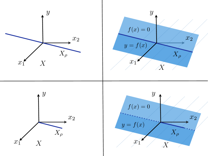
If $K$ separates all possible closed subsets in $X$, we say that it is completely separating. Figure 1 illustrates the notion of separating kernel in the simple example of the linear kernel in a Euclidean space.

Figure 1: The separating property is illustrated in a simple situation where $X={\mathbb{R}^{2}}$. In the top pictures, the support $X_{\rho}$ is a line passing through the origin and is separated by the linear kernel $K(x,y)=x^{T}y$: for all $x\notin X_{\rho}$, there exists a function $f\in\mathcal{H}$ (a linear function on $X$) which is zero on $X_{\rho}$ and such that $f(x)\neq 0$. The pictures on the right are a plot of the plane $y={f(x_{1},x_{2})}$. In the bottom pictures, the support is a segment passing through the origin. The linear kernel is too simple to separate this set: all planes are going to be zero also outside of the support (the dotted line in the picture).

Now, Theorem 3 states that, if either $K$ is completely separating, or at least separates $X_{\rho}$, then $X_{\rho}$ is the level set of a suitable distribution dependent continuous function $F_{\rho}$. More precisely, let ${\mathcal{H}}$ be the reproducing kernel Hilbert space associated to $K$ [2], $T:\mathcal{H}\to\mathcal{H}$ the integral operator with kernel $K$, and denote by $T^{\dagger}$ its pseudo-inverse. If we consider the function $F_{\rho}$ on $X$, defined by

$$F_{\rho}(x)=\left\langle{T^{\dagger}TK_{x}},{K_{x}}\right\rangle\qquad\forall x\in X,$$

and $K$ separates $X_{\rho}$, then we prove that

$$X_{\rho}=\left\{x\in X\mid F_{\rho}(x)=1\right\},$$

(where for simplicity we are assuming $K(x,x)=1$ for all $x\in X$).

The above result is crucial since the integral operator $T$ can be approximated with high probability from data (see [58] and references therein). However, since the definition of $F_{\rho}$ involves the pseudo-inverse of $T$, the support estimation problem can be unstable [71] and regularization techniques are needed to ensure stability. With this in mind, we propose and study a family of spectral regularization techniques which are classical in inverse problems [34] and have been considered in supervised learning in [3, 48]. We define an estimator by

$$X_{n}=\{x\in X~{}|~{}F_{n}(x)\geq 1-\tau_{n}\},$$

where $F_{n}(x)=(1/n){\mathbf{K}}_{{\mathbf{x}}}^{\top}\,g_{\lambda_{n}}({\mathbf{K}_{n}}/n){\mathbf{K}}_{{\mathbf{x}}}$, with ${\mathbf{(}{\mathbf{K}}_{n})}_{i,j}=K(x_{i},x_{j})$, ${\mathbf{K}}_{{\mathbf{x}}}$ is the column vector whose $i$-th entry is $K(x_{i},x)$, and ${\mathbf{K}}_{{\mathbf{x}}}^{\top}$ is its transpose. Here $g_{\lambda_{n}}({\mathbf{K}_{n}}/n)$ is a matrix defined via spectral calculus by a spectral filter function $g_{\lambda_{n}}$ that suppresses the contribution of the eigenvalues smaller than $\lambda_{n}$. Examples of spectral filters include Tikhonov regularization and truncated singular values decomposition [48], to name a few.

This class of methods can be studied within a unified framework, and the error analysis in the paper establishes strong universal consistency if $X_{\rho}$ is separated by $K$. More precisely, under the latter assumption, we show in Theorem 6 that,

$$\lim_{n\to\infty}d_{H}(X_{n},X_{\rho})=0\qquad\text{almost surely},$$

provided that $X$ is compact and the sequences $(\tau_{n})_{n\geq 1},(\lambda_{n})_{n\geq 1}$ are chosen so that,

$${\tau_{n}=1-\min_{1\leq i\leq n}F_{n}(x_{i}),}\quad\quad\lim_{n\to\infty}\lambda_{n}=0,\quad\quad\sup_{n\geq 1}(L_{\lambda_{n}}\log n)/\sqrt{n}<+\infty,$$

where $L_{\lambda_{n}}$ is the Lipschitz constant of the function $r_{\lambda_{n}}(\sigma)=\sigma g_{\lambda_{n}}(\sigma)$. The above result is universal in the sense that consistency can be shown without assuming regularity condition on $\rho$ or $X_{\rho}$.

The proof of the above result crucially depends on estimating the deviation between $F_{n}$ and $F_{\rho}$. Indeed, for the above choice of the sequence $\lambda_{n})_{n\geq 1}$ we show that

$$\lim_{n\to\infty}\sup_{x\in X}\left\lvert{F_{\rho}(x)-F_{n}(x)}\right\rvert=0\qquad\text{almost surely}.$$

Under suitable distribution dependent assumptions, the above result can be further developed to obtain finite sample bounds quantifying stability to random sampling. Indeed, if the couple $(\rho,K)$ is such that $\sup_{x\in X}\left\lVert{T^{-s/2}T^{\dagger}TK_{x}}\right\rVert<+\infty$, with $0<s\leq 1$, and the eigenvalues of the (compact and positive) operator $T$ satisfy $\sigma_{j}\sim j^{-1/b}$ for some $0<b\leq 1$, then we prove in Theorem 7 that, for $n\geq 1$ and $\delta>0$, we have

$$\sup_{x\in X}\left\lvert{F_{n}(x)-F_{\rho}(x)}\right\rvert\leq C_{s,b,\delta}\left(\frac{1}{n}\right)^{\frac{s}{2s+b+1}}$$

with probability at least $1-2e^{-\delta}$, for $\lambda_{n}=n^{-1/(2s+b+1)}$ and a suitable constant $C_{s,b,\delta}$ which does not depend on $n$.

Finally, we remark that our construction relies on the assumption that the kernel $K$ separates the support $X_{\rho}$. The question then arises whether there exist kernels that can separate a large number of, and perhaps all, closed subsets, namely kernels that are completely separating. Indeed, a positive answer can be given and, for translation invariant kernels on $\mathbb{R}^{d}$, Theorem 4 actually gives a sufficient condition for a kernel to be completely separating in terms of its Fourier transform. As a consequence, the Abel kernel $K(x,y)=e^{-\left\lVert{x-y}\right\rVert/\sigma}$ on the Euclidean space $X=\mathbb{R}^{d}$ is completely separating. Interestingly, the Gaussian kernel $K(x,y)=e^{-\left\lVert{x-y}\right\rVert^{2}/\sigma^{2}}$, which is very popular in machine learning, is not.

1.2 State of the art

The problem of building an estimator $X_{n}$ of a subset $X_{\rho}\subset X$ which is consistent with respect to some kind of metric among sets has been considered in seemingly diverse fields for different application purposes, from anomaly detection – see [17] for a review – to surface estimation [60]. We give a summary of the main approaches, with basic references for further details.
Support and Level Set Estimation. Support estimation (also called set estimation) is a part of the theory of non-parametric statistics. We refer to [24, 25] for a detailed review on this topic. Usually, the space $X$ is $\mathbb{R}^{d}$ with the Euclidean metric $d$, and $X_{\rho}$ is the corresponding support of $\rho$. If $X_{\rho}$ is convex, a natural estimator is the convex hull of the data $X_{n}=\operatorname{conv}\left\{x_{1},\ldots,x_{n}\right\}$, for which convergence rates can be derived with respect to the Hausdorff distance [33, 56]. If $X_{\rho}$ is not convex, Devroye and Wise [30] propose the estimator

$$X_{n}=\bigcup_{i=1}^{n}B(x_{i},\epsilon_{n}),$$

where $B(x,\epsilon)$ is the ball of center $x$ and radius $\epsilon$, and $\epsilon_{n}$ slowly goes to zero when $n$ tends to infinity. Consistency and minimax converges rates are studied in [30, 44] with respect to the distance

$$d_{\mu}(C_{1},C_{2})=\mu(C_{1}\triangle C_{2}),$$

where $C_{1}\triangle C_{2}=(C_{1}\setminus C_{2})\cup(C_{2}\setminus C_{1})$ and $\mu$ is a suitable known measure.
If $\rho$ has a density $f$ with respect to some known measure $\mu$, a traditional approach is based on a non-parametric estimator $f_{n}$ of $f$, a so called plug-in estimator. A kernel based class of plug-in estimators is proposed in [23], namely

$${X_{n}=\left\{x\in X\mid f_{n}(x)\geq c_{n}\right\}\quad\text{ with }\quad f_{n}(x)=\frac{1}{nh_{n}^{d}}\sum_{i=1}^{n}K\left(\frac{x-x_{i}}{h_{n}}\right),}$$

where $h_{n}$ is a regularization parameter and $c_{n}$ is a suitable threshold. Convergence rates with respect to $d_{\mu}$ are provided in [23].
A related problem is level set estimation, where the goal is to detect the high density regions $\left\{x\in X\mid f(x)\geq c\right\}$. Consistency and optimal convergence rates for different plug-in estimators

$$X_{n}=\left\{x\in X\mid f_{n}(x)\geq c\right\}$$

have been studied with respect to both $d_{H}$ and $d_{\mu}$, see for example [8, 63, 72] for a slightly different approach.
One class learning algorithm. In machine learning, set estimation has been viewed as a classification problem where we have at our disposal only positive examples. An interesting discussion on the relation between density level set estimation, binary classification and anomaly detection is given in [69]. In this context, some algorithms inspired by Support Vector Machine (SVM) have been studied in [61, 69, 75]. A kernel method based on kernel principal component analysis is presented in [39] and is essentially a special case of our framework.
Manifold Learning. As we mentioned before, a setting which is of special interest is the one in which $X$ is $\mathbb{R}^{d}$ and $X_{\rho}$ is a low dimensional Riemannian submanifold. In this case, the error of an estimator is studied in terms of the error functional

$$d_{\rho}(X_{\rho},X_{n})=\int_{X_{\rho}}d(x,X_{n})d\rho(x),$$

where $d$ is the Euclidean metric. Some results in this framework are given in [1, 49, 51].
Computational Geometry. A classic situation, considered for example in image reconstruction problems, is when the set $X_{\rho}$ is a hyper-surface of $\mathbb{R}^{d}$ and the data $x_{1},\ldots,x_{n}$ are either chosen deterministically or sampled uniformly. The goal in this case is to find a smooth function $f$ that gives the Cartesian equation of the hyper-surface, see for example [40, 42, 47].

2 Kernels, Integral Operators and Geometry in Spaces of Probabilities

In this section we establish the results that provide the foundations of our approach. The basic framework in this paper is described by a triple $(X,\rho,K)$, where

• $X$ is a set (endowed with a $\sigma$-algebra $\mathcal{A}_{X}$);

• $\rho$ is a probability measure defined on $X$;

• $K$ is a (real) reproducing kernel on $X$, i.e. a real function on $X\times X$ of positive type.

We interpret $X$ as the data space and $\rho$ as the probability distribution generating the data. Roughly speaking, the kernel $K$ provides a natural similarity measure on $X$ and it defines its geometry.

We denote by $\mathcal{H}$ the reproducing kernel Hilbert space associated with the reproducing kernel $K$ (we refer to [2, 68] for an exhaustive review on the theory of reproducing kernel Hilbert spaces). The scalar product and norm in $\mathcal{H}$ are denoted by $\left\langle{\cdot},{\cdot}\right\rangle$ and $\left\lVert{\cdot}\right\rVert$, respectively. We recall that the elements of $\mathcal{H}$ are real functions on $X$, and the reproducing property $f(x)=\left\langle{f},{K_{x}}\right\rangle$ holds true for all $x\in X$ and $f\in\mathcal{H}$, where $K_{x}\in\mathcal{H}$ is defined by $K_{x}(y)=K(y,x)$.

In order to prove our results, we need some technical conditions on $K$.

Assumption 1.

The kernel $K$ has the following properties:

1. for all $x,y\in X$ with $x\neq y$ we have $K_{x}\neq K_{y}$;

2. the associated reproducing kernel Hilbert space $\mathcal{H}$ is separable;

3. the real function $K$ is measurable with respect to the product $\sigma$-algebra $\mathcal{A}_{X}\otimes\mathcal{A}_{X}$;

4. for all $x\in X$, $K(x,x)=1$.

Assumptions 1.a), 1.b) and 1.c) are minimal requirements. In particular, Assumptions 1.a) and 1.b) are needed in order to define a separable metric structure on $X$, while Assumption 1.c) ensures that such metric topology is compatible with the $\sigma$-algebra $\mathcal{A}_{X}$ (see Proposition 1 below). In Proposition 2, the combination of 1.a), 1.b) and 1.c) will allow us to define the support $X_{\rho}$ of the probability measure $\rho$, as anticipated in Section 1.1. Assumption 1.d), instead, is a normalization requirement, and could be replaced by a suitable boundedness condition (in fact, even weaker integrability conditions could also be considered). We choose the normalization $K(x,x)=1$ $\forall x\in X$ since it makes equations more readable, and it is not restrictive in view of Proposition 13 in A.1.

We now show how the above assumptions allow us to define a metric on $X$ and to characterize the corresponding support of $\rho$ in terms of the integral operator with kernel $K$.

2.1 Metric induced by a kernel

Our first result makes $X$ a separable metric space isometrically embedded in $\mathcal{H}$. This point of view is developed in [65]. The relation between metric spaces isometrically embedded in Hilbert spaces and kernels of positive type was studied by Schoenberg around 1940. A recent discussion on this topic can be found in Chapter 2 § 3 of [7].

Proposition 1.

Under Assumption 1.a), the map $d_{K}:X\times X\to[0,+\infty[$ defined by

$$d_{K}(x,y)=\left\lVert{K_{x}-K_{y}}\right\rVert=\sqrt{K(x,x)+K(y,y)-{2}K(x,y)}$$ (1)

is a metric on $X$. Furthermore

1. the map $x\mapsto K_{x}$ is an isometry from $X$ into $\mathcal{H}$;

2. the kernel $K$ is a continuous function on $X\times X$, and each $f\in\mathcal{H}$ is a continuous function.

If also Assumption 1.b) is satisfied, then

1. the metric space $(X,d_{K})$ is separable.

Finally, if also Assumption 1.c) holds true, then

1. the closed subsets of $X$ are measurable (with respect to $\mathcal{A}_{X}$);

2. if $Y$ is a topological space endowed with its Borel $\sigma$-algebra and $f:X\to Y$ is continuous, then $f$ is measurable; in particular, the functions in $\mathcal{H}$ are measurable.

Proof.

Many of these properties are known in the literature, see for example [15, 68] and references therein. For the reader’s convenience, we give a self-contained short proof.
Assumption 1.a) states that the map $x\mapsto K_{x}$ is injective. Since $d_{K}(x,y)=\left\lVert{K_{x}-K_{y}}\right\rVert$ by definition, $d_{K}$ is the metric on $X$ making $x\mapsto K_{x}$ an isometry, as claimed in item i). About ii), the kernel $K$ is continuous since $K(x,y)=\left\langle{K_{y}},{K_{x}}\right\rangle$ and the map $x\mapsto K_{x}$ is continuous by item i); furthermore, the elements of $\mathcal{H}$ are continuous by the reproducing property $f(x)=\left\langle{f},{K_{x}}\right\rangle$.
If also Assumption 1.b) holds true, then the set ${\left\{K_{x}\mid x\in X\right\}}$ is separable in $\mathcal{H}$, and so is $X$ as the map $x\mapsto K_{x}$ is isometric from $X$ onto $\left\{K_{x}\mid x\in X\right\}$. Item iii) then follows.
Suppose now that also Assumption 1.c) holds true. Then the map $d_{K}$ is a measurable map, so that the open balls of $X$ are measurable. Since $X$ is separable, any open set is a countable union of open balls, hence it is measurable. It follows that the closed subsets are measurable, too, hence item iv).
Let $Y$ and $f$ be as in item v). If $A\subset Y$ is closed, then $f^{-1}(A)$ is closed in $X$, hence measurable by item iv). It follows that $f^{-1}(A)$ is measurable for all Borel sets $A\subset Y$, i.e. $f$ is measurable. Since the elements of $\mathcal{H}$ are continuous by ii), they are measurable, and item v) is proved. ∎

In the rest of the paper we will always consider $X$ as a topological metric space with metric $d_{K}$. Note that $d_{K}$ is the metric induced on $X$ by the norm of $\mathcal{H}$ through the embedding ${x\mapsto K_{x}}$. The next result shows that under our assumptions we can define the set $X_{\rho}$ as the smallest closed subset of $X$ having measure one.

Proposition 2.

Under Assumptions 1.a), 1.b) and 1.c), there exists a unique closed subset $X_{\rho}\subset X$ with $\rho(X_{\rho})=1$ satisfying the following property: if $C$ is a closed subset of $X$ and $\rho(C)=1$, then $C\supset X_{\rho}$.

Proof.

Define the measurable set $X_{\rho}$ as

$$X_{\rho}=\bigcap_{\begin{smallmatrix}C\text{ \rm closed }\\ \rho(C)=1\end{smallmatrix}}C.$$

Clearly, $X_{\rho}$ is closed and measurable by Proposition 1. Since $X$ is separable, there exists a sequence of closed subsets $(C_{j})_{j\geq 1}$ such that every closed subset $C=\cap C_{j_{k}}$, for some suitable subsequence. Hence, $X_{\rho}=\bigcap\limits_{j\mid\rho(C_{j})=1}C_{j}$ and, as a consequence, $\rho(X_{\rho})=1$. ∎

We add one remark. The set $X_{\rho}$ is called the support of the measure $\rho$ and clearly depends both on the probability distribution and on the topology induced by the kernel $K$ through the metric $d_{K}$ on $X$.

2.2 Separating Kernels

The following definition of separating kernel plays a central role in our approach.

Definition 1.

We say that the reproducing kernel Hilbert space $\mathcal{H}$ separates a subset $C\subset X$, if, for all $x\not\in C$, there exists $f\in\mathcal{H}$ such that

$$f(x)\neq 0\quad\text{ and }\quad f(y)=0\quad\forall y\in C.$$ (2)

In this case we also say that the corresponding reproducing kernel separates $C$.

We add some comments. First, in (2) the function $f$ depends on $x$ and $C$. Second, the reproducing property and (2) imply that $K_{x}\neq 0$ and $K_{x}\neq K_{y}$ for all $x\not\in C$ and $y\in C$ (compare with Assumption 1.a)). Finally, we stress that a different notion of separating property is given in [68].

Remark 1.

Given an arbitrary reproducing kernel Hilbert space $\mathcal{H}$, there exist sets that are not separated by $\mathcal{H}$. For example, if $X=\mathbb{R}^{d}$ and $\mathcal{H}$ is the reproducing kernel Hilbert space with linear kernel $K(x,y)=x^{T}y$, the only sets separated by $\mathcal{H}$ are the linear manifolds, that is, the set of points defined by homogeneous linear equations (see Figure 1). A natural question is then whether there exist kernels capable of separating large classes of subsets and in particular all the closed subsets. Section 3 anwers positively to this question, introducing the notion of completely separating kernels.

Next, we provide an equivalent characterization of the separating property, which will be the key to a computational approach to support estimation. For any set $C$, let $P_{C}:\mathcal{H}\to\mathcal{H}$ be the orthogonal projection onto the closed subspace

$$\mathcal{H}_{C}=\overline{\text{span}\left\{K_{x}\mid x\in C\right\}},$$

i.e. the closure of the linear space generated by the family $\left\{K_{x}\mid x\in C\right\}$. Note that $P_{C}^{2}=P_{C}$, $P_{C}^{\top}=P_{C}$ and

$$\ker{P_{C}}=\left\{K_{x}\mid x\in C\right\}^{\perp}=\{f\in\mathcal{H}\mid f(x)=0\ \forall x\in C\}.$$

Moreover, define the function

$$F_{C}:X\to\mathbb{R},\qquad F_{C}(x)=\left\langle{P_{C}K_{x}},{K_{x}}\right\rangle.$$ (3)

Remark 2.

The Hilbert space $\mathcal{H}_{C}$ is a closed subspace of the reproducing kernel Hilbert space $\mathcal{H}$, and it is itself a reproducing kernel Hilbert space of functions on $X$ with reproducing kernel $K_{C}(x,y)=\left\langle{P_{C}K_{y}},{P_{C}K_{x}}\right\rangle=\left\langle{P_{C}K_{y}},{K_{x}}\right\rangle$. Note that $K_{C}(x,y)=K(x,y)$ for all $x,y\in C$ by definition of $P_{C}$. Clearly, the function $F_{C}$ corresponds to the value of $K_{C}$ on the diagonal.

Then, we have the following theorem.

Theorem 1.

For any subset $C\subset X$, the following facts are equivalent:

1. $\mathcal{H}$ separates the set $C$ ;

2. for all $x\not\in C$, $K_{x}\notin\operatorname{ran}\,P_{C}$;

3. $\displaystyle{C=\left\{x\in X\mid F_{C}(x)=K(x,x)\right\}}$;

4. $\displaystyle{{\left\{K_{x}\mid x\in C\right\}=\left\{K_{x}\mid x\in X\right\}}\cap\operatorname{ran}\,P_{C}}$.

Under Assumption $\ref{A}.\ref{A3})$, if $C$ is separated by $\mathcal{H}$, then $C$ is closed with respect to the metric $d_{K}$.

Proof.

We first prove that i) $\Rightarrow$ ii). Given $x\notin C$, by assumption there is $f\in\mathcal{H}$ such that $\left\langle{f},{K_{x}}\right\rangle=f(x)\neq 0$, i.e. $K_{x}\not\in\left\{f\right\}^{\perp}$, and $\left\langle{f},{K_{y}}\right\rangle=f(y)=0$ for all $y\in C$, i.e. $f\in\ker{P_{C}}=\operatorname{ran}\,P_{C}^{\perp}$. It follows that $\operatorname{ran}\,P_{C}\subset\left\{f\right\}^{\perp}$, and then $K_{x}\notin\operatorname{ran}\,P_{C}$.
We prove ii) $\Rightarrow$ iii). If $x\in C$, then $K_{x}\in\operatorname{ran}\,P_{C}$ by definition of $P_{C}$, so that $F_{C}(x)=K(x,x)$. Hence $C\subset\left\{x\in X\mid F_{C}(x)=K(x,x)\right\}$. If $x\not\in C$, then by assumption $P_{C}K_{x}\neq K_{x}$, i.e. $(I-P_{C})K_{x}\neq 0$. By the equality

$$\left\lVert{(I-P_{C})K_{x}}\right\rVert^{2}=\left\langle{K_{x}},{K_{x}}\right\rangle-\left\langle{P_{C}K_{x}},{K_{x}}\right\rangle-\left\langle{K_{x}},{P_{C}K_{x}}\right\rangle+\left\langle{P_{C}K_{x}},{P_{C}K_{x}}\right\rangle=K(x,x)-F_{C}(x),$$

this implies $F_{C}(x)\neq K(x,x)$. Hence $C\supset\left\{x\in X\mid F_{C}(x)=K(x,x)\right\}$.
We prove iii) $\Rightarrow$ i). If $x\not\in C$, define $f=(I-P_{C})K_{x}\in\ker{P_{C}}$, so that $f(y)=0$ for all $y\in C$. Furthermore, $f(x)=K(x,x)-F_{C}(x)\neq 0$. Thus, $f$ separates the set $C$.
Finally, iv) is a restatement of ii) taking into account that $K_{x}\in\operatorname{ran}\,P_{C}$ for all $x\in C$ by construction.
Under Assumption $\ref{A}.\ref{A3})$, the map $x\mapsto F_{C}(x)-K(x,x)=\left\langle{P_{C}K_{x}},{K_{x}}\right\rangle-K(x,x)$ is continuous by Proposition 1. By item iii), $C$ is the $0$-level set of this function, hence $C$ is closed. ∎

Proposition 13 in A.1 shows that the reproducing kernel $K$ can be normalized under the mild assumption that $K(x,x)\neq 0$ for all $x\in X$, so that Assumption 1.d) can be satisfied up to a rescaling of $K$.

2.2.1 A Special Case: Metric Spaces

It may be the case that the set $X$ has its own metric $d_{X}$, and the $\sigma$-algebra $\mathcal{A}_{X}$ is the Borel $\sigma$-algebra associated with the topology induced by $d_{X}$. The following proposition shows that the metrics $d_{K}$ and $d_{X}$ induce the same topology on $X$, provided that $\mathcal{H}$ separates all the $d_{X}$-closed subsets and the corresponding kernel is continuous.

Proposition 3.

Let $X$ be a separable metric space with respect to a metric $d_{X}$, and $\mathcal{A}_{X}$ the corresponding Borel $\sigma$-algebra. Let $\mathcal{H}$ be a reproducing kernel Hilbert space on $X$ with kernel $K$. Assume that the kernel $K$ is a continuous function with respect to $d_{X}$ and that the space $\mathcal{H}$ separates every subset of $X$ which is closed with respect to $d_{X}$. Then

1. Assumptions $\ref{A}.\ref{A3})$, $\ref{A}.\ref{A1})$ and $\ref{A}.\ref{A2})$ hold true, and $K(x,x)>0$ for all $x\in X$;

2. a set is closed with respect to $d_{K}$ if and only if it is closed with respect to $d_{X}$.

Proof.

The kernel is measurable and the space $\mathcal{H}$ is separable by Proposition $5.1$ and Corollary $5.2$ in [15]. Since the points are closed sets for $d_{X}$ and the $d_{X}$-closed sets are separated by $\mathcal{H}$, then $K_{x}\neq 0$ (i.e. $K(x,x)>0$) for all $x\in X$ and $K_{x}\neq K_{y}$ if $x\neq y$ by the discussion following Definition 1.
We show that $d_{X}$ and $d_{K}$ are equivalent metrics. Take a sequence $(x_{j})_{j\geq 1}$ such that for some $x\in X$ it holds that $\lim_{j\to\infty}d_{X}(x_{j},x)=0$. Since $K$ is continuous with respect to $d_{X}$, we have $\lim_{j\to\infty}d_{K}(x_{j},x)=0$. Hence, the $d_{K}$-closed sets are $d_{X}$-closed, too. Conversely, if the set $C$ is $d_{X}$-closed, since $\mathcal{H}$ separates $C$, Theorem 1 implies that $C=\left\{x\in X\mid K(x,x)-F_{C}(x)=0\right\}$, which is a $d_{K}$-closed set by $d_{K}$-continuity of the map $x\mapsto K(x,x)-F_{C}(x)$. ∎

Item ii) of the above proposition states that the metrics $d_{K}$ and $d_{X}$ are equivalent and implies that the set $X_{\rho}$ defined in Proposition 2 coincides with the support of $\rho$ with respect to the topology induced by $d_{X}$.

2.3 The Integral Operator Defined by the Kernel

We denote by $\mathcal{S}_{1}$ the Banach space of the trace class operators on $\mathcal{H}$, with trace class norm

$$\left\lVert{A}\right\rVert_{\mathcal{S}_{1}}=\operatorname{tr}\left[(A^{\top}A)^{\frac{1}{2}}\right]=\sum_{i\in I}\left\langle{(A^{\top}A)^{\frac{1}{2}}e_{i}},{e_{i}}\right\rangle,$$

where $\left\{e_{i}\right\}_{i\in I}$ is any orthonormal basis of $\mathcal{H}$. Furthermore, we let $\mathcal{S}_{2}$ be the separable Hilbert space of the Hilbert-Schmidt operators on $\mathcal{H}$, with Hilbert-Schmidt norm

$$\left\lVert{A}\right\rVert^{2}_{\mathcal{S}_{2}}=\operatorname{tr}\left[A^{\top}A\right]=\sum_{i\in I}\left\lVert{Ae_{i}}\right\rVert^{2}.$$

Finally, if $A$ is any bounded operator on $\mathcal{H}$, we denote by $\left\lVert{A}\right\rVert_{\infty}$ its uniform operator norm. It is standard that $\left\lVert{A}\right\rVert_{\infty}\leq\left\lVert{A}\right\rVert_{\mathcal{S}_{2}}\leq\left\lVert{A}\right\rVert_{\mathcal{S}_{1}}$. Moreover, for all functions $f_{1},f_{2}\in\mathcal{H}$, the rank-one operator $f_{1}\otimes f_{2}$ on $\mathcal{H}$ defined by

$$(f_{1}\otimes f_{2})(f)=\left\langle{f},{f_{2}}\right\rangle\,f_{1}\qquad\forall f\in\mathcal{H}$$

is trace class, and $\left\lVert{f_{1}\otimes f_{2}}\right\rVert_{\mathcal{S}_{1}}=\left\lVert{f_{1}\otimes f_{2}}\right\rVert_{\mathcal{S}_{2}}=\left\lVert{f_{1}}\right\rVert\left\lVert{f_{2}}\right\rVert$.

We recall a few facts on integral operators with kernel $K$ (see [15] for proofs and further discussions). Under Assumption 1, the $\mathcal{S}_{1}$-valued map $x\mapsto K_{x}\otimes K_{x}$ is Bochner-integrable with respect to $\rho$, and its integral

$$T{=}\int_{X}K_{x}\otimes K_{x}d\rho(x)$$ (4)

defines a positive trace class operator $T$ with $\left\lVert{T}\right\rVert_{\mathcal{S}_{1}}=\operatorname{tr}\left[T\right]=1$ (a short proof is given in Proposition 14 of the Appendix). Using the reproducing property of $\mathcal{H}$, it is straightforward to see that $T$ is simply the integral operator with kernel $K$ acting on $\mathcal{H}$, i.e.

$$(Tf)(x)=\int_{X}K(x,y)f(y)d\rho(y)\qquad\forall f\in\mathcal{H}.$$

The following is a key result in our approach.

Theorem 2.

Under Assumption 1, the null space of $T$ is

$$\ker{T}=\left\{K_{x}\mid x\in X_{\rho}\right\}^{\perp}=\ker{P_{X_{\rho}}},$$ (5)

where $X_{\rho}$ is the support of $\rho$ as defined in Proposition 2.

Proof.

Note that , for all $f\in\mathcal{H}$, the set

$$C_{f}=\left\{x\in X\mid f(x)=0\right\}=\left\{x\in X\mid\left\langle{f},{K_{x}}\right\rangle=0\right\}$$

is closed since $f$ is continuous. We now prove Equation (5). Since $T$ is a positive operator, spectral theorem gives that $Tf=0$ if and only if $\left\langle{Tf},{f}\right\rangle=0$. The definition of $T$ and the reproducing property gives that

$$\left\langle{Tf},{f}\right\rangle=\int_{X}\left\langle{(K_{x}\otimes K_{x})f},{f}\right\rangle d\rho(x)=\int_{X}\left\lvert{\left\langle{K_{x}},{f}\right\rangle}\right\rvert^{2}d\rho(x)=\int_{X}|f(x)|^{2}d\rho(x),$$

hence the condition $\left\langle{Tf},{f}\right\rangle=0$ is equivalent to the fact that $f(x)=0$ for $\rho$-almost every $x\in X$. Hence $f\in\ker{T}$ if and only if $\rho(C_{f})=1$, i.e. $C_{f}\supset X_{\rho}$, or equivalently $\left\langle{f},{K_{x}}\right\rangle=0$ $\forall x\in X_{\rho}$. Equation (5) then follows. ∎

In the following, we will use the abbreviated notation $P_{\rho}=P_{X_{\rho}}$. Note that the space $\mathcal{H}$ splits into the direct sum $\mathcal{H}=\mathcal{H}_{\rho}\oplus\mathcal{H}_{\rho}^{\perp}$, where

$$\mathcal{H}_{\rho} ={\operatorname{ran}\,P_{\rho}=\overline{\operatorname{ran}\,T}=\overline{\text{span}\{K_{x}\mid x\in X_{\rho}\}}}$$

$$\mathcal{H}_{\rho}^{\perp} =\ker{P_{\rho}}=\ker{T}=\{f\in\mathcal{H}\mid f(x)=0\ \forall x\in X_{\rho}\}.$$

Remark 3.

The reproducing kernel Hilbert space $\mathcal{H}_{\rho}$ (see Remark 2) has been considered before [70], and in particular in the context of semi-supervised manifold regularization [5], where $X_{\rho}$ is assumed to be an embedded manifold. The corresponding reproducing kernel is $K_{\rho}(x,y)=\left\langle{P_{\rho}K_{y}},{K_{x}}\right\rangle$ and $F_{X_{\rho}}(x)=K_{\rho}(x,x)$. See also the discussion in Section 6.

Under Assumption 1, we also introduce the integral operator $L_{K}:L^{2}(X,\rho)\to L^{2}(X,\rho)$,

$$(L_{K}\phi)(x){=}\int_{X}K(x,y)\phi(y)d\rho(y)\qquad\forall\phi\in L^{2}(X,\rho),$$

which is a positive trace class operator, too. Note the difference between the operators $T$ and $L_{K}$: although their definitions are formally the same, the respective domains and images change.

Since $T$ and $L_{K}$ are positive trace class operators, by the Hilbert-Schmidt theorem each of them admits an orthonormal family of eigenvectors in $\mathcal{H}$ and $L^{2}(X,\rho)$, respectively, with a corresponding family of positive eigenvalues. The two spectral decompositions are strongly related, as we now briefly recall (see also Proposition 8 of [58] and Theorem 2.11 of [70]).

Denote by $(\sigma_{j})_{j\in J}$ the (finite or countable) family of strictly positive eigenvalues of $L_{K}$, where each eigenvalue is repeated according to its (finite) multiplicity. For each $j\in J$ select a corresponding eigenvector $\phi_{j}\in L^{2}(X,\rho)$ in such a way that the sequence $(\phi_{j})_{j\in J}$ is orthonormal in $L^{2}(X,\rho)$. Hilbert-Schmidt theorem provides that

$$L_{K}=\sum_{j\in J}\sigma_{j}\phi_{j}\otimes\phi_{j},$$ (6)

where the series converges in trace norm. In general, each element $\phi_{j}$ is an equivalence class of functions defined $\rho$-almost everywhere. In particular, the value of $\phi_{j}$ is not defined outside $X_{\rho}$. However, in each equivalence class we can choose a unique continuous function, denoted again by $\phi_{j}$, which is defined at every point of $X$ by means of the extension equation [19, 58]

$$\phi_{j}(x)=\sigma_{j}^{-1}\int_{X}K(x,y)\phi_{j}(y)d\rho(y)\qquad\forall x\in X.$$ (7)

With this choice, which will be implicitly assumed in the following, the family $(\sigma_{j})_{j\in J}$ coincides with the family of strictly positive eigenvalues of $T$ (with the same multiplicities), $(\sqrt{\sigma_{j}}\phi_{j})_{j\in J}$ is a orthonormal family in $\mathcal{H}$ of eigenfunctions of $T$, and

$$T=\sum_{j\in J}\sigma_{j}\,\,(\sqrt{\sigma_{j}}\phi_{j})\otimes(\sqrt{\sigma_{j}}\phi_{j})=\sum_{j\in J}\sigma_{j}^{2}\ \phi_{j}\otimes\phi_{j},$$ (8)

where the series converges in the Banach space $\mathcal{S}_{1}$ (hence in $\mathcal{S}_{2}$), see e.g. [15, 58, 70]. As $\left\lVert{T}\right\rVert_{\mathcal{S}_{1}}=1$, the positive sequence $(\sigma_{j})_{j\in J}$ is summable and sums up to $1$. It is clear that the family $(\sqrt{\sigma_{j}}\phi_{j})_{j\in J}$ is an orthonormal basis of the Hilbert space $\mathcal{H}_{\rho}$. Conversely, let $(f_{j})_{j\in J}$ be an orthonormal basis of $\mathcal{H}_{\rho}$ of eigenvectors of $T$ with corresponding eigenvalues $(\sigma_{j})_{j\in J}$. Define

$$\phi_{j}(x)=\sigma_{j}^{-\frac{1}{2}}f_{j}(x)\qquad\forall x\in X{.}$$

Then, it is not difficult to show that (6), (7) and (8) hold true.

2.4 An Analytic Characterization of the Support

Let Assumption 1 hold true. Collecting the previous results, if $\mathcal{H}$ separates $X_{\rho}$, then Theorem 1 gives that

$$X_{\rho}=\left\{x\in X\mid F_{X_{\rho}}(x)=1\right\}.$$

The function $F_{\rho}=F_{X_{\rho}}$ is defined by (3) in terms of the projection $P_{\rho}$, which, in light of Theorem 2, can be characterized using the operator $T$. Indeed, from the definition of $F_{\rho}$ and (5) we have

$${F_{\rho}(x)=}\left\langle{P_{\rho}K_{x}},{K_{x}}\right\rangle=\left\langle{T^{\dagger}TK_{x}},{K_{x}}\right\rangle=\left\langle{\theta(T)K_{x}},{K_{x}}\right\rangle=\sum_{j\in J}{\sigma_{j}\left\lvert{\phi_{j}(x)}\right\rvert^{2}}$$ (9)

where $T^{\dagger}$ is the pseudo-inverse of $T$ and $\theta$ is the Heaviside function $\theta(\sigma)=1{\hskip-2.5pt}\hbox{I}_{]0,+\infty[}(\sigma)$ (note that with our definition $\theta(0)=0)$. The above discussion is summarized in the following theorem.

Theorem 3.

If $\mathcal{H}$ satisfies Assumption 1 and separates the support $X_{\rho}$ of the measure $\rho$, then

$$X_{\rho}=\left\{x\in X\mid F_{\rho}(x)=1\right\}=\left\{x\in X\mid\left\langle{T^{\dagger}TK_{x}},{K_{x}}\right\rangle=1\right\}.$$

As we discussed before, a natural question is whether there exist kernels capable to separate all possible closed subsets of $X$. In a learning scenario, this can be translated into a universality property, in the sense that it allows to describe any probability distribution and learn consistently its support [29]. Note that in a supervised learning framework a similar role is played by the so called universal kernels [16, 67]. The following section answers positively to the previous question, introducing and studying the concept of completely separating kernels. Interestingly, there are universal kernels in the sense of [16, 67] which do not separate all closed subsets of $X$, as for example the Gaussian kernel.

3 Completely separating reproducing kernel Hilbert spaces

The property defining the class of kernels we are interested in is captured by the following definition.

Definition 2 (Completely Separating Kernel).

A reproducing kernel Hilbert space $\mathcal{H}$ satisfying Assumption $\ref{A}.\ref{A3})$ is called completely separating if $\mathcal{H}$ separates all the subsets $C\subset X$ which are closed with respect to the metric $d_{K}$ defined by (1). In this case, we also say that the corresponding reproducing kernel is completely separating.

The definition of completely separating reproducing kernel Hilbert spaces should be compared with the analogous notion of complete regularity for topological spaces. Indeed, we recall that a topological space is called completely regular if, for any closed subset $C$ and any point $x\notin C$, there exists a continuous function $f$ such that $f(x)\neq 0$ and $f(y)=0$ for all $y\in C$. As we discuss below, completely separating reproducing kernels do exist. For example, for $X=\mathbb{R}^{d}$ both the Abel kernel $K(x,y)=e^{-\left\lVert{x-y}\right\rVert/\sigma}$ and the $\ell_{1}$-exponential kernel $K(x,y)=e^{-\left\lVert{x-y}\right\rVert_{1}/\sigma}$ are completely separating, where $\left\lVert{x}\right\rVert$ is just the Euclidean norm of $x=(x^{1},\dots,x^{d})$ in $\mathbb{R}^{d}$ and $\left\lVert{x}\right\rVert_{1}=\sum_{j=1}^{d}|x_{j}|$ is the $\ell_{1}$-norm. Indeed this follows from Theorem  4 and Proposition 6 below, which give sufficient conditions for a kernel to be completely separating in the case $X=\mathbb{R}^{d}$. Note that the Gaussian kernel $K(x,y)=e^{-\left\lVert{x-y}\right\rVert^{2}/\sigma^{2}}$ on $\mathbb{R}^{d}$ is not completely separating. This is a consequence of the following fact. It is known that the elements of the corresponding reproducing kernel Hilbert space $\mathcal{H}$ are analytic functions, see Corollary 4.44 in [68]. If $C$ is a closed subset of $\mathbb{R}^{d}$ with non-empty interior and $f\in\mathcal{H}$ is equal to zero on $C$, then a standard result in complex analysis implies that $f(x)=0$ for all $x\in\mathbb{R}^{d}$, hence $\mathcal{H}$ does not separate $C$.

We end this section with Proposition 6, which gives a simple way to build completely separating kernels in high dimensional spaces from completely separating kernels in one dimension, the latter usually being easier to characterize.

3.1 Separating Properties of Translation Invariant Kernels

The first result studies translation invariant kernels on $\mathbb{R}^{d}$, i.e. of the form $K(x,y)=K(x-y)$. We show that if the Fourier transform of the kernel satisfies a suitable growth condition, then the corresponding reproducing kernel Hilbert space is completely separating. As usual, $C(\mathbb{R}^{d})$ denotes the space of real continuous functions on $\mathbb{R}^{d}$ and, for any $p\in[1,+\infty\,[$, $L^{p}(\mathbb{R}^{d})$ is the space of (equivalence classes of) real functions on $\mathbb{R}^{d}$ which are $p$-integrable with respect to the Lebesgue measure $dx$. We will consider the real spaces $L^{p}_{h}(\mathbb{R}^{d})$ of hermitian complex functions, i.e.

$$L^{p}_{h}(\mathbb{R}^{d})=\{\phi_{1}+i\phi_{2}\mid\phi_{1},\phi_{2}\in L^{p}(\mathbb{R}^{d})\mbox{ and }\phi_{1}(-x)=\phi_{1}(x)\,,\,\phi_{2}(-x)=-\phi_{2}(x)\}.$$

If $\phi\in L^{1}(\mathbb{R}^{d})$, its Fourier transform is the complex hermitian bounded continuous function $\hat{\phi}$ on $\mathbb{R}^{d}$ given by

$$\hat{\phi}(z)=\int_{\mathbb{R}^{d}}e^{-2\pi iz\cdot x}\phi(x)dx.$$

If $\phi\in L^{2}(\mathbb{R}^{d})$, we denote by $\hat{\phi}\in L^{2}_{h}(\mathbb{R}^{d})$ its Fourier-Plancherel transform, obtained extending the above definition on functions $\phi\in L^{1}(\mathbb{R}^{d})\cap L^{2}(\mathbb{R}^{d})$ to a unitary map $L^{2}(\mathbb{R}^{d})\ni\phi\to\hat{\phi}\in L^{2}_{h}(\mathbb{R}^{d})$.

Throughout, we assume $\mathbb{R}^{d}$ to be a metric space with respect to the standard metric $d_{\mathbb{R}^{d}}$ induced by the Euclidean norm.

We need a preliminary result characterizing a reproducing kernel Hilbert space, whose reproducing kernel is continuous and integrable, as a suitable non-closed subspace of $L^{2}(\mathbb{R}^{d})$. The first part is a converse of Bochner’s theorem (Theorem 4.18 in [35]).

Proposition 4.

Let $K$ be a continuous function in $L^{1}(\mathbb{R}^{d})$ such that its Fourier transform $\hat{K}$ is strictly positive. Then the kernel $K(x,y)=K(x-y)$ is positive definite and its corresponding (real) reproducing kernel Hilbert space $\mathcal{H}$ is

$${\mathcal{H}=\left\{\phi\in C(\mathbb{R}^{d})\cap L^{2}(\mathbb{R}^{d})\mid\int_{\mathbb{R}^{d}}\hat{K}(z)^{-1}|\hat{\phi}(z)|^{2}dz<+\infty\right\}}$$ (10)

with norm

$$\left\lVert{\phi}\right\rVert^{2}=\int_{\mathbb{R}^{d}}\hat{K}(z)^{-1}|\hat{\phi}(z)|^{2}dz\qquad\forall\phi\in\mathcal{H}.$$ (11)

Proof.

The integral operator

$$({L_{K}}\phi)(x)=\int_{\mathbb{R}^{d}}K(x-y)\phi(y)\,dy=(K*\phi)(x),$$

is well defined and bounded from $L^{2}(\mathbb{R}^{d})$ into $L^{2}(\mathbb{R}^{d})$ since $K\in L^{1}(\mathbb{R}^{d})$. Since ${L_{K}}$ is a convolution operator, Fourier transform turns it into the operator of multiplication by the bounded function $\hat{K}$, that is $\widehat{{L_{K}}\phi}=\hat{K}\hat{\phi}$ for all $\phi\in L^{2}(\mathbb{R}^{d})$. It follows that

$$\left\langle{{L_{K}}\phi},{\phi}\right\rangle_{L^{2}}=\left\langle{\hat{K}\hat{\phi}},{\hat{\phi}}\right\rangle_{L^{2}}{>0\qquad\forall\phi\in L^{2}(\mathbb{R}^{d})\setminus\{0\}}$$

since $\hat{K}>0$ by assumption, hence ${L_{K}}$ is a strictly positive operator. In order to show that $K$ is positive definite, pick a Dirac sequence $(\varphi_{n})_{n\geq 1}$ as in Chapter VIII.3 of [45], and, for each $x\in X$, define $\varphi_{n}^{x}$ be equal to $\varphi_{n}^{x}(y)=\varphi_{n}(y-x)$. Fixed $x_{1},x_{2},\ldots,x_{N}\in\mathbb{R}^{d}$ and $c_{1},c_{2},\ldots,c_{N}\in{\mathbb{R}}$, set $\phi_{n}=\sum_{i=1}^{N}c_{i}\varphi_{n}^{x_{i}}$, then

$$0\leq\left\langle{{L_{K}}\phi_{n}},{\phi_{n}}\right\rangle_{L^{2}}=\sum_{i,j=1}^{N}c_{i}{c_{j}}\left\langle{{L_{K}}\varphi_{n}^{x_{i}}},{\varphi_{n}^{x_{j}}}\right\rangle_{L^{2}}\mathop{\longrightarrow}_{n\to\infty}\,\sum_{i,j=1}^{N}c_{i}{c_{j}}K(x_{j},x_{i}),$$

where the last equality is due to continuity of $K$ and the usual properties of Dirac sequences. It follows that $\sum_{i,j=1}^{N}c_{i}{c_{j}}K(x_{j},x_{i})\geq 0$, i.e. the kernel $K$ is positive definite.
Let $\mathcal{H}$ be the (real) reproducing kernel Hilbert space associated to $K$. Since the support of the Lebesgue measure is $\mathbb{R}^{d}$, Mercer theorem (as stated e.g. in Proposition 6.1 of [15] and the subsequent discussion, or Theorem 2.11 of [70]) shows that ${L_{K}}^{1/2}$ is a unitary isomorphism from $L^{2}(\mathbb{R}^{d})$ onto $\mathcal{H}$. More precisely, for any $\psi\in L^{2}(\mathbb{R}^{d})$ there exists a unique function $\phi\in C(\mathbb{R}^{d})$ such that its equivalence class belongs to ${L_{K}}^{1/2}\psi\in L^{2}(\mathbb{R}^{d})$, and the correspondence $\psi\mapsto\phi$ is an isometry from $L^{2}(\mathbb{R}^{d})$ onto $\mathcal{H}$. By further applying the Fourier-Plancherel transform and taking into account that $\hat{\phi}(z)=\sqrt{\hat{K}(z)}\,\hat{\psi}(z)$ for almost all $z\in\mathbb{R}^{d}$, one has

$$\left\lVert{\phi}\right\rVert^{2}_{\mathcal{H}}=\left\lVert{\psi}\right\rVert^{2}_{L^{2}(\mathbb{R}^{d})}=\left\lVert{\hat{\psi}}\right\rVert^{2}_{L^{2}_{h}(\mathbb{R}^{d})}=\int_{\mathbb{R}^{d}}\hat{K}(z)^{-1}|\hat{\phi}(z)|^{2}dz<+\infty,$$

so that (10) and (11) follow. ∎

We now state a sufficient condition on $K$ ensuring that $\mathcal{H}$ is completely separating.

Theorem 4.

Let $K$ be a continuous function in $L^{1}(\mathbb{R}^{d})$ such that

$$\hat{K}(z)\geq\frac{a}{\left(1+b\left\lVert{z}\right\rVert^{\gamma_{1}}\right)^{\gamma_{2}}}\qquad\forall y\in\mathbb{R}^{d}$$ (12)

for some $a,b,\gamma_{1},\gamma_{2}>0$. Then,

1. the translation invariant kernel $K(x,y)=K(x-y)$ is positive definite and continuous;

2. the topologies induced by the metric $d_{K}$ and the Euclidean metric $d_{\mathbb{R}^{d}}$ coincide on $\mathbb{R}^{d}$;

3. the kernel $K$ is completely separating.

Proof.

Condition (12) implies that $\hat{K}$ is strictly positive, so item i) follows from Proposition 4. In particular, from (10) we see that, if $\phi\in L^{2}(\mathbb{R}^{d})$ and $\int_{\mathbb{R}^{d}}\left(1+b\left\lVert{z}\right\rVert^{\gamma_{1}}\right)^{\gamma_{2}}|\hat{\phi}(z)|^{2}dz$ is finite, then $\phi\in\mathcal{H}$. This implies that $C^{\infty}_{c}(\mathbb{R}^{d})\subset\mathcal{H}$: indeed, if $\phi\in C^{\infty}_{c}(\mathbb{R}^{d})$, then $\hat{\phi}$ is a Schwartz function on $\mathbb{R}^{d}$ (Theorem 3.2 in [66]), hence the last integral is convergent. Functions in $C^{\infty}_{c}(\mathbb{R}^{d})$ separate every set $C$ which is closed with respect to the metric $d_{\mathbb{R}^{d}}$ (as it easily follows by suitably translating and dilating the function $\psi\in C^{\infty}_{c}(\mathbb{R}^{d})$ defined in item (b) p. 19 of [66]), hence $\mathcal{H}$ separates the $d_{\mathbb{R}^{d}}$-closed subsets. Items ii) and iii) then follow from Proposition 3. ∎

As an application, we show that the Abel kernel is completely separating.

Proposition 5.

Let

$$K:\mathbb{R}^{d}\times\mathbb{R}^{d}\to\mathbb{R},\qquad K(x,y)=e^{-\frac{\left\lVert{x-y}\right\rVert}{\sigma}},$$ (13)

with $\sigma>0$. Then $K$ is a positive definite kernel and the corresponding reproducing kernel Hilbert space $\mathcal{H}$ is completely separating for all $d\geq 1$.

Proof.

A standard Fourier transform computation gives

$$\hat{K}(z)=\frac{1}{2\pi\sigma}\pi^{-\frac{d+1}{2}}\Gamma\left(\frac{d+1}{2}\right)\left(\frac{1}{4\pi^{2}\sigma^{2}}+\left\lVert{z}\right\rVert^{2}\right)^{-\frac{d+1}{2}},$$ (14)

where $\Gamma$ is Euler gamma function (Theorem 1.14 in [66]). The claim then follows from Theorem 4. ∎

Equations (10), (11) and (14) show that (up to a rescaling of the norm) the reproducing kernel Hilbert space associated to the Abel Kernel (13) is just $W^{(d+1)/2}(\mathbb{R}^{d})$, the Sobolev space of order $(d+1)/2$.

3.2 Building Separating Kernels

The following result gives a way to construct completely separating reproducing kernel Hilbert spaces on high dimensional spaces.

Proposition 6.

If $X_{i}$, $i=1,2\ldots d$, are sets and $K^{(i)}$ are completely separating reproducing kernels on $X_{i}$ for all $i=1,2\ldots d$, then the product kernel

$$K((x_{1},\ldots,x_{d}),(y_{1},\ldots,y_{d})){=}K^{(1)}(x_{1},y_{1})\cdots K^{(d)}(x_{d},y_{d})$$

is completely separating on the set $X=X_{1}\times X_{2}\times\ldots\times X_{d}$.

Proof.

Each set $X_{i}$ and $X$ are endowed with the metric $d_{K^{(i)}}$ and $d_{K}$ induced by the corresponding kernels, and $\mathcal{H}_{i}$ and $\mathcal{H}$ denote the reproducing kernel Hilbert spaces with kernels $K^{(i)}$ and $K$, respectively. A standard result gives that $\mathcal{H}=\mathcal{H}_{1}\otimes\ldots\otimes\mathcal{H}_{d}$ and $K_{x}=K^{(1)}_{x_{1}}\otimes\ldots\otimes K^{(d)}_{x_{d}}$ for all $x=(x_{1},\ldots,x_{d})\in X$ [2] . We claim that the $d_{K}$-topology on $X$ is contained in the product topology of the $d_{K^{(i)}}$-topologies on $X_{i}$ (actually, it is not difficult to show that the two topologies coincide). Indeed, if $(x_{i,k})_{k\geq 1}$ are sequences in $X_{i}$ such that $\lim_{k\to\infty}d_{K^{(i)}}(x_{i,k},x_{i})=0$ for all $i=1,\ldots,d$, then

$$\lim_{k\to\infty}d_{K}\left((x_{1,k},\ldots,x_{d,k}),(x_{1},\ldots,x_{d})\right)^{2}=\lim_{k\to\infty}\left\lVert{K_{(x_{1,k},\ldots,x_{d,k})}-K_{(x_{1},\ldots,x_{d})}}\right\rVert^{2}$$

$$\qquad\quad=\lim_{k\to\infty}[K^{(1)}(x_{1,k},x_{1,k})\cdots K^{(d)}(x_{d,k},x_{d,k})-{2}\,K^{(1)}(x_{1,k},x_{1})\cdots K^{(d)}(x_{d,k},x_{d})$$

$$\qquad\qquad+K^{(1)}(x_{1},x_{1})\cdots K^{(d)}(x_{d},x_{d})]$$

$$\qquad\quad=0,$$

since $\lim_{k\to\infty}K^{(i)}(x_{i,k},x_{i,k})=\lim_{k\to\infty}K^{(i)}(x_{i,k},x_{i})=K^{(i)}(x_{i},x_{i})$. We now prove that $\mathcal{H}$ is completely separating. If $C\subset X$ is $d_{K}$-closed and $x=(x_{1},\ldots,x_{d})\in X\setminus C$, since $C$ is also closed in the product topology, for all $i=1,\ldots,d$ there exists an open neighborhood $U_{i}$ of $x_{i}$ in $X_{i}$ such that $U=U_{1}\times\ldots\times U_{d}\subset X\setminus C$. Since each $\mathcal{H}_{i}$ is completely separating, for all $i=1,\ldots,d$ there exists $f_{i}\in\mathcal{H}_{i}$ such that $f_{i}(x_{i})\neq 0$ and $f_{i}(y_{i})=0$ for all $y_{i}\in X_{i}\setminus U_{i}$. Then the product function $f=f_{1}\otimes\ldots\otimes f_{d}$ is in $\mathcal{H}$, and satisfies $f(x)\neq 0$ and $f(y)=0$ for all $y\in C$. ∎

As a consequence, the Abel kernel defined by the $\ell_{1}$-norm

$$K(x,y)=e^{-\frac{\left\lVert{x-y}\right\rVert_{1}}{\sigma}}=\prod_{i=1}^{d}\,e^{-\frac{\left\lvert{x_{i}-y_{i}}\right\rvert}{\sigma}},\qquad x=(x_{1},\ldots,x_{d}),\,y=(y_{1},\ldots,y_{d})$$

is completely separating since each kernel in the product is positive definite and completely separating by Proposition 5.

4 A Spectral Approach to Learning the Support

In this section we study the set estimation problem in the context of learning theory. We fix a triple $(X,\rho,K)$ as in Section 2, and assume throughout that the reproducing kernel $K$ satisfies Assumption 1. We regard $X$ as a metric space with respect to $d_{K}$, and continue to denote by $X_{\rho}$ the support of $\rho$ defined in Proposition 2.

If $\mathcal{H}$ separates $X_{\rho}$, Theorem 3 shows that the support $X_{\rho}$ is the $1$-level set of a suitable function $F_{\rho}$ defined by the integral operator $T$, and therefore depending on $K$ and $\rho$. However, the probability distribution $\rho$ is unknown, as we only have a set of i.i.d. points $x_{1},\dots,x_{n}$ sampled from $\rho$ at our disposal. Our task is now to use our sample in order to estimate the set $X_{\rho}$.

The definition of $T$ given by (4) suggests that it can be estimated by the data dependent operator

$$T_{n}=\frac{1}{n}\sum_{i=1}^{n}K_{x_{i}}\otimes K_{x_{i}}.$$ (15)

The operator $T_{n}$ is positive and with finite rank; in particular, $T_{n}\in\mathcal{S}_{1}$ and $\left\lVert{T_{n}}\right\rVert_{\mathcal{S}_{1}}=\operatorname{tr}\left[T_{n}\right]=1$. We denote by $(\sigma^{(n)}_{j})_{j\in J_{n}}$ the strictly positive eigenvalues of $T_{n}$ (each one repeated according to its multiplicity) and by $\big{(}\sqrt{\sigma^{(n)}_{j}}\phi^{(n)}_{j}\big{)}_{j\in J_{n}}$ the corresponding eigenvectors; note that in the present case the index set $J_{n}$ is finite. However, though $T_{n}$ converges to $T$ in all relevant topologies (see Lemma 1 and Remark 6 below), in general $T^{\dagger}_{n}T_{n}$ does not converge to $T^{\dagger}T$ since $T^{\dagger}$ may be unbounded, or, equivalently, since $0$ may be an accumulation point of the spectrum of $T$ when $\dim\mathcal{H}=\infty$. Hence, the problem of support estimation is ill-posed, and regularization techniques are needed to restore well-posedness and ensure a stable solution. In the following sections, we will show that spectral regularization [3, 34, 48] can be used to learn the support efficiently from the data.

4.1 Regularized Estimators via Spectral Filtering

An approach which is classical in inverse problems (see [34], and also [3, 48] for applications to learning) consists in replacing the pseudo-inverses $T^{\dagger}_{n}$ and $T^{\dagger}$ with some bounded approximations obtained by filtering out the components corresponding to the eigenvalues of $T_{n}$ and $T$ which are smaller than a fixed regularization parameter $\lambda$. This is achieved by introducing a suitable filter function $g_{\lambda}:[0,+\infty[\to[0,+\infty[$ and replacing $T^{\dagger}_{n}$, $T$ with the bounded operators $g_{\lambda}(T_{n})$, $g_{\lambda}(T)$ defined by spectral calculus. If the function $g_{\lambda}$ is sufficiently regular, then convergence of $T_{n}$ to $T$ implies convergence of $g_{\lambda}(T_{n})$ to $g_{\lambda}(T)$ in the Hilbert-Schmidt norm. On the other hand, if the regularization parameter $\lambda$ goes to zero, then $g_{\lambda}(T)$ converges to $T^{\dagger}$ in an appropriate sense. We are now going to apply the same idea to our setting. Since we are interested in approximating the orthogonal projection $P_{\rho}=T^{\dagger}T=\theta(T)$ rather than the pseudo-inverse $T^{\dagger}$, we introduce a low-pass filter $r_{\lambda}$, in a way that the bounded operator $r_{\lambda}(T)$ is an approximation of $\theta(T)$. In terms of the previously defined function $g_{\lambda}$, this can be achieved by setting $r_{\lambda}(\sigma){=}g_{\lambda}(\sigma)\sigma$ for all $\sigma\in\mathbb{R}$, so that $r_{\lambda}(T)=g_{\lambda}(T)T$. Explicitely, in terms of the spectral decompositions of $T_{n}$ and $T$ we have

$${r_{\lambda}(T_{n})=\sum_{j\in J_{n}}r_{\lambda}(\sigma_{j}^{(n)})\ {\big{(}\sqrt{\sigma_{j}^{(n)}}\phi^{(n)}_{j}\big{)}\otimes\big{(}\sqrt{\sigma_{j}^{(n)}}\phi^{(n)}_{j}\big{)}},\qquad r_{\lambda}(T)=\sum_{j\in J}r_{\lambda}(\sigma_{j})\ (\sqrt{\sigma_{j}}\phi_{j})\otimes(\sqrt{\sigma_{j}}\phi_{j}).}$$

Note that, since the spectra of $T_{n}$ and $T$ are both contained in the interval $[0,1]$, we can assume that the functions $g_{\lambda}$ and $r_{\lambda}$ are defined on $[0,1]$. Moreover, as the operators $r_{\lambda}(T_{n})$ and $r_{\lambda}(T)$ approximate orthogonal projections, it is useful to have the bound $0\leq r_{\lambda}(T_{n}),r_{\lambda}(T)\leq{I}$ satisfied for all $T_{n}$ and $T$’s, and this can be achieved by choosing the function $r_{\lambda}$ such that $0\leq r_{\lambda}(\sigma)\leq 1$ for all $\sigma$.

As a consequence of the above discussion, the characterization of filter functions giving rise to stable algorithms is captured by the following assumption.

Assumption 2.

The family of functions $(r_{\lambda})_{\lambda>0}$, with $r_{\lambda}:[0,1]\to[0,1]$ for all $\lambda>0$, has the following properties:

1. $r_{\lambda}(0)=0$ for all $\lambda>0$;

2. for all $\sigma>0$, we have $\lim_{\lambda\to 0^{+}}r_{\lambda}(\sigma)=1$;

3. for all $\lambda>0$, there exists a positive constant $L_{\lambda}$ such that

   $$|r_{\lambda}(\sigma)-r_{\lambda}(\tau)|\leq L_{\lambda}|\sigma-\tau|\qquad\forall\sigma,\tau\in[0,1].$$

By Assumption 2.a, there exists a function $g_{\lambda}:[0,1]\to[0,+\infty[$ such that $r_{\lambda}(\sigma)=g_{\lambda}(\sigma)\sigma$. On the other hand, by Assumption 2.b) we have $\lim_{\lambda\to 0^{+}}r_{\lambda}(\sigma)=\theta(\sigma)$ for all $\sigma\in[0,1]$. Assumption 2.c) is of technical nature, and will become clear in Section 5.2; here we note that in particular it implies that $r_{\lambda}$ is a continuous function for all $\lambda>0$.

A few examples of filter functions $r_{\lambda}$ satisfying Assumption 2 and of corresponding functions $g_{\lambda}$ are given in Table 1. It is easy to check that for each of them $L_{\lambda}=1/\lambda$. See [34] for further examples.

Tikhonov regularization	$\displaystyle{r_{\lambda}(\sigma)=\frac{\sigma}{\sigma+\lambda}}$	$\displaystyle{g_{\lambda}(\sigma)=\frac{1}{\sigma+\lambda}}$
Spectral cut-off	$\displaystyle{r_{\lambda}(\sigma)=1{\hskip-2.5pt}\hbox{I}_{]\lambda,+\infty[}(\sigma)+\frac{\sigma}{\lambda}1{\hskip-2.5pt}\hbox{I}_{[0,\lambda]}(\sigma)}$	$\displaystyle{g_{\lambda}(\sigma)=\frac{1}{\sigma}1{\hskip-2.5pt}\hbox{I}_{]\lambda,+\infty[}(\sigma)+\frac{1}{\lambda}1{\hskip-2.5pt}\hbox{I}_{[0,\lambda]}(\sigma)}$
Landweber filter	$\displaystyle{r_{\lambda}(\sigma)=\sigma\sum_{k=0}^{{m_{\lambda}}}(1-\sigma)^{k}}$	$\displaystyle{g_{\lambda}(\sigma)=\sum_{k=0}^{{m_{\lambda}}}(1-\sigma)^{k}}$

Table 1: Examples of filter functions satisfying Assumption 2. For Landweber filter $m_{\lambda}$ is an integer such that $\lim_{\lambda\to 0}m_{\lambda}=\infty$ .

For a chosen filter, the corresponding regularized empirical estimator of $F_{\rho}$ is defined by

$$F_{n}(x)=\left\langle{r_{\lambda_{n}}(T_{n})K_{x}},{K_{x}}\right\rangle={\sum_{j\in J_{n}}r_{\lambda_{n}}(\sigma_{j}^{(n)})\sigma^{(n)}_{j}\left\lvert{\phi^{(n)}_{j}(x)}\right\rvert^{2}}$$ (16)

where we allow the regularization parameter $\lambda_{n}$ to depend on the number of samples $n$. Note that the functions $F_{n}$ and $F_{\rho}$ are continuous on $X$ by continuity of the mapping $x\mapsto K_{x}$ (see i) of Proposition 1). In Section 5 we will show that, for an appropriate choice of the sequence $(\lambda_{n})_{n\geq 1}$, the estimator $F_{n}$ converges almost surely to $F_{\rho}$ uniformly on compact subsets of $X$. Unfortunately, this does not imply convergence of the $1$-level sets of $F_{n}$ to the $1$-level set of $F_{\rho}$ in any sense (as, for example, with respect to the Hausdorff distance). However, an estimator of $X_{\rho}$ can be obtained by setting

$$X_{n}=\{x\in X\mid F_{n}(x)\geq 1-\tau_{n}\},$$ (17)

where $\tau_{n}>0$ is an off-set parameter that depends on the sample size $n$ (recall that $F_{n}$ takes values in $[0,1]$). In Section 5 we show that, for a suitable choice of the sequence $(\tau_{n})_{n\geq 1}$, the closed set $X_{n}$ is indeed a consistent estimator of the support with respect to the Hausdorff distance.

In the following section we discuss some remarks about the computation of $F_{n}$.

4.2 Algorithmic and Computational Aspects

We show that the computation of $F_{n}$ (hence of $X_{n}$) reduces to a finite dimensional problem involving the empirical kernel matrix defined by the data. To this purpose, it is useful to introduce the sampling operator

$$S_{n}:\mathcal{H}\to{\mathbb{R}^{n}}\qquad S_{n}f=\left(\begin{array}[]{c}f(x_{1})\\ \vdots\\ f(x_{n})\end{array}\right),$$ (18)

which can be interpreted as the restriction operator which evaluates functions in $\mathcal{H}$ on the points of the training set. The transpose of $S_{n}$ is

$$S_{n}^{\top}:{\mathbb{R}^{n}}\to\mathcal{H}\qquad S^{\top}_{n}\left(\begin{array}[]{c}\alpha_{1}\\ \vdots\\ \alpha_{n}\end{array}\right)=\sum_{i=1}^{n}\alpha_{i}K_{x_{i}},$$

and $S_{n}^{\top}$ can be interpreted as the out-of-sample extension operator [19, 58]. A simple computation shows that

$$T_{n}=\frac{1}{n}S_{n}^{\top}S_{n}\qquad S_{n}S_{n}^{\top}={\mathbf{K}}_{n}\qquad\bigl{(}{\mathbf{K}}_{n}\bigr{)}_{ij}=K(x_{i},x_{j}).$$

Hence, considering the filter given in the form $r_{\lambda}(T_{n})=g_{\lambda}(T_{n})T_{n}$, we have

$$r_{\lambda}(T_{n})=g_{\lambda}\left(\frac{S_{n}^{\top}S_{n}}{n}\right)\frac{S_{n}^{\top}S_{n}}{n}=\frac{1}{n}S_{n}^{\top}\,g_{\lambda}\left(\frac{S_{n}S^{\top}_{n}}{n}\right)\,S_{n}=\frac{1}{n}S_{n}^{\top}\,g_{\lambda}\left(\frac{{\mathbf{K}}_{n}}{n}\right)\,S_{n},$$

where the second equality follows from spectral calculus. Using the definition of the sampling operator, we can consider the $n$-dimensional vector ${\mathbf{K}}_{x}$ defined by

$${\mathbf{K}}_{x}{=}S_{n}K_{x}=\left(\begin{array}[]{c}K(x_{1},x)\\ \vdots\\ K(x_{n},x)\end{array}\right),$$

and (16) can be written as

$$F_{n}(x)=\left\langle{r_{\lambda_{n}}(T_{n})K_{x}},{K_{x}}\right\rangle=\left\langle{\frac{1}{n}\,g_{\lambda}\left(\frac{{\mathbf{K}}_{n}}{n}\right)\,S_{n}K_{x}},{S_{n}K_{x}}\right\rangle=\frac{1}{n}\,{\mathbf{K}}_{x}^{\ast}\,g_{\lambda_{n}}\left(\frac{{\mathbf{K}}_{n}}{n}\right)\,{\mathbf{K}}_{x},$$ (19)

where ${\mathbf{K}}_{x}^{\ast}$ is the conjugate transpose of ${\mathbf{K}}_{x}$. More explicitly we have

$$F_{n}(x)=\sum_{i=1}^{n}\alpha_{i}(x)K(x,x_{i})\qquad\alpha_{i}(x)=\frac{1}{n}\sum_{j=1}^{n}\left(g_{\lambda_{n}}\left(\frac{\mathbf{K}_{n}}{n}\right)\right)_{ij}K(x_{j},x).$$ (20)

The above equation shows that, while $\mathcal{H}$ could be infinite dimensional, the computation of the estimator reduces to a finite dimensional problem. Further, though the mathematical definition of the filter is done through spectral calculus, the computations might not require performing an eigen-decomposition. As an example, for Tikhonov regularization $g_{\lambda_{n}}(\sigma)=\frac{1}{\sigma+\lambda_{n}}$, so that $g_{\lambda_{n}}\left(\frac{\mathbf{K}_{n}}{n}\right)=(\frac{{\mathbf{K}}_{n}}{n}+\lambda_{n})^{-1}$ and the coefficient vector $\alpha(x)$ in (20) is given by

$$\alpha(x)=({\mathbf{K}}_{n}+n\lambda_{n})^{-1}{\mathbf{K}}_{x}.$$

In the case of the Landweber filter, it is possible to prove that the coefficient vector can be evaluated iteratively by setting $\alpha^{0}(x)=0$, and

$$\alpha^{t}(x)=\alpha^{t-1}(x)+\frac{1}{n}({\mathbf{K}}_{x}-{\mathbf{K}}_{n}\alpha^{t-1}(x))$$

for $t=1,\dots,m_{\lambda_{n}}$. We refer to [48] for the corresponding algorithm in a supervised framework; see also the discussion in Section 6.3.

We thus see that the estimator corresponding to Tikhonov regularization can be computed via Cholesky decomposition and has complexity of order $O(n^{3})$. For Landweber iteration the complexity is $O(n^{2}m)$, where $m$ is the number of iterations. Finally, the spectral cut-off, or truncated SVD, requires $O(n^{3})$ operations to compute the eigen-decompostion of the kernel matrix. Further discussions can be found in [48] and references therein. We end remarking that, in order to test whether $N$ points belong or not to the support, we simply have to repeat the above computation replacing ${\mathbf{K}}_{x}$ by a $n\times N$ matrix ${\mathbf{K}}_{x,N}$, in which each column is a vector ${\mathbf{K}}_{x}$ corresponding to a point $x$ in the test set. Note that in this case the coefficients $\alpha(x)$ will also form a $n\times N$ matrix.

5 Error Analysis: Convergence and Stability

In this section we develop an errror analysis for the proposed class of estimators. First, we discuss convergence (consistency) and then stability with respect to random sampling in terms of finite sample bounds. We continue to suppose throughout this section that Assumption 1 holds true, and consider $X$ as a metric space with metric $d_{K}$.

5.1 Empirical data

We recall that the empirical data are a set of i.i.d. points $x_{1},\dots,x_{n}$, each one drawn from $X$ with probability $\rho$. Since we need to study asymptotic properties when the sample size $n$ goes to infinity, we introduce the following probability space

$$\Omega=\left\{(x_{i})_{i\geq 1}\mid x_{i}\in X\ \forall i\geq 1\right\},$$ (21)

endowed with the product $\sigma$-algebra $\mathcal{A}_{\Omega}{=}\mathcal{A}_{X}\otimes\mathcal{A}_{X}\otimes\ldots$ and the product probability measure $\mathbb{P}{=}\rho\otimes\rho\otimes\ldots$. We recall that, given an integer $n$ and a topological space $M$ endowed with the $\sigma$-algebra of its Borel subsets, an $M$-valued estimator of size $n$ is a measurable map $\Xi_{n}:\Omega\to M$ depending only on the first $n$-variables, that is

$$\Xi_{n}(\omega)=\xi_{n}(x_{1},\ldots,x_{n})\qquad\omega=(x_{i})_{i\geq 1}$$

for some measurable map $\xi_{n}:X^{n}\to M$. The number $n$ is the cardinality of the sampled data. We then have the following facts.

Proposition 7.

For all $n\geq 1$

1. $T_{n}$ is a $\mathcal{S}_{k}$-valued estimator for $k=1,2$;

2. if $X$ is locally compact, then $F_{n}$ is a $C(X)$-valued estimator, where $C(X)$ is the space of continuous functions on $X$ with the topology of uniform convergence on compact subsets.

The proof of the above proposition is rather technical, and we defer the interested reader to A.2 for more details.

Remark 4.

In item ii) of Proposition 7, the assumption that $X$ is locally compact is needed to ensure that the topology of uniform convergence on compact subsets is a separable metric topology on $C(X)$, which in turn is essential to prove measurability of the random variable $F_{n}$ (see the proof of Proposition 16 in A.2). In many examples, the set $X$ has its own locally compact separable metric $d_{X}$. In this case, in order for $X$ to be locally compact metric space also for the metric $d_{K}$, it is enough that the kernel $K$ is a $d_{X}$-continuous function separating every subset of $X$ which is closed with respect to $d_{X}$, as the two topologies induced by $d_{X}$ and $d_{K}$ then coincide by item ii) of Proposition 3.

If $X$ is not locally compact (which we will regard as a pathological case), then, in order to have measurability of $F_{n}$, one needs to replace the probability measure $\mathbb{P}$ with the outer measure (see the discussion in Section 2 of [43] and in Section 1.7 of [73]).

Remark 5.

Statisticians adopt a different notation: the data are described by a family $Y_{1},Y_{2},\ldots$ of random variables taking value in $X$, each defined on the same probability space $(\Gamma,\mathcal{A}_{\Gamma},\mathbb{Q})$, which are i.i.d. according to $\rho$. An $M$-valued estimator of size $n$ is then simply a random variable $\xi_{n}(Y_{1},\ldots,Y_{n})$, where $\xi_{n}:X^{n}\to M$ is a measurable map. The equivalence between the two approaches is made clear by setting $(\Gamma,\mathcal{A}_{\Gamma},\mathbb{Q})\equiv(\Omega,\mathcal{A}_{\Omega},{\mathbb{P}})$ and $Y_{i}(\omega)=x_{i}$ for all $\omega=(x_{j})_{j\geq 1}$ and $i\geq 1$.

Concentration of measure results for random variables in Hilbert spaces can be used to prove that $T_{n}$ is an unbiased estimator of $T$, as stated in the following lemma.

Lemma 1.

For $n\geq 1$ and $\delta>0$,

$$\left\lVert{T-T_{n}}\right\rVert_{\mathcal{S}_{2}}\leq\frac{2(\delta\vee\sqrt{2\delta})}{\sqrt{n}}$$ (22)

with probability at least $1-2e^{-\delta}$. Furthermore

$$\lim_{n\to\infty}\frac{\sqrt{n}}{\log n}\left\lVert{T-T_{n}}\right\rVert_{\mathcal{S}_{2}}=0\qquad\text{almost surely}.$$ (23)

Proof.

The result is known, but we report its short proof. For all $i\geq 1$ define the random variables $Z_{i}:\Omega\to\mathcal{S}_{2}$ as

$$Z_{i}(\omega)=K_{x_{i}}\otimes K_{x_{i}}\qquad\omega=(x_{j})_{j\geq 1}\in\Omega.$$

The fact that $Z_{i}$ is measurable follows from Lemma 5 in A.2. Then, for all $i\geq 1$, we have $\left\lVert{Z_{i}}\right\rVert_{\mathcal{S}_{2}}\leq 1$ almost surely, ${\mathbb{E}}[Z_{i}]=T$, and clearly ${\mathbb{E}}[\left\lVert{Z_{i}}\right\rVert^{2}_{\mathcal{S}_{2}}]\leq 1$. The first result follows easily applying Lemma 8 in A.4 and simplifying the right hand side of (47), and the second is a consequence of Lemma 9 in A.4. ∎

Remark 6.

Note that (23) and Theorem 2.19 in [64] imply that

$$\lim_{n\to\infty}\left\lVert{T-T_{n}}\right\rVert_{\mathcal{S}_{1}}=0\qquad\text{almost surely}.$$

5.2 Consistency

We now choose a family of filter functions $(r_{\lambda})_{\lambda>0}$ and study the convergence of the associated estimators $F_{n}$ and $X_{n}$ introduced in Section 4.

5.2.1 Consistency of $F_{n}$

We begin proving convergence of the functions $F_{n}$ defined in (16) to the function $F_{\rho}$ in (9). We introduce the map $G_{\lambda}:X\to\mathbb{R}$ defined by

$$G_{\lambda}(x)=\left\langle{r_{\lambda}(T)K_{x}},{K_{x}}\right\rangle\qquad\forall x\in X,$$

which can be seen as the infinite sample analogue of $F_{n}$. Clearly, $G_{\lambda}$ is a continuous function. For all sets $C\subset X$, we then have the following splitting of the error into two parts, the sample error and the approximation error

$$\sup_{x\in C}\left\lvert{F_{n}(x)-F_{\rho}(x)}\right\rvert\leq\underbrace{\sup_{x\in C}\left\lvert{F_{n}(x)-G_{\lambda_{n}}(x)}\right\rvert}_{\text{sample error}}+\underbrace{\sup_{x\in C}\left\lvert{G_{\lambda_{n}}(x)-F_{\rho}(x)}\right\rvert}_{\text{approximation error}}.$$ (24)

In order to prove consistency, we need to show that the left hand side goes to $0$ as the sequence of regularization parameters $(\lambda_{n})_{n\geq 1}$ tends to $0$. This will be done separately for the approximation and the sample errors in the next two propositions.

Proposition 8.

Under Assumption 2.b), if the sequence $(\lambda_{n})_{n\geq 1}$ is such that $\lim_{n\to\infty}\lambda_{n}=0$, then, for any compact subset $C\subset X$,

$$\lim_{n\to\infty}\sup_{x\in C}\lvert G_{\lambda_{n}}(x)-F_{\rho}(x)\rvert=0.$$

Proof.

Assumption 2.b) and $\lim_{n\to\infty}\lambda_{n}=0$ imply that the sequence of non-negative functions $(r_{\lambda_{n}})_{n\geq 1}$ is bounded by $1$ and converges pointwisely to the Heaviside function $\theta$ on the interval $[0,1]$. Spectral theorem ensures that, for all $x\in C$,

$$\lim_{n\to\infty}r_{\lambda_{n}}(T)K_{x}=\theta(T)K_{x}.$$ (25)

Given $\epsilon>0$, by compactness of $C$ there exists a finite covering of $C$ by balls of radius $\epsilon$, namely $C\subset\cup_{i=1}^{m}B(x_{i},\epsilon)$. By (25) there exists $n_{0}$ such that

$$\max_{i\in\{1,\ldots,m\}}\left\lVert{r_{\lambda_{n}}(T)K_{x_{i}}-\theta(T)K_{x_{i}}}\right\rVert\leq\epsilon\qquad\forall n\geq n_{0}.$$

Hence, for all $n\geq n_{0}$, we have

$$\sup_{x\in C}\left\lvert{G_{\lambda_{n}}(x)-F_{\rho}(x)}\right\rvert =\sup_{x\in C}\left\lvert{\left\langle{(r_{\lambda_{n}}(T)-\theta(T))K_{x}},{K_{x}}\right\rangle}\right\rvert$$

$$\leq\sup_{x\in C}\left\lVert{K_{x}}\right\rVert\,\sup_{x\in C}\left\lVert{(r_{\lambda_{n}}(T)-\theta(T))K_{x}}\right\rVert$$

$$\leq\max_{i\in\{1,\ldots,m\}}\sup_{x\in B(x_{i},\epsilon)}\left\lVert{(r_{\lambda_{n}}(T)-\theta(T))K_{x_{i}}+(r_{\lambda_{n}}(T)-\theta(T))(K_{x}-K_{x_{i}})}\right\rVert$$

$$\leq\max_{i\in\{1,\ldots,m\}}\sup_{x\in B(x_{i},\epsilon)}\bigl{(}\left\lVert{(r_{\lambda_{n}}(T)-\theta(T))K_{x_{i}}}\right\rVert+\left\lVert{r_{\lambda_{n}}(T)-\theta(T)}\right\rVert_{\infty}\left\lVert{K_{x}-K_{x_{i}}}\right\rVert\bigr{)}$$

$$\leq\epsilon+\epsilon\sup_{\sigma\in[0,1]}\left\lvert{r_{\lambda_{n}}(\sigma)-\theta(\sigma)}\right\rvert=3\epsilon,$$

where $\left\lVert{K_{x}-K_{x_{i}}}\right\rVert<\epsilon$ for all $x\in B(x_{i},\epsilon)$ since $\left\lVert{K_{x}-K_{x_{i}}}\right\rVert=d_{K}(x,x_{i})$, an, because $\left\lvert{r_{\lambda_{n}}(\sigma)}\right\rvert\leq 1$, $\left\lvert{\theta(\sigma)}\right\rvert\leq 1$, $\sup_{\sigma\in[0,1]}\left\lvert{r_{\lambda_{n}}(\sigma)-\theta(\sigma)}\right\rvert\leq 2$. ∎

Convergence to zero of the sample error follows from (23) and the next proposition.

Proposition 9.

For all sets $C\subset X$ we have

$$\sup_{x\in C}\left\lvert{F_{n}(x)-G_{\lambda_{n}}(x)}\right\rvert\leq\left\lVert{r_{\lambda_{n}}(T_{n})-r_{\lambda_{n}}(T)}\right\rVert_{\mathcal{S}_{2}}.$$ (26)

In particular, if Assumption 2.c) holds, then

$$\sup_{x\in C}\left\lvert{F_{n}(x)-G_{\lambda_{n}}(x)}\right\rvert\leq L_{\lambda_{n}}\left\lVert{T_{n}-T}\right\rVert_{{\cal S}_{2}}.$$ (27)

Proof.

For all $x\in X$, we have the bound

$$\left\lvert{F_{n}(x)-G_{\lambda_{n}}(x)}\right\rvert =\left\lvert{\left\langle{(r_{\lambda_{n}}(T_{n})-r_{\lambda_{n}}(T))K_{x}},{K_{x}}\right\rangle}\right\rvert$$

$$\leq\left\lVert{r_{\lambda_{n}}(T_{n})-r_{\lambda_{n}}(T)}\right\rVert_{\infty}\,\left\lVert{K_{x}}\right\rVert^{2}$$

$$\leq\left\lVert{r_{\lambda_{n}}(T_{n})-r_{\lambda_{n}}(T)}\right\rVert_{\mathcal{S}_{2}},$$

which proves (26). Assumption 2.c) and Theorem 8.1 in [9] (see also Lemma 7 in A.3 for a simple unpublished proof due to A. Maurer) imply that

$$\left\lVert{r_{\lambda_{n}}(T_{n})-r_{\lambda_{n}}(T)}\right\rVert_{\mathcal{S}_{2}}\leq L_{\lambda_{n}}\left\lVert{T_{n}-T}\right\rVert_{\mathcal{S}_{2}}.$$

Inequality (27) then follows. ∎

The above results can be combined in the following theorem, showing that, if the sequence $\lambda_{n}$ is suitably chosen, then $F_{n}$ converges almost surely to $F_{\rho}$ with respect to the topology of uniform convergence on compact subsets of $X$.

Theorem 5.

Under Assumption 2, if the sequence $(\lambda_{n})_{n\geq 1}$ is such that

$$\lim_{n\to\infty}\lambda_{n}=0\quad\text{and}\quad\sup_{n\geq 1}\frac{L_{\lambda_{n}}\log n}{\sqrt{n}}<+\infty,$$ (28)

then, for every compact subset $C\subset X$,

$$\lim_{n\to\infty}\sup_{x\in C}\lvert F_{n}(x)-F_{\rho}(x)\rvert=0\qquad\text{almost surely}.$$ (29)

Proof.

We show convergence to zero of both the two terms in the right hand side of inequality (24), thus implying (29). By (27), we have

$$\sup_{x\in C}\left\lvert{F_{n}(x)-G_{\lambda_{n}}(x)}\right\rvert\leq L_{\lambda_{n}}\left\lVert{T_{n}-T}\right\rVert_{\mathcal{S}_{2}}=\frac{L_{\lambda_{n}}\log n}{\sqrt{n}}\frac{\sqrt{n}\left\lVert{T_{n}-T}\right\rVert_{\mathcal{S}_{2}}}{\log n}\leq M\frac{\sqrt{n}\left\lVert{T_{n}-T}\right\rVert_{\mathcal{S}_{2}}}{\log n},$$

where $M=\sup_{n\geq 1}(L_{\lambda_{n}}\log n)/\sqrt{n}$ is finite by (28). Then (23) implies that the first term in the right hand side of inequality (24) converges to zero almost surely. Since the second term goes to zero by Proposition 8, the claim follows. ∎

5.2.2 Consistency of $X_{n}$

As already remarked above, uniform convergence of $F_{n}$ to $F_{\rho}$ on compact subsets does not imply convergence of the level sets of $F_{n}$ to the corresponding level sets of $F_{\rho}$ in any sense (as, for example, with respect to the Hausdorff distance among compact subsets). For this reason, we introduce a family of threshold parameters $(\tau_{n})_{n\geq 1}$ and define the estimator $X_{n}$ of the set $X_{\rho}$ as in (17).

We define a data dependent parameter $\tau_{n}$ as the function on $\Omega$

$$\tau_{n}(\omega)=1-\min_{1\leq i\leq n}[F_{n}(\omega)](x_{i})\qquad\omega=(x_{i})_{i\geq 1},$$ (30)

where we wrote explicitely the dependence of $F_{n}$ on the training set $\omega\in\Omega$. Since $F_{n}$ takes values in $[0,1]$, clearly $\tau_{n}(\omega)\in[0,1]$.

Proposition 10.

Suppose the metric space $X$ is compact. Then, under Assumption 2, the function $\tau_{n}$ is a $\mathbb{R}$-valued estimator. Moreover, if the sequence $(\lambda_{n})_{n\geq 1}$ satisfies (28), we have

$$\lim_{n\to\infty}\tau_{n}=0\qquad\text{almost surely}.$$

Proof.

The proof that $\tau_{n}$ is a $\mathbb{R}$-valued estimator is of technical nature, and we postpone it to Proposition 17 in A.2.
Here we prove that $\lim_{n\to\infty}\tau_{n}=0$ with probabiliy $1$. By Theorem 5, we can find an event $E_{1}\subset\Omega$ with ${\mathbb{P}}\left(E_{1}\right)=1$ such that $\lim_{n\to\infty}\sup_{x\in X}\lvert F_{n}(x)-F_{\rho}(x)\rvert=0$ on $E_{1}$. Moreover, for the event $E_{2}=\{x_{i}\in X_{\rho}\mbox{ for all }i\geq 1\}$, we clearly have ${\mathbb{P}}\left(E_{2}\right)=1$ by definition of $X_{\rho}$ and $\mathbb{P}$. If $\omega\in E_{1}\cap E_{2}$ and $\epsilon>0$ is fixed, then there exists $n_{0}\geq 1$ (possibly depending on $\omega$ and $\epsilon$) such that for all $n\geq n_{0}$ $|[F_{n}(\omega)](x)-F_{\rho}(x)|\leq\epsilon$ for all $x\in X$. Since $F_{\rho}(x)=1$ for all $x\in X_{\rho}$ by definition and $x_{1},\ldots,x_{n}\in X_{\rho}$, it follows that $|[F_{n}(\omega)](x_{i})-1|\leq\epsilon$ for all $1\leq i\leq n$, that is

$$0\leq 1-[F_{n}(\omega)](x_{i})\leq\epsilon\qquad\forall i\in\{1,2,\ldots,n\},$$

so that $0\leq\tau_{n}(\omega)\leq\epsilon$. Thus, $\lim_{n\to\infty}\tau_{n}(\omega)=0$, and, since ${\mathbb{P}}\left(E_{1}\cap E_{2}\right)=1$, the sequence $(\tau_{n})_{n\geq 1}$ goes to zero with probability $1$. ∎

The following is the central result of this section. It shows that, assuming $X$ is compact and for the above choice of the sequence $(\tau_{n})_{n\geq 1}$, the Hausdorff distance between $X_{n}$ and $X_{\rho}$ goes to zero with probability $1$. Here we recall that the Hausdorff distance between two subsets $A,B\subset X$ is

$$d_{H}(A,B)=\max\left\{\sup_{a\in A}d_{K}(a,B),\ \sup_{b\in B}d_{K}(b,A)\right\},$$

where $d_{K}(x,Y)=\inf_{y\in Y}d_{K}(x,y)$.

Theorem 6.

Suppose the metric space $X$ is compact. Under Assumption 2, if $\mathcal{H}$ separates the set $X_{\rho}$ and the sequence $(\lambda_{n})_{n\geq 1}$ satisfies (28), for the choice of the threshold parameters $(\tau_{n})_{n\geq 1}$ given in (30) we have

$$\lim_{n\to\infty}d_{H}(X_{n},X_{\rho})=0\qquad\text{almost surely}.$$

We devote the rest of this section to proof of the above theorem. For simplicity, we split it into a few lemmas.

Lemma 2.

Under the hypotheses of Theorem 6, we have

$$\lim_{n\to\infty}\sup_{x\in X_{n}}d_{K}(x,X_{\rho})=0\qquad\mbox{almost surely}.$$ (31)

Proof.

Let $E$ be the event $E=\{\lim_{n\to\infty}\tau_{n}=0\}$. Then, ${\mathbb{P}}\left(E\right)=1$ by Proposition 10. We fix $\omega\in E$, and suppose by contradiction that at such $\omega$ the limit (31) does not hold. Then (depending on $\omega$) there exists $\epsilon>0$ such that for all $k$ there is $n_{k}\geq k$ satisfying the inequality $\sup_{x\in X_{n_{k}}}d_{K}(x,X_{\rho})\geq 2\epsilon$. Hence there is $z_{k}\in X_{n_{k}}$ such that

$$d_{K}(z_{k},x)\geq\epsilon\qquad\text{for all }x\in X_{\rho}.$$ (32)

Since $X$ is compact, possibly passing to a subsequence we can assume that the sequence $(z_{k})_{k\geq 1}$ converges to a limit $z\in X$. We claim that $z\in X_{\rho}$. Indeed, if $k$ is sufficiently large, then we have

$$\left\lvert{F_{\rho}(z)-1}\right\rvert \leq\left\lvert{F_{\rho}(z)-F_{\rho}(z_{k})}\right\rvert+\left\lvert{F_{\rho}(z_{k})-F_{n_{k}}(z_{k})}\right\rvert+\left\lvert{F_{n_{k}}(z_{k})-1}\right\rvert$$

$$\leq\left\lvert{F_{\rho}(z)-F_{\rho}(z_{k})}\right\rvert+\sup_{x\in X}\left\lvert{F_{\rho}(x)-F_{n_{k}}(x)}\right\rvert+\tau_{n_{k}},$$

where $\left\lvert{F_{n_{k}}(z_{k})-1}\right\rvert\leq\tau_{n_{k}}$ is due to the fact that $z_{k}\in X_{n_{k}}$, so that

$$1+\tau_{n_{k}}\geq 1\geq F_{n_{k}}(z_{k})\geq 1-\tau_{n_{k}}.$$

As $n_{k}$ goes to $\infty$, we have $\sup_{x\in X}\left\lvert{F_{\rho}(x)-F_{n_{k}}(x)}\right\rvert\to 0$ by Theorem 5; moreover, since $F_{\rho}$ is continuous in $z$ and $\tau_{n_{k}}$ goes to zero, the above inequality for $\left\lvert{F_{\rho}(z)-1}\right\rvert$ gives $F_{\rho}(z)=1$. Since $\mathcal{H}$ separates $X_{\rho}$, this implies $z\in X_{\rho}$. However, (32) implies that $d_{K}(z,x)\geq\epsilon$ for all $x\in X_{\rho}$, which is the desired contradiction. ∎

The proof that $\sup_{x\in X_{n}}d_{K}(x,X_{\rho})$ goes to zero as $n\to\infty$ requires a further technical lemma, see [36, Lemma 6.1]. In its statement, for all $n\geq 1$ and $x\in X$, we denote by $\xi_{1,n}(x)$ the nearest neighbour of $x$ in the training set $\left\{x_{1},\ldots,x_{n}\right\}$, i.e.

$$\xi_{1,n}(x)={\rm arg\,min}_{x_{1},x_{2},\ldots x_{n}}d_{K}(x_{i},x).$$

Lemma 3.

For all $x\in X_{\rho}$,

$$\lim_{n\to\infty}d_{K}(\xi_{1,n}(x),x)=0\qquad\mbox{almost surely}.$$

Proof.

Given $x\in X_{\rho}$, fix $\epsilon>0$ and, denoted by $B(x,\epsilon)$ the closed ball with center $x$ and radius $\epsilon$, set $p=\rho(B(x,\epsilon))$. By definition of the support and the fact that $\rho$ is a probability measure, $0<p\leq 1$. Furthermore

$${\mathbb{P}}\left(d_{K}(\xi_{1,n}(x),x)>\epsilon\right) ={\mathbb{P}}\left(x_{i}\not\in B(x,\epsilon)\,\forall i=1,\ldots,n\right)$$

(by independence of the $$x_{i} =\Pi_{i=1}^{n}{\mathbb{P}}\left(x_{i}\not\in B(x,\epsilon)\right)$$’s)

(since the $$x_{i} =\Pi_{i=1}^{n}(1-\rho(B(x,\epsilon))$$’s are identically distributed)

$$=(1-p)^{n}.$$

Since $0\leq 1-p<1$, the series $\sum_{n}(1-p)^{n}$ converges, so that Borel-Cantelli lemma yields

$${\mathbb{P}}\left(\bigcup_{n=1}^{\infty}\bigcap_{m=n}^{\infty}\left\{d_{K}(\xi_{1,m}(x),x)\leq\epsilon\right\}\right)=1.$$

Since this holds for all $\epsilon>0$, we have

$${\mathbb{P}}\left(\bigcap_{k=1}^{\infty}\bigcup_{n=1}^{\infty}\bigcap_{m=n}^{\infty}\left\{d_{K}(\xi_{1,m}(x),x)\leq\frac{1}{k}\right\}\right)=1,$$

and the lemma follows. ∎

Lemma 4.

Under the hypotheses of Theorem 5, if the metric space $X$ is compact, then

$$\lim_{n\to\infty}\sup_{x\in X_{\rho}}d_{K}(x,X_{n})=0\qquad\mbox{almost surely}.$$ (33)

Proof.

Choose a denumerable dense family $\left\{z_{j}\right\}_{j\in J}$ in $X_{\rho}$. By the Lemma 3 there exists an event $E$ with probability $1$ such that

$$\lim_{n\to+\infty}d_{K}(\xi_{1,n}(z_{j}),z_{j})=0\qquad\forall j\in J$$ (34)

on $E$. We claim that the limit (33) holds on $E$. Observe that, by definition of $\tau_{n}$, $x_{i}\in X_{n}$ for all $1\leq i\leq n$, and

$$\sup_{x\in X_{\rho}}d_{K}(x,X_{n})\leq\sup_{x\in X_{\rho}}\min_{1\leq i\leq n}d_{K}(x,x_{i})=\sup_{x\in X_{\rho}}d_{K}(\xi_{1,n}(x),x),$$

so that it is enough to show that $\lim_{n\to+\infty}\sup_{x\in X_{\rho}}d_{K}(\xi_{1,n}(x),x)=0$.
Fix $\epsilon>0$. Since $X_{\rho}$ is compact, there is a finite subset $J_{\epsilon}\subset J$ such that $\left\{B(z_{j},\epsilon)\right\}_{j\in J_{\epsilon}}$ is a finite covering of $X_{\rho}$. We claim that

$$\sup_{x\in X_{\rho}}d_{K}(\xi_{1,n}(x),x)\leq\max_{j\in J_{\epsilon}}d_{K}(\xi_{1,n}(z_{j}),z_{j})+\epsilon.$$ (35)

Indeed, fixed $x\in X_{\rho}$, there exists an index $j\in J_{\epsilon}$ such that $x\in B(z_{j},\epsilon)$. By definition of $\xi_{1,n}$, clearly

$$d_{K}(\xi_{1,n}(x),x)\leq d_{K}(\xi_{1,n}(z_{j}),x),$$

so that by the triangular inequality we get

$$d_{K}(\xi_{1,n}(x),x) \leq d_{K}(\xi_{1,n}(z_{j}),x)\leq d_{K}(\xi_{1,n}(z_{j}),z_{j})+d_{K}(z_{j},x)$$

$$\leq d_{K}(\xi_{1,n}(z_{j}),z_{j})+\epsilon$$

$$\leq\max_{j\in J_{\epsilon}}d_{K}(\xi_{1,n}(z_{j}),z_{j})+\epsilon.$$

Taking the $\sup$ over $X_{\rho}$ we get the claim.
Since $J_{\epsilon}$ is finite, by (34)

$$\lim_{n\to+\infty}\max_{j\in J_{\epsilon}}d_{K}(\xi_{1,n}(z_{j}),z_{j})=0,$$

hence (35) yelds

$$\limsup_{n\to\infty}\sup_{x\in X_{\rho}}d_{K}(\xi_{1,n}(x),x)\leq\epsilon.$$

Since $\epsilon$ is arbitrary, we get $\lim_{n\to+\infty}\sup_{x\in X_{\rho}}d_{K}(\xi_{1,n}(x),x)=0$, and this concludes the proof ∎

The proof of Theorem 6 follows easily combining the previous lemmas.

Proof of Theorem 6.

As $d_{H}(X_{n},X_{\rho})=\max\{\sup_{x\in X_{n}}d_{K}(x,X_{\rho}),\ \sup_{x\in X_{\rho}}d_{K}(x,X_{n})\}$, the theorem follows combining Lemmas 2 and 4. ∎

We conclude this section with some comments. First, if $\mathcal{H}$ does not separate $X_{\rho}$, then the statement of Theorem 6 continues to be true provided that the support $X_{\rho}$ is replaced by the level set $\left\{x\in X\mid F_{\rho}(x)=1\right\}$. Note that, the Hausdorff distance $d_{H}$ has been defined with respect to the metric $d_{K}$ induced by the kernel, however, if the set $X$ has its own metric $d_{X}$ making it compact and the hypotheses of Proposition 3 are satisfied, then Theorem 6 implies convergence of $X_{n}$ to $X_{\rho}$ also with respect to the Hausdorff distance associated to $d_{X}$. Finally, we remark that in Theorem 6 convergence of $X_{n}$ to $X_{\rho}$ does not depend on any a priori assumption on the probability $\rho$.

5.3 Finite Sample Bounds and Stability of Random Sampling

In order to prove stability of our algorithms under random sampling and determine their convergence rates, we need to specify suitable a priori assumptions on the class of problems to be considered. In the present section, a detailed analysis of the convergence rates of $F_{n}$ to $F_{\rho}$ will be carried out for the case of the Tikhonov filter $r_{\lambda}(\sigma)=\sigma/(\sigma+\lambda)$. The techniques in [14] should allow to derive similar results for filters other than Tikhonov.

For all $\lambda>0$ we define

$${\mathcal{N}}(\lambda)=\operatorname{tr}\left[(T+\lambda)^{-1}T\right]=\sum_{j\in J}\frac{\sigma_{j}}{\sigma_{j}+\lambda},$$

which is finite since $T$ is a trace class operator. The above quantity is related to the degrees of freedom of the estimator [38]. Here, we recall that ${\mathcal{N}}$ is a decreasing function of $\lambda$ and $\lim_{\lambda\to 0^{+}}{\mathcal{N}}(\lambda)=N$, where $N$ is the dimension of the range of $T$.

The a priori conditions we consider in the present paper are given by the following two assumptions, which involve both the reproducing kernel $K$ and the probability measure $\rho$ (compare with [12, 13]).

Assumption 3.

We assume that

1. there exist $b\in[0,1]$ and $D_{b}\geq 1$ such that

   $$\sup_{\lambda>0}{\mathcal{N}}(\lambda)\lambda^{b}\leq D_{b}^{2};$$ (36)

2. there exist $0<s\leq 1$ and a constant $C_{s}>0$ such that $P_{\rho}K_{x}\in\operatorname{ran}\,T^{s/2}$ for all $x\in X$, and

   $$\sup_{x\in X}\left\lVert{T^{-\frac{s}{2}}P_{\rho}K_{x}}\right\rVert^{2}\leq C_{s}.$$ (37)

The above conditions are classical in the theory of inverse problems and have been recently considered in supervised learning. Before showing how they allow to derive a finite sample bound on the error $\sup_{x\in X}\left\lvert{F_{n}(x)-F_{\rho}(x)}\right\rvert$, we add some comments. First, Assumption 3.a) is related to the level of ill-posedness of the problem [34] and can be interpreted as a condition specifying the aspect ratio of the range of $T$. Since $0<\lambda{\mathcal{N}}(\lambda)<\operatorname{tr}\left[T\right]=1$, inequality (36) is always satisfied with the choice $b=1$ and $D_{1}=1$, so that in this case we are not imposing any a priori assumption. If $\dim\operatorname{ran}\,T=N<\infty$, the best choice is $b=0$ and $D_{0}=\sqrt{N}$; otherwise, if $\dim\operatorname{ran}\,T=\infty$, then necessarily $b>0$. In the latter case, a sufficient condition to have $b<1$ is to assume a decay rate $\sigma_{j}\sim j^{-1/b}$ on the eigenvalues of $T$ (see Proposition 3 of [13]).

Coming to Assumption 3.b), first of all we remark that it is always satisfied when $\dim\operatorname{ran}\,T$ is finite with the choice $s=1$ and $C_{1}=\max_{j\in J}1/\sigma_{j}$. In the general case, Assumption 3.b) can be expressed by the following equivalent condition

$${\sum_{j\in J}\sigma_{j}^{1-s}|\phi_{j}(x)|^{2}\leq C_{s}\qquad\forall x\in X,}$$ (38)

where $(\phi_{j},\sigma_{j})_{j\in J}$ are the eigenvectors and eigenvalues of $L_{K}$, which were defined in Section 2.3 (see in particular (7) for the definition of the functions $\phi_{j}$ outside the set $X_{\rho}$). Clearly, the higher is $s$, the stronger is the assumption.

Note that in particular inequality (38) holds true if there exists a constant $\kappa>0$ such that $\sup_{x\in X}\left\lvert{\phi_{j}(x)}\right\rvert\leq\kappa$ for all $j\in J$, and $s\in]0,1]$ is chosen to make the series $\sum_{j\in J}\sigma_{j}^{1-s}$ finite. In this case, it is quite easy to give conditions on the eigenvalues $(\sigma_{j})_{j\in J}$ assuring that both Assumptions 3.a) and 3.b) are satisfied. For example, if $\sigma_{j}\sim j^{-1/b}$ for some $0<b<1$, then (36) holds true with this choice of $b$, and (37) is satisfied for any $0<s<1-b$.

Remark 7.

Setting $\beta=1-s\in[0,1[$, condition (38) is equivalent to the fact that for all $x,y\in X$ the series

$$K^{\beta}_{\rho}(x,y)=\sum_{j\in J}\sigma_{j}^{\beta}\phi_{j}(y)\phi_{j}(x)$$ (39)

converges absolutely to a bounded reproducing kernel $K^{\beta}_{\rho}$. Convergence of the series (39) was studied e.g. in [70], where it is proved that, if the sequence of powers $(\sigma^{\beta}_{j})_{j\in J}$ is summable, there exists a $\rho$-null set $N$ such that (39) converges absolutely on $(X\setminus N)\times(X\setminus N)$ (see [70, Proposition 4.4]). We remark that this weaker fact is not sufficient in our setting: indeed, on the one hand it does not imply that the series (39) (or, equivalently, (38)) converges on all of $X$, and on the other it does not guarantee that such series is uniformly bounded, two conditions which however are both needed in the proof of Theorem 7 below to get uniform estimates on the whole set $X$. A direction of future work is to study the geometric nature of the above conditions when $X$ is a metric space or a Euclidean space and $X_{\rho}$ a Riemannian submanifold.

The following theorem provides the finite sample bound on the error $\sup_{x\in X}\left\lvert{F_{n}(x)-F_{\rho}(x)}\right\rvert$.

Theorem 7.

Suppose $r_{\lambda}(\sigma)=\sigma/(\sigma+\lambda)$. If Assumption 3 holds and we choose

$$\lambda_{n}=\left(\frac{1}{n}\right)^{\frac{1}{2s+b+1}},$$

then, for $n\geq 1$ and $\delta>0$, we have

$$\sup_{x\in X}\left\lvert{F_{n}(x)-F_{\rho}(x)}\right\rvert\leq(C_{s}\vee(D_{b}(2\delta\vee\sqrt{2\delta})))\left(\frac{1}{n}\right)^{\frac{s}{2s+b+1}}$$ (40)

with probability at least $1-2e^{-\delta}$.

We postpone the proof to the end of the current section and add here some comments. The above finite sample bound quantifies the stability of the estimator with respect to random sampling. Equivalently, if we set the right hand term of the inequality to $\epsilon$ and solve for $n=n(\epsilon,\delta)$, we obtain the sample complexity of the problem, i.e. how many samples are needed in order to achieve the maximum error $\epsilon$ with confidence $1-2e^{-\delta}$. As remarked before, Assumption 3.a) is verified for $b=1$ by any reproducing kernel. In this limit case our result gives a rate $n^{-s/(2s+2)}$, comparable with the one that can be obtained inserting (27) and (41) below into inequality (24), with $\left\lVert{T_{n}-T}\right\rVert$ bounded by (22).

Note that, if $\dim\operatorname{ran}\,T=N<\infty$, choosing $b=0$, $D_{0}=\sqrt{N}$, $s=1$ and $C_{1}=\max_{j\in J}1/\sigma_{j}$, the rate in (40) becomes $n^{-1/3}$.

The proof of Theorem 7 follows the ideas in [13] and is based on refined estimates of the sample and approximation errors. The techniques in [14] should allow to derive similar results for filters beyond the Tikhonov one.

Proposition 11.

If Assumption 3.a) holds true, then, for $n\geq 1$ and $\delta>0$, we have

$$\sup_{x\in X}\left\lvert{F_{n}(x)-G_{\lambda_{n}}(x)}\right\rvert\leq\left(\frac{\delta}{n\lambda_{n}}+\sqrt{\frac{2\delta{\cal N}(\lambda_{n})}{n\lambda_{n}}}\right)$$

with probability at least $1-2e^{-\delta}$.

Proof.

Consider the following decomposition

$$r_{\lambda_{n}}(T)-r_{\lambda_{n}}(T_{n}) = (T+\lambda_{n})^{-1}T-(T_{n}+\lambda_{n})^{-1}T_{n}$$

$$= (T+\lambda_{n})^{-1}T-(T+\lambda_{n})^{-1}T_{n}+(T+\lambda_{n})^{-1}T_{n}-(T_{n}+\lambda_{n})^{-1}T_{n}$$

$$= (T+\lambda_{n})^{-1}(T-T_{n})+(T+\lambda_{n})^{-1}[(T_{n}+\lambda_{n})-(T+\lambda_{n})](T_{n}+\lambda_{n})^{-1}T_{n}$$

$$= (T+\lambda_{n})^{-1}(T-T_{n})+(T+\lambda_{n})^{-1}(T_{n}-T)(T_{n}+\lambda_{n})^{-1}T_{n}$$

$$= (T+\lambda_{n})^{-1}(T-T_{n})[I-(T_{n}+\lambda_{n})^{-1}T_{n}]$$

$$= \lambda_{n}(T+\lambda_{n})^{-1}(T-T_{n})(T_{n}+\lambda_{n})^{-1}.$$

It is easy to see that $\left\lVert{(T_{n}+\lambda_{n})^{-1}}\right\rVert_{\infty}\leq\lambda_{n}^{-1}$, hence

$$\left\lVert{r_{\lambda_{n}}(T)-r_{\lambda_{n}}(T_{n})}\right\rVert_{\mathcal{S}_{2}}\leq\lambda_{n}\left\lVert{(T+\lambda_{n})^{-1}(T-T_{n})}\right\rVert_{\mathcal{S}_{2}}\left\lVert{(T_{n}+\lambda_{n})^{-1}}\right\rVert_{\infty}\leq\left\lVert{(T+\lambda_{n})^{-1}(T-T_{n})}\right\rVert_{\mathcal{S}_{2}}.$$

Then, from Lemma 10 in the Appendix we have that

$$\left\lVert{(T+\lambda_{n}I)^{-1}(T-T_{n})}\right\rVert_{\mathcal{S}_{2}}\leq\left(\frac{\delta}{n\lambda_{n}}+\sqrt{\frac{2\delta{\cal N}(\lambda_{n})}{n\lambda_{n}}}\right),$$

with probability at least $1-2e^{-\delta}$, so that the result follows by (26). ∎

Proposition 12.

If Assumption 3.b) holds true, then

$$\sup_{x\in X}\left\lvert{G_{\lambda}(x)-F_{\rho}(x)}\right\rvert\leq\lambda^{s}C_{s}.$$ (41)

Proof.

Since $\theta(\sigma)-r_{\lambda}(\sigma)=\lambda/(\sigma+\lambda)$ for all $\sigma>0$, we have

$$\left\lvert{G_{\lambda}(x)-F_{\rho}(x)}\right\rvert =\left\lvert{\left\langle{(r_{\lambda}(T)-\theta(T))K_{x}},{K_{x}}\right\rangle}\right\rvert=\left\lvert{\left\langle{(r_{\lambda}(T)-\theta(T))P_{\rho}K_{x}},{P_{\rho}K_{x}}\right\rangle}\right\rvert$$

$$=\lambda\left\lVert{(T+\lambda)^{-\frac{1}{2}}P_{\rho}K_{x}}\right\rVert^{2},$$

as $P_{\rho}K_{x}\in\ker{T}^{\perp}$. Since by assumption $P_{\rho}K_{x}\in\operatorname{ran}\,T^{s/2}$ for some $0<s\leq 1$, spectral calculus and the bound $\sigma^{s}/(\sigma+\lambda)\leq\lambda^{s-1}$ give the inequality

$$\left\lVert{(T+\lambda)^{-\frac{1}{2}}P_{\rho}K_{x}}\right\rVert^{2}=\left\lVert{[(T+\lambda)^{-1}T^{s}]^{\frac{1}{2}}T^{-\frac{s}{2}}P_{\rho}K_{x}}\right\rVert^{2}\leq\lambda^{s-1}\left\lVert{T^{-\frac{s}{2}}P_{\rho}K_{x}}\right\rVert^{2},$$

so that

$$\left\lvert{G_{\lambda}(x)-F_{\rho}(x)}\right\rvert\leq\lambda^{s}\left\lVert{T^{-\frac{s}{2}}P_{\rho}K_{x}}\right\rVert^{2}\leq\lambda^{s}C_{s}$$

for all $x\in X$. ∎

We are now ready to prove the main result.

Proof of Theorem 7.

The choiche $\lambda_{n}=n^{-1/(2s+b+1)}$ is the one that set the contributions of the sample and approximation errors in (24) to be equal. Indeed, we begin by simplifying the bound on the sample error. If $\lambda\geq n^{-1}$, then $n\lambda\geq\sqrt{n\lambda^{b+1}}$ for all $0<b\leq 1$, so that

$$\frac{\delta}{n\lambda}+\sqrt{\frac{2\delta{\cal N}(\lambda)}{n\lambda}}=\frac{\delta}{n\lambda}+\sqrt{\frac{2\delta{\mathcal{N}}(\lambda)\lambda^{b}}{n\lambda^{b+1}}}\leq D_{b}(\delta\vee\sqrt{2\delta})\left(\frac{1}{n\lambda}+\frac{1}{\sqrt{n\lambda^{b+1}}}\right)\leq\frac{2D_{b}(\delta\vee\sqrt{2\delta})}{\sqrt{n\lambda^{b+1}}},$$

where we used the definition of $D_{b}$ (and the fact that $D_{b}\geq 1$). Then, by the above inequality and Propositions 11 and 12, inequality (24) gives

$$\sup_{x\in X}\left\lvert{F_{n}(x)-F_{\rho}(x)}\right\rvert\leq C_{s}\lambda^{s}+\frac{2D_{b}(\delta\vee\sqrt{2\delta})}{\sqrt{n\lambda^{b+1}}}.$$ (42)

If we set the contributions of the sample and approximation errors to be equal, the choice for $\lambda$ is

$$\lambda=\left(\frac{1}{n}\right)^{\frac{1}{2s+b+1}}.$$

It is easy to see that $\lambda\geq n^{-1}$ for all values of $s,b$, so that from (42) we have

$$\sup_{x\in X}\left\lvert{F_{n}(x)-F_{\rho}(x)}\right\rvert\leq(C_{s}\vee(2D_{b}(\delta\vee\sqrt{2\delta})))\left(\frac{1}{n}\right)^{\frac{s}{2s+b+1}}.$$

∎

5.4 The kernel PCA filter

A natural choice for the spectral filter $r_{\lambda}$ would be the regularization defined by kernel PCA [62], that corresponds to truncating the generalized inverse of the kernel matrix at some cutoff parameter $\lambda$. The corresponding filter function is

$$r_{\lambda}(\sigma)=\begin{cases}1&\sigma\geq\lambda\\ 0&\sigma<\lambda\end{cases}.$$

The above filter does not satisfy the Lipschitz condition 2.c) in Assumption 2, so that the bound (27) for the sample error $\sup_{x\in X}\left\lvert{F_{n}(x)-G_{\lambda_{n}}(x)}\right\rvert$ does not hold in this case. However, we can still achieve an estimate by employing inequality (44) in A.3. To this aim, with a slight abuse of the notation, here we count the eigenvalues of $T$ and $T_{n}$ without their multiplicities and we list them in decreasing order. Furthermore, for any $\lambda>0$ we set $\sigma_{j(\lambda)}$ and $\sigma_{k(\lambda)}^{(n)}$ as the smallest eigenvalues of $T$ and $T_{n}$ which are greater or equal to $\lambda$, i.e.

$$\sigma_{1}>\sigma_{2}>\ldots>\sigma_{j(\lambda)}\geq\lambda>\sigma_{j(\lambda)+1}\qquad\sigma^{(n)}_{1}>\sigma^{(n)}_{2}>\ldots>\sigma_{k(\lambda)}^{(n)}\geq\lambda>\sigma_{k(\lambda)+1}^{(n)}.$$

Inequality (44) implies that

$$\left\lVert{r_{\lambda}(T_{n})-r_{\lambda}(T)}\right\rVert_{\mathcal{S}_{2}}\leq\frac{\left\lVert{T_{n}-T}\right\rVert_{\mathcal{S}_{2}}}{\min\left\{\sigma_{j(\lambda)}-\sigma_{k(\lambda)+1}^{(n)},\sigma_{k(\lambda)}^{(n)}-\sigma_{j(\lambda)+1}\right\}}\leq\frac{\left\lVert{T_{n}-T}\right\rVert_{\mathcal{S}_{2}}}{\min\left\{\sigma_{j(\lambda)}-\lambda,\lambda-\sigma_{j(\lambda)+1}\right\}},$$

and inequality (26) for the sample error then reads

$$\sup_{x\in C}\left\lvert{F_{n}(x)-G_{\lambda_{n}}(x)}\right\rvert\leq\frac{\left\lVert{T_{n}-T}\right\rVert_{\mathcal{S}_{2}}}{\min\left\{\sigma_{j(\lambda_{n})}-\lambda_{n},\lambda_{n}-\sigma_{j(\lambda_{n})+1}\right\}}.$$

By Lemma 1, in order to have convergence to $0$ of the right hand side of this expression we need to choose the sequence $(\lambda_{n})_{n\geq 1}$ such that

$$\sup_{n\geq 1}\frac{\log n}{\sqrt{n}\min\left\{\sigma_{j(\lambda_{n})}-\lambda_{n},\lambda_{n}-\sigma_{j(\lambda_{n})+1}\right\}}<\infty.$$

Since the gap $\sigma_{j(\lambda)}-\sigma_{j(\lambda)+1}$ can have any arbitrary rate of convergence to zero as $\lambda\to 0^{+}$, we thus see that there exists no distribution independent choice of $(\lambda_{n})_{n\geq 1}$ ensuring the convergence to zero of the above bound.

Note that $r_{\lambda}(T)$ is the projection $P_{j(\lambda)}$ onto the sum of the eigenspaces of the first $j(\lambda)$ eigenvalues of $T$ and $r_{\lambda}(T_{n})$ is the projection $P^{(n)}_{k(\lambda)}$ onto the sum of the eigenspaces of the first $k(\lambda)$ eigenvalues of $T$. If $(M_{n})_{n\geq 1}$ is any strictly increasing sequence with $M_{n}\in\mathbb{N}$ for all $n$, we can consider the following distribution dependent choice $\lambda_{n}=(\sigma_{M_{n}}+\sigma_{M_{n}+1})/2$. Then we have

$$\left\lVert{P^{(n)}_{M_{n}}-P_{M_{n}}}\right\rVert_{\mathcal{S}_{2}}=\left\lVert{r_{\lambda_{n}}(T_{n})-r_{\lambda_{n}}(T)}\right\rVert_{\mathcal{S}_{2}}\leq\frac{2\left\lVert{T_{n}-T}\right\rVert_{\mathcal{S}_{2}}}{\sigma_{M_{n}}-\sigma_{M_{n}+1}},$$

which recovers a known result about kernel PCA (see for example [77]). Furthermore, if the bound $\left\lVert{T_{n}-T}\right\rVert_{\mathcal{S}_{2}}<(\sigma_{M_{n}}-\sigma_{M_{n}+1})/2$ holds, then we obtain $\left\lVert{P^{(n)}_{M_{n}}-P_{M_{n}}}\right\rVert_{\mathcal{S}_{2}}<1$, hence we have the equality $\dim\operatorname{ran}\,P^{(n)}_{M_{n}}=\dim\operatorname{ran}\,P_{M_{n}}$.

The following result extends Theorem 5 to the case of kernel PCA, at the price of having a distribution dependent choice of the cut-off sequence $(M_{n})_{n\geq 1}$.

Theorem 8.

If the sequence of natural numbers $(M_{n})_{n\geq 1}$ is strictly increasing and such that

$$\sup_{n\geq 1}\frac{\log n}{\sqrt{n}(\sigma_{M_{n}}-\sigma_{M_{n}+1})}<+\infty$$

and we define the sequence $(\lambda_{n})_{n\geq 1}$ as

$$\lambda_{n}=\frac{\sigma_{M_{n}}+\sigma_{M_{n}+1}}{2},$$

then, for every compact subset $C\subset X$,

$$\lim_{n\to\infty}\sup_{x\in C}\lvert F_{n}(x)-F_{\rho}(x)\rvert=0\qquad\text{almost surely}.$$

Proof.

By the above discussion and inequality (26),

$$\sup_{x\in C}\left\lvert{F_{n}(x)-G_{\lambda_{n}}(x)}\right\rvert\leq\frac{2\left\lVert{T_{n}-T}\right\rVert_{\mathcal{S}_{2}}}{\sigma_{M_{n}}-\sigma_{M_{n}+1}}\leq\frac{\sqrt{n}\left\lVert{T_{n}-T}\right\rVert_{\mathcal{S}_{2}}}{\log n}\,\sup_{n\geq 1}\frac{2\log n}{\sqrt{n}(\sigma_{M_{n}}-\sigma_{M_{n}+1})}.$$

Convergence to $0$ of the sample error then follows from (23). Combining this fact and Proposition 8 into inequality (24), the claim then follows. ∎

6 Some Perspectives

In this section we discuss some different perspectives to our approach and suggest some possible extensions.

6.1 Connection to Mercer Theorem

We start discussing some connections between our analytical characterization of the support of $\rho$ and Mercer theorem [50]. With the notations of Section 2.3, the fact that the family $(\sqrt{\sigma_{j}}\phi_{j})_{j\in J}$ is an orthonormal basis of $P_{\rho}\mathcal{H}$ and the reproducing property give the relation

$$\left\langle{P_{\rho}K_{y}},{K_{x}}\right\rangle=\sum_{j\in J}\sigma_{j}\phi_{j}(x){\phi_{j}(y)}\qquad\forall x,y\in X,$$ (43)

where the series converges absolutely. Note that in this expression the eigenfunctions $\phi_{j}$ of $L_{K}$ are defined outside $X_{\rho}$ through the extension equation (7). Restricting (43) to $x,y\in X_{\rho}$, we obtain

$$K(x,y)=\sum_{j\in J}\sigma_{j}\phi_{j}(x){\phi_{j}(y)}\qquad\forall x,y\in X_{\rho},$$

which is nothing else than Mercer theorem [68]. In particular, taking $x=y$, this formula implies that $\sum_{j\in J}\sigma_{j}\left\lvert{\phi_{j}(x)}\right\rvert^{2}=K(x,x)$ for all $x\in X_{\rho}$. On the other hand, the assumption that the reproducing kernel separates $X_{\rho}$ precisely ensures that

$$\sum_{j\in J}\sigma_{j}\left\lvert{\phi_{j}(x)}\right\rvert^{2}\neq K(x,x)\qquad\forall x\not\in X_{\rho}.$$

(Recall that, if $K$ separates $X_{\rho}$, then $X_{\rho}$ is the $1$-level set of the function $F_{\rho}=\sum_{j\in J}\sigma_{j}\left\lvert{\phi_{j}}\right\rvert^{2}$.)

6.2 A Feature Space Point of View

In machine learning, kernel methods are often described in terms of a corresponding feature map [74]. This point of view highlights the linear structure of the Hilbert space and often provides a more geometric interpretation.

We recall that a feature map associated to a reproducing kernel is a map $\Psi:X\to{\mathcal{F}}$, where ${\mathcal{F}}$ is a Hilbert space with inner product $\left\langle{\cdot},{\cdot}\right\rangle_{\mathcal{F}}$, satisfying $K(x,y)=\left\langle{\Psi(y)},{\Psi(x)}\right\rangle_{\mathcal{F}}.$ While every map $\Psi$ from $X$ into a Hilbert space $\cal F$ defines a reproducing kernel, it is also possible to prove that each kernel has an associated feature map (and in fact many). Indeed, given $K$, the natural assignment is $\mathcal{F}\equiv\mathcal{H}$ and $\Psi(x)\equiv{K_{x}}$. Such a choice is also minimal, in the sense that, if we make a different choice of $\mathcal{F}$ and $\Psi$, then there exists an isometry $W:\mathcal{H}\to\mathcal{F}$ such that $\Psi(x)=W{K_{x}}$ $\forall x\in X$ – see for example Proposition 2.4 of [15] or Theorem 4.21 of [68], noticing that both papers deal with the transpose $W^{\top}:\mathcal{F}\to\mathcal{H}$.

We next review some of the concepts introduced in Section 2 in terms of feature maps. For the sake of comparison we assume that $\left\lVert{\Psi(x)}\right\rVert_{\cal F}=1$ for all $x\in X$ (this corresponds to the normalization assumption 1.d)), we let ${\cal F}_{C}$ be the closure of the linear span of the set $\left\{\Psi(x)\mid x\in C\right\}$, and define

$$d_{\cal F}(\Psi(x),{\cal F}_{C})=\inf_{f\in{\cal F}_{C}}\left\lVert{\Psi(x)-f}\right\rVert_{\cal F}.$$

It is easy to see that the definition of separating kernel has the following equivalent and natural analogue in the context of feature maps.

Definition 3.

We say that a feature map $\Psi$ separates a subset $C\subset X$ if

$$d_{\cal F}(\Psi(x),{\cal F}_{C})=0\quad\Longleftrightarrow\quad x~{}\in~{}C.$$

The above definition is equivalent to Definition 1 since $d_{\cal F}(\Psi(x),{\cal F}_{C})=\left\lVert{\Psi(x)-Q_{C}\Psi(x)}\right\rVert_{\cal F}$, where $Q_{C}$ is the orthogonal projection onto ${\cal F}_{C}$. Then, according to Definition 3, a point $x\in C$ if and only if $\left\lVert{\Psi(x)-Q_{C}\Psi(x)}\right\rVert_{\cal F}^{2}=0$. Since $\Psi(x)=WK_{x}$ $\forall x\in X$ and $Q_{C}W=WP_{C}$, this is equivalent to

$$0=\left\lVert{\Psi(x)-Q_{C}\Psi(x)}\right\rVert_{\cal F}^{2}=\left\lVert{K_{x}-P_{C}K_{x}}\right\rVert^{2}=K(x,x)-F_{C}(x).$$

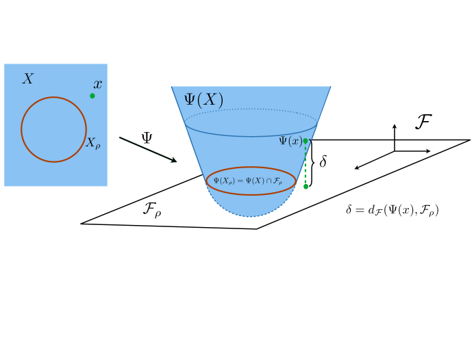
Theorem 1 then implies that Definition 1 and 3 are equivalent. We thus see that the separating property has a clear geometric interpretation in the feature space: the set $\Psi(C)$ is the intersection of the closed subspace $\mathcal{F}_{C}$, i.e. a linear manifold in $\cal F$, and $\Psi(X)$ – see Figure 2.

In the above interpretation, the estimator we propose for the support then stems from the following observation: given a training set $x_{1},\ldots,x_{n}$, we classify a new point $x$ as belonging to the estimator $X_{n}$ of $X_{\rho}$ if the distance of $\Psi(x)$ to the linear span of $\{\Psi(x_{1}),\ldots\Psi(x_{n})\}$ is sufficiently small.

Given a training set $\left\{x_{1},\ldots,x_{n}\right\}$, our estimator $F_{n}$ classifies a new point $x$ as belonging to the support if the distance of $\Psi(x)$ to the linear span of $\Psi(x_{1}),\ldots,\Psi(x_{n})$ is sufficiently small.

Figure 2: The sets $X$ and the support $X_{\rho}$ are mapped into the feature space $\cal F$, by the feature map $\Psi$. Here we take ${\cal F}_{\rho}={\cal F}_{X_{\rho}}$ to be a linear space passing through the origin. The image of the support with respect to the feature map is given by the intersection of the image of $X$ with ${\cal F}_{\rho}$. By the separating property, a point $x$ belongs to the support if and only the distance between $\Psi(x)$ and $\mathcal{F}_{\rho}$ is zero.

6.3 Inverse Problems and Empirical Risk Minimization

Here we suggest a simple interpretation of the estimator $F_{n}$ and stress the connection with the supervised setting. We regard the sampled data $x_{1},\ldots,x_{n}$ as a training set of positive examples, so that each point $x_{i}\in X_{\rho}$ almost surely; the new datum is the point $x\in X$, and we evaluate the estimator $F_{n}$ at $x$. We label the examples according to the similarity function $K$ by setting

$$y_{i}(x)=K(x_{i},x)\equiv({\mathbf{K}}_{x})_{i}\qquad i=1,\ldots,n.$$

If $K$ satisfies Assumption 1, then, since $K(x,x)=1$ and $K$ is $d_{K}$-continuous, the function $y_{i}$ is close to $1$ whenever $x_{i}$ is close to $x$. The interpolation problem

$$\text{find }f\in\mathcal{H}\text{ such that }f(x_{i})=y_{i}(x)\ \forall i\in\{1,\ldots,n\}\quad\Longleftrightarrow\quad S_{n}f={\mathbf{K}}_{x}$$

(where $S_{n}$ is defined in (18)) is ill-posed. To restore well-posedeness we can consider the corresponding least square problem (empirical risk minimization problem)

$$\min_{f\in\mathcal{H}}\frac{1}{n}\sum_{i=1}^{n}\left\lvert{f(x_{i})-y_{i}(x)}\right\rvert^{2}\quad\Longleftrightarrow\quad\min_{f\in\mathcal{H}}\frac{1}{n}\left\lVert{S_{n}f-{\mathbf{K}}_{x}}\right\rVert^{2}_{{\mathbb{R}^{n}}},$$

or in fact its regularized version

$$\min_{f\in\mathcal{H}}\left(\frac{1}{n}\sum_{i=1}^{n}\left\lvert{f(x_{i})-y_{i}(x)}\right\rvert^{2}+\lambda\left\lVert{f}\right\rVert^{2}\right)\quad\Longleftrightarrow\quad\min_{f\in\mathcal{H}}\left(\frac{1}{n}\left\lVert{S_{n}f-{\mathbf{K}}_{x}}\right\rVert^{2}_{{\mathbb{R}^{n}}}+\lambda\left\lVert{f}\right\rVert^{2}\right),$$

where $\lambda>0$ is the regularization parameter (Tikhonov regularization). It is known [34] that the minimum of the above expression is achieved by $f\equiv f_{n}^{\lambda}$, with

$$f_{n}^{\lambda}=\frac{1}{n}g_{\lambda}(\frac{S_{n}^{\top}S_{n}}{n})S^{\top}_{n}y,$$

where $g_{\lambda}$ is the function $g_{\lambda}(\sigma)=1/(\sigma+\lambda)$.
More generally, Tikhonov regularization can be replaced by spectral regularization induced by a different choice of the filter $g_{\lambda}$; the corresponding regularized solution $f_{n}^{\lambda}$ is still given by the previous equation, but the function $g_{\lambda}$ appearing in it is now completely arbitrary. Comparing with (19), we see that $f^{\lambda_{n}}_{n}(x)=F_{n}(x)$. Equation (17) has then the following interpretation: a new point $x$ is estimated to be a positive example (that is, to belong to the support $X_{\rho}$) if and only if $f^{\lambda_{n}}_{n}(x)\geq 1-\tau$, where $\tau$ is a threshold parameter.

The above discussion suggests several extensions and variations of our method, obtained considering more general penalized empirical risk minimization functionals of the form

$$\min_{f\in\mathcal{H}}\left(\frac{1}{n}\sum_{i=1}^{n}V(y_{i}(x),f(x_{i}))+\lambda R(f)\right),$$

where:

• $V$ is a (regression) loss function measuring the approximation property of $f$, for example the logistic loss or a robust loss such as the one used in support vector machine regression. Our theoretical analysis does not carry on to other loss functions and different mathematical concepts from empirical process theory are probably needed;

• $R$ is a regularizer measuring the complexity of a function $f\in\mathcal{H}$. For example, one can consider the case where the kernel is given by a dictionary of atoms $f_{\gamma}:X\to{\mathbb{R}}$, with $\gamma\in\Gamma$, such that $\sum_{\gamma\in\Gamma}\left\lvert{f_{\gamma}(x)}\right\rvert^{2}=1$, so that we have $K(x,y)=\sum_{\gamma\in\Gamma}f_{\gamma}(x){f_{\gamma}(y)}$ and, hence, ${f=\sum_{\gamma\in\Gamma}w_{\gamma}f_{\gamma}}$, with $w=(w_{\gamma})_{\gamma\in\Gamma}\in\ell_{2}(\Gamma)$. In this setting, Tikhonov regularization corresponds to the choice $R(f)=\sum_{\gamma\in\Gamma}\left\lvert{w_{\gamma}}\right\rvert^{2}$, but other norms, such as the $\ell_{1}$ norm $\sum_{\gamma\in\Gamma}|w_{\gamma}|$, can also be considered.

7 Empirical Analysis

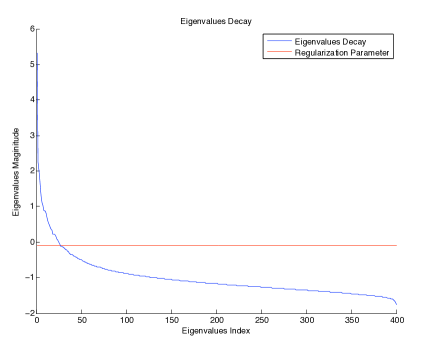
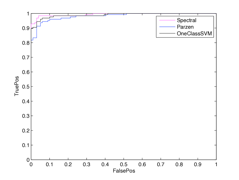
In this section we describe some preliminary experiments aimed at testing the properties and the performances of the proposed methods both on simulated and real data. We only discuss spectral algorithms induced by Tikhonov regularization to contrast the general method to some current state of the art algorithms. Note that while computations can be made more efficient in several ways, we consider a simple algorithmic protocol and leave a more refined computational study for future work. Recall that Tikhonov regularization defines an estimator $F_{n}(x)={\mathbf{K}_{x}}^{\ast}({\mathbf{K}}_{n}+n\lambda)^{-1}{\mathbf{K}}_{x}$, and a point $x$ is labeled as belonging to the support $X_{\rho}$ if $F_{n}(x)\geq 1-\tau$. The computational cost for the algorithm is, in the worst case, of order $n^{3}$ – like standard regularized least squares – for training, and order $Nn^{2}$ if we have to predict the value of $F_{n}$ at $N$ test points. In practice, one has to choose a good value for the regularization parameter $\lambda$ and this requires computing multiple solutions, a so called regularization path. As noted in [57], if we form the inverse using the eigendecomposition of the kernel matrix the price of computing the full regularization path is essentially the same as that of computing a single solution (note that the cost of the eigen-decomposition of ${\mathbf{K}}_{n}$ is also of order $n^{3}$, though the constant is worse). This is the strategy that we consider in the following. In our experiments we considered two datasets: the MNIST dataset and the CBCL face database. For the digits we considered a reduced set consisting of a training set of 5000 images and a test set of 1000 images. In the first experiment we trained on $500$ images for the digit $3$ and tested on $200$ images of digits $3$ and $8$. Each experiment consists of training on one class and testing on two different classes and was repeated for 20 trials over different training set choices. For all our experiments we considered the Abel kernel. Note that in this case the algorithm requires to choose $3$ parameters: the regularization parameter $\lambda$, the kernel width $\sigma$ and the threshold $\tau$. In supervised learning cross validation is typically used for parameter tuning, but cannot be used in our setting since support estimation is an unsupervised problem. Then, we considered the following heuristics. The kernel width is chosen as the median of the distribution of distances of the $k$-th nearest neighbor of each training set point for $k=10$. Fixed the kernel width, we choose the regularization parameter in correspondence of the maximum curvature in the eigenvalue behavior – see Figure 3 – the rationale being that after this value the eigenvalues are relatively small.

Figure 3: Decay of the eigenvalues of the kernel matrix ordered in decreasing magnitude and corresponding regularization parameter in logarithimic scale.

MNIST $9vs4$

MNIST $1vs7$

CBCL

Figure 4: ROC curves for the different estimator in three different tasks: digit $9$vs $4$ (Left), digit $1$vs $7$ (Center), CBCL (Right).

	$3$vs $8$	$8$vs $3$	$1$vs $7$	$9$vs $4$	CBCL
Spectral	$0.837\pm 0.006$	$0.783\pm 0.003$	$0.9921\pm 0.0005$	$0.865\pm 0.002$	$0.868\pm 0.002$
Parzen	$0.784\pm 0.007$	$0.766\pm 0.003$	$0.9811\pm 0.0003$	$0.724\pm 0.003$	$0.878\pm 0.002$
1CSVM	$0.790\pm 0.006$	$0.764\pm 0.003$	$0.9889\pm 0.0002$	$0.753\pm 0.004$	$0.882\pm 0.002$

Table 2: Average and standard deviation of the AUC for the different estimators on the considered tasks.

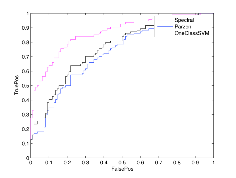
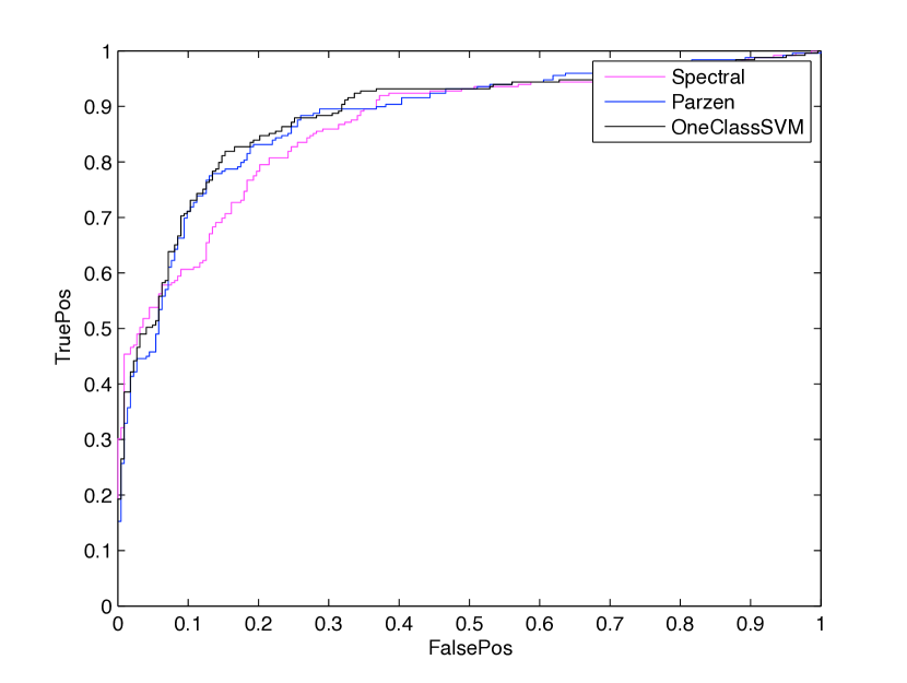
For comparison we considered a Parzen window density estimator and one-class SVM (1CSVM) as implemented by [11]. For the Parzen window estimator we used the same kernel of the spectral algorithm, that is the Laplacian kernel, and also the same width. Given a kernel width, an estimate of the probability distribution is computed and can be used to estimate the support by fixing a threshold $\tau^{\prime}$. For the one-class SVM we considered the Gaussian kernel, so that we have to fix the kernel width and a regularization parameter $\nu$. We fixed the kernel width to be the same used by our estimator and set $\nu=0.9$. For the sake of comparison, also for one-class SVM we considered a varying offset $\tau^{{}^{\prime\prime}}$. The performance is evaluated computing ROC curve (and the corresponding AUC value) for varying values of the thresholds $\tau,\tau^{\prime},\tau^{{}^{\prime\prime}}$. The ROC curves on the different tasks are reported (for one of the trials) in Figure 4, Left. The mean and standard deviation of the AUC for the three methods is reported in Table 2. Similar experiments were repeated considering other pairs of digits, see Table 2. Also in the case of the CBCL datasets we considered a reduced dataset consisting of $472$ images for training and other $472$ for test. On the different test performed on the MNIST data the spectral algorithm always achieves results which are better – and often substantially better – than those of the other methods. On the CBCL dataset SVM provides the best result, but spectral algorithm still provides a competitive performance.

Remark 8.

We remark that, although binary classification data sets are used in the experiments, the considered set-up is that of a one-class classification problem. Indeed, the training and tuning of the algorithms are performed using only examples of one class and the other class is only considered for testing. Accordingly, the proposed methods are compared to state of the art algorithms for one-class classification.

Appendix A Auxiliary Proofs

In this section we give the proofs of a few technical results needed in the paper.

A.1 Normalizing a Kernel

The next result shows that, if $K$ is a reproducing kernel which is nonzero on the diagonal, then it can be normalized, and its normalized version separates the same sets. When $K(x,x)=0$ for some $x\in X$, then clearly this result still holds replacing the set $X$ with $X\setminus X_{0}$ and considering the restriction of $K$ to $(X\setminus X_{0})\times(X\setminus X_{0})$, where $X_{0}=\left\{x\in X\mid K(x,x)=0\right\}$.

Proposition 13.

Assume that $K(x,x)>0$ for all $x\in X$. Then, the reproducing kernel $K^{\prime}$ on $X$, given by

$$K^{\prime}(x,y)=\dfrac{K(x,y)}{\sqrt{K(x,x)K(y,y)}}\qquad\forall x,y\in X,$$

is normalized and separates the same sets as $K$.

Proof.

Clearly $K$ is a kernel of positive type. Denote by $\mathcal{H}^{\prime}$ the reproducing kernel Hilbert space with kernel $K^{\prime}$, and define the feature map $\Psi:X\to\mathcal{H}$, $\Psi(x)=K_{x}/\left\lVert{K_{x}}\right\rVert$. It is simple to check that $\left\langle{\Psi(y)},{\Psi(x)}\right\rangle=K^{\prime}(x,y)$ and $\Psi(X)^{\perp}=\{0\}$, so that the map $\Psi_{*}:\mathcal{H}\to\mathcal{H}^{\prime}$

$$(\Psi_{*}f)(x)=\left\langle{f},{\Psi(x)}\right\rangle$$

is a unitary operator with $K^{\prime}_{x}=\Psi_{*}(\Psi(x))$ [15]. Clearly, for any $f\in\mathcal{H}$ and $x\in X$

$$\left\langle{\Psi_{*}f},{K^{\prime}_{x}}\right\rangle=\left\langle{\Psi_{*}f},{\Psi_{*}\Psi(x)}\right\rangle=\frac{\left\langle{f},{K_{x}}\right\rangle}{\left\lVert{K_{x}}\right\rVert}.$$

The above equality shows that $\mathcal{H}$ and $\mathcal{H}^{\prime}$ separate the same sets. ∎

A.2 Analytic Results

In this section, we suppose that the kernel $K$ satisfies Assumption 1, and endow the set $X$ with the metric $d_{K}$ induced by $K$. Measurability of a map taking values in a topological space will be always understood with respect to the Borel $\sigma$-algebra of such space. The next simple lemma will be used frequently.

Lemma 5.

For all $k=1,2$, the map

$$\xi:X\to\mathcal{S}_{k},\qquad\xi(x)=K_{x}\otimes K_{x}$$

is continuous and measurable. Moreover, if $Z_{i}:\Omega\to\mathcal{S}_{k}$ is given by

$$Z_{i}(\omega)=K_{x_{i}}\otimes K_{x_{i}}\qquad\omega=(x_{j})_{j\geq 1},$$

then $Z_{i}$ is measurable for all $i\geq 1$.

Proof.

The map ${x\mapsto K_{x}}$, is continuous from $X$ into $\mathcal{H}$ by item i) in Proposition 1. Since $\xi(x)=K_{x}\otimes K_{x}$, continuity of $\xi$ follows at once. By item v) in Proposition 1, $\xi$ is then a measurable map, hence $Z_{i}$ is such. ∎

We recall some basic properties of the operator $T$ defined by the kernel. The next result is known (see for example [26]), but we report a short proof for completeness.

Proposition 14.

The $\mathcal{S}_{1}$-valued map $\xi$ defined in Lemma 5 is Bochner-integrable with respect to $\rho$, and its integral

$$T=\int_{X}K_{x}\otimes K_{x}d\rho(x)$$

is a positive trace class operator on $\mathcal{H}$, with $\left\lVert{T}\right\rVert_{\mathcal{S}_{1}}=\operatorname{tr}\left[T\right]=1$.

Proof.

The map $\xi$ isbounded because $\left\lVert{K_{x}\otimes K_{x}}\right\rVert_{\mathcal{S}_{1}}=\operatorname{tr}\left[K_{x}\otimes K_{x}\right]=K(x,x)=1$ and measurable by Lemma 5 . Therefore, $\xi$ is a Bochner-integrable $\mathcal{S}_{1}$-valued map, and its integral $T$ is a trace class operator. As $\xi(x)$ is a positive operator for all $x$, so is $T$. In particular, $\left\lVert{T}\right\rVert_{\mathcal{S}_{1}}=\operatorname{tr}\left[T\right]$, and $\operatorname{tr}\left[T\right]=\int_{X}\operatorname{tr}\left[K_{x}\otimes K_{x}\right]d\rho(x)=1$. ∎

Now, we come to the proof of Proposition 7. We will split it into the proofs of Propositions 15 and 16 below.

Lemma 6.

For all $k=1,2$, the map

$$\check{T}_{n}:X^{n}\to{\mathcal{S}}_{k},\qquad\check{T}_{n}(x_{1},\ldots,x_{n}){=}\frac{1}{n}\sum_{i=1}^{n}K_{x_{i}}\otimes K_{x_{i}}$$

is continuous and measurable.

Proof.

Evident by Lemma 5. ∎

Proposition 15.

For all $n\geq 1$, the map $T_{n}$ defined in (15) is a $\mathcal{S}_{k}$-valued estimator for $k=1,2$.

Proof.

We have

$$T_{n}(\omega)=\check{T}_{n}(x_{1},\ldots,x_{n})\qquad\omega=(x_{i})_{i\geq 1},$$

hence $T_{n}$ is measurable by Lemma 6. ∎

For the next proposition we recall that the topology of uniform convergence on compact subsets of $X$ is generated by the following basis of open sets $U_{f,\epsilon,C}\subset C(X)$

$$U_{f,\epsilon,C}=\left\{g\in C(X)\mid\sup_{x\in C}\left\lvert{f(x)-g(x)}\right\rvert<\epsilon\right\}\qquad f\in C(X),\,\epsilon>0,\,C\subset X\mbox{ compact}.$$

Proposition 16.

Suppose $X$ is locally compact. Let $(r_{\lambda})_{\lambda>0}$ be a family of functions $r_{\lambda}:[0,1]\to[0,1]$ such that each $r_{\lambda}$ is upper semicontinuous. Then, for any sequence of positive numbers $(\lambda_{n})_{n\geq 1}$ and all $n\geq 1$, the map $F_{n}$ defined in (16) is a $C(X)$-valued estimator, where $C(X)$ is the space of continuous functions on $X$ with the topology of uniform convergence on compact subsets.

Proof.

Throughout the proof, $n\geq 1$ will be fixed. Let $(\varphi_{k})_{k\geq 1}$ be a decreasing sequence of continuous functions $\varphi_{k}:[0,1]\to[0,1]$ such that $\varphi_{k}(\sigma)\downarrow r_{\lambda_{n}}(\sigma)$ for all $\sigma\in[0,1]$ (such sequence exists by (12.7.8) of [31]). Then, by Lemma 6 and continuity of the functional calculus (see e.g. Problem 126 in [37]), for all $k\geq 1$ the map

$$\varphi_{k}(\check{T}_{n}):X^{n}\to{\mathcal{S}}_{0},\qquad[\varphi_{k}(\check{T}_{n})](x_{1},\ldots,x_{n}){=}\varphi_{k}(\check{T}_{n}(x_{1},\ldots,x_{n}))$$

is continuos from $X^{n}$ into the Banach space ${\mathcal{S}}_{0}$ of the bounded operators on $\mathcal{H}$ with the uniform operator norm. Thus, for all $x\in X$, the real function $(x_{1},\ldots,x_{n})\mapsto\left\langle{[\varphi_{k}(\check{T}_{n})](x_{1},\ldots,x_{n})\,K_{x}},{K_{x}}\right\rangle$ is continuous on $X^{n}$, hence is measurable by item v) of Proposition 1. By spectral calculus and dominated convergence theorem, for all $\omega=(x_{i})_{i\geq 1}$

$$\left\langle{r_{\lambda_{n}}(T_{n}(\omega))\,K_{x}},{K_{x}}\right\rangle =\left\langle{r_{\lambda_{n}}(\check{T}_{n}(x_{1},\ldots,x_{n}))\,K_{x}},{K_{x}}\right\rangle=\lim_{k\to\infty}\left\langle{[\varphi_{k}(\check{T}_{n})](x_{1},\ldots,x_{n})\,K_{x}},{K_{x}}\right\rangle$$

It then follows that, for each $x\in X$, the real function $\omega\mapsto\left\langle{r_{\lambda_{n}}(T_{n}(\omega))K_{x}},{K_{x}}\right\rangle$ is measurable on $\Omega$, being the pointwise limit of measurable functions.
We now prove that the map $F_{n}:\omega\mapsto(x\mapsto\left\langle{r_{\lambda_{n}}(T_{n}(\omega))K_{x}},{K_{x}}\right\rangle)$ is measurable from $\Omega$ into the space $C(X)$. By M2, p. 115 in [45], this is equivalent to the measurability of the subsets $F_{n}^{-1}(U)\subset\Omega$ for all open sets $U\subset C(X)$. Since $X$ is a locally compact separable metric space, the topology of uniform convergence on compact subsets is a separable metric topology on $C(X)$ by (12.14.6.2) in [31]. By separability of $C(X)$, each open set $U\subset C(X)$ then is the denumerable union of sets of the neighborhood basis $\{U_{f,\epsilon,C}\mid f\in C(X),\,\epsilon>0,\,C\subset X\mbox{ compact}\}$. Hence, it is enough to show that $F_{n}^{-1}(U_{f,\epsilon,C})$ is measurable for all $f$, $\epsilon$ and $C$. We have

$$F_{n}^{-1}(U_{f,\epsilon,C})=\left\{{\omega\in\Omega}\mid\sup_{x\in C}\left\lvert{f(x)-\left\langle{r_{\lambda_{n}}(T_{n}({\omega}))\,K_{x}},{K_{x}}\right\rangle}\right\rvert<\epsilon\right\}.$$

By separability of $X$, there exists a countable set $C_{0}\subset C$ such that $\overline{C_{0}}=C$. A continuity argument then shows that

$$F_{n}^{-1}(U_{f,\epsilon,C}) =\bigcap_{k\geq 1}\left\{{\omega\in\Omega}\mid\sup_{x\in C}\left\lvert{f(x)-\left\langle{r_{\lambda_{n}}(T_{n}({\omega}))\,K_{x}},{K_{x}}\right\rangle}\right\rvert\leq\epsilon-\frac{1}{k}\right\}$$

$$=\bigcap_{k\geq 1}\bigcap_{x\in C_{0}}\left\{{\omega\in\Omega}\mid\left\lvert{f(x)-\left\langle{r_{\lambda_{n}}(T_{n}({\omega}))\,K_{x}},{K_{x}}\right\rangle}\right\rvert\leq\epsilon-\frac{1}{k}\right\}.$$

Since each set $\left\{{\omega\in\Omega}\mid\left\lvert{f(x)-\left\langle{r_{\lambda_{n}}(T_{n}({\omega}))\,K_{x}},{K_{x}}\right\rangle}\right\rvert\leq\epsilon-1/k\right\}$ is measurable in $\Omega$, measurability of the countable intersection $F_{n}^{-1}(U_{f,\epsilon,C})$ then follows. ∎

We conclude this section with the proof of measurability of the threshold parameters $(\tau_{n})_{n\geq 1}$ defined in (30).

Proposition 17.

Suppose $X$ is locally compact. Let $(r_{\lambda})_{\lambda>0}$ be a family of functions $r_{\lambda}:[0,1]\to[0,1]$ such that each $r_{\lambda}$ is upper semicontinuous. Then, for any sequence of positive numbers $(\lambda_{n})_{n\geq 1}$ and all $n\geq 1$, the map $\tau_{n}$ defined in (30) is a $\mathbb{R}$-valued estimator.

Proof.

As $F_{n}$ depends only on $(x_{1},\ldots,x_{n})$, it is clear that so does $\tau_{n}$. It remains to show measurability of $\tau_{n}$.
Given $i\geq 1$, the map $\omega\mapsto x_{i}$ is measurable by definition of the product $\sigma$-algebra $\mathcal{A}_{\Omega}$ on $\Omega$. Moreover, for any $n\geq 1$, the map $F_{n}$ is measurable from $\Omega$ into $C(X)$ by Proposition 16. Therefore, the map $\Theta_{1}:\Omega\to C(X)\times X$, with $\Theta_{1}(\omega)=(F_{n}(\omega)\,,\,x_{i})$, is measurable when $C(X)\times X$ is endowed with the product $\sigma$-algebra of the Borel $\sigma$-algebras of $C(X)$ and $X$, respectively.
Since $X$ is locally compact, the map $\Theta_{2}:C(X)\times X\to\mathbb{R}$, with $\Theta_{2}(f,x)=f(x)$, is jointly continuous by [41, Theorem 5, p. 223] and the discussion following it. Thus, $\Theta_{2}$ is measurable with respect to the Borel $\sigma$-algebras of $C(X)\times X$ and $\mathbb{R}$.
The metric spaces $X$ and $C(X)$ are both separable (for $C(X)$, this is (12.14.6.2) in [31]). By [32, Proposition 4.1.7], the product $\sigma$-algebra of the Borel $\sigma$-algebras of $C(X)$ and $X$ then coincides with the Borel $\sigma$-algebra of $C(X)\times X$. Thus, the composition map $\Phi_{i}=\Theta_{2}\Theta_{1}$, which is $\Phi_{i}(\omega)=[F_{n}(\omega)](x_{i})$, is measurable.
Finally, the map $m(t_{1},\ldots,t_{n})\mapsto\min_{1\leq i\leq n}t_{i}$ is continuous from $\mathbb{R}^{n}$ into $\mathbb{R}$, so that $\tau_{n}=1-m(\Phi_{1},\Phi_{2},\ldots,\Phi_{n})$ is measurable. ∎

A.3 A Useful Inequality

The following proof of inequality (45) below is due to A. Maurer.

Lemma 7.

Suppose $S$ and $T$ are two symmetric Hilbert-Schmidt operators on $\mathcal{H}$ with spectrum contained in the interval $[a,b]$, and let $(\sigma_{j})_{j\in J}$ and $(\tau_{k})_{k\in K}$ be the eigenvalues of $S$ and $T$, respectively. Given a function $r:[a,b]\to\mathbb{R}$, if the constant

$$L=\sup_{j\in J,k\in K}\left\lvert{\frac{r(\sigma_{j})-r(\tau_{k})}{\sigma_{j}-\tau_{k}}}\right\rvert\qquad(\mbox{with }0/0\equiv 0)$$

is finite, then

$$\left\lVert{r(S)-r(T)}\right\rVert_{\mathcal{S}_{2}}\leq L\left\lVert{S-T}\right\rVert_{\mathcal{S}_{2}}.$$ (44)

In particular, if $r$ is a Lipshitz function with Lipshitz constant $L_{r}$, then

$$\left\lVert{r(S)-r(T)}\right\rVert_{\mathcal{S}_{2}}\leq L_{r}\left\lVert{S-T}\right\rVert_{\mathcal{S}_{2}}.$$ (45)

Proof.

Let $(f_{j})_{j\in J}$ and $(g_{k})_{k\in K}$ be the orthonormal bases of eigenvectors of $S$ and $T$ corresponding to the eigenvalues $(\sigma_{j})_{j\in J}$ and $(\tau_{k})_{k\in K}$, respectively, which here we list repeated accordingly to their multiplicity. We have

$$\left\lVert{r(S)-r(T)}\right\rVert_{\mathcal{S}_{2}}^{2} =\sum_{j,k}\left\lvert{\left\langle{(r(S)-r(T))f_{j}},{g_{k}}\right\rangle}\right\rvert^{2}=\sum_{j,k}\left(r(\sigma_{j})-r(\tau_{k})\right)^{2}\left\lvert{\left\langle{f_{j}},{g_{k}}\right\rangle}\right\rvert^{2}$$

$$\leq L^{2}\sum_{j,k}\left(\sigma_{j}-\tau_{k}\right)^{2}\left\lvert{\left\langle{f_{j}},{g_{k}}\right\rangle}\right\rvert^{2}=L^{2}\sum_{j,k}\left\lvert{\left\langle{(S-T)f_{j}},{g_{k}}\right\rangle}\right\rvert^{2}$$

$$=L^{2}\left\lVert{S-T}\right\rVert_{\mathcal{S}_{2}}^{2},$$

which is (44). ∎

A.4 Concentration of Measure Results

We will use the following standard concentration inequality for Hilbert space random variables (see Theorem 8.6 in [53], and [54]). Let $\mathcal{V}$ be a separable Hilbert space and $(\Omega,\mathcal{A}_{\Omega},{\mathbb{P}})$ a probability space. Suppose that $Y_{1},Y_{2},\ldots$ is a sequence of independent $\mathcal{V}$-valued random variables $Y_{i}:\Omega\to\mathcal{V}$. If ${\mathbb{E}}[\left\lVert{Y_{i}}\right\rVert_{\mathcal{V}}^{m}]\leq(1/2)m!B^{2}L^{m-2}$ $\forall m\geq 2$, then, for all $n\geq 1$ and $\epsilon>0$,

$${\mathbb{P}}\left(\left\lVert{\frac{1}{n}\sum_{i=1}^{n}Y_{i}}\right\rVert_{\mathcal{V}}>\epsilon\right)\leq 2e^{-\frac{n\epsilon^{2}}{B^{2}+L\epsilon+B\sqrt{B^{2}+2L\epsilon}}}.$$ (46)

We will need in particular the next two straightforward consequences of this inequality.

Lemma 8.

If $Z_{1},Z_{2},\ldots$ is a sequence of i.i.d. $\mathcal{V}$-valued random variables, such that $\left\lVert{Z_{i}}\right\rVert_{\mathcal{V}}\leq M$ almost surely, ${\mathbb{E}}[Z_{i}]=\mu$ and ${\mathbb{E}}[\left\lVert{Z_{i}}\right\rVert_{\mathcal{V}}^{2}]\leq\sigma^{2}$ for all $i$, then, for all $n\geq 1$ and $\delta>0$,

$$\left\lVert{\frac{1}{n}\sum_{i=1}^{n}Z_{i}-\mu}\right\rVert_{\mathcal{V}}\leq\frac{M\delta}{n}+\sqrt{\frac{2\sigma^{2}\delta}{n}}$$ (47)

with probability at least $1-2e^{-\delta}$.

Proof.

Let $Y_{i}=Z_{i}-\mu$. Then $\left\lVert{Y_{i}}\right\rVert_{\mathcal{V}}\leq 2M$ and ${\mathbb{E}}[\left\lVert{Y_{i}}\right\rVert_{\mathcal{V}}^{2}]\leq{\mathbb{E}}[\left\lVert{Z_{i}}\right\rVert_{\mathcal{V}}^{2}]=\sigma^{2}$. Moreover, for all $i$ and $m\geq 2$ ${\mathbb{E}}[\left\lVert{Y_{i}}\right\rVert_{\mathcal{V}}^{m}]\leq\sigma^{2}(2M)^{m-2}\leq(1/2)m!\sigma^{2}M^{m-2}$, where the last inequality follows since $2^{m-2}\leq m!/2$. Then,

$${\mathbb{P}}\left(\left\lVert{\frac{1}{n}\sum_{i=1}^{n}Z_{i}-\mu}\right\rVert_{\mathcal{V}}>\epsilon\right)={\mathbb{P}}\left(\left\lVert{\frac{1}{n}\sum_{i=1}^{n}Y_{i}}\right\rVert_{\mathcal{V}}>\epsilon\right)\leq 2e^{-\frac{n\epsilon^{2}}{\sigma^{2}+M\epsilon+\sigma\sqrt{\sigma^{2}+2M\epsilon}}}=2e^{-\frac{\sigma^{2}n}{M^{2}}g(\frac{M\epsilon}{\sigma^{2}})}=2e^{-\delta},$$

where $g(t)=t^{2}/(1+t+\sqrt{1+2t})$.
Since $g^{-1}(t)=t+\sqrt{2t}$, by solving the equation $(\sigma^{2}n/M^{2})g(M\epsilon/\sigma^{2})=\delta$ we have

$$\epsilon=\frac{\sigma^{2}}{M}\left(\frac{M^{2}\delta}{n\sigma^{2}}+\sqrt{\frac{2M^{2}\delta}{n\sigma^{2}}}\right)=\frac{M\delta}{n}+\sqrt{\frac{2\sigma^{2}\delta}{n}}.$$

∎

The above result and Borel-Cantelli lemma imply that

$$\lim_{n\to\infty}\left\lVert{\frac{1}{n}\sum_{i=1}^{n}Z_{i}-\mu}\right\rVert_{\mathcal{V}}=0$$

almost surely. In the paper we actually need a slightly stronger result which is given in the following lemma.

Lemma 9.

If $Z_{1},Z_{2},\ldots$ is a sequence of i.i.d. $\mathcal{V}$-valued random variables, such that $\left\lVert{Z_{i}}\right\rVert_{\mathcal{V}}\leq M$ almost surely, then we have

$$\lim_{n\to\infty}\frac{\sqrt{n}}{\log n}\left\lVert{\frac{1}{n}\sum_{i=1}^{n}Z_{i}-\mu}\right\rVert_{\mathcal{V}}=0$$

almost surely.

Proof.

We continue with the notations in the proof of Lemma 8. By (46), for all $\epsilon>0$ we have

$${\mathbb{P}}\left(\frac{\sqrt{n}}{\log n}\left\lVert{\frac{1}{n}\sum_{i=1}^{n}Z_{i}-\mu}\right\rVert_{\mathcal{V}}>\epsilon\right)={\mathbb{P}}\left(\left\lVert{\frac{1}{n}\sum_{i=1}^{n}Y_{i}}\right\rVert_{\mathcal{V}}>\epsilon\,\frac{\log n}{\sqrt{n}}\right)\leq 2e^{-A(n,\epsilon)}=2\left(\frac{1}{n}\right)^{\frac{A(n,\epsilon)}{\log n}},$$

with

$$A(n,\epsilon){=}\frac{\epsilon^{2}\log^{2}n}{\sigma^{2}+M\epsilon\frac{\log n}{\sqrt{n}}+\sigma\sqrt{\sigma^{2}+2M\epsilon\frac{\log n}{\sqrt{n}}}}.$$

It follows that

$$\sum_{n\geq 1}{\mathbb{P}}\left(\frac{\sqrt{n}}{\log n}\left\lVert{\frac{1}{n}\sum_{i=1}^{n}Z_{i}-\mu}\right\rVert_{\mathcal{V}}>\epsilon\right)\leq 2\,\sum_{n\geq 1}\left(\frac{1}{n}\right)^{\frac{A(n,\epsilon)}{\log n}}.$$

For all $\epsilon>0$, $\lim_{n\to\infty}A(n,\epsilon)/\log n=+\infty$, so that the series $\sum_{n\geq 1}n^{-A(n,\epsilon)/\log n}$ is convergent, and Borel-Cantelli lemma gives the result. ∎

The following inequality is given in [13] and we report its proof for completeness.

Lemma 10.

If Assumption 1 holds true, then for all $\delta>0$ we have

$$\left\lVert{(T+\lambda)^{-1}(T-T_{n})}\right\rVert_{\mathcal{S}_{2}}\leq\left(\frac{\delta}{n\lambda}+\sqrt{\frac{2\delta{\cal N}(\lambda)}{n\lambda}}\right)$$

with probability at least $1-2e^{-\delta}$.

Proof.

Let $(\Omega,\mathcal{A}_{\Omega},{\mathbb{P}})$ be the probability space defined at the beginning of Section 5.1. For all $i\geq 1$ we define the random variable $Y_{i}:\Omega\to\mathcal{S}_{2}$ as

$$Y_{i}(\omega)=(T+\lambda)^{-1}(K_{x_{i}}\otimes K_{x_{i}})\qquad\omega=(x_{j})_{j\geq 1},$$

which is measurable by Lemma 5. Then, we have $\left\lVert{Y_{i}}\right\rVert_{\mathcal{S}_{2}}\leq 1/\lambda$ almost surely, ${\mathbb{E}}[Y_{i}]=(T+\lambda)^{-1}T$, $(1/n)\sum_{i=1}^{n}Y_{i}=(T+\lambda)^{-1}T_{n}$ and

$${\mathbb{E}}[\left\lVert{Y_{i}}\right\rVert^{2}_{\mathcal{S}_{2}}] =\int_{\Omega}\operatorname{tr}\left[Y_{i}(\omega)^{\ast}Y_{i}(\omega)\right]d{\mathbb{P}}\left(\omega\right)=\int_{X}\operatorname{tr}\left[(T+\lambda)^{-2}(K_{x}\otimes K_{x})\right]d\rho(x)$$

$$=\operatorname{tr}\left[(T+\lambda)^{-2}T\right]\leq\left\lVert{(T+\lambda)^{-1}}\right\rVert_{\infty}\operatorname{tr}\left[(T+\lambda)^{-1}T\right]\leq\frac{{\cal N}(\lambda)}{\lambda},$$

where we have bounded the operator norm $\left\lVert{(T+\lambda)^{-1}}\right\rVert_{\infty}$ by $1/\lambda$. The result follows applying Lemma 8. ∎

References

- [1] W. K. Allard, G. Chen, and M. Maggioni. Multiscale Geometric Methods for Data Sets II: Geometric Multi-Resolution Analysis. Appl. Comput. Harmon. A. 32 (2012) 435–462..
- [2] N. Aronszajn. Theory of reproducing kernels. T. Am. Math. Soc. 68 (1950) 337–404.
- [3] F. Bauer, S. Pereverzev, and L. Rosasco. On regularization algorithms in learning theory. J. Complexity 23 (2007) 52–72.
- [4] M. Belkin and P. Niyogi. Laplacian eigenmaps for dimensionality reduction and data representation. Neural Comput. 15 (2003) 1373–1396.
- [5] M. Belkin, P. Niyogi and V. Sindhwani Manifold Regularization: A Geometric Framework for Learning from Labeled and Unlabeled Examples. J. Mach. Learn. Res. 7 (2006) 2399–2434
- [6] M. Belkin and P. Niyogi. Towards a theoretical foundation for Laplacian-based manifold methods. J. Comput. Syst. Sci. 74 (2008) 1289–1308.
- [7] C. Berg, J. Christensen, and P. Ressel. Harmonic analysis on semigroups. Springer-Verlag, New York, 1984.
- [8] G. Biau, B. Cadre, D. Mason, and B. Pelletier. Asymptotic normality in density support estimation. Electron. J. Probab. 14 (2009) 2617–2635.
- [9] M. Birman and M. Solomyak. Double operator integrals in a Hilbert space. Integr. Equat. Oper. Th. 47 (2003) 131–168.
- [10] O. Bousquet, S. Boucheron, and G. Lugosi. Theory of classification: A survey of recent advances. ESAIM Probab. Stat. 9 (2004) 323–375.
- [11] S. Canu, Y. Grandvalet, V. Guigue, and A. Rakotomamonjy. SVM and kernel methods matlab toolbox. Perception Systèmes et Information, INSA de Rouen, Rouen, France, 2005.
- [12] A. Caponnetto. Optimal Rates for Regularization Operators in Learning Theory. Technical report, MIT (CSAIL), Cambridge, MA, 2006.
- [13] A. Caponnetto and E. De Vito. Optimal rates for the regularized least-squares algorithm. Found. Comput. Math. 7 (2007) 331–368.
- [14] A. Caponnetto and Y. Yao. Cross-validation based adaptation for regularization operators in learning theory. Anal. Appl. 8 (2010) 161–183.
- [15] C. Carmeli, E. De Vito, and A. Toigo. Vector valued reproducing kernel Hilbert spaces of integrable functions and Mercer theorem. Anal. Appl. 4 (2006) 377–408.
- [16] C. Carmeli, E. De Vito, A. Toigo, and V. Umanità. Vector valued reproducing kernel hilbert spaces and universality. Anal. Appl. 8 (2010) 19–61.
- [17] V. Chandola, A. Banerjee, and V. Kumar. Anomaly detection: A survey. ACM Comput. Surv. 41 (2009) 1–58.
- [18] G. Chen, A. Little, M. Maggioni, and L. Rosasco. Some recent advances in multiscale geometric analysis of point clouds, in: Wavelets and multiscale analysis, Birkhäuser/Springer, New York, 2011, pp. 199–225.
- [19] R. Coifman and S. Lafon. Geometric harmonics: a novel tool for multiscale out-of-sample extension of empirical functions. Appl. Comput. Harmon. A. 21 (2006) 31–52.
- [20] R. Coifman, S. Lafon, A. Lee, M. Maggioni, B. Nadler, S. Warner, and S. Zucker. Geometric diffusions as a tool for harmonic analysis and structure definition of data: diffusion maps. P. Natl. Acad. Sci. USA 102 (2005) 7426–7431.
- [21] R. Coifman, S. Lafon, A. Lee, M. Maggioni, B. Nadler, S. Warner, and S. Zucker. Geometric diffusions as a tool for harmonic analysis and structure definition of data: multiscale methods. P. Natl. Acad. Sci. USA 102 (2005) 7432–7438.
- [22] F. Cucker and S. Smale. On the mathematical foundations of learning. B. Am. Math. Soc. 39 (2002) 1–49.
- [23] A. Cuevas and R. Fraiman. A plug-in approach to support estimation. Ann. Stat. 25 (1997) 2300–2312.
- [24] A. Cuevas and R. Fraiman. Set estimation, in: New perspectives in stochastic geometry, Oxford Univ. Press, Oxford, 2010, pp. 374–397.
- [25] A. Cuevas and A. Rodríguez-Casal. Set estimation: an overview and some recent developments, in: Recent advances and trends in nonparametric statistics, Elsevier B. V., Amsterdam, 2003, pp. 251–264.
- [26] C. De Mol, E. De Vito, and L. Rosasco. Elastic-net regularization in learning theory. J. Complexity 25 (2009) 201–230.
- [27] V. De Silva J. B. Tenenbaum, and J. C. Langford. A global geometric framework for nonlinear dimensionality reduction. Science 290 (2000) 2319–2323.
- [28] E. De Vito, L. Rosasco, and A. Toigo. Spectral regularization for support estimation, in: Advances in Neural Information Processing Systems 24, MIT Press, Cambridge, MA, 2010, pp. 487–495.
- [29] L. Devroye, L. Györfi, and G. Lugosi. A Probabilistic Theory of Pattern Recognition. Springer, New York, 1996.
- [30] L. Devroye and G. L. Wise. Detection of abnormal behavior via nonparametric estimation of the support. SIAM J. Appl. Math. 38 (1980) 480–488.
- [31] J. Dieudonné. Treatise on analysis. Vol. II. Academic Press, New York, San Francisco and London, 1976.
- [32] R. M. Dudley. Real Analysis and Probability. Cambridge University Press, Cambridge, 2002.
- [33] L. Dümbgen and G. Walther. Rates of convergence for random approximations of convex sets. Adv. Appl. Probab. 28 (1996) 384–393.
- [34] H. W. Engl, M. Hanke, and A. Neubauer. Regularization of inverse problems. Kluwer Academic Publishers Group, Dordrecht, 1996.
- [35] G. Folland. A course in abstract harmonic analysis. CRC Press, Boca Raton, FL, 1995.
- [36] L. Györfi, M. Kohler, A. Krzyzak, and H. Walk. A distribution-free theory of nonparametric regression. Springer-Verlag, New York, Berlin, Paris, 2002.
- [37] P. Halmos. A Hilbert space problem book. Springer-Verlag, New York, 1982.
- [38] T. Hastie, R. Tibshirani, and J. Friedman. The Elements of Statistical Learning. Springer, New York, 2001.
- [39] H. Hoffmann. Kernel PCA for novelty detection. Pattern Recogn. 40 (2007) 863–874.
- [40] M. Kazhdan, M. Bolitho, and H. Hoppe. Poisson surface reconstruction, in: Proceedings of the fourth Eurographics symposium on Geometry processing, Eurographics Association, Aire-la-Ville, 2006, pp. 61–70.
- [41] J. L. Kelley. General topology. Reprint of the 1955 edition [Van Nostrand, Toronto, Ont.]. Graduate Texts in Mathematics, No. 27. Springer-Verlag, New York-Berlin, 1975.
- [42] R. Kolluri, J. Shewchuk, and J. O’Brien. Spectral surface reconstruction from noisy point clouds, in: Proceedings of the 2004 Eurographics/ACM SIGGRAPH symposium on Geometry processing, ACM, New York, 2004, pp. 11–21.
- [43] V. Koltchinskii. Oracle inequalities in empirical risk minimization and sparse recovery problems. Springer, Heidelberg, 2011.
- [44] A. P. Korostelëv and A. B. Tsybakov. Minimax theory of image reconstruction. Springer-Verlag, New York, 1993.
- [45] S. Lang. Real and functional analysis. Springer-Verlag, New York, 1993.
- [46] G. Lerman and T. Zhang. Probabilistic recovery of multiple subspaces in point clouds by geometric minimization. arXiv:1002.1994v2, 2010.
- [47] D. Levin. Mesh-independent surface interpolation, in: Geometric Modeling for Scientific Visualization, Springer-Verlag, 2003, pp. 37–49.
- [48] L. Lo Gerfo, L. Rosasco, F. Odone, E. De Vito, and A. Verri. Spectral algorithms for supervised learning. Neural Comput. 20 (2008) 1873–1897.
- [49] A. Maurer and M. Pontil. -dimensional coding schemes in hilbert spaces. IEEE T. Inform. Theory 56 (2010) 5839–5846.
- [50] J. Mercer. Functions of positive and negative type and their connection with the theory of integral equations. Phil. Trans. R. Soc. A 209 (1909) 415–446.
- [51] H. Narayanan and S. Mitter. Sample complexity of testing the manifold hypothesis, in: Advances in Neural Information Processing Systems 24, MIT Press, Cambridge, MA, 2010, pp. 1786–1794.
- [52] P. Niyogi, S. Smale, and S. Weinberger. A topological view of unsupervised learning from noisy data. SIAM J. Comput. 40 (2011) 646–663.
- [53] I. Pinelis. Optimum bounds for the distributions of martingales in Banach spaces. Ann. Probab. 22 (1994) 1679–1706.
- [54] I. Pinelis. Correction: optimum bounds for the distributions of martingales in Banach spaces. Ann. Probab. 27 (1999) 2119.
- [55] T. Poggio and S. Smale. The mathematics of learning: dealing with data. Not. Am. Math. Soc. 50 (2003) 537–544.
- [56] M. Reitzner. Random polytopes and the Efron-Stein jackknife inequality. Ann. Probab. 31 (2003) 2136–2166.
- [57] R. Rifkin and R. Lippert. Notes on regularized least squares. Technical report, Massachusetts Institute of Technology, MIT (CSAIL), Cambridge, MA, 2007.
- [58] L. Rosasco, M. Belkin, and E. De Vito. On learning with integral operators. J. Mach. Learn. Res. 11 (2010) 905–934.
- [59] S. T. Roweis and L.K. Saul. Nonlinear dimensionality reduction by locally linear embedding. Science 290 (2000) 2323–2326.
- [60] B. Schölkopf, J. Giesen, and S. Spalinger. Kernel methods for implicit surface modeling, in: Advances in Neural Information Processing Systems 17, MIT Press, Cambridge, MA, 2005, pp. 1193–1200.
- [61] B. Schölkopf, J. Platt, J. Shawe-Taylor, A. Smola, and R. Williamson. Estimating the support of a high-dimensional distribution. Neural Comput. 13 (2001) 1443–1471.
- [62] B. Schölkopf, A. Smola, and K.-R. Müller. Nonlinear component analysis as a kernel eigenvalue problem. Neural Comput. 10 (1998) 1299–1319.
- [63] C. D. Scott and R. D. Nowak. Learning minimum volume sets. J. Mach. Learn. Res. 7 (2006) 665–704.
- [64] B. Simon. Trace ideals and their applications. Cambridge University Press, Cambridge, 1979.
- [65] S. Smale and D. X. Zhou. Geometry of probability spaces. Constr. Approx. 30 (2009) 311–323.
- [66] E. M. Stein and G. Weiss. Introduction to Fourier analysis on Euclidean spaces. Princeton University Press, Princeton, N. J., 1971.
- [67] I. Steinwart. On the influence of the kernel on the consistency of support vector machines. J. Mach. Learn. Res. 2 (2002) 67–93.
- [68] I. Steinwart and A. Christmann. Support vector machines. Springer, New York, 2008.
- [69] I. Steinwart, D. Hush, and C. Scovel. A classification framework for anomaly detection. J. Mach. Learn. Res. 6 (2005) 211–232.
- [70] I. Steinwart and C. Scovel. Mercer’s theorem on general domains: on the interaction between measures, kernels, and RKHSs. Constr. Approx. 35 (2012) 363–417.
- [71] V. Y. Tikhonov and A. N. Arsenin. Solutions of Ill-Posed Problems. Winston, New York, 1977.
- [72] A. B. Tsybakov. On nonparametric estimation of density level sets. Ann. Stat. 25 (1997) 948–969.
- [73] A. van der Vaart and J. Wellner. Weak convergence and empirical processes. Springer-Verlag, New York, 1996.
- [74] V. N. Vapnik. Statistical learning theory. John Wiley & Sons Inc., New York, 1998.
- [75] R. Vert and J.-P. Vert. Consistency and convergence rates of one-class SVMs and related algorithms. J. Mach. Learn. Res. 7 (2006) 817–854.
- [76] R. Vidal, Y. Ma, and S. Shankar. Generalized principal component analysis (GPCA). IEEE T. Pattern Anal. 27 (2005) 1945–1959.
- [77] L. Zwald and G. Blanchard. On the convergence of eigenspaces in kernel principal component analysis, in: Advances in Neural Information Processing Systems 18, MIT Press, Cambridge, MA, 2006, pp. 1649–1656.