Probability distributions for quantum stress tensors in four dimensions

Abstract

We treat the probability distributions for quadratic quantum fields, averaged with a Lorentzian test function, in four-dimensional Minkowski vacuum. These distributions share some properties with previous results in two-dimensional spacetime. Specifically, there is a lower bound at a finite negative value, but no upper bound. Thus arbitrarily large positive energy density fluctuations are possible. We are not able to give closed form expressions for the probability distribution, but rather use calculations of a finite number of moments to estimate the lower bounds, the asymptotic forms for large positive argument, and possible fits to the intermediate region. The first 65 moments are used for these purposes. All of our results are subject to the caveat that these distributions are not uniquely determined by the moments. However, we also give bounds on the cumulative distribution function that are valid for any distribution fitting these moments. We apply the asymptotic form of the electromagnetic energy density distribution to estimate the nucleation rates of black holes and of Boltzmann brains.

I Introduction

There has been extensive work in recent decades on the definition and use of the expectation value of a quantum stress tensor operator. When this expectation value is used as the source in the Einstein equations, the resulting semiclassical theory gives an approximate description of the effects of quantum matter fields upon the gravitational field. This theory gives, for example, a plausible description of the backreaction of Hawking radiation on black hole spacetimes BD .

However, the semiclassical theory does not describe the effects of quantum fluctuations of the stress tensor around its expectation value. Quantum stress tensor fluctuations and the resulting passive fluctuations of gravity have been the subject of several papers in recent years  WF01 ; Borgman ; Stochastic ; FW04 ; TF06 ; PRV09 ; FW07 ; CG97 ; WKF07 ; FMNWW10 ; WHFN11 ; LN05 ; Wu2007 . However, most of these papers deal with effects described by the correlation function of a pair of stress tensor operators, and ignore higher-order correlation functions.

One way to include these higher-order correlations is through the probability distribution of a smeared stress tensor operator. This distribution was given recently for Gaussian averaged conformal stress tensors in two-dimensional flat spacetime FFR10 . This result will be discussed further in Sec. II.2. A recent attempt to define probability distributions for quantum stress tensors in four dimensions was made by Duplancic, et al Duplancic . However, these authors attempt to define distributions for stress tensor operators at a single spacetime point. Because such operators do not have well-defined moments, the resulting probability distribution is not well-defined. In our view, only temporal or spacetime averages of quantum stress tensors have meaningful probability distributions in four dimensions. Furthermore, these averages should be normal ordered, resulting in a zero mean for the vacuum probability distribution and a nonzero probability of finding negative values. None of these conditions are satisfied by the distribution proposed in Ref. Duplancic .

The purpose of the present paper is to obtain information about the form of the probability distribution for averaged stress tensors in four-dimensional spacetime from calculations of a finite set of moments. This method was used in Ref. FFR10 to infer the distribution for $\varphi^{2}$, with Lorentzian averaging, where $\varphi$ is a massless scalar field four-dimensional Minkowski spacetime. The result matches a shifted Gamma distribution to extremely high numerical accuracy. Unfortunately, the probability distribution of the smeared energy density for massless scalar and electromagnetic fields cannot be found so precisely. However, under certain assumptions to be detailed later, we are able to give approximate lower bounds and asymptotic tails for these cases, and to give a rough fit to the intermediate part of the distribution.

An important point arises here. Throughout this paper, all quadratic operators are understood to be normal-ordered with respect to the Minkowski vacuum state. However, the smeared normal ordered operators are defined, in the first instance, only as symmetric operators on a dense domain in the Hilbert space (assuming a real-valued smearing function) and it is possible that there is more than one way of extending them to provide self-adjoint operators The operators of greatest interest to us are bounded from below on account of quantum inequalities (see Sect. II.1) and so there is a distinguished Friedrichs extension (see Ref. RSii , Theorem X.23), whose lower bound coincides with the sharpest possible quantum inequality bound. It is this operator that we have in mind when we discuss the probability distribution of individual measurements of the smeared operator in the vacuum state. The question of whether there is more than one self-adjoint extension, i.e., whether the normal ordered expressions fail to be essentially self-adjoint, is nontrivial and not fully resolved. Recent results (not, however, immediately applicable to our situation) and references may be found in Ref. Sanders . If there are distinct self-adjoint extensions, their corresponding probability distributions will all share the same moments in the vacuum state.

This links to the wider issue of whether or not the moments of the probability distribution determine the distribution uniquely. There is a rich theory concerning this question, which is reviewed in Ref. Simon . As will be discussed below, some of the moments we study grow too fast to be covered by well-known sufficient criteria (due to Hamburger and Stieltjes) for uniqueness. This does not prove that the distribution is nonunique (nor would the existence of distinct self-adjoint extensions prove nonuniqueness) and we have not been able to resolve the question of uniqueness. However, in Sect. VI we prove that any probability distribution with the moments we find has a cumulative distribution function close to that corresponding to the fitted asymptotic tail. As various applications (see Ref. CMP11 and Sect. VII) depend only on the rough form of the tail, the possible lack of uniqueness is not as crucial as might be thought. Further discussion of this point can be found in Sect. VIII.1.

II Review of Some Previous Results

Here we will briefly summarize selected aspects of two topics, quantum inequality bounds on expectation values, and known results for probability distributions. Both of these related topics are important for the present paper.

II.1 Quantum Inequalities

Quantum inequalities are lower bounds on the smeared expectation values of quantum stress tensor components in arbitrary quantum states F78 ; F91 ; FR95 ; FR97 ; Flanagan97 ; FewsterEveson98 ; Fe&Ho05 . In two-dimensional spacetime, the sampling may be over either space, time, or both. In four dimensions, there must be a sampling either over time alone, or over both space and time, as there are no lower bounds on purely spatially sampled operators FHR02 . Here we will be concerned with sampling in time alone, in which case a quantum inequality takes the form

$$\int_{-\infty}^{\infty}f(t)\,\langle T(t,0)\rangle\,dt\geq-\frac{C}{\tau^{d}}\,,$$ (1)

where $T$ is a normal-ordered quadratic operator, which is classically non-negative, and $f(t)$ is a sampling function with characteristic width $\tau$. Here $C$ is a numerical constant, typically small compared to unity, and $d$ is the number of spacetime dimensions.

Although quantum field theory allows negative expectation values of the energy density, quantum inequalities place strong constraints on the effects of this negative energy for violating the second law of thermodynamics F78 , maintaining traversable wormholes FR96 or warpdrive spacetimes PF97 . The implication of Eq. (1) is that there is an inverse power relation between the magnitude and duration of negative energy density.

For a massless scalar field in two-dimensional spacetime, Flanagan Flanagan97 has found a formula for the constant $C$ for a given $f(t)$ which makes Eq. (1) an optimal inequality, and has constructed the quantum state in which the bound is saturated. This formula is

$$C=\frac{1}{6\pi}\,\int^{\infty}_{-\infty}du\left(\frac{d}{du}\sqrt{g(u)}\right)^{2}\,,$$ (2)

where $f(t)=\tau^{-1}g(u)$ and $u=t/\tau$. This is the $c=1$ special case of a general result for unitary, positive energy, conformal field theories in two dimensions, where $c$ is the central charge, in which the left-hand side of (2) is multiplied by $c$ Fe&Ho05 . In four-dimensional spacetime, Fewster and Eveson FewsterEveson98 have derived an analogous formula for $C$, but in this case the bound is not necessarily optimal.

II.2 Shifted Gamma Distributions

Here we briefly recall the main results of Ref. FFR10 . First, we determined the probability distribution for individual measurements, in the vacuum state, of the Gaussian sampled energy density

$$\rho=\frac{1}{\sqrt{\pi}\,\tau}\int_{-\infty}^{\infty}T_{tt}(t,0)\,{\rm e}^{-t^{2}/\tau^{2}}\,dt$$ (3)

of a general conformal field theory in two-dimensions. This was achieved by finding a closed form expression for the generating function of the moments $\langle\rho^{n}\rangle$ of $\rho$, from which the probability distribution was obtained by inverting a Laplace transform. The resulting distribution is conveniently expressed in terms of the dimensionless variable $x=\rho\,\tau^{2}$ and is a shifted Gamma distribution:

$$P(x)=\vartheta(x+x_{0})\frac{\beta^{\alpha}(x+x_{0})^{\alpha-1}}{\Gamma(\alpha)}\exp(-\beta(x+x_{0}))\,,$$ (4)

with parameters

$$x_{0}=\frac{c}{12\pi},\qquad\alpha=\frac{c}{12},\qquad\beta=\pi\,.$$ (5)

Here $x=-x_{0}$ is the infimum of the support of the probability distribution, which we will often call the lower bound of the distribution, and $c>0$ is the central charge, which is equal to unity for the massless scalar field. Using the binomial theorem and standard integrals, the $n$’th moment

$$a_{n}=\int x^{n}\,P(x)\,dx\,,$$ (6)

of $P$ is easily found to be

$$a_{n}=\frac{x_{0}^{n}}{\Gamma(\alpha)}\sum_{k=0}^{n}\frac{(-1)^{n-k}}{(\beta x_{0})^{k}}\binom{n}{k}\Gamma(k+\alpha)=(-x_{0})^{n}\,\,{}_{2}{F}{{}_{0}}(\alpha,-n;(\beta x_{0})^{-1}),$$ (7)

where ${}_{2}{F}{{}_{0}}$ is a generalized hypergeometric function.

The lower bound, $-x_{0}$, for the probability distribution for energy density fluctuations in the vacuum for $c=1$ is exactly Flanagan’s optimum lower bound, Eq. (2), on the Gaussian sampled expectation value and, for all $c>0$, coincides with the result of Ref. Fe&Ho05 . As was argued in Ref. FFR10 , this is a general feature, giving a deep connection between quantum inequality bounds and stress tensor probability distributions. The quantum inequality bound is the lowest eigenvalue of the sampled operator, and is hence the lowest possible expectation value and the smallest result which can be found in a measurement. That the probability distribution for vacuum fluctuations actually extends down to this value is more subtle and depends upon special properties of the vacuum state. In essence, the Reeh-Schlieder theorem implies a nonzero overlap between the vacuum and the generalized eigenstate of the sampled operator with the lowest eigenvalue.

There is no upper bound on the support of $P(x)$, as arbitrarily large values of the energy density can arise in vacuum fluctuations. Nonetheless, for the massless scalar field, negative values are much more likely; 84% of the time, a measurement of the Gaussian averaged energy density will produce a negative value. However, the positive values found the remaining 16% of the time will typically be much larger, and the average [first moment of $P(x)$] will be zero.

The asymptotic positive tail of $P(x)$ has recently been used by Carlip et al CMP11 to draw conclusions about the small scale structure of spacetime in a two-dimensional model. These authors argue that large positive energy density fluctuations tend to focus light rays on small scales, and cause spacetime to break into many causally disconnected domains at scales somewhat above the Planck length.

In Ref. FFR10 , we also reported on calculations of the moments of ${:}\varphi^{2}{:}$ averaged with a Lorentzian, where $\varphi$ is a massless scalar field in four-dimensional spacetime. It appears that the probability distribution is also a shifted gamma function in this case. Define a dimensionless variable $x$ by

$$x=(4\pi\tau)^{2}\int_{-\infty}^{\infty}f(t)\,\varphi^{2}\,dt\,,$$ (8)

where

$$f(t)=\frac{\tau}{\pi(t^{2}+\tau^{2})}\,.$$ (9)

There is good evidence that the probability distribution is to be Eq. (4) with the parameters

$$\alpha=\frac{1}{72},\qquad\beta=\frac{1}{12},\qquad x_{0}=\frac{1}{6}\,.$$ (10)

These parameters were determined empirically by fitting to the first three calculated moments. However, the resulting distribution matches the first sixty-five moments exactly (agreement had been checked up to the twentieth moment at the time of writing of Ref. FFR10 ), so there can little doubt that it is correct. The details of this calculation are given in Sect. III and Appendix A.

Furthermore, the probability distribution for both the two-dimensional stress tensor and the four-dimensional ${:}\varphi^{2}{:}$ is uniquely determined by its moments, as a consequence of the Hamburger moment theorem Simon . This states that if $a_{n}$ is the $n$-th moment of a probability distribution $P(x)$, then there is no other probability distribution with the same moments provided there exist constants $C$ and $D$ such that

$$|a_{n}|\leq CD^{n}\,n!$$ (11)

for all $n$. This condition is a sufficient, although not necessary, condition for uniqueness, and is fulfilled by the moments of the shifted Gamma distribution. The Hamburger moment theorem is also an existence result: given a real sequence $\{a_{n}\}$, $n=0,1,2,\cdots$ with $a_{0}=1$, such that the $N\times N$-matrix $H^{(N)}_{mn}=a_{m+n}$ ($0\leq m,n\leq N-1$) is strictly positive definite for every $N=1,2,\ldots$, then there exists at least one associated probability distribution for which the $a_{n}$ are the moments.

III Moments and Moment Generating Functions

III.1 Explicit Calculation of Moments

In this section, we describe how the moments of a quadratic quantum operator may be calculated explicitly. Let $\phi$ be a free quantum field or a derivative of a free field, and let $T$ be the smeared normal ordered square of $\phi$:

$$T=\int{:}\phi^{2}{:}(x)\,f(x)\,dx\,,$$ (12)

where $f$ is a sampling function. In our detailed calculations, the smearing will be in time only, and $f=f(t)$ will be the Lorentzian function of Eq. (9), but our preliminary discussion can be more general. The $n$-th moment $\mu_{n}$ of $T$ is formed by smearing the vacuum expectation value

$$G_{n}(x_{1},\ldots,x_{n})=\langle{:}\phi^{2}{:}(x_{1})\cdots{:}\phi^{2}{:}(x_{n})\rangle$$ (13)

over $n$ copies of $f$. By Wick’s theorem, this quantity is equal to the sum of all contractions of the form

$$\contraction{}{\phi(x_{1})}{\phi(x_{1})}{\phi(x_{2})}\bcontraction{\phi(x_{1})}{\phi(x_{1})}{\phi(x_{2})\phi(x_{2})}{\phi(x_{3})}\contraction{\phi(x_{1})\phi(x_{1})\phi(x_{2})}{\phi(x_{2})}{\phi(x_{3})\phi(x_{3})\cdots\phi(x_{n})}{\phi(x_{n})}\bcontraction{\phi(x_{1})\phi(x_{1})\phi(x_{2})\phi(x_{2})\phi(x_{3})}{\phi(x_{3})}{\cdots}{\phi(x_{n})}\phi(x_{1})\phi(x_{1})\phi(x_{2})\phi(x_{2})\phi(x_{3})\phi(x_{3})\cdots\phi(x_{n})\phi(x_{n})\,.$$ (14)

The contractions are subject to the rules that no $\phi(x_{i})$ is contracted with the other copy of itself and all fields are contracted, with each contraction

$$\contraction{}{\phi(x_{i})}{\cdots}{\phi(x_{j})}\phi(x_{i})\cdots\phi(x_{j})$$ (15)

contributing a factor $\langle\phi(x_{i})\phi(x_{j})\rangle$.

It is convenient to represent the contractions by graphs with $n$ vertices labelled $x_{1},\ldots,x_{n}$ placed in order from left to right so that (1) every vertex is met by exactly two lines; (2) every line is directed, pointing to the right; (3) no vertex is connected to itself by a line. For each graph every line from $x_{i}$ to $x_{j}$ contributes the factor $\langle\phi(x_{i})\phi(x_{j})\rangle$ and we supply a combinatorial factor that gives the number of contractions represented by a given graph; we then sum over all distinct graphs of the above type to obtain $G_{n}(x_{1},\ldots,x_{n})$. For example, the graph in Fig. 1a describes the two contractions which contribute to the second moment

$$\mu_{2}=2\int dx_{1}\,dx_{2}f(x_{1})f(x_{2})\langle\phi(x_{1})\phi(x_{2})\rangle^{2}\,,$$ (16)

so the combinatorial factor for $n=2$ is $2$, while Fig. 1b corresponds to the eight contractions pairing a $\phi(x_{1})$ with a $\phi(x_{2})$, a $\phi(x_{1})$ with a $\phi(x_{3})$ and a $\phi(x_{2})$ with a $\phi(x_{3})$, e.g.,

$$\contraction{\phi(x_{1})}{\phi(x_{1})}{}{\phi(x_{2})}\contraction{\phi(x_{1})\phi(x_{1})\phi(x_{2})}{\phi(x_{2})}{\phi(x_{3})}{\phi(x_{3})}\bcontraction{}{\phi(x_{1})}{\phi(x_{1})\phi(x_{2})\phi(x_{2})}{\phi(x_{3})}\phi(x_{1})\phi(x_{1})\phi(x_{2})\phi(x_{2})\phi(x_{3})\phi(x_{3})$$ (17)

and

$$\contraction{}{\phi(x_{1})}{\phi(x_{1})}{\phi(x_{2})}\contraction{\phi(x_{1})\phi(x_{1})\phi(x_{2})}{\phi(x_{2})}{}{\phi(x_{3})}\bcontraction{\phi(x_{1})}{\phi(x_{1})}{\phi(x_{2})\phi(x_{2})\phi(x_{3})}{\phi(x_{3})}\phi(x_{1})\phi(x_{1})\phi(x_{2})\phi(x_{2})\phi(x_{3})\phi(x_{3})\,.$$ (18)

Figure 1: The graphs for $n=2$ (a), and $n=3$ (b) are illustrated.

Note that the moments $\mu_{n}$ have dimensions of inverse powers of length, which depend upon the specific choice of $\phi$. It is convenient to rescale the $\mu_{n}$ and define dimensionless moments $a_{n}$. Our explicit calculations of moments assume the Lorentzian sampling function of width $\tau$ given in Eq. (9). In the case that $\phi=\varphi$, the massless scalar field in four dimensions, we take

$$a_{n}=(4\pi\tau)^{2n}\,\mu_{n}\,.$$ (19)

For the case that $\phi=\dot{\varphi}$, we take

$$a_{n}=(4\pi\tau^{2})^{2n}\,\mu_{n}\,.$$ (20)

We also take the latter form for the cases of the squared electric field, and scalar and electromagnetic field energy densities.

III.2 Moment Generating Functions

For $n\geq 4$, the Wick expansion involves both connected and disconnected graphs. However, we need not consider the disconnected graphs explicitly, as the moment generating function $M$ is the exponential of $W$, the generating function for the connected graphs. The full moment generating function is defined by

$$M(\lambda)=\sum_{n=0}^{\infty}\frac{\lambda^{n}\;a_{n}}{n!}\,,$$ (21)

so the $n$-th moment has the expression

$$a_{n}=\left(\frac{d^{n}M}{d\lambda^{n}}\right)_{\lambda=0}\,.$$ (22)

The connected moment generating function, $W$, has an analogous definition, but in terms of the dimensionless connected moments $C_{n}$ only. These are the moments which arise from counting only connected graphs. For $n=2$, there is a single connected graph, with combinatorial factor $1$ as already described. For $n>2$, there are $\frac{1}{2}(n-1)!$ distinct connected graphs, each with a combinatorial factor $2^{n}$ . Of course, the enumeration of these graphs becomes rapidly unmanageable, and one must exploit further degeneracies among the graphs to reduce the counting. For sampling using the Lorentzian function, it is possible to reduce the number of terms to the number of distinct partitions of $n$ into an even number of terms. This grows much more slowly than $\frac{1}{2}(n-1)!$: for example, for $n=30$, we require $2811$ terms instead of $29!/2\approx 4.4\times 10^{30}$. Further details can be found in Appendix A

Our procedure will be to explicitly compute a finite number $N$ of connected moments, which allows $W$ to be approximated as an $N$-th degree polynomial in $\lambda$. We then use

$$M={\rm e}^{W}$$ (23)

to find $M$, which may also be approximated as an $N$-th degree polynomial. Finally, the first $N$ moments $a_{n}$ may be read off from the coefficients of this polynomial. We emphasize that this procedure makes sense whether or not the series (21) converges; expressions such as (23) are simply convenient expressions for the combinatorial relation between different moments and may be understood as formal power series.

Consider the case of $\varphi^{2}$ in four dimensions, where $\varphi$ is a massless scalar field and the average is in the time direction only. The two-point function which appears in the integrals for the moments is now

$$\langle\phi(t)\phi(t^{\prime})\rangle=\langle\varphi(t)\varphi(t^{\prime})\rangle=-\frac{1}{4\pi^{2}(t-t^{\prime}-i\epsilon)^{2}}=\frac{1}{4\pi^{2}}\int_{0}^{\infty}d\alpha\,\alpha{\rm e}^{-i\alpha(t-t^{\prime}-i\epsilon)}\,.$$ (24)

The corresponding dimensionless moments were calculated using MAPLE for $N\leq 65$, and the resulting moments up to $N=23$ are listed in the first column of Table 1. Our computations were exact and give the $a_{n}$ as rational numbers. However, for ease of display, the results have been rounded to five significant figures. The full set of exact moments is available as Supplementary Material SM . As stated earlier, these moments may be used to infer that the probability distribution of the quantity in (8) is a shifted gamma given by Eqs. (4) and (10). Only the first three moments are needed for this fit, but the result reproduces the first 65 moments exactly, a spectacular agreement.

Next we turn to the case where $\phi=\dot{\varphi}$ and calculate several of the moments of the Lorentz-smearing of $\dot{\varphi}^{2}$. In this case we use

$$\langle\phi(t)\phi(t^{\prime})\rangle=\langle\dot{\varphi}(t)\dot{\varphi}(t^{\prime})\rangle=\frac{3}{2\pi^{2}(t-t^{\prime}-i\epsilon)^{4}}=\frac{1}{4\pi^{2}}\int_{0}^{\infty}d\alpha\,\alpha^{3}e^{-i\alpha(t-t^{\prime}-i\epsilon)}\,.$$ (25)

As before, the moments were computed exactly as rational numbers using MAPLE for $N\leq 65$ SM , and the resulting moments up to $N=23$ are listed in the second column of Table 1.

Table 1: Lorentzian smearings of the Wick square of the free massless field $\varphi^{2}$, the Wick square of its time derivative $\dot{\varphi}^{2}$, the square of the electric field strength $E^{2}$, and the energy densities of the scalar and electromagnetic fields $\rho_{S}$ and $\rho_{EM}$ respectively.

$n$	$\varphi^{2}$	$\dot{\varphi}^{2}$	$E^{2}$	$\rho_{S}$	$\rho_{EM}$
0	1	1	1	1	1
1	0	0	0	0	0
2	2	9/2	6	3/2	3
3	48	1890	1680	525/2	420
4	1740	$2.5516\times 10^{6}$	$1.5121\times 10^{6}$	$1.6538\times 10^{5}$	$1.8903\times 10^{5}$
5	83904	$8.5527\times 10^{9}$	$3.3789\times 10^{9}$	$2.7057\times 10^{8}$	$2.1119\times 10^{8}$
6	$5.0516\times 10^{6}$	$6.0498\times 10^{13}$	$1.5934\times 10^{13}$	$9.4918\times 10^{11}$	$4.9794\times 10^{11}$
7	$3.6472\times 10^{8}$	$7.9890\times 10^{17}$	$1.4027\times 10^{17}$	$6.2499\times 10^{15}$	$2.1918\times 10^{15}$
8	$3.0708\times 10^{10}$	$1.7862\times 10^{22}$	$2.0908\times 10^{21}$	$6.9804\times 10^{19}$	$1.6334\times 10^{19}$
9	$2.9538\times 10^{12}$	$6.2613\times 10^{26}$	$4.8861\times 10^{25}$	$1.2231\times 10^{24}$	$1.9086\times 10^{23}$
10	$3.1956\times 10^{14}$	$3.2427\times 10^{31}$	$1.6870\times 10^{30}$	$3.1669\times 10^{28}$	$3.2949\times 10^{27}$
11	$3.8406\times 10^{16}$	$2.3696\times 10^{36}$	$8.2184\times 10^{34}$	$1.1570\times 10^{33}$	$8.0257\times 10^{31}$
12	$5.0767\times 10^{18}$	$2.3561\times 10^{41}$	$5.4477\times 10^{39}$	$5.7522\times 10^{37}$	$2.6600\times 10^{36}$
13	$7.3196\times 10^{20}$	$3.0960\times 10^{46}$	$4.7723\times 10^{44}$	$3.7793\times 10^{42}$	$1.1651\times 10^{41}$
14	$1.1432\times 10^{23}$	$5.2487\times 10^{51}$	$5.3938\times 10^{49}$	$3.2036\times 10^{47}$	$6.5843\times 10^{45}$
15	$1.9226\times 10^{25}$	$1.1252\times 10^{57}$	$7.7085\times 10^{54}$	$3.4338\times 10^{52}$	$4.7049\times 10^{50}$
16	$3.4641\times 10^{27}$	$2.9981\times 10^{62}$	$1.3693\times 10^{60}$	$4.5748\times 10^{57}$	$4.1789\times 10^{55}$
17	$6.6572\times 10^{29}$	$9.7841\times 10^{67}$	$2.9791\times 10^{65}$	$7.4647\times 10^{62}$	$4.5458\times 10^{60}$
18	$1.3592\times 10^{32}$	$3.8605\times 10^{73}$	$7.8364\times 10^{70}$	$1.4726\times 10^{68}$	$5.9787\times 10^{65}$
19	$2.9384\times 10^{34}$	$1.8209\times 10^{79}$	$2.4642\times 10^{76}$	$3.4730\times 10^{73}$	$9.4000\times 10^{70}$
20	$6.7046\times 10^{36}$	$1.0164\times 10^{85}$	$9.1702\times 10^{81}$	$9.6935\times 10^{78}$	$1.7491\times 10^{76}$
21	$1.6103\times 10^{39}$	$6.6549\times 10^{90}$	$4.0026\times 10^{87}$	$3.1733\times 10^{84}$	$3.8172\times 10^{81}$
22	$4.0607\times 10^{41}$	$5.0695\times 10^{96}$	$2.0327\times 10^{93}$	$1.2087\times 10^{90}$	$9.6927\times 10^{86}$
23	$1.0727\times 10^{44}$	$4.4604\times 10^{102}$	$1.1923\times 10^{99}$	$5.3172\times 10^{95}$	$2.8427\times 10^{92}$

Once we have a finite set of moments for $\dot{\varphi}^{2}$, we can calculate the corresponding moments for several other operators of physical interest: we give the examples of the energy densities for the massless scalar and electromagnetic fields, and the squares of the electric and magnetic field strengths as particular examples. These all take the form

$$A=\int_{-\infty}^{\infty}dtf(t)\sum_{I}\alpha_{I}{:}\phi_{I}^{2}{:}(t,0)\,,$$ (26)

where $\alpha_{I}$ are constants and the $\phi_{I}$ are (components of) free fields [in the sense that the Wick expansion is valid] with two point functions obeying

$$c_{I}\delta_{IJ}\langle\dot{\varphi}(t,\mathbf{x})\dot{\varphi}(t^{\prime},\mathbf{x^{\prime}})\rangle_{\mathbf{x}=\mathbf{x^{\prime}}=0}$$ (27)

in the vacuum state, where $\varphi$ is the massless free scalar field as before and the $c_{I}$ are constants. Defining the dimensionless moments for $A$ in the same way as for $\dot{\varphi}^{2}$, one easily sees that the contribution of any connected diagram becomes a sum over $I$ of the contributions from each species $\phi_{I}$, with no cross terms mixing different species in any given term. Thus

$$C_{n}(A)=\sum_{I}(\alpha_{I}c_{I})^{n}C_{n}(\dot{\varphi}^{2})\,,$$ (28)

from which we may infer

$$W(A,\lambda)=\sum_{n=0}^{\infty}\frac{\lambda^{n}\,C_{n}(A)}{n!}=\sum_{I}W(\dot{\varphi}^{2},\alpha_{I}c_{I}\lambda)$$ (29)

and

$$M(A,\lambda)=e^{W(A,\lambda)}=\prod_{I}M(\dot{\varphi}^{2},\alpha_{I}c_{I}\lambda)\,.$$ (30)

These results hold for arbitrary smearing on the time axis.

This procedure may be applied to the energy density operator for the massless scalar field

$$\rho_{S}=\frac{1}{2}\left(\dot{\varphi}^{2}+\partial_{i}\varphi\,\partial^{i}\varphi\right)\,,$$ (31)

because

$$\langle\dot{\varphi}(t)\partial^{i}\varphi(t^{\prime})\rangle_{\mathbf{x}=\mathbf{x^{\prime}}=0} =0$$ (32)

$$\langle\partial_{i}\varphi(t)\partial_{j}\varphi(t^{\prime})\rangle_{\mathbf{x}=\mathbf{x^{\prime}}=0} =\frac{1}{3}\,\delta_{ij}\,\langle\dot{\varphi}(t)\dot{\varphi}(t^{\prime})\rangle_{\mathbf{x}=\mathbf{x^{\prime}}=0}\,,$$ (33)

which is seen by direct computation of the left-hand side and comparison with Eq. (25). Thus we find

$$C_{n}(\rho_{S})=\left(\frac{1}{2^{n}}+\frac{3}{6^{n}}\right)C_{n}(\dot{\varphi}^{2})\,;$$ (34)

the factor of $3$ appearing in one of the numerators corresponds to the spatial dimension. Thus

$$W(\rho_{S},\lambda) =W\left(\dot{\varphi}^{2},\frac{1}{2}\lambda\right)+3W\left(\dot{\varphi}^{2},\frac{1}{6}\lambda\right)$$ (35)

and

$$M(\rho_{S},\lambda) =M(\dot{\varphi}^{2},\frac{1}{2}\lambda)\;\left[M\left(\dot{\varphi}^{2},\frac{1}{6}\lambda\right)\right]^{3}\,.$$ (36)

Again, these results should be understood as a relation between formal power series. Concretely, given the first $N$ moments of $\dot{\varphi}^{2}$, we can approximate $M(\dot{\varphi}^{2},\lambda)$ as a polynomial, and then use the above relation to find the first $N$ moments of $\rho_{S}$. The results are tabulated in the fourth column of Table 1.

Similarly, the components of the square of the electric and magnetic field strength $E_{i}$ and $B_{i}$ obey

$$\langle E_{i}(t)\,E_{j}(t^{\prime})\rangle_{\mathbf{x}=\mathbf{x^{\prime}}=0}=\langle B_{i}(t)\,B_{j}(t^{\prime})\rangle_{\mathbf{x}=\mathbf{x^{\prime}}=0}=\frac{2}{3}\,\delta_{ij}\,\langle\dot{\varphi}(t)\dot{\varphi}(t^{\prime})\rangle_{\mathbf{x}=\mathbf{x^{\prime}}=0}\,.$$ (37)

Following the same line of reasoning as before, we find

$$C_{n}(E^{2})=C_{n}(B^{2})=3\left(\frac{2}{3}\right)^{n}\,C_{n}(\dot{\varphi}^{2})\,,$$ (38)

$$W(E^{2},\lambda)=W(B^{2},\lambda)=3W\left(\dot{\varphi}^{2},\frac{2}{3}\lambda\right)\,,$$ (39)

and

$$M(E^{2},\lambda)=M(B^{2},\lambda)=\left[M\left(\dot{\varphi}^{2},\frac{2}{3}\lambda\right)\right]^{3}\,.$$ (40)

This result leads to the moments of the squared electric field, tabulated in the third column in Table 1. The results for the square of the magnetic field are identical.

Finally, because we also have

$$\langle E_{i}(t,\mathbf{x})B_{j}(t^{\prime},\mathbf{x^{\prime}})\rangle_{\mathbf{x}=\mathbf{x^{\prime}}=0}=0\,,$$ (41)

the energy density of the electromagnetic field

$$\rho_{EM}=\frac{1}{2}\left(E^{2}+B^{2}\right)$$ (42)

has connected moments

$$C_{n}(\rho_{EM})=2\left(\frac{1}{2}\right)^{n}\,C_{n}(E^{2})=6\left(\frac{1}{3}\right)^{n}\,C_{n}(\dot{\varphi}^{2})\,,$$ (43)

and hence

$$W(\rho_{EM},\lambda)=2W\left(E^{2},\frac{1}{2}\lambda\right)=6W\left(\dot{\varphi}^{2},\frac{1}{3}\lambda\right)\,,$$ (44)

and

$$M(\rho_{EM},\lambda)=\left[M\left(E^{2},\frac{1}{2}\lambda\right)\right]^{2}=\left[M\left(\dot{\varphi}^{2},\frac{1}{3}\lambda\right)\right]^{6}\,,$$ (45)

leading to the remaining entries in Table 1.

An important observation is that these moments (apart from those of the Wick square) grow too rapidly to satisfy the Hamburger moment criterion, Eq. (11). This may be confirmed by noting that in all cases $\ln\,a_{n}$ grows faster with increasing $n$ than $n\,\ln n+c_{1}n+c_{0}$ for any constants $c_{0}$ and $c_{1}$. In fact, the growth for $\dot{\varphi}^{2}$ is shown in Appendix B to be of the form

$$a_{n}\sim C\,D^{n}\,(3n-4)!\,,$$ (46)

where the constant $D$ is proved to lie in the range $3.221667<D<3.616898$ (our numerical evidence suggests $D\sim 3.3586$). For probability distributions known to be confined to a half-line, which is the case here, there is a sufficient condition for uniqueness which is weaker than the Hamburger moment criterion. This is the Stieltjes criterion Simon , which is

$$a_{n}\leq C\,D^{n}\,(2n)!\,.$$ (47)

Unfortunately, this criterion is also not fulfilled here. This means that we cannot be guaranteed of finding a unique probability distribution $P(x)$ from these moments. This issue will be discussed further in Sec. VIII.1.

Note that in four dimensions, the operators $(\dot{\varphi}^{2}$, $E^{2}$, $\rho_{S}$, and $\rho_{EM})$ all have dimensions of $length^{-4}$. Their probability distributions $P(x)$ will be taken to be functions of the dimensionless variable [See Eq. (20).]

$$x=(4\pi\,\tau^{2})^{2}\,A\,,$$ (48)

where $A$ is the Lorentzian time average of $(\dot{\varphi}^{2}$, $E^{2}$, $\rho_{S}$, $\rho_{EM})$.

III.3 Lower Bounds

In general, we may use relations between different moment generating functions to find relations between the corresponding probability distributions, and especially between the lower bounds of these distributions. (Strictly, these are the infima of the support of the distributions.) Let $p(x)$ and $q(x)$ be two probability distributions, with moment generating functions $M(p,\lambda)$ and $M(q,\lambda)$, respectively. These generating functions can be expressed in terms of the bilateral Laplace transforms of their probability distributions:

$$M(p,\lambda)=\int_{-\infty}^{\infty}p(x)\,{\rm e}^{\lambda x}\,dx$$ (49)

and

$$M(q,\lambda)=\int_{-\infty}^{\infty}q(x)\,{\rm e}^{\lambda x}\,dx\,.$$ (50)

These integrals are guaranteed to converge at the lower limits, due to the lower bounds on the support of our probability distributions. To assure convergence at the upper limit, we may assume ${\rm Re}\,\lambda<0$. However, many of our arguments below do not require convergence of the integrals, which may be regarded as formal power series in $\lambda$ on replacing the exponential by its Taylor series. Now let $p*q(x)$ be a probability distribution defined as the convolution of $p$ and $q$:

$$p*q(x)=\int_{-\infty}^{\infty}dx^{\prime}\,p(x-x^{\prime})\,q(x^{\prime})\,.$$ (51)

As is well-known in probability theory, this is the distribution for the random variable obtained as the sum of independent random variables with distributions $p$ and $q$, and its moment generating function is

$$M(p*q,\lambda) = \int_{-\infty}^{\infty}dx\,\int_{-\infty}^{\infty}dx^{\prime}\,p(x-x^{\prime})\,q(x^{\prime})\,{\rm e}^{\lambda x}$$ (52)

$$= \int_{-\infty}^{\infty}dx^{\prime}\,\left[\int_{-\infty}^{\infty}dx\,p(x-x^{\prime})\,{\rm e}^{\lambda(x-x^{\prime})}\right]q(x^{\prime})\,{\rm e}^{\lambda x^{\prime}}$$

$$= \left[\int_{-\infty}^{\infty}du\,p(u)\,{\rm e}^{\lambda u}\right]\;\left[\int_{-\infty}^{\infty}dx^{\prime}\,q(x^{\prime})\,{\rm e}^{\lambda x^{\prime}}\right]\ =M(p,\lambda)\;M(q,\lambda)\,,$$

where $u=x-x^{\prime}$ . Thus the moment generating function of a convolution is the product of the individual generating functions; again, this holds in the sense of formal power series, irrespective of convergence issues.

We can also give the relation of the lower bounds. As is also well-known in probability theory, the support of a convolution $p*q$ of two distributions consists of all values expressible as the sum of a value in the support of $p$ and a value in the support of $q$. In particular, the greatest lower bound on the support is the sum of the lower bounds of the individual distributions. Explicitly, if $b_{p}$ and $b_{q}$ be the lower bounds of $p$ and $q$, then

$$p(x)=0\quad{\rm if}\quad x<b_{p}\;;\qquad q(x)=0\quad{\rm if}\quad x<b_{q}\,.$$ (53)

The integrand of Eq. (51) vanishes if either $x^{\prime}<b_{q}$, or $x-x^{\prime}<b_{p}$. This implies that

$$p*q(x)=0\quad{\rm if}\quad x<b_{p}+b_{q}\,,$$ (54)

and in fact this is the greatest lower bound. Thus the lower bound of $p*q$ is the sum of the bounds of $p$ and of $q$.

Next consider the effect of a rescaling of $\lambda$, and let $p_{\alpha}(x)=|\alpha|\,p(\alpha\,x)$, where $\alpha\neq 0$. Then

$$M(p_{\alpha},\lambda)=|\alpha|\int_{-\infty}^{\infty}p(\alpha x)\,{\rm e}^{\lambda x}\,dx=\int_{-\infty}^{\infty}p(x^{\prime})\,{\rm e}^{(\lambda/\alpha)x^{\prime}}\,dx^{\prime}=M\left(p,\frac{\lambda}{\alpha}\right)\,.$$ (55)

Provided $\alpha>0$, $p_{\alpha}=0$ if $x<b_{p}/\alpha$, so the effect of rescaling $\lambda$ in $M$ is a rescaling of the lower bound by the same factor. If $\alpha<0$, the lower bound on the support of $p_{\alpha}$ is $-|\alpha|^{-1}$ times the upper bound on the support of $p$, if this exists; if there is no upper bound on the support of $p$, then evidently $p_{\alpha}$ has no lower bound in this case.

Now we may combine these results to relate the lower bounds of various probability distributions to that for $\dot{\varphi}^{2}$. Applied to a general operator of the form (26), they suggest that the probability distribution for $A$ is a convolution of several copies of the probability distribution for $\dot{\varphi}^{2}$, with various scalings. For example, Eq. (36) suggests that the probability distribution for the energy density $\rho_{S}$, smeared along the time axis, is equal to the convolution of four copies of the probability distribution for $\dot{\varphi}^{2}$, with various scalings. In particular, recalling that $x_{0}(A)$ denotes the greatest lower bound on the support of the distribution for $A$ smeared in time, this suggests that

$$x_{0}(A)=\left(\sum_{I}\alpha_{I}c_{I}\right)x_{0}(\dot{\varphi}^{2})$$ (56)

Hence Eq. (36) suggests that $x_{0}(\rho_{S})=(1/2+3\times\,1/6)x_{0}(\dot{\varphi}^{2})=x_{0}(\dot{\varphi}^{2})$. Similarly, Eq. (40) suggests that $x_{0}(E^{2})=3\times\,(2/3)x_{0}(\dot{\varphi}^{2})=2\,x_{0}(\dot{\varphi}^{2})$, and Eq. (45) suggests that $x_{0}(\rho_{EM})=2\times\,(1/2)x_{0}(E^{2})=x_{0}(E^{2})$. In summary,

$$x_{0}(\rho_{EM})=x_{0}(E^{2})=2\,x_{0}(\rho_{S})=2\,x_{0}(\dot{\varphi}^{2})\,.$$ (57)

Likewise, if we consider a combination such as the pressure $T_{11}=\frac{1}{2}(\dot{\varphi}^{2}+(\partial_{1}\varphi)^{2}-(\partial_{2}\varphi)^{2}-(\partial_{3}\varphi)^{2})$, we obtain the expected result that the probability distribution is unbounded both from above and below. The above derivations should be take as suggestive, rather than rigorous proofs, because of concerns about the uniqueness of the underlying probability distributions. However, it would be possible to prove them by writing the smeared operator for $\rho_{S}$, for example, as a sum of mutually commuting self-adjoint operators, each of which was essentially a multiple of the smeared $\dot{\varphi}^{2}$ operator (under a suitable unitary transformation). This could be done by writing the field in a basis of spherical harmonics, in this framework, the three powers of $M(\dot{\varphi}^{2},\lambda/6)$ arise from the $\ell=1$ angular momentum sector, while the single power of $M(\dot{\varphi}^{2},\lambda/2)$ arises from the $\ell=0$ sector. Indeed, one of the first quantum inequality bounds on the expectation value of $\rho_{S}$ used precisely this decomposition FR95 . More generally, Eq. (27) could be used in conjunction with Wick’s theorem to show that timelike smearings of ${:}\phi_{I}^{2}{:}$ and ${:}\phi_{J}^{2}{:}$ commute for $I\neq J$, at least in matrix elements between states obtained from the vacuum by applying polynomials of smeared fields, and might be used to put the other relationships above on a firmer footing; we will not pursue this here.

IV Lower Bound Estimates

Here we will discuss a technique, a Stieltjes moment test, by which knowledge of a finite number of moments may be used to obtain an approximate estimate of the lower bound. If $P(x)$ is a probability distribution with a lower bound at $x=-x_{0}$, then its moments are

$$a_{n}=\int_{-x_{0}}^{\infty}x^{n}\,P(x)\,dx\,.$$ (58)

Let

$$I(y)=\int_{-x_{0}}^{\infty}(x+y)\,|q(x)|^{2}P(x)\,dx\,,$$ (59)

where $q(x)$ is a polynomial and $y\geq x_{0}$. We see that $I(y)\geq 0$ because the integrand in Eq. (59) is non-negative. If

$$q(x)=\sum_{n=0}^{N-1}\beta_{n}\,x^{n}\,,$$ (60)

then

$$I(y)=\sum_{m,n=0}^{N-1}M_{mn}(N,y)\beta_{m}^{*}\beta_{n}\geq 0\,,$$ (61)

where $M(N,y)$ is a real symmetric $N\times N$ matrix with elements

$$M_{mn}(N,y)=a_{m+n+1}+ya_{m+n}\qquad(0\leq m,n\leq N-1)\,.$$ (62)

Let $\beta_{n}$ be the components of an eigenvector with eigenvalue $\lambda$, then $\sum_{n=0}^{N-1}M_{mn}(N,y)\,\beta_{n}=\lambda\,\beta_{m}$, and $I(y)=\lambda\,\sum_{m=0}^{N-1}|\beta_{m}|^{2}$. It follows that $M(N,y)$ has no negative eigenvalues, that is, it is a positive semidefinite matrix, which we denote by $M(N,y)\geq 0$. This holds for all $N$ and all $y\geq x_{0}$. However, as $y$ decreases below $x_{0}$, the lowest eigenvalue is eventually zero and then negative eigenvalues can occur. Define $y_{N}$ as the minimum value of $y$ at which $M(N,y)\geq 0$; in practice, it is easiest to compute $y_{N}$ as the largest root of the $N$’th degree polynomial equation

$${\rm det}M(N,y)=0\,.$$ (63)

Because $M(N,y)$ is a leading principal minor of $M(N+1,y)$, $M(N+1,y)\geq 0$ implies that $M(N,y)\geq 0$. Consequently, $y_{N+1}\geq y_{N}$ and the sequence in $N$ converges to a limit with

$$y_{\infty}=\lim_{N\rightarrow\infty}y_{N}\leq x_{0}\,.$$ (64)

Given a set of moments $a_{n}$ of an unknown probability distribution, we may form the matrices $M(N,y)$ as above and determine the values of $y_{N}$. The above argument shows that if $y_{N}\to\infty$ then the $a_{n}$ cannot be the moments of a probability distribution whose support is bounded from below. On the other hand, suppose that a finite limit $y_{\infty}$ exists. Then for any probability distribution $\tilde{P}$ with the same moments and support bounded below by $-\tilde{x}_{0}$, we have $y_{\infty}\leq\tilde{x}_{0}$. In particular, there is no probability distribution accounting for the given moments with support contained in $(-y_{\infty},\infty)$.

Table 2: Table of the lower bounds, $y_{N}$, for both $\varphi^{2}$ and $\dot{\varphi}^{2}$.

$N$	$y_{N}(\varphi^{2})$	$y_{N}(\dot{\varphi}^{2})$
2	0.08304597359	0.01071401240
3	0.11085528820	0.01414254029
4	0.12478398360	0.01584995314
5	0.13314891433	0.01690199565
6	0.13872875370	0.01762865715
7	0.14271593142	0.01816742316
8	0.14570717836	0.01858660399
9	0.14803421582	0.01892432539
10	0.14989616852	0.01920370321
11	0.15141979779	0.01943965011
12	0.15268963564	0.01964226267

$N$	$y_{N}(\varphi^{2})$	$y_{N}(\dot{\varphi}^{2})$
13	0.15376421805	0.01981864633
14	0.15468536476	0.01997396248
15	0.15548374872	0.02011206075
16	0.15618237796	0.02023587746
17	0.15679884907	0.02034769569
18	0.15734684979	0.02044932047
19	0.15783718730	0.02054219985
20	0.15827850807	0.02062751059
21	0.15867781217	0.02070622001
22	0.15904082736	0.02077913144
23	0.15937228553	0.02084691828

$N$	$y_{N}(\varphi^{2})$	$y_{N}(\dot{\varphi}^{2})$
24	0.15967613018	0.02091014970
25	0.15995567400	0.02096931050
26	0.16021372020	0.02102481644
27	0.16045265677	0.02107702642
28	0.16067453067	0.02112625203
29	0.16088110659	0.02117276528
30	0.16107391397	0.02121680481
31	0.16125428495	0.02125858099
32	0.16142338519	0.02129828002

Let us first apply this method to the case of the $\varphi^{2}$ distribution, given by Eqs. (4) and (10), for which the exact lower bound is known. The results of the calculation of the $y_{N}$ through $N=32$ are given in Table 2 (computations were performed in MAPLE to 40 digit accuracy; the reported rounded figures are stable under increase of the number of digits). We can improve the estimate of the lower bound by extrapolation. A trial function of the form $y_{N}=a+b/N+c/N^{2}$ and a least-squares fit using MAPLE  to determine values of $a$, $b$ and $c$ leads to

$$y_{N}(\varphi^{2})\approx 0.166666666057-\frac{0.167821368174}{N}+\frac{0.001164170336}{N^{2}}$$ (65)

The above fit was obtained using the data points for $21\leq N\leq 33$, with residuals of order $10^{-12}$ over these values, and no more than $1.1\times 10^{-6}$ for $2\leq N\leq 20$. Using the fit displayed above, our lower bound estimate now becomes $y_{\infty}=0.166666666057$, in extremely good agreement with the exact bound, $x_{0}=1/6$, obtained from Eq. (10). This suggests the conjecture that $-y_{\infty}$ might also coincide with the lower bound of the probability distribution in other cases as well, but note the caveat at the end of this section.

A different numerical approach is to use an accelerated convergence trick: given any sequence $y=(y_{N})$, define a new sequence $L^{(k)}y$ with terms

$$(L^{(k)}y)_{N}=\frac{N+1}{k}(y_{N+1}-y_{N})+y_{N};$$ (66)

for finite sequences, $L^{(k)}y$ is one term shorter than $y$. This is a linear map on sequences, preserving constants and acting on $y_{N}=1/N^{p}$ by

$$(L^{(k)}y)_{N}=\frac{1-p/k}{N^{p}}+O(1/N^{p+1})$$ (67)

for any $p,k>0$. Thus if $y_{N}=a+bN^{-k}+cN^{-\ell}+\cdots$, with $\ell>k$, the sequence $L^{(k)}y$ converges to $a$ as $O(N^{-\min\{\ell,k+1\}})$, rather than $O(N^{-k})$. This trick may be repeated: in the situation above, $L^{(2)}L^{(1)}y(\varphi^{2})_{N}$ would be expected to converge with $O(N^{-3})$ speed to the limit. The results give values differing from $1/6$ by less than $10^{-6}$ for all $11\leq N\leq 31$. Part of the ‘accelerated’ sequence is given in Table 3.

Table 3: Table of the accelerated lower bounds for both $\varphi^{2}$ and $\dot{\varphi}^{2}$.

$N$	$L^{(2)}L^{(1)}y_{N}(\varphi^{2})$	$L^{(3/2)}L^{(1)}L^{(1/2)}y_{N}(\dot{\varphi}^{2})$
21	0.16666653954	0.02361472123
22	0.16666655611	0.02361451051
23	0.16666656993	0.02361432088
24	0.16666658153	0.02361414978
25	0.16666659135	0.02361399500
26	0.16666659972	0.02361385460
27	0.16666660689	0.02361372693
28	0.16666661307	0.02361361053
29	0.16666661843	0.02361350416
30	0.16666662310	0.02361340672
31	0.16666662718

We may now apply the same procedure to the case of $\dot{\varphi}^{2}$, where the exact bound is not known. The $y_{N}(\dot{\varphi}^{2})$ are also given in Table 2, and clearly converge more slowly than those of the $y_{N}(\varphi^{2})$. Indeed, successive differences $y_{N+1}(\dot{\varphi}^{2})-y_{N}(\dot{\varphi}^{2})$ appear to decay as $O(N^{-3/2})$. A least squares fit to the trial function $y_{N}(\dot{\varphi}^{2})=a+b/N^{1/2}+c/N+d/N^{3/2}$ gives

$$y_{N}(\dot{\varphi}^{2})\approx 0.0236174942666-\frac{0.012425890959}{N^{1/2}}-\frac{0.002768353926}{N}-\frac{0.006533917931}{N^{3/2}}$$ (68)

using $21\leq N\leq 33$, with residuals less than $1.2\times 10^{-10}$ on these values, and no more than $10^{-5}$ on $6\leq N\leq 20$. Applying the acceleration technique, $L^{(3/2)}L^{(1)}L^{(1/2)}y(\varphi^{2})_{N}$ gives a sequence differing from $0.02361$ by no more than $8.1\times 10^{-6}$ on $11\leq N\leq 30$. Taking this together with the least squares fit gives reasonable confidence in an estimate $y_{\infty}(\dot{\varphi}^{2})=0.02361\pm 1\times 10^{-5}$.

In contrast, the non-optimal bound for $\dot{\varphi}^{2}$ and $\rho_{S}$, given by the method of Fewster and Eveson FewsterEveson98 , is $x_{0}(FE)=27/128\approx 0.21$, which is an order of magnitude larger. [This bound is given by minus the right hand side of Eq. (5.6) in Ref. FewsterEveson98 multiplied by $(4\pi\tau^{2})^{2}$.] If, in fact, $-y_{\infty}$ coincides with the lower bound of the probability distribution, we can now use the results in Eq. (57) to write our estimates of the probability distribution lower bounds as

$$-x_{0}(\rho_{EM})=-x_{0}(E^{2})\approx-0.0472\qquad-x_{0}(\rho_{S})=-x_{0}(\dot{\varphi}^{2})\approx-0.0236\,.$$ (69)

These are also estimates of the optimal quantum inequality bounds for each field.

There is an important caveat to this reasoning, however. If the moments do not correspond to a unique probability distribution (i.e., if it they are indeterminate in the Hamburger sense) then there will exist probability distributions, called von Neumann solutions in Ref. Simon , with the given moments that are pure point measures, in contrast to the continuum probability distribution that would be expected for the quantum field theory operators we study (and which we find for the $\phi^{2}$ case). As the moments arise from a probability distribution supported in a half-line, there is a distinguished von Neumann solution, called the Friedrichs solution in Ref. Simon , that is supported in a half-line $[-x_{F},\infty)$ and has the property that no other solution to the moment problem can also be supported in $[-x_{F},\infty)$. (See Appendix C1 of Simon for a brief summary.) Hence if operator $A$ has Hamburger-indeterminate moments, we would have $y_{\infty}(A)=x_{F}(A)<x_{0}(A)$. Nonetheless, the results in Eq. (69) would still be true if the approximation signs are replaced by $\lesssim$.

It is of interest to note that the magnitudes of the dimensionless lower bounds, given in Eq. (69) are small compared to unity. Given that the probability distribution must have a unit zeroth moment and a vanishing first moment, this implies that $P(x)\gg 1$ in at least part of the interval $-x_{0}<x<0$. Thus the spike at the lower bound found in the two-dimensional case may be a generic feature. The small magnitudes of $x_{0}(\rho_{S})$ and $x_{0}(\rho_{EM})$ imply strong constraints on the magnitude of negative energy which can arise either as an expectation value in an arbitrary state, or as a fluctuation in the vacuum. They also imply that an individual measurement of the sampled energy density in the vacuum state is very likely to yield a negative value.

V Fits for the Approximate Form of the Probability Distribution

In this section, we explore the extent to which knowledge of a finite set of moments may be used to obtain information about $P(x)$ beyond the lower bounds found in Sec. IV.

V.1 A procedure to find the parameters of the tail of $P(x)$

We begin with the large $x$ limit. Let us adopt the ansatz that:

$$P(x)\sim c_{0}\,x^{b}\,e^{-ax^{c}}\,,$$ (70)

for large $x$. We assume that we can use this form of the tail to compute the large $n$ moments, and find

$$a_{n} = \int_{-x_{0}}^{\infty}\,x^{n}\,P(x)\,dx\approx c_{0}\,\int_{0}^{\infty}\,x^{n+b}\,e^{-ax^{c}}$$ (71)

$$= \frac{c_{0}}{c}\,a^{-(n+b+1)/c}\,\,[(n+b+1)/c-1]!\,,$$

for $n\gg 1$. We expect the dominant contribution to come from $x\gg 1$, so we set the lower limit in the second integral to zero for convenience.

Next we compare Eq.  (71) with the Eq. (46) for the large $n$ form of the moments. This comparison reveals that we should have

$$c=\frac{1}{3}\,,\quad b=-2\,\quad a=D^{-1/3}\,,\quad c_{0}=CD/3\,.$$ (72)

With these values for $c$ and $b$, the ratio of successive moments from Eq. (71) becomes

$$\frac{a_{n+1}}{a_{n}}\approx\frac{3(n-1)(3n-2)(3n-1)}{a^{3}}\,.$$ (73)

Now we may use the computed values of two successive moments, such as $n=64$ and $n=65$, to find the value of $a$, and then the value of $c_{0}$ from Eq. (71). The results for the different operators are listed in Table 4. It should be noted that knowledge for further moments beyond $n=65$ could change the values in this table. A rough error analysis suggests that these values are correct to about five significant figures.

Table 4: Values of the Parameters for the Tails, in the form of Eq. (70).

Operator	$c_{0}$	$a$	$b$	$c$
$\dot{\varphi}^{2}$	0.47769605	0.6677494904	-2	1/3
$E^{2}$	0.95539211	0.7643823521	-2	1/3
$\rho_{S}$	0.23884802	0.8413116390	-2	1/3
$\rho_{EM}$	0.95539211	0.9630614156	-2	1/3

The values of the constants $a$ and $c_{0}$ for the various cases can be related to one another by means of the relations between the connected moments, Eqs. (34) and (43), derived in Sect. III.2. First, we need the fact that the connected moments and the full moments rapidly approach one another for large $n$, specifically

$$C_{n}\sim a_{n}(1+O(n^{-4}))\,,\quad n\gg 1\,.$$ (74)

This relation may be demonstrated analytically, or inferred numerically from the computed moments. This means that Eqs. (34) and (43) hold for the full moments, $a_{n}$ when $n$ is large. The former relation may be simplified to $a_{n}(\rho_{S})\sim 2^{-n}a_{n}(\dot{\varphi}^{2})$. The asymptotic form, Eq. (46), for the moments of $\dot{\varphi}^{2}$ also holds for the other operators, but with different choices of the constants $C$ and $D$:

$$C(\dot{\varphi}^{2})=C(\rho_{S})=\frac{1}{3}C(E^{2})=\frac{1}{6}C(\rho_{EM})\quad{\rm and}\quad D(\dot{\varphi}^{2})=2D(\rho_{S})=\frac{3}{2}D(E^{2})=3D(\rho_{EM})\,.$$ (75)

For example, $a_{n}(\rho_{EM})=6\,(1/3)^{n}\,a_{n}(\dot{\varphi}^{2})$, from Eq. (43), implies the above relations between $C(\dot{\varphi}^{2})$ and $C(\rho_{EM})$ and between $D(\dot{\varphi}^{2})$ and $D(\rho_{EM})$. These relations and Eq. (72) imply that

$$c_{0}(\dot{\varphi}^{2})=2c_{0}(\rho_{S})=\frac{1}{2}c_{0}(E^{2})=\frac{1}{2}c_{0}(\rho_{EM})\quad{\rm and}\quad a(\dot{\varphi}^{2})=2^{-\frac{1}{3}}\,a(\rho_{S})=\left(\frac{2}{3}\right)^{\frac{1}{3}}\,a(E^{2})=3^{-\frac{1}{3}}\,a(\rho_{EM})\,.$$ (76)

These relations are borne out by the values in Table 4.

V.2 Estimating when our tail fit is a good approximation

Since the Hamburger and Stieltjes moment conditions are not fulfilled for our moments, we do not know whether our probability distributions are unique. However, if we assume that they are, then we can estimate the range in $x$ where we expect our fitted tails to give a good estimate of the actual distributions. Our general form for the tails of the probability distributions is approximately

$$P_{\rm fit}(x)\sim c_{0}\,x^{-2}\,e^{-ax^{1/3}}\,.$$ (77)

As an example, for $\rho_{EM}$, this gives a good fit $(\leq 10\%)$ for $n=4,5,6,7,8$ and a better fit $(\leq 1\%)$ for $9\leq n\leq 64$. (We used $n=65$ to set $c_{0}$, so it should not count.) Let

$$f_{n}(x)=x^{n}\,P_{\rm fit}(x)=c_{0}\,x^{n-2}\,e^{-ax^{1/3}}\,,$$ (78)

so

$$A_{n}=\int_{-x_{0}}^{\infty}f_{n}(x)\,dx$$ (79)

is our predicted moment from the above form. The maximum of the function $f_{n}(x)$ will be where $f^{\prime}_{n}(x)=0$, corresponding to

$$x_{\rm max}={\Bigg{[}\frac{3(n-2)}{a}\Bigg{]}}^{3}\,.$$ (80)

If $P_{\rm fit}(x)$ gives a good approximation for $A_{n}$, then it should give a good approximation to the exact $P(x)$ for $x\sim O(x_{\rm max})$.

For the electromagnetic energy density $a\approx 1$, so for $n=4$, $x_{\rm max}\approx 216$, and for $n=65$, $x_{\rm max}\approx 6751269$. Thus if $P_{\rm fit}$ gives reasonable fits to the moments for $4\leq n\leq 65$, then it should be a fair approximation to the exact distribution in the range, roughly, $10^{2}\leq x\leq 10^{7}$, assuming uniqueness of the distribution.

V.3 Approximate fits for $P(x)$ including the inner part

One can attempt to model the entire probability distribution, including the inner part, by experimenting with functions of the form:

$$P(x)=c_{1}\,{(x_{0}+x)}^{-\alpha}\,{\rm exp}[-\beta{(x_{0}+x)}^{\gamma}]+c_{0}\,{(\alpha_{0}+{(x_{0}+x)}^{2})}^{-1}\,\,{\rm exp}[-a{(x_{0}+x)}^{1/3}]\,.$$ (81)

A reason for using this form is that one need not bother with trying to match inner and outer parts of the function. Depending on the choices of the constants, one can possibly get the first term to dominate for small $x$, and the second for large $x$. We use the values of $a,b_{1}$ from the tail fits and the values of $x_{0}$ from the quantum inequality bounds given earlier in Sec. IV.

The most interesting case is the distribution for $\rho_{EM}$, the electromagnetic energy density. For the values of the constants given in Table 5, the fractional errors between the calculated and fitted moments in the $0^{\rm th}$ through $22^{\rm nd}$ moments are given in Table 6. Since the exact value of the first moment is 0, we list the fitted value separately as: $1^{\rm st}$ moment $=0.0247001$. The errors in the fourth and fifth moments are somewhat large ($\sim 15\%$), but the errors tend to progressively decrease as we go to large $n$. So this heuristic model distribution gives a reasonably good fit for the innermost part of the distribution and the tail, but does somewhat poorly for the middle part of the distribution.

The graph of $P(x)$ vs $x$ for this case is given in Fig. 2. It has a spike (an integrable singularity) at the quantum inequality lower bound. However, our method may not be sufficiently sensitive to conclude the existence of this singularity. It is possible that there are non-singular distributions which fit the first several moments as well as does our postulated form. Thus we cannot conclude whether the actual distribution has a spike in it at the lower quantum inequality bound, as indicated in the plot. The distributions for $\rho_{S}$ and ${\dot{\varphi}}^{2}$ in two-dimensional spacetime, which are known exactly and uniquely, both have a spike at the quantum inequality lower bound, as does the distribution for $\varphi^{2}$ in four dimensions FFR10 . In Tables 5 and 6, we list the fitting constants and fractional errors, respectively, for the $\rho_{EM}$ probability distribution. The values of the constants were obtained by calculating the moments from Eq. (81) and using the MATHEMATICA Manipulate command to adjust the values of the constants to get the smallest fractional errors between the fitted moments and the actual moments.

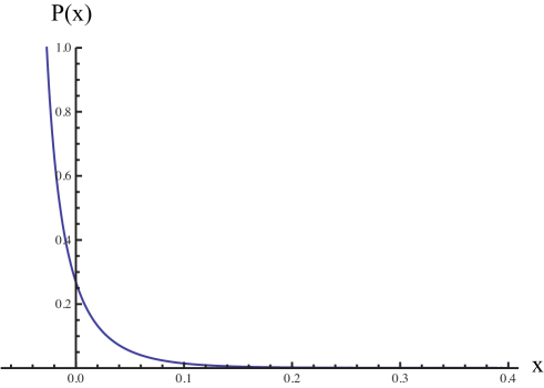
Figure 2: The graph of $P(x)$ vs $x$ of our fit to the probability distribution function for $\rho_{EM}$, the electromagnetic energy density sampled in time with a Lorentzian of width $\tau$. Here $x=16\pi^{2}\tau^{4}\,\rho_{EM}$. The distribution has an integrable singularity at the conjectured optimal quantum inequality bound $x=-x_{0}=-0.0472$.

Table 5: Fitting Constants for the Model Distribution for $\rho_{EM}$ in Eq. (81).

Constant	$\rho_{EM}$
$a$	0.9630614156
$c_{0}$	0.95539211
$x_{0}$	0.0472
$\alpha_{0}$	610
$c_{1}$	0.028
$\beta$	19.65
$\gamma$	1.05
$\alpha$	0.9999

Table 6: Table of Fractional Errors. Here the fractional error is $[a_{n}({\rm fit})-a_{n}]/a_{n}$, where the $a_{n}$ are given in Table 1 , and the $a_{n}(\rm fit)$ are computed from Eq. (81). For the $n=1$ case, the fractional error is not defined, since the first moment is 0. Fractional errors in succeeding moments beyond $n=5$ are progressively smaller. Although all moments through $n=65$ were used, we display the fractional errors through $n=21$.

$n$	$\rho_{EM}$
0	0.00450644
$1^{\rm st}$ moment	not applicable
2	-0.00661559
3	-0.0770297
4	-0.152164
5	-0.150279
6	-0.117773
7	-0.0843077
8	-0.0590582
9	-0.0420107
10	-0.0308225
11	-0.0233756
12	-0.0182526
13	-0.0145945
14	-0.0118911
15	-0.00983456
16	-0.0082327
17	-0.00696063
18	-0.00593416
19	-0.00509465
20	-0.00440012
21	-0.00381978

VI Bounds on the cumulative distribution function

As already mentioned, it is possible that the moment problem is indeterminate and that there are many probability distributions with these moments. Here, we show that no such distribution can have a tail decreasing much more slowly than that studied above. Our tool for this purpose is a simple variant of Chebyshev’s inequality: if $X$ is any random variable taking values in $[-x_{0},\infty)$, with moments $a_{n}$, then the probability $\text{Prob}(X\geq\lambda)$ that $X$ exceeds any given $\lambda$ is bounded by

$$\text{Prob}(X\geq\lambda)\leq\frac{a_{n}+\text{Prob}(X<0)x_{0}^{n}}{\lambda^{n}}$$ (82)

for all $n$. To prove this, let $d\mu(x)$ be the probability measure of $X$ and then compute

$$\lambda^{n}\text{Prob}(X\geq\lambda)=\lambda^{n}\int_{\lambda}^{\infty}d\mu(x)\leq\int_{\lambda}^{\infty}x^{n}d\mu(x)\leq\int_{0}^{\infty}x^{n}d\mu(x)=a_{n}-\int_{-x_{0}}^{0}x^{n}d\mu(x)\leq a_{n}+\text{Prob}(X<0)x_{0}^{n}.$$ (83)

(The term $\text{Prob}(X<0)x_{0}^{n}$ is only needed for odd $n$, in fact. We have also written $d\mu(x)$, rather than $P(x)dx$ for the probability measure to emphasise that we are not assuming a continuous probability density function.) In our case, we know that $x_{0}<x_{0}(FE)<1$, so we have

$$\text{Prob}(X\geq\lambda)\leq\inf_{n\in\mathbb{N}}\frac{a_{n}+1}{\lambda^{n}}.$$ (84)

Now, for moments growing as $a_{n}\sim CD^{n}(3n-4)!$, the ratio of successive terms in the infimum is

$$\frac{a_{n+1}+1}{\lambda(a_{n}+1)}\sim D\frac{(3n-1)(3n-2)(3n-3)}{\lambda},$$ (85)

so, for each fixed $\lambda$, the sequence will decrease until the term where $n\sim\frac{1}{3}(\lambda/D)^{1/3}$ and will increase thereafter. This gives an asymptotic bound on the tail probability

$$\text{Prob}(X\geq\lambda)\lesssim C\left(\frac{D}{\lambda}\right)^{\frac{1}{3}(\lambda/D)^{1/3}}\Gamma\left((\lambda/D)^{1/3}-3\right)\sim\sqrt{2\pi}C\left(\frac{D}{\lambda}\right)^{7/6}e^{-(\lambda/D)^{1/3}}.$$ (86)

as $\lambda\to\infty$.

This gives an upper bound on the tail probability distribution, which is not much more slowly decaying than that for our fitted tail, for which the tail probability would be decaying like $C\left(\frac{D}{\lambda}\right)^{4/3}e^{-(\lambda/D)^{1/3}}$. The following discussion sketches how information on the lower bound can be obtained; this could be developed into a rigorous discussion (and probably sharpened) with further work. In fact, we do not seek a strict lower bound on the tail probability, but rather aim to show that it must be very often of the order of the fitted tail or higher.

Let $Q(x)=\text{Prob}(X\geq x)$. Then we have, for any $\Lambda>\lambda>x_{0}$,

$$a_{n} \leq\lambda^{n}\text{Prob}(X<\lambda)+\int_{\lambda}^{\infty}x^{n}d\mu(x)$$ (87)

$$\leq\lambda^{n}\text{Prob}(X<\lambda)+Q(\lambda)\lambda^{n}+n\int_{\lambda}^{\infty}Q(x)x^{n-1}\,dx$$ (88)

$$\leq\lambda^{n}+n\int_{\lambda}^{\Lambda}Q(x)x^{n-1}\,dx+\sqrt{2\pi}CD^{n-1}n\int_{\Lambda}^{\infty}\left(\frac{x}{D}\right)^{n-13/6}e^{-(x/D)^{1/3}}\,dx$$ (89)

$$\leq\lambda^{n}+n\int_{\lambda}^{\Lambda}Q(x)x^{n-1}\,dx+3\sqrt{2\pi}CD^{n}n\Gamma(3n-7/2,(\Lambda/D)^{1/3})$$ (90)

in which we have integrated by parts in the second line and used the fact that $Q(\lambda)=1-\text{Prob}(X<\lambda)$, as well as the upper bound found above; $\Gamma(N,z)$ is the upper incomplete $\Gamma$-function. We can now make $n$-dependent choices of $\lambda$ and $\Lambda$ so that the first and third terms are negligible in comparison with $a_{n}$ for large enough $n$. For example, $\Lambda=(4n)^{3}D$ and $\lambda=n^{3}D$ will do: it is a simple application of Stirling’s formula to see that $\lambda^{n}/(D^{n}(3n-4)!)\sim\text{const}\times n^{7/2}(e/3)^{3n}\to 0$; for the upper end we first estimate $\Gamma(3n-7/2,4n)\sim 4(4n)^{3n-9/2}e^{-4n}$ using Laplace’s method (see deBruijn , section 4.3) which gives

$$n\frac{\Gamma(3n-7/2,4n)}{(3n-4)!}\sim\frac{1}{\sqrt{2\pi}}\left(\frac{3}{4}\right)^{7/2}\left(\frac{64}{27e}\right)^{n}\to 0.$$ (91)

With these choices of $\lambda$ and $\Lambda$ in force, we set $F(x)=xQ(x)e^{(x/D)^{1/3}}$, whereupon we have

$$n\int_{\lambda}^{\Lambda}F(x)x^{n-2}e^{-(x/D)^{1/3}}\,dx\gtrsim CD^{n}(3n-4)!$$ (92)

from (90). Now let $S$ be the subset of $x\in[\lambda,\Lambda]$ for which $F(x)\geq\frac{1}{2}CD(D/x)^{1/3}$. We bound $F$ from above by $\sqrt{2\pi}CD(D/x)^{1/6}$ on $S$, and by $\frac{1}{2}CD(D/x)^{1/3}$ on the complement $S^{c}$ of $S$ in $[\lambda,\Lambda]$, to give

$$\int_{\lambda}^{\Lambda}F(x)x^{n-2}e^{-(x/D)^{1/3}}\,dx\leq\sqrt{2\pi}CD^{7/6}\int_{S}x^{n-13/6}e^{-(x/D)^{1/3}}\,dx+\frac{CD^{4/3}}{2}\int_{S^{c}}x^{n-7/3}e^{-(x/D)^{1/3}}\,dx.$$ (93)

Now the first integral on the right-hand side can be bounded from above by the supremum of the integrand multiplied by the Lebesgue measure $|S|$ of $S$, while the second is bounded by the integral over all $[0,\infty)$. The supremum mentioned occurs for $x=(3n-13/2)^{3}D$, and we find

$$CD^{n}(3n-4)!\lesssim|S|\sqrt{2\pi}CD^{n-1}n(3n-13/2)^{3n-13/2}e^{-(3n-13/2)}+\frac{1}{2}CD^{n}3n\Gamma(3n-4).$$ (94)

Rearranging and using Stirling’s formula, this requires

$$|S|\gtrsim\frac{(3n-4)!e^{3n-13/2}D}{\sqrt{8\pi}n(3n-13/2)^{3n-13/2}}\sim\frac{27}{2}Dn^{2}.$$ (95)

Summarizing, we have shown that in the interval $[n^{3}D,4n^{3}D]$, for $n$ sufficiently large, we have

$$\text{Prob}(X\geq x)\geq\frac{1}{2}C\left(\frac{D}{x}\right)^{4/3}e^{-(x/D)^{1/3}}$$ (96)

on a set with measure at least $\frac{27}{2}Dn^{2}$. It seems likely that this is a substantial underestimate of the measure of $S$, as some of the estimates used in the last part of the argument are rather weak.

Thus the broad behavior of the tail of the probability distribution is determined by the moments, even if the exact probability distribution is not uniquely determined. In the applications we give below, it is only the broad behavior that is required.

VII Possible Applications for the Tail

VII.1 Black Hole Nucleation

The fact that the energy density probability distribution has a long positive tail implies a finite probability for the nucleation of black holes out of the Minkowski vacuum via large, though infrequent positive fluctuations. This probability cannot be too large, of course, or it will conflict with observation. Let us sample a spacetime region (a cell) over a size $\ell\approx\tau$, where $\tau$ equals the sampling time. For an energy density $\rho$, which is roughly constant in space, the associated mass will be $M\approx\rho{\ell}^{3}$. This can be a black hole if $GM\approx\ell$, or ${\ell_{p}}^{2}M\approx\ell$, in units where $\hbar=c=1$ and $\ell_{p}$ is the Planck length, which implies $\rho\approx 1/({\ell_{p}}^{2}{\ell}^{2})$. Here we chose $\tau\approx\ell$, so that the sampling time is approximately the light travel time across the black hole.

Note that we should really use the probability distribution for energy density sampled over a spacetime volume, with the spatial and temporal dimensions approximately equal. For the purpose of an order of magnitude estimate, we assume that the probability distribution for sampling in time alone will yield roughly similar results.

Let our observation volume be $V$ and our total observation time be $T$. The number of cells in this spacetime volume is $N=VT/{\ell}^{4}$. Because black hole nucleation will be a rare event, we assume that different nucleation events will be widely separated and uncorrelated. The number of black holes, $n$, nucleated in this spacetime volume, $VT$ is then $n\approx NP_{n}$, where $P_{n}$ is the probability of a black hole nucleation in our sampled spacetime volume ${\ell}^{4}$. Let us estimate that

$$P_{n}\approx\int_{x}^{2x}P(y)\,dy\,.$$ (97)

where

$$x=16\pi^{2}\tau^{4}\rho=16\pi^{2}\frac{\ell^{2}}{{\ell_{p}}^{2}}=16\pi^{2}{\Bigg{(}\frac{M}{m_{p}}\Bigg{)}}^{2}\,,$$ (98)

and $m_{p}$ is the Planck mass. Here $P_{n}$ is the probability of nucleating a black hole in the range between $x$ and $2x$. However, in the limit of large $x$, $P_{n}$ will be independent of the exact upper limit in Eq. (97). Let the probability distribution have a tail of the form given by Eq. (77). Then

$$P_{n}\approx c_{0}\int_{x}^{2x}y^{-2}\,e^{-ay^{1/3}}\,dy=3c_{0}a^{3}\int_{u_{1}}^{u_{2}}u^{-4}e^{-u}du=3\,c_{0}\,a^{3}[\Gamma(-3,u_{1})-\Gamma(-3,u_{2})]\,.$$ (99)

Here $u=ay^{1/3}$, $u_{1}=ax^{1/3}$, $u_{2}=2^{1/3}\,u_{1}$, and $\Gamma(-3,u)$ is an incomplete gamma function. This function has the asymptotic form

$$\Gamma(-3,u)\approx u^{-4}\,e^{-u}$$ (100)

for $u\gg 1$. From this form, we see that the contribution from the lower integration limit dominates, and we have

$$P_{n}\approx\frac{3\,c_{0}}{a}\,x^{-\frac{4}{3}}\,e^{-ax^{1/3}}$$ (101)

for large $x$.

Thus we have for the mean number of nucleated black holes

$$n=\frac{VT}{\ell^{4}}P_{n}=\frac{VT}{{\ell_{p}}^{8}M^{4}}P_{n}\,,$$ (102)

or, using Eq. (101),

$$n\approx\frac{3c_{0}}{a}\,(16\pi^{2})^{-4/3}\left(\frac{VT}{{\ell_{p}}^{4}}\right)\,{\Bigg{(}\frac{m_{p}}{M}\Bigg{)}}^{20/3}{\rm exp}[{-a_{0}{(M/m_{p})}^{2/3}}]\,,$$ (103)

where $a_{0}={(16\pi^{2})}^{1/3}a$. For the energy density of the EM field, $c_{0}\approx 0.955,\,a\approx 0.963$, so $a_{0}\approx 5.2$. Therefore for this case we have

$$n\approx 10^{-2}\,\Bigg{(}\frac{VT}{{\ell_{p}}^{4}}\Bigg{)}\,{\Bigg{(}\frac{m_{p}}{M}\Bigg{)}}^{20/3}{\rm exp}[{-5.2{(M/m_{p})}^{2/3}}]\,.$$ (104)

To estimate the probability of black hole nucleation, let us first choose $V=1{\rm cm}^{3}$, $T=1$ sec, and $n=1$, which gives $VT/{\ell_{p}}^{4}\approx{(10^{33})}^{3}\,10^{43}\approx 10^{142}$. We want the probability of one black hole forming in one cubic centimeter of space over an observation time of one second. We can use Eq. (104) to determine the resulting mass of the black hole, which turns out to be $M\approx 400\,m_{p}$. Let us now consider our observation volume and time to be the size and age of the universe, which gives $VT/{\ell_{p}}^{4}\approx{(10^{28}/10^{-33})}^{4}\approx 10^{244}$. Taking $n=1$ again, and using Eq. (104), yields $M\approx 990\,m_{p}$. Therefore, if we observe a volume the size of the universe for a time equal to the age of the universe, we are likely to see the nucleation of only about one $10^{3}m_{p}$ black hole from the vacuum.

Thus nucleation of black holes of mass $\sim 10^{2}\,m_{p}$ is common, but $10^{3}m_{p}$ black holes are very rare. Why do we not notice these $400\,m_{p}\approx 10^{-2}$ g black holes? Presumably they must appear for a very short time and be surrounded by negative energy which quickly destroys them.

VII.2 Boltzmann brains

Recently, the “Boltzmann brain” problem has become the subject of increasing interest in cosmology Bbrains ; Brains_olum . This is the possibility that conscious entities, which may or may not resemble biological brains, might spontaneously nucleate and exist for a finite time. Anthropic reasoning requires a count of observers, as the anthropic prediction for the value of an observable is the value most likely to be found by a typical observer. If the typical observer is a Boltzmann brain in intergalactic space, and not an observer on an earthlike planet, this would greatly alter anthropic predictions. As a somewhat more speculative application, we consider what the tails of our probability distributions have to say about the probability of nucleating Boltzmann brains in four-dimensional Minkowski spacetime. This calculation is similar to the one above for the nucleation of black holes.

Consider a spatial region of size $\ell$, a timescale $\tau$, and a mass $M$, so that the mean energy density is $\rho\approx M/{\ell}^{3}$. We want to use the tail of the EM energy density probability distribution to estimate the probability of mass $M$ appearing in this specific region in a particular interval $\tau$. Our sampled energy density is $x=16\pi^{2}{\tau}^{4}\,\rho\approx{\tau}^{4}\,M/{\ell}^{3}$. So we have that

$$P(x)\propto e^{-ax^{1/3}}\approx e^{-x^{1/3}}\approx{\rm exp}{\Bigg{(}-{\tau}^{\frac{4}{3}}\frac{M^{1/3}}{\ell}\Bigg{)}}\,$$ (105)

where we have ignored the prefactor and used $a\approx 1$. The prefactor would contain information about the fraction of mass $M$’s that could think. Even if very small, this factor is likely to pale in importance compared to the exponential factor derived below. Let $M=1\,{\rm kg}\approx 10^{41}\,{\rm cm}^{-1}$, $\ell=10$ cm, and $\tau=0.3\,{\rm sec}\approx 10^{10}$ cm. These values give

$${\tau}^{\frac{4}{3}}\frac{M^{1/3}}{\ell}\approx 10^{26}\,,$$ (106)

so

$$P\approx e^{-10^{26}}\,.$$ (107)

This is much larger than the ${\exp}(-10^{50})$ estimate of Page Page , who assumes that $P\propto e^{-I}$, where $I=Mt=$ action. So our energy density probability distribution makes the Boltzmann brain problem worse. Although the probability per unit volume for the nucleation of a Boltzmann brain may seem exceedingly low, the available volume could make them more numerous than other observers. Note that in this case, the energy density has been averaged over a spacetime region which is much larger in the time direction than in the spatial directions, $\tau\gg\ell$. Hence the probability distribution for the energy density averaged in time alone should be a good approximation here.

VIII Discussion

VIII.1 Uniqueness Issues

As was noted in Sec. III.2, the moments which we calculate for ${:}\dot{\varphi}^{2}{:}$ and related operators satisfy neither the Hamburger condition, Eq. (11), nor the Stieltjes condition, Eq. (47) for uniqueness. Thus none of our results for $P(x)$ are rigorously guaranteed to be unique. However, there are some observations which are relevant here. First, these are sufficient, but not necessary, conditions for uniqueness. There is a necessary and sufficient condition Simon , but this condition requires detailed knowledge of all moments and does not seem to be testable in our problem. Second, rapid growth of moments does not automatically mean non-uniqueness. There are examples of sets of moments which grow at arbitrary rates, but nonetheless are associated with unique probability distributions.

On the other hand, if the probability distribution is continuous, with probability density function $p(x)$ on $[-x_{0},\infty)$, and

$$\int_{-x_{0}}^{\infty}\frac{\log(p(x))\,dx}{\sqrt{x+x_{0}}(1+x)}>-\infty$$ (108)

then the Stieltjes problem is indeterminate for the moments of $p$ (assuming they all exist, and that $x_{0}<1$ for convenience); there is more than one probability distribution supported in $[-x_{0},\infty)$ with the same moments. This is a theorem of Krein (modified slightly to our setting) see, e.g., Theorem 5.1 in Ref. Berg . In particular, this would show that any distribution whose tail was exactly equal to $P_{\rm fit}(x)=c_{0}x^{-2}e^{-ax^{1/3}}$ for large enough $x$ had indeterminate moments in the above sense. On the other hand, if $p(x)$ were to oscillate around $P_{\rm fit}(x)$, but sometimes taking much smaller values than $P_{\rm fit}$, then the logarithm will take large negative values; such behavior could lead the integral to diverge and allow the moment problem to be determinate.

To illustrate how delicate the uniqueness issue can be, we note that the probability distribution $P(x)=\frac{1}{6}\theta(x)e^{-x^{1/3}}$, has moments $a_{n}=\frac{1}{2}(3n+2)!$, that are indeterminate in the Stieltjes sense on $[0,\infty)$ by Krein’s theorem. However, mild modifications of these moments yield determinate problems. For example, by Cor. 4.21 in Ref. Simon , there exists a constant $c$ so that the set of moments $\tilde{a}_{0}=1$, $\tilde{a}_{n}=c(3n-1)!$ is a determinate problem, corresponding to a purely discrete probability distribution.

Overall, we are not able to resolve the question of determinacy, although on balance our expectation is that the problem is indeed indeterminate. Certainly we have not been able to find any positive evidence to suggest that the moments are determinate. Nonetheless, certain features of the probability distribution can be ascertained. We have shown in Appendix A that our moments grow as a power times $(3n-4)!$. This rate of growth seems to be just what is needed to produce distributions with tails falling as in Eq. (77), that is, proportional to $x^{-2}e^{-ax^{1/3}}$. We have argued that any probability distribution arising from our moments will have a broadly similar tail. This asymptotic behavior is all that is needed for many applications of our distributions, such as those discussed in Sect. VII.

It is also worth noting that the conclusion that the probability distribution has a lower bound is independent of any concerns about uniqueness, because this follows from existing quantum inequality bounds. Our actual estimates of the lower bounds, given in Sect. IV, are not strictly independent of the uniqueness issue, but only use a finite number of the moments. Thus the numerical answers obtained only depend upon the values of these moments.

VIII.2 Summary

In this paper we have explored possible probability distributions for averaged quadratic operators in the four-dimensional Minkowski vacuum state. We use averaging with a Lorentzian function of time, and investigate the distributions for $\dot{\varphi}^{2}$, where $\varphi$ is a massless scalar field, for $\rho_{S}$, the associated scalar field energy density, for $E^{2}$, the squared electric field, and for $\rho_{EM}$. In all cases, we infer that the distributions have some features in common with our previous results FFR10 for a conformal field in two dimensions and for $\varphi^{2}$ in four dimensions. Specifically, there is a lower bound on the distribution, which coincides with the optimal quantum inequality bound on the associated expectation value in an arbitrary quantum state. Furthermore, there is no upper bound on the distributions, so arbitrarily large positive quantum fluctuations are possible.

We have outlined a procedure that, in principle, allows the calculation of an arbitrary number of moments of a given distribution. In practice, this procedure can be carried at least as far as the $65^{th}$ moment, which is sufficient to allow reasonable numerical estimates of both the lower bounds, and of the asymptotic tail for large argument. These are not guaranteed to be unique, but as was argued in the previous subsection, they may be useful.

If we accept the forms of the tails which we find, then several physically interesting applications follow, including the nucleation rates for black holes and Boltzmann brains. It should also be possible to apply these results to the study of the small scale structure of four dimensional spacetime, along the lines studied in two dimensions in Ref. CMP11 . It may also be possible to learn more about the non-Gaussian density and gravity wave perturbations in inflationary cosmology, which were studied in Refs. WKF07 ; FMNWW10 ; WHFN11 . Another implication of our form for the tail is that vacuum fluctuations will dominate thermal fluctuations at high energies. The Boltzmann distribution falls exponentially with energy, but vacuum energy density fluctuations fall more slowly and hence eventually dominate.

There is clearly room for further work on the topic of this paper. One obvious problem is to determine whether or not the moment problems we have studied are determinate: if so, one would like to know the detailed form of the corresponding probability distributions; if not, one would like to know how much information may be extracted from the moments, nonetheless, along the lines of the arguments in Sect. VI. In addition, our results have now trapped the sharp quantum inequality bounds for various operators between the lower bounds given by the methods of Ref. FewsterEveson98 and the bounds obtained in Sect. IV, which are an order of magnitude smaller. If the moment problem is determinate, the latter bounds will coincide with the sharp bound; otherwise it would be interesting to determine what the sharp bound actually is. Recall that here we deal only with Lorentzian sampling and only in the time direction. It will also be of interest to investigate more general sampling functions, and the effects of sampling in space as well as time.

Appendix A Computation of the moments

We describe how the moments of smeared Wick squares may be computed for a general derivative $\phi$ of the massless field $\varphi$ in four dimensions, writing $p$ for one more than twice the number of derivatives, so $p=1$ for ${:}\varphi^{2}{:}$ and $p=3$ for ${:}\dot{\varphi}^{2}{:}$. Thus the two-point function for $\phi$, restricted to the time axis, is given by

$$\langle\phi(t)\phi(t^{\prime})\rangle=\frac{1}{4\pi^{2}}\int_{0}^{\infty}d\omega\,\omega^{p}e^{-i\omega(t-t^{\prime}-i\epsilon)}\,.$$ (109)

With smearing along the time axis against smearing function $f$, the rules for computing the contribution to the $n$’th connected moment of a given connected graph on $n$ vertices may be stated in Fourier space as follows. For each line, the form of the two-point function entails that there is a momentum integral over the positive half-line and a factor of the $p$’th power of the momentum; for each vertex there is a factor of $\hat{f}(\omega_{j}+\omega_{k})$ if the vertex is the source of the lines carrying momenta $\omega_{j}$ and $\omega_{k}$, a factor of $\hat{f}(\omega_{j}-\omega_{k})$ if the vertex is the source (resp., target) of the line carrying momentum $\omega_{j}$ (resp., $\omega_{k}$), or a factor of $\hat{f}(-\omega_{j}-\omega_{k})$ if the vertex is the target of the lines carrying momenta $\omega_{j}$ and $\omega_{k}$; there is an overall factor of $(4\pi^{2})^{-n}$ and a combinatorial factor that is $2^{n}$ for $n\geq 3$ and $2$ for $n=2$. Here $\hat{f}$ is the Fourier transform, defined with the convention

$$\hat{f}(\omega)=\int_{-\infty}^{\infty}dtf(t)e^{i\omega t}\,.$$ (110)

An important point is that if, as for the Lorentzian, $\hat{f}$ is real and positive, then every graph contributes positively to the moment. Thus any individual graph on $n$-vertices gives a lower bound on the $n$’th connected moment. If one wishes to compute the dimensionless moments, defined in the text so that $a_{n}=(4\pi\tau^{(p+1)/2})^{2n}\mu_{n}$, the overall factor $2^{n}(4\pi^{2})^{-n}$ is replaced by $8^{n}\tau^{-(p+1)}$ for $n\geq 3$ (or $32$ in the case $n=2$).

In the particular case of the Lorentzian (9), we have $\hat{f}(\omega)={\rm e}^{-|\omega|\tau}$, and a simplification of the computation rules: a vertex met by lines carrying momenta $\omega_{j}$ and $\omega_{k}$ contributes ${\rm e}^{-|\omega_{j}-\omega_{k}|\tau}$ if it is a target for one and a source for the other, or $e^{-(\omega_{j}+\omega_{k})\tau}$ otherwise. This means that the overall integral over $\omega_{1},\ldots,\omega_{n}$ factorizes at each vertex that is either a double source or a double target.

Recall that the graphs involved are drawn on $n$ vertices $x_{1},\ldots,x_{n}$, placed in increasing order from left to right. Each vertex is met by two distinct lines, and each line is directed to the right. In particular, $x_{1}$ is the source of both lines connected to it. We may represent such a graph by a permutation $\sigma$ of the set $\{1,\ldots,n\}$ of integers, subject to the conditions that $\sigma(1)=1$ and $\sigma(2)<\sigma(n)$. To reconstruct a graph from a permutation, draw lines from $x_{1}=x_{\sigma(1)}$ to $x_{\sigma(2)}$, from $x_{\sigma(2)}$ to $x_{\sigma(3)}$, and so on, finishing with an line from $x_{\sigma(n)}$ to $x_{1}$. [For this reason, it is convenient to adopt a convention that $\sigma(n+1)=1$.] Then place rightwards-pointing arrows on each line. On the other hand, to encode a graph as a permutation, start at $x_{1}$ and follow the shorter of the two lines to the vertex it meets [i.e., of the two vertices joined to $x_{1}$, choose the one with the smaller label], and continue along the other line meeting that vertex. At each subsequent vertex, continue along the line not previously traversed, eventually returning to $x_{1}$. Then $\sigma(k)$ is defined to be the $k$’th vertex met on this trip.

A run of $\sigma$ is a set of consecutive integers in $\{1,\ldots,n+1\}$, say $p,p+1,\ldots q$, such that $\sigma(p),\sigma(p+1),\ldots,\sigma(q)$ is a monotone sequence, either ascending or descending, and so that no superset of consecutive integers has the same property. The length of the run is defined to be $q-p$. Every permutation used to label our graphs corresponds to an even number of runs, alternating between ascending and descending, whose lengths sum to $n$, and with consecutive runs sharing a common endpoint. For example, the permutation $14536782$ (i.e., $\sigma(1)=1$, $\sigma(2)=4$, $\sigma(3)=5$,…) has runs $1,2,3$; $3,4$; $4,5,6,7$ and $7,8,9$, of lengths $2,1,3,2$; representing each run by its image under the permutation, these runs are more transparently written as $145$, $53$, $3678$, $821$.

The contribution to the $n$’th connected moment arising from the graph corresponding to any given permutation is easily seen to factorize into terms corresponding to the runs, whose values depend only on the length of the run: in our example, the graph contributes $8^{8}K_{2}K_{1}K_{3}K_{2}=8^{8}K_{1}K_{2}^{2}K_{3}$ to the dimensionless connected moment $C_{8}$, where the $K_{j}$ correspond to the special case $K_{j}=K_{j}^{(0)}$ of the family of integrals

$$K_{n}^{(r)}=\frac{2^{r}}{r!}\int_{({\mathbb{R}}^{+})^{\times n}}dk_{1}\,dk_{2}\,\cdots dk_{n}k_{1}^{p+r}(k_{2}\cdots k_{n})^{p}e^{-k_{1}}e^{-\sum_{i=1}^{n-1}|k_{i+1}-k_{i}|}e^{-k_{n}}.$$ (111)

[Here, $k_{i}=\omega_{i}\tau$ are dimensionless versions of the momenta previously used.]

These considerations reduce the computation of the $n$’th connected moment to two problems: the computation of the $K_{j}$ and the enumeration of all permutations in the class considered with a given run structure. To address the first of these, we note the easily proved identity

$$\int_{0}^{\infty}dk\,k^{q}e^{-k}e^{-|k-\kappa|}=\frac{q!e^{-\kappa}}{2^{q+1}}\sum_{r=0}^{q+1}\frac{(2\kappa)^{r}}{r!},$$ (112)

of which the standard integral

$$\int_{0}^{\infty}dk\,k^{p}e^{-2k}=\frac{p!}{2^{p+1}}$$ (113)

is the $\kappa=0$ special case, and which entails the recurrence relation

$$K_{n}^{(r)}=\frac{p!}{2^{p+1}}\binom{p+r}{p}\sum_{r^{\prime}=0}^{p+r+1}K^{(r^{\prime})}_{n-1}.$$ (114)

As $K_{1}^{(r)}=2^{-(p+1)}p!\binom{p+r}{p}$, it follows that $K^{(r)}_{n}$ is given by

$$K_{n}^{(r)}=\left(\frac{p!}{2^{p+1}}\right)^{n}\binom{p+r}{p}\sum_{r_{n-1}=0}^{p+1+r}\sum_{r_{n-2}=0}^{p+1+r_{n-1}}\cdots\sum_{r_{1}=0}^{p+1+r_{2}}\prod_{k=1}^{n-1}\binom{p+r_{k}}{p}$$ (115)

for any integers $n\geq 1$ and $r\geq 0$. Although we have not found a closed form expression for the $K_{n}^{(r)}$, the above expressions allow for them to be computed efficiently.

To the best of our knowledge, the problem of enumerating permutations of the class we study in terms of their run structure does not appear to have been solved in the literature on enumerative combinatorics, although related problems have been studied for over a century. A closed form answer seems out of reach, but generating function techniques allow one to build up a solution for each $n$ in a recursive way. The details will be reported elsewhere Few_inprep , but the overall result is the following: for each $n$, let $\mathcal{K}_{n}$ be a polynomial in the variables $K_{1},\ldots,K_{n-1}$, with $\mathcal{K}_{2}=\frac{1}{2}K_{1}^{2}$ and subject to the recurrence relation

$$\mathcal{K}_{n}=\sum_{i}K_{i+1}\frac{\partial\mathcal{K}_{n-1}}{\partial K_{i}}+\sum_{i,j}K_{1}K_{i}K_{j}\frac{\partial\mathcal{K}_{n-1}}{\partial K_{i+j}}.$$ (116)

Then, for $n\geq 3$, the coefficient of $K_{1}^{m_{1}}\cdots K_{n-1}^{m_{n-1}}$ in $\mathcal{K}_{n}$ is precisely the number of permutations $\sigma$ of $\{1,\ldots,n\}$ with $m_{\ell}$ runs of length $\ell$ ($1\leq\ell\leq n-1$), subject to the side conditions $\sigma(1)=1$, $\sigma(2)<\sigma(n)$. In the case $n=2$, we find half of the number of such permutations.

The generating function is extremely convenient, because it already incorporates the sum over all possible connected graphs. Putting this together with the other considerations above, the $n$’th dimensionless connected moment is given by $C_{n}=8^{n}\mathcal{K}_{n}$, for any $n\geq 2$, where the variables $K_{j}$ are given the values defined above by (111) (recalling that $K_{j}=K_{j}^{(0)}$). For example, we find the explicit formulae:

$$C_{2} =32K_{1}^{2}$$ (117)

$$C_{3} =8^{3}K_{2}K_{1}$$ (118)

$$C_{4} =8^{4}\left(K_{3}K_{1}+K_{2}^{2}+K_{1}^{4}\right)$$ (119)

$$C_{5} =8^{5}\left(K_{4}K_{1}+3K_{3}K_{2}+8K_{2}K_{1}^{3}\right)$$ (120)

$$C_{6} =8^{6}\left(K_{5}K_{1}+3K_{3}^{2}+4K_{4}K_{2}+13K_{3}K_{1}^{3}+31K_{2}^{2}K_{1}^{2}+8K_{1}^{6}\right)$$ (121)

$$C_{7} =8^{7}\left(K_{6}K_{1}+10K_{4}K_{3}+5K_{5}K_{2}+19K_{4}K_{1}^{3}+66K_{2}^{3}K_{1}+123K_{3}K_{1}^{2}K_{2}+136K_{2}K_{1}^{5}\right)$$ (122)

which can be used to provide the first few connected moments for ${:}\varphi^{2}{:}$ in the case $p=1$ or ${:}\dot{\varphi}^{2}{:}$ in the case $p=3$. One may check that the coefficients inside each parenthesis sum to $(n-1)!/2$, the total number of connected graphs involved in the $n$’th moment.

Appendix B Asymptotics of the moments

In this appendix we give asymptotic estimates for the $n$’th moments of the Lorentzian smearing of the Wick square of the $\frac{1}{2}(p-1)$’th derivative of $\varphi$ as $n$ becomes large. We rigorously establish a lower bound and also give an upper bound, for which our reasoning is not completely rigorous, but which appears to be satisfied on the grounds of numerical evidence. The basic observation is that the dominant contribution to $C_{n}$ [and hence the full dimensionless moment $a_{n}$] is $8^{n}K_{n-1}K_{1}$; this is certainly a lower bound (as all terms are positive) and numerical evidence suggests that it gives the correct answer modulo a fractional error of order $n^{-2}$. Thus lower bounds on the $K_{j}$ will give rigorous lower bounds on $C_{n}$, while upper bounds give an upper bound on the $C_{n}$ that seems reasonably secure, albeit not fully rigorous. In terms of permutations and graphs, the dominant contribution arises from the identity permutation, and thus the graph on $n$ vertices that has lines from $x_{k}$ to $x_{k+1}$ for each $k=1,\ldots,n-1$ and an line from $x_{1}$ to $x_{n}$. The graphs in Fig. 1 represent the case $n=2$ and $n=3$.

We begin with the lower bound, which is

$$K^{(r)}_{n}\geq\binom{n(p+1)-1+r}{n(p+1)-1}L^{(r)}_{n},$$ (123)

where

$$L^{(r)}_{n}=\frac{(n(p+1))!}{n!(2^{p+1}(p+1))^{n}}\prod_{k=1}^{n-1}\frac{r+n(p+1)}{r+k(p+1)},$$ (124)

in which the product over $k$ is taken to be equal to unity in the case $n=1$. The bound (123) is proved by induction, noting that the it is true (indeed, an equality) for $n=1$. Supposing that it holds for some $n\geq 1$, we use the recurrence relation Eq. (114) to show that

$$K^{(r)}_{n+1} \geq\frac{p!}{2^{p+1}}\binom{p+r}{p}\binom{(n+1)(p+1)+r}{n(p+1)}L_{n}^{(p+1+r)}$$

$$=\frac{p!}{2^{p+1}}\frac{r+(n+1)(p+1)}{r+p+1}\binom{(n+1)(p+1)-1}{p}\binom{(n+1)(p+1)-1+r}{(n+1)(p+1)-1}L_{n}^{(p+1+r)},$$ (125)

where, in the first line, we have used the fact that the constants $L^{(r)}_{n}$ are clearly monotone decreasing in $r$ for each fixed $n$, and the identity (0.151.1 in Ref. GR )

$$\sum_{r=0}^{R}\binom{q+r}{q}=\binom{q+1+R}{q+1};$$ (126)

the second line is an elementary algebraic manipulation. A further algebraic manipulation shows that

$$L_{n+1}^{(r)}=\frac{p!}{2^{p+1}}\frac{r+(n+1)(p+1)}{r+p+1}\binom{(n+1)(p+1)-1}{p}L_{n}^{(p+1+r)}$$ (127)

which allows us to conclude that the bound on $K_{n}^{(r)}$ holds for all $n$ by induction. Noting that

$$L_{n}^{(0)}=\frac{(n(p+1))!n^{n}}{(2^{(p+1)}(p+1))^{n}(n!)^{2}}$$ (128)

we obtain a lower bound on $J_{n}=K_{1}^{(0)}K_{n-1}^{(0)}=p!2^{-(p+1)}K^{(0)}_{n-1}$ as

$$J_{n}\geq\frac{p!}{2^{p+1}}L^{(0)}_{n-1}=\frac{(p+1)!((n-1)(p+1))!(n-1)^{n-1}}{(2^{p+1}(p+1))^{n}((n-1)!)^{2}}.$$ (129)

In a similar way, we find an upper bound

$$K_{n}^{(r)}\leq\binom{n(p+2)-2+r}{n(p+1)-1}U^{(r)}_{n}$$ (130)

where

$$U_{n}^{(r)}=\frac{(n(p+1))!}{n!(2^{p+1}(p+1))^{n}}\prod_{k=0}^{n-2}\prod_{q=1}^{p}\frac{k(p+1)+r+q}{kp+r+n+q-1}$$ (131)

and the product on $k$ is again regarded as a factor of unity in the case $n=1$. From this expression, it is clear that the $U_{n}^{(r)}$ are monotone increasing in $r$ for each fixed $n$. The double product can be also be written as a ratio of products of $\Gamma$-functions and other simple functions; in the case $r=0$ there is a particularly simple expression

$$\prod_{k=0}^{n-2}\prod_{q=1}^{p}\frac{k(p+1)+q}{kp+n+q-1}=(p+1)^{1-n}.$$ (132)

As before, we prove (130) by induction, noting that it holds with equality in the case $n=1$. Supposing that it is true for some $n\geq 1$, the recurrence relation Eq. (114) gives

$$K_{n+1}^{(r)}\leq\frac{p!}{2^{p+1}}\binom{p+r}{p}\sum_{r^{\prime}=0}^{p+r+1}\binom{n(p+2)-2+r^{\prime}}{n(p+1)-1}U^{(r^{\prime})}_{n}.$$ (133)

Over the summation range, we have $U^{(r^{\prime})}_{n}\leq U^{(p+1+r)}_{n}$, so

$$K_{n+1}^{(r)}\leq U^{(p+1+r)}_{n}\frac{p!}{2^{p+1}}\binom{p+r}{p}\sum_{r^{\prime}=0}^{p+r+1}\binom{n(p+2)-2+r^{\prime}}{n(p+1)-1}\leq U^{(p+1+r)}_{n}\binom{p+r}{p}\frac{p!}{2^{p+1}}\sum_{r^{\prime\prime}=0}^{p+r+n}\binom{n(p+1)-1+r^{\prime\prime}}{n(p+1)-1},$$ (134)

where we have changed summation variable to $r^{\prime\prime}=r^{\prime}+n-1$ and extended the summation range in the second step. Using Eq. (126), this gives

$$K_{n+1}^{(r)}\leq\frac{p!}{2^{p+1}}\binom{p+r}{p}\binom{n(p+2)+p+r}{n(p+1)}U^{(p+1+r)}_{n}$$ (135)

Using the fact that

$$\binom{p+r}{p}\binom{n(p+2)+p+r}{n(p+1)}=\frac{((n+1)(p+1))!}{(n+1)(p+1)[n(p+1)]!p!}\binom{(n+1)(p+2)-2+r}{(n+1)(p+1)-1}\prod_{q=1}^{p}\frac{r+q}{r+n+q},$$ (136)

it is then easy to show that (130) holds with $n$ replaced by $n+1$ and hence for all $n$ by induction.

We may then obtain the upper bound on $J_{n}$ as

$$J_{n}\leq\frac{(p+1)!(p+1)^{3}}{(2^{p+1}(p+1)^{2})^{n}}\frac{((n-1)(p+2)-2)!}{((n-2)!)^{2}}$$ (137)

after some manipulation.

Using Stirling’s formula, $(nA-B)!\sim\sqrt{2\pi}(nA/e)^{nA-B+1/2}e^{-B+1/2}$. Then one may check that the lower bound in (129) is, asymptotically,

$$J_{n}\gtrsim\frac{(p+1)!}{2\pi e}\left(\frac{p}{p+1}\right)^{p+1/2}\left(\frac{(p+1)^{p}e}{p^{p}2^{p+1}}\right)^{n}(np-(p+1))!$$ (138)

while a similar calculation at the upper bound gives

$$J_{n}\lesssim\frac{(p+1)!(p+1)^{3}}{2\pi(p+2)^{3}}\left(\frac{p}{p+2}\right)^{p+1/2}\left(\frac{(p+2)^{p+2}}{2^{p+1}(p+1)^{2}p^{p}}\right)^{n}(np-(p+1))!$$ (139)

so the ratio of the upper bound to the lower bound grows as $\sim\alpha\beta^{n}$ as $n\to\infty$, with

$$\alpha=e\left(\frac{p+1}{p+2}\right)^{p+7/2},\qquad\beta=\frac{1}{e}\left(\frac{p+2}{p+1}\right)^{p+2},$$

which in the case $p=3$ gives $\alpha=0.6373520649$, $\beta=1.122678959$. So we have a reasonable control over the leading order contribution.

As mentioned above, it is certain that the dimensionless moment $a_{n}$ obeys $a_{n}\geq 8^{n}J_{n}$, and numerical evidence suggests that $a_{n}\sim 8^{n}J_{n}$ at least in the case $p=3$ (we believe that this is true for all $p>1$ and could be proved with more effort). On that basis, we have

$$0.513395\times 3.221667^{n}\lesssim\frac{a_{n}}{(3n-4)!}\lesssim 0.327213\times 3.616898^{n}$$ (140)

in the $p=3$ case, for $n\to\infty$. This supports the growth estimates given in the text.

References

- (1) See, for example, N.D. Birrell and P.C.W. Davies, Quantum Fields in Curved Space, (Cambridge University Press, 1982), Chap. 8.
- (2) C.-H. Wu and L.H. Ford, Phys. Rev. D 64, 045010 (2001), quant-ph/0012144.
- (3) J. Borgman and L.H. Ford, Phys. Rev. D 70 064032 (2004), gr-qc/0307043.
- (4) B.L. Hu and E. Verdaguer, Living Rev. Rel. 7, 3 (2004), gr-qc/0307032.
- (5) L.H. Ford and R.P. Woodard, Class. Quant. Grav. 22, 1637 (2005), gr-qc/0411003.
- (6) R.T. Thompson and L.H. Ford, Phys. Rev. D 74, 024012 (2006), gr-qc/0601137.
- (7) G. Perez-Nadal, A. Roura and E. Verdaguer, JCAP 1005, 036 (2010), arXiv:0911.4870
- (8) L.H. Ford and C.H. Wu, AIP Conf.Proc. 977 145 (2008), arXiv:0710.3787.
- (9) E. Calzetta and S. Gonorazky, Phys. Rev. D 55, 1812 (1997).
- (10) C.-H. Wu, K.-W. Ng, and L.H. Ford, Phys. Rev. D 75, 103502 (2007), arXiv:gr-qc/0608002.
- (11) L.H. Ford, S.-P. Miao, K.-W. Ng, R.P. Woodard, and C.-H. Wu, Phys. Rev. D 82, 043501 (2010), arXiv:1005.4530.
- (12) C.-H. Wu, J.-T. Hsiang, L. H. Ford, and K.-W. Ng, Phys. Rev. D 84, 103515 (2011), arXiv:1105.1155.
- (13) F. Lombardo and D. Nacir, Phys. Rev. D 72, 063506 (2005).
- (14) C.H. Wu, K.W. Ng, W. Lee, D.S. Lee, and Y.Y. Charng, JCAP 0702, 006 (2007).
- (15) C.J. Fewster, L.H. Ford, and T.A. Roman, Phys. Rev. D 81, 121901(R) (2010), arXiv:1004.0179.
- (16) G. Duplancic, D. Glavan, and H. Stefancic, Phys. Rev. D 82, 125008 (2010), arXiv:1002.1846.
- (17) M. Reed and B. Simon, Methods of modern mathematical physics II: Fourier analysis, self-adjointness (Academic Press, New York, 1975).
- (18) K. Sanders, arXiv:1010.3978.
- (19) B. Simon, Adv. Math. 137, 82 (1998).
- (20) S. Carlip, R. A. Mosna, and J. P. M. Pitelli, Phys. Rev. Lett. 107, 021303 (2011), arXiv:1103.5993.
- (21) L. H. Ford, Proc. Roy. Soc. Lond. A 364, 227 (1978).
- (22) L. H. Ford, Phys. Rev. D 43, 3972 (1991).
- (23) L.H. Ford and T.A. Roman, Phys. Rev. D 51, 4277 (1995), gr-qc/9410043.
- (24) L.H. Ford and T.A. Roman, Phys. Rev. D 55, 2082 (1997), gr-qc/9607003.
- (25) E.E. Flanagan, Phys. Rev. D 56, 4922 (1997), gr-qc/9706006.
- (26) C.J. Fewster and S. Hollands, Rev. Math. Phys. 17, 577 (2005), math-ph/0412028.
- (27) C.J. Fewster and S.P. Eveson, Phys. Rev. D 58, 084010 (1998), gr-qc/9805024.
- (28) L.H. Ford, A. D. Helfer, and T. A. Roman, Phys. Rev. D 66, 124012 (2002), gr-qc/0208045.
- (29) L.H. Ford and T.A. Roman, Phys. Rev. D 53, 5496 (1996), gr-qc/9510071.
- (30) M.J. Pfenning and L.H. Ford, Class. Quant. Grav. 14, 1743 (1997), gr-qc/9702026.
- (31) See the ancillary files for the full list of , , , , and moments up through .
- (32) N.G. de Bruijn, Asymptotic methods in analysis (Dover, 1981).
- (33) A. De Simone, A.H. Guth, A. Linde, M. Noorbala, M.P. Salem, and A. Vilenkin, Phys. Rev. D 82, 063520 (2010), arXiv:0808.3778.
- (34) M. Davenport and K.D. Olum, arXiv:1008.0808.
- (35) D. Page, J. Kor. Phy. Soc. 49, 711 (2006); hep-th/0510003.
- (36) C. Berg, J. Comput. Appl. Math. 65, 27 (1995).
- (37) C.J. Fewster, in preparation.
- (38) I.S. Gradshteyn and I.M. Rhyzik, Table of integrals, series and products 5th edition. Translation edited and with a preface by Alan Jeffrey (Academic Press, 1994).