Anisotropic Compact stars with variable cosmological constant

Abstract

Recently the small value of the cosmological constant and its ability to accelerate the expansion of the Universe is of great interest. We discuss the possibility of forming of anisotropic compact stars from this cosmological constant as one of the competent candidates of dark energy. For this purpose we consider the analytical solution of Krori and Barua metric. We take the radial dependence of cosmological constant and check all the regularity conditions, TOV equations, stability and surface redshift of the compact stars. It has been shown as conclusion that this model is valid for any compact star and we have cited $4U~{}1820-30$ as a specific example of that kind of star.

Managing Editor

1 Introduction

The study of general relativistic compact objects is of great interest for a long time. The theoretical investigation of superdense stars has been done by several authors using both analytical and numerical methods. [2] emphasized on the importance of locally anisotropic equations of state for relativistic fluid spheres for generalizing the equations of hydrostatic equilibrium to include the effects of local anisotropy. They showed that anisotropy may have non-negligible effects on such parameters like maximum equilibrium mass and surface redshift. [24] has investigated the stellar models and argued that the nuclear matter may have anisotropic features at least in certain very high density ranges ($>~{}10^{15}$gm/c.c.), where the nuclear interaction must be treated relativistically.

Einstein introduced the cosmological constant into his field equations to make them consistent with Mach’s principle and to get a non-expanding static solutions of the Universe. If matter is the source of inertia, then in absence of it there should not be any inertia. In view of that he introduced the cosmological constant $\Lambda$ to eliminate inertia when matter is absent [8]. With the successes of FRW cosmology and later on experimental verification of expanding Universe by Hubble the idea of $\Lambda$ was abandoned by Einstein himself.

However, in modern cosmology, recent measurement conducted by WMAP indicates that $73\%$ of the total mass-energy of the Universe is dark energy [18, 23]. Dark energy theory is therefore thought to be the most acceptable one to explain the present phase of the accelerated expansion of the Universe. The erstwhile Cosmological constant adopted by Einstein is a good candidate to explain this dark energy in the cosmological realm. However, even in the astrophysical point of view we would like to go back to the idea of [8] that $\Lambda$ has something common in matter distribution.

As a start of the astrophysical objects of compact nature (either as neutron stars or strange stars or others) let us mention some of the important works done by [6], [7] and [4] where $\Lambda$ have taken as a source of matter distribution of the stars. [14] have calculated the mass-radius ratio for compact relativistic star in the presence of cosmological constant. On the other hand, anisotropy have been introduced as key feature in the configuration of the compact stars which enabled several investigators to model the objects physically more viable [26, 20, 21, 22, 17]. In the studies of compact stars some other notatble works with different aspects are as follows: [5], [12, 13], [Mak2002, Mak2003], [25].

Motivating with the above investigations we take the cosmological constant as a source of matter and study the structure of compact stars and arrived at the conclusion that incorporation of $\Lambda$ describes the well known compact stars, for examples neutron stars, white dwarf stars, X ray buster 4U 1820-30, Millisecond pulsar SAX J 1808.4-3658 etc., in a good manner. In this article, therefore, we have proposed a model for anisotropic compact stars which satisfies all the energy conditions, TOV-equations and other physical requirements. We also investigate the stability, mass-radius relation and surface redshifts for our model and found that their behaviour is well matched with the compact stars.

2 Non-singular Model for Anisotropic Compact Stars

The general line element for a static spherically symmetric space-time in [11] model (henceforth KB) is given by

$$ds^{2}=-e^{\nu(r)}dt^{2}+e^{\lambda(r)}dr^{2}+r^{2}(d\theta^{2}+sin^{2}\theta d\phi^{2}),$$ (1)

with $\lambda(r)=Ar^{2}$ and $\nu(r)=Br^{2}+C$ where $A$, $B$ and $C$ are arbitrary constants to be determined on physical grounds. The interior of the anisotropic compact star may be expressed in the standard form as

$$T_{ij}=diag(\rho,-p_{r},-p_{t},-p_{t}),$$

where $\rho$, $p_{r}$ and $p_{t}$ correspond to the energy density, normal pressure and transverse pressure respectively.

We take the cosmological constant as radial dependence i.e. $\Lambda~{}=~{}\Lambda(r)~{}=~{}\Lambda_{r}$ (say). Therefore, the Einstein field equations for the metric (1) are obtained as (where natural units $G=c=1$)

$$8\pi\rho+\Lambda_{r} = e^{-\lambda}\left(\frac{\lambda^{\prime}}{r}-\frac{1}{r^{2}}\right)+\frac{1}{r^{2}},$$ (2)

$$8\pi p_{r}-\Lambda_{r} = e^{-\lambda}\left(\frac{\nu^{\prime}}{r}+\frac{1}{r^{2}}\right)-\frac{1}{r^{2}},$$ (3)

$$8\pi\ p_{t}-\Lambda_{r} = \frac{e^{-\lambda}}{2}\left[\frac{{\nu^{\prime}}^{2}-\lambda^{\prime}\nu^{\prime}}{2}+\frac{\nu^{\prime}-\lambda^{\prime}}{r}+\nu^{\prime\prime}\right].$$ (4)

To get the physically acceptable stellar models, we propose that the radial pressure of the compact star is proportional to the matter density i.e.

$$p_{r}=m\rho,~{}~{}~{}m>0,$$ (5)

where $m$ is the equation of state parameter.

Now, from the metric (1) and equations (2) - (5), we get the energy density $\rho$, normal pressure $p_{r}$, tangential pressure $p_{t}$ and cosmological parameter $\Lambda_{r}$, respectively as

$$\rho = \frac{2(A+B)}{8\pi(m+1)}e^{-Ar^{2}}>0,$$ (6)

$$p_{r} = \frac{m(A+B)}{4\pi(m+1)}e^{-Ar^{2}}>0,$$ (7)

$$p_{t} = \frac{1}{8\pi(m+1)}[e^{-Ar^{2}}((m+1)(B^{2}-AB)r^{2}$$ (8)

$$+m(2B+A)-A-\frac{(m+1)}{r^{2}})+\frac{(m+1)}{r^{2}}].$$

$$\Lambda_{r} = \frac{e^{-Ar^{2}}}{m+1}\left[2(Am-B)-\frac{m+1}{r^{2}}\right]+\frac{1}{r^{2}}.$$ (9)

Also, the equation of state (EOS) parameters corresponding to normal and transverse directions can be written as

$$\omega_{r}(r)=m,$$ (10)

$$\omega_{t}(r)=\frac{1}{2(A+B)}\left[\frac{e^{Ar^{2}}(m+1)}{r^{2}}-\frac{(m+1)}{r^{2}}\right.$$

$$\left.+(m+1)(B^{2}-AB)r^{2}+m(2B+A-\frac{A}{m})\right].$$ (11)

3 Physical Analysis

In this section we will discuss the following features of our model:

3.1 Anisotropic Behavior

From the equations (6) and (7) we have

$$\frac{d\rho}{dr}=-\left[\frac{A(A+B)}{2\pi(m+1)}re^{-Ar^{2}}\right]<0,$$

and

$$\frac{dp_{r}}{dr}<0.$$

The above results and Figs. (1) and (2) conclude that, at $r=0$, our model provides

$$\frac{d\rho}{dr}=0,~{}~{}\frac{dp_{r}}{dr}=0,$$

$$\frac{d^{2}\rho}{dr^{2}}=-\frac{A(A+B)}{2\pi(m+1)}<0,$$

and

$$\frac{d^{2}p_{r}}{dr^{2}}=-\frac{mA(A+B)}{2\pi(m+1)}<0.$$

which indicate maximality of central density and central pressure.

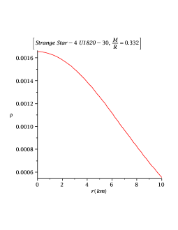
Figure 1: Density variation at the stellar interior of Strange star candidate $4U~{}1820-30$

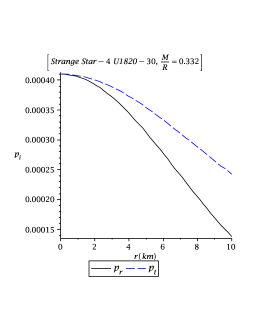
Figure 2: Radial and Transverse Pressure variation at the stellar interior of Strange star candidate $4U~{}1820-30$

It is interesting to note that, like normal matter distribution, the bound on the effective EOS in this construction is given by $0<\omega_{i}(r)<1$, (see Fig. (3)) despite of the fact that star is constituted by the combination of ordinary matter and effect of $\Lambda$. Here figures are drawn taking m=$\frac{1}{3}$.

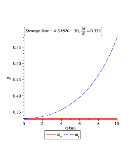
Figure 3: Variation of equation of state parameter with distance of Strange star candidate $4U~{}1820-30$

The measure of anisotropy, $\Delta=\frac{2}{r}\left(p_{t}-p_{r}\right)$, in this model is obtained as

$$\Delta=\frac{1}{4\pi r}\left[e^{-Ar^{2}}\left((B^{2}-AB)r^{2}-A-\frac{1}{r^{2}}\right)+\frac{1}{r^{2}}\right].$$ (12)

The ‘anisotropy’ will be directed outward when $P_{t}>P_{r}$ i.e. $\Delta>0$, and inward when $P_{t}<P_{r}$ i.e. $\Delta<0$. It is apparent from the Fig. (4) of our model that a repulsive ‘anisotropic’ force ($\Delta>0$) allows the construction of more massive distributions.

Figure 4: Comparison of anisotropic behaviours at the stellar interior of Strange star candidates $4U~{}1820-30$, $Her~{}X-1$ and $SAX~{}J~{}1808.4-3658$

3.2 Matching Conditions

Here we match the interior metric to the Schwarzschild exterior

$$ds^{2}=-\left(1-\frac{2M}{r}\right)dt^{2}+\left(1-\frac{2M}{r}\right)^{-1}dr^{2}$$

$$+r^{2}(d\theta^{2}+\sin^{2}\theta d\phi^{2}),$$ (13)

at the boundary $r=b$ (radius of the star). Assuming the boundary conditions $p_{r}(r=b)=0$ and $\rho(r=0)=\rho_{0}$, where $\rho_{0}$ is the central density, we have

$$A = \frac{8\pi\rho_{0}}{3},$$ (14)

$$B = \frac{1}{2b^{2}}\left[e^{\frac{8\pi\rho_{0}}{3}b^{2}}-1\right].$$ (15)

Table 1: Values of the model parameters for different Strange stars.

Strange Quark Star	$M$($M_{\odot}$)	$R$(km)	$\frac{M}{R}$	$A$ (km-2)	$B$ (km-2)	$\rho_{0}$(km-2)
Her X-1	0.88	7.7	0.168	0.006906276428	0.004267364618	0.0008247941592
SAX J 1808.4-3658(SS1)	1.435	7.07	0.299	0.01823156974	0.01488011569	0.002177337150
4U 1820-30	2.25	10.0	0.332	0.01090644119	0.009880952381	0.001302520843

At this juncture, let us first evaluate some reasonable set for values of $A$ and $B$. According to [3], the maximum allowable compactness (mass-radius ratio) for a fluid sphere is given by $\frac{2M}{R}<\frac{8}{9}$. Values of the model parameters for different Strange stars (Table 1) show the acceptability of our model.

We have also verified with different sets of mass and radius leading to solutions for the unknown parameters which satisfy the following conditions through out the configuration:

$$\rho\geq 0,~{}~{}~{}\rho+p_{r}\geq 0,~{}~{}~{}\rho+p_{t}\geq 0,~{}~{}~{}\rho+p_{r}+2p_{t}\geq 0,$$

$\rho>|p_{r}|$ and $\rho>|p_{t}|$.

Null Energy Condition (NEC), Weak Energy Condition (WEC), Strong Energy Condition (SEC) and Dominant Energy Condition (DEC) i.e. all the energy conditions for our particular choices of the values of mass and radius are satisfied.

The anisotropy, as expected, vanishes at the centre, i.e. $r=0$, $p_{t}=p_{r}=p_{0}=\frac{m(A+B)}{4\pi(m+1)}$. The energy density and the two pressures are also well behaved in the interior of the stellar configuration.

3.3 Matter Density and Pressure

From the equations (6), (14) and (15) we have

$$\rho=\rho_{0}e^{(-\frac{8\pi\rho_{0}}{3})r^{2}}.$$

Since it is well known that $0<m<1$ and $\frac{M}{R}~{}<~{}\frac{4}{9}$ for a compact star with radius $R$ and mass $M$, hence our model suggests a range for matter density of the star, which is

$$e^{-Ab^{2}}\frac{A+B}{8\pi}~{}<\rho~{}<\frac{3}{\pi b^{2}}.$$

According to the equation (5), i.e. $p_{r}=m\rho$, the pressure will vary linearly with the density and the range of the pressure will differ from density with just by a factor of radial equation state parameter. It is then clear from the Table 1 along with the Figs. (1) and (2) that our bound is justified.

3.4 TOV Equation

For an anisotropic fluid distribution, the generalized TOV equation is given by

$$\frac{d}{dr}\left(p_{r}-\frac{\Lambda_{r}}{8\pi}\right)+\frac{1}{2}\nu^{\prime}\left(\rho+p_{r}\right)+\frac{2}{r}\left(p_{r}-p_{t}\right)=0.$$ (16)

Following Ponce de León [19], we write the above TOV equation as

$$-\frac{M_{G}\left(\rho+p_{r}\right)}{r^{2}}e^{\frac{\lambda-\nu}{2}}-\frac{d}{dr}\left(p_{r}-\frac{\Lambda_{r}}{8\pi}\right)+\frac{2}{r}\left(p_{t}-p_{r}\right)=0,$$ (17)

where $M_{G}=M_{G}(r)$ is the gravitational mass inside a sphere of radius $r$ and is given by

$$M_{G}(r)=\frac{1}{2}r^{2}e^{\frac{\nu-\lambda}{2}}\nu^{\prime},$$ (18)

which can easily be derived from the Tolman-Whittaker formula and the Einstein field equations. Obviously, the modified TOV equation describes the equilibrium condition for the compact star subject to the gravitational and hydrostatic plus another force due to the anisotropic nature of the stellar object. Now, the above equation can be written as

$$F_{g}+F_{h}+F_{a}=0,$$ (19)

where

$$F_{g} = -Br\left(\rho+p_{r}\right),$$ (20)

$$F_{h} = -\frac{d}{dr}\left(p_{r}-\frac{\Lambda_{r}}{8\pi}\right)$$ (21)

$$= \frac{re^{-Ar^{2}}}{4\pi(m+1)}\left[(m+1)\left(\frac{1}{Ar^{4}}+\frac{1}{r^{2}}\right)\right.$$

$$\left.+2B(mA+1)+2mA(A-1)\frac{}{}\right]-\frac{1}{4\pi r^{3}},$$

$$F_{a} = \frac{2}{r}\left(p_{t}-p_{r}\right).$$ (22)

Note that here the variable $\Lambda$ contributes to the hydrostatic force. The profiles of $F_{g}$, $F_{h}$ and $F_{a}$ for our chosen source are shown in Fig. 5. The figure indicates that the static equilibrium is attainable due to the combined effect of pressure anisotropy, gravitational and hydrostatic forces.

Figure 5: Behaviours of pressure anisotropy, gravitational and hydrostatic forces at the stellar interior of Strange star candidate $4U~{}1820-30$

3.5 Stability

In our anisotropic model, we define sound speeds as

$$v_{sr}^{2}~{}=~{}m,$$ (23)

$$v^{2}_{st}=\frac{dp_{t}}{d\rho}=\frac{(m+1)}{2A(A+B)}\left[\frac{e^{Ar^{2}}}{r^{4}}+A(B^{2}-AB)r^{2}\right.$$

$$\left.-((B^{2}-AB)+\frac{A^{2}-Am(2B+A)}{(m+1)})-\frac{A}{r^{2}}-\frac{1}{r^{4}}\right].$$ (24)

We plot the radial and transverse sound speeds in the Fig. 6 and observe that these parameters satisfy the inequalities $0\leq v_{sr}^{2}\leq 1$ and $0\leq v_{st}^{2}\leq 1$ everywhere within the stellar object which obeys the anisotropic fluid models [9, 1].

The above equations (23) and (24) therefore lead to

$$v^{2}_{st}-v^{2}_{sr}=\frac{(m+1)}{2A(A+B)}\left[\frac{e^{Ar^{2}}}{r^{4}}+A(B^{2}-AB)r^{2}\right.$$

$$\left.-\left((B^{2}-AB)+\frac{A^{2}-Am(2B+A)}{(m+1)}\right)-\frac{A}{r^{2}}-\frac{1}{r^{4}}\right]-m$$ (25)

From the Fig. (7), we can easily say that $v^{2}_{st}-v^{2}_{sr}\leq 1$. Since, $0\leq v_{sr}^{2}\leq 1$ and $0\leq v_{st}^{2}\leq 1$, therefore, $\mid v_{st}^{2}-v_{sr}^{2}\mid\leq 1$.

Again, to check whether local anisotropic matter distribution is stable or not, we use the proposal of [9], known as cracking (or overturning) concept, which states that the potentially stable region is that region where radial speed of sound is greater than the transverse speed of sound. In our case, Figs. (6) and (7) indicate that there is no change of sign for the term $v_{st}^{2}-v_{sr}^{2}$ within the specific configuration. Therefore, we conclude that our compact star model is stable.

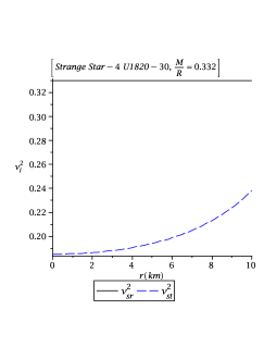
Figure 6: Variation of radial and transverse sound speed of Strange star candidate $4U~{}1820-30$

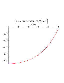
Figure 7: Variation of $v_{st}^{2}-v_{sr}^{2}$ of Strange star candidate $4U~{}1820-30$

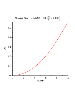
Figure 8: Variation of surface redshift of Strange star candidate $4U~{}1820-30$

3.6 Surface Redshift

The compactness of the star is given by

$$u=\frac{M}{b}=-\frac{(A+B)}{4b(m+1)A^{\frac{5}{2}}}\left[2be^{-Ab^{2}}A^{\frac{3}{2}}+\sqrt{\pi}~{}erf(\sqrt{A}b)A\right].$$ (26)

The surface redshift ($Z_{s}$) corresponding to the above compactness ($u$) is obtained as

$$1+Z_{s}=[1-2u]^{-\frac{1}{2}},$$ (27)

where,

$$1+Z_{s}=\left[1+\frac{(A+B)}{2b(m+1)A^{\frac{5}{2}}}\left(2be^{-Ab^{2}}A^{\frac{3}{2}}+\sqrt{\pi}~{}erf(\sqrt{A}b)A\right)\right]^{-\frac{1}{2}}.$$

Thus, the maximum surface redshift for a Compact Star $4U~{}1820-30$ of radius $10$ km turns out to be $Z_{s}=0.022$ (see Fig. 8).

4 Concluding Remarks

In the present work we have performed some investigations regarding the nature of compact stars after considering the following three inputs:

(1) The stars are anisotropic in their configurations, so that $p_{r}\neq p_{t}$.

(2) The erstwhile cosmological constant, introduced by Einstein, is variable in it’s character, such that $\Lambda~{}=~{}\Lambda(r)~{}=~{}\Lambda_{r}$. This assumption of variable $\Lambda$ is the outcome of the present day accelerating Universe in the form of so-called dark energy.

(3) The space-time of the interior of the compact stars can be described by KB metric.

In the investigations we have observed some interesting points which are as follows:

(i) Like normal matter distribution, the bound on the effective EOS in this construction can be given by $0<\omega_{i}(r)<1$, despite of the fact that star is constituted by the combination of ordinary matter and effect of $\Lambda$.

(ii) As one of the dark enegry candidates the cosmological variable $\Lambda$ contributes to the hydrostatic force for stability of the compact stars. However, in this connection we realize that from the point of view of the physical interpretation it would be better to consider the dark energy as being represented by a scalar field, which would lead to the interpretation of $\Lambda(r)$ as (also) being an effective description of a bosonic condensate inside the star. Literature survey shows that Boson stars or Bose-Einstein condensate stars have been intensively investigated by several investigators [27, 28, 29]. So, there is a scope to find out the possible connections between our model and the description of Boson stars. Condensates as discussed by Chavanis and Harko [27] have maximum masses of the order of $2~{}M_{sun}$, maximum central density of the order of $(0.1-0.3)x10^{16}~{}g/cm^{3}$ and minimum radii in the range of $10-20$ km are comparable to the parameters in our model-based some of the candidates of Strange Quark Star as shown in the Table-1.

(iii) By applying the cracking concept of [9] stability of the model has been attained surprisingly.

(iv) The surface redshift analysis for our case shows that for the compact star like $4U~{}1820-30$ of radius $10$ km turns out to be $0.022$. In the isotropic case and in the absence of the cosmological constant it has been shown that $z\leq 2$ [3, 30, 31]. Böhmer and Harko [31] argued that for an anisotropic star in the presence of a cosmological constant the surface red shift must obey the general restriction $z\leq 5$, which is consistent with the bound $z\leq 5.211$ as obtained by Ivanov [32]. Therefore, for an anisotropic star with cosmological constant the value $z=0.022$ seems to be too low and needs further investigation.

(v) The normal pressure $p_{r}$ vanishes but tangential pressure $p_{t}$ does not vanish at the boundary $r=b$ (radius of the star). However, the normal pressure is equal to the tangential pressure at the centre of the fluid sphere.

The overall observation is that our proposed model satisfies all physical requirements as well as horizon-free and stable. The entire analysis has been performed in connection to direct comparison of some of the Strange/Quark star candidates, e.g. $Her~{}X-1$, $SAX~{}J~{}1808.4-3658(SS1)$ and $4U~{}1820-30$ which confirms validity of the present model. Thus our approach lead to a better analytical description of the Strange/Quark stars.

References

- [1] H. Abreu, H. Hernandez and L.A. Nunez, Class. Quantum Gravit. 24 (2007) 4631.
- [2] R.L. Bowers and E.P.T. Liang, Astrophys. J. 188 (1917) 657.
- [3] H.A. Buchdahl, Phys. Rev. 116 (1959) 1027.
- [4] V.V. Burdyuzha, Astronomy Reports 53 (2009) 381.
- [5] A. Chodos et al., Phys. Rev. D. 9 (1974) 3471.
- [6] I. Dymnikova, Class. Quantum. Gravit. 19 (2002) 725.
- [7] E. Egeland, Compact Star Trondheim, Norway (2007).
- [8] A. Einstein, Sitzungs. Kon. Preuss. Akad. Wiss. (1917) 142.
- [9] L. Herrera, Phys. Lett. A 165 (1997) 206.
- [10] L. Herrera and N.O. Santos, Phys. Rep. 286 (1997) 53.
- [11] K.D. Krori and J. Barua, J. Phys. A.: Math. Gen. 8 (1975) 508.
- [12] X.-D. Li, M. Dey, J. Dey and E.P.J. Van den Heeuvel, Phys. Rev. Lett. 82 (1999) 3776.
- [13] X.-D. Li, S. Ray, J. Dey, M. Dey and I. Bombaci, Astrophys. J. 527 (1999) L51.
- [14] M.K. Mak and T. Harko, Mod. Phys. Lett. A 15 (2000) 2153.
- [15] M.K. Mak and T. Harko, Proc. R. Soc. Lond. 459 (2003) 393.
- [16] M.K. Mak and T. Harko, Int. J. Mod. Phys. D. 11 (2002) 207.
- [17] M. Kalam et al., arXiv:1201.5234[gr-qc].
- [18] S. Perlmutter et al., Nat. 391 (1998) 51.
- [19] J. Ponce de León, Gen. Relativ. Gravit. 25 (1993) 1123.
- [20] F. Rahaman et al., Phys. Rev. D 82 (2010) 104055.
- [21] F. Rahaman et al., Eur. Phys. J. C 72 (2012) 2071.
- [22] F. Rahaman et al., Gen. Rel. Grav. 44 (2012) 107.
- [23] A.G. Riess et al., Astrophys. J. 607 (2004) 665.
- [24] R. Ruderman, Rev. Astr. Astrophys. 10 (1972) 427.
- [25] V.V. Usov, Phys. Rev. D. 70 (2004) 067301.
- [26] V. Varela et al., Phys. Rev. D 82 (2010) 044052.
- [27] P.-H. Chavanis and T. Harko, Phys. Rev. D 86 (2012) 064011.
- [28] B. Hartmanna, B. Kleihausb, J. Kunzb and I. Schaffer, arXiv:1205.0899[gr-qc]
- [29] S.L. Liebling and C. Palenzuel, arXiv:1202.5809[gr-qc]
- [30] N. Straumann, General Relativity and Relativistic Astrophysics (Springer Verlag, Berlin, 1984).
- [31] C. G. Böhmer and T. Harko, Class. Quantum Gravit. 23 (2006) 6479.
- [32] B. V. Ivanov, Phys. Rev. D 65 (2002) 104011.