A Euclidean Likelihood Estimator for Bivariate Tail Dependence

Abstract

The spectral measure plays a key role in the statistical modeling of multivariate extremes. Estimation of the spectral measure is a complex issue, given the need to obey a certain moment condition. We propose a Euclidean likelihood-based estimator for the spectral measure which is simple and explicitly defined, with its expression being free of Lagrange multipliers. Our estimator is shown to have the same limit distribution as the maximum empirical likelihood estimator of J. H. J. Einmahl and J. Segers, Annals of Statistics 37(5B), 2953–2989 (2009). Numerical experiments suggest an overall good performance and identical behavior to the maximum empirical likelihood estimator. We illustrate the method in an extreme temperature data analysis.

Keywords:

Bivariate extremes; Empirical likelihood; Euclidean likelihood; Spectral measure; Statistics of extremes.

1 Introduction

When modeling dependence for bivariate extremes, only an infinite-dimensional object is flexible enough to capture the ‘spectrum’ of all possible types of dependence. One of such infinite-dimensional objects is the spectral measure, describing the limit distribution of the relative size of the two components in a vector, normalized in a certain way, given that at least one of them is large; see, for instance, Kotz and Nadarajah (2000, §3) and Beirlant et al. (2004, §8–9). The normalization of the components induces a moment constraint on the spectral measure, making its estimation a nontrivial task.

In the literature, a wide range of approaches has been proposed. Kotz and Nadarajah (2000, §2–3) survey many parametric models for the spectral measure, and new models continue to be invented (Cooley et al., 2010; Boldi and Davison, 2007; Ballani and Schlather, 2011). Here we are mostly concerned with semiparametric and nonparametric approaches. Einmahl and Segers (2009) propose an enhancement of the empirical spectral measure in Einmahl et al. (2001) by enforcing the moment constraints with empirical likelihood methods. A nonparametric Bayesian method based on the censored-likelihood approach in Ledford and Tawn (1996) is proposed in Guillotte et al. (2011).

In this paper we introduce a Euclidean likelihood-based estimator related with the maximum empirical likelihood estimator of Einmahl and Segers (2009). Our estimator replaces the empirical likelihood objective function by the Euclidean distance between the barycenter of the unit simplex and the vector of probability masses of the spectral measure at the observed pseudo-angles (Owen, 1991, 2001; Crépet et al., 2009). This construction allows us to obtain an empirical likelihood-based estimator which is simple and explicitly defined. Its expression is free of Lagrange multipliers, which not only simplifies computations but also leads to a more manageable asymptotic theory. We show that the limit distribution of the empirical process associated with the maximum Euclidean likelihood estimator measure is the same as the one of the maximum empirical likelihood estimator in Einmahl and Segers (2009). Note that standard large-sample results for Euclidean likelihood methods (Xu, 1995; Lin and Zhang, 2001) cannot be applied in the context of bivariate extremes.

The paper is organized as follows. In the next section we discuss the probabilistic and geometric frameworks supporting models for bivariate extremes. In Section 3 we introduce the maximum Euclidean likelihood estimator for the spectral measure. Large-sample theory is provided in Section 4. Numerical experiments are reported in Section 5 and an illustration with extreme temperature data is given in Section 6. Proofs and some details on a smoothing procedure using Beta kernels are given in the Appendix A and B, respectively.

2 Background

Let $(X_{1},Y_{1}),(X_{2},Y_{2}),\ldots$ be independent and identically distributed bivariate random vectors with continuous marginal distributions $F_{X}$ and $F_{Y}$. For the purposes of studying extremal dependence, it is convenient to standardize the margins to the unit Pareto distribution via $X_{i}^{*}=1/\{1-F_{X}(X_{i})\}$ and $Y_{i}^{*}=1/\{1-F_{Y}(Y_{i})\}$. Observe that $X_{i}^{*}$ exceeds a threshold $t>1$ if and only if $X_{i}$ exceeds its tail quantile $F_{X}^{-1}(1-1/t)$; similarly for $Y_{i}^{*}$. The transformation to unit Pareto distribution serves to measure the magnitudes of the two components according to a common scale which is free from the actual marginal distributions.

Pickands’ representation theorem (Pickands, 1981) asserts that if the vector of rescaled, componentwise maxima

$$\bm{M}_{n}^{*}=\biggl{(}\frac{1}{n}\max_{i=1,\ldots,n}X_{i}^{*},\frac{1}{n}\max_{i=1\ldots,n}Y_{i}^{*}\biggr{)},$$

converges in distribution to a non-degenerate limit, then the limiting distribution is a bivariate extreme value distribution $G$ with unit-Fréchet margins given by

$$G(x,y)=\exp\bigg{\{}-2\int_{[0,1]}\max\left(\frac{w}{x},\frac{1-w}{y}\right)\mathrm{d}H(w)\bigg{\}},\qquad x,y>0.$$ (1)

The spectral (probability) measure $H$ is a probability distribution on $[0,1]$ that is arbitrary apart from the moment constraint

$$\int_{[0,1]}w\,\mathrm{d}H(w)=1/2,$$ (2)

induced by the marginal distributions $G(z,\infty)=G(\infty,z)=\exp(-1/z)$ for $z>0$.

The spectral measure $H$ can be interpreted as the limit distribution of the pseudo-angle $W_{i}=X_{i}^{*}/(X_{i}^{*}+Y_{i}^{*})$ given that the pseudo-radius $R_{i}=X_{i}^{*}+Y_{i}^{*}$ is large. Specifically, weak convergence of $\bm{M}_{n}^{*}$ to $G$ is equivalent to

$$\Pr[W_{i}\in\,\cdot\,\mid R_{i}>t]\xrightarrow{w}H(\,\cdot\,),\qquad t\to\infty.$$ (3)

The pseudo-angle $W_{i}$ is close to $0$ or to $1$ if one of the components $X_{i}^{*}$ or $Y_{i}^{*}$ dominates the other one, given that at least one of them is large. Conversely, the pseudo-angle $W_{i}$ will be close to $1/2$ if both components $X_{i}^{*}$ and $Y_{i}^{*}$ are of the same order of magnitude. In case of asymptotic dependence, $G(x,y)=\exp(-1/x-1/y)$, the spectral measure puts mass $1/2$ at the atoms $0$ and $1$, whereas in case of complete asymptotic dependence $G(x,y)=\exp\{-1/\min(x,y)\}$, the spectral measure $H$ reduces to a unit point mass at $1/2$.

Given a sample $(X_{1},Y_{1}),\ldots,(X_{n},Y_{n})$, we may construct proxies for the unobservable pseudo-angles $W_{i}$ by setting

$$\hat{W}_{i} =\hat{X}_{i}^{*}/(\hat{X}_{i}^{*}+\hat{Y}_{i}^{*}), \hat{R}_{i} =\hat{X}_{i}^{*}+\hat{Y}_{i}^{*},$$

where $\hat{X}_{i}^{*}=1/\{1-\hat{F}_{X}(X_{i})\}$ and $\hat{Y}_{i}^{*}=1/\{1-\hat{F}_{Y}(Y_{i})\}$ and where $\hat{F}_{X}=\hat{F}_{X,n}$ and $\hat{F}_{Y}=\hat{F}_{Y,n}$ are estimators of the marginal distribution functions $F_{X}$ and $F_{Y}$. A robust choice for $\hat{F}_{X}$ and $\hat{F}_{Y}$ is the pair of univariate empirical distribution functions, normalized by $n+1$ rather than by $n$ to avoid division by zero. In this case, $\hat{X}_{i}^{*}$ and $\hat{Y}_{i}^{*}$ are functions of the ranks.

For a high enough threshold $t=t_{n}$, the collection of angles $\{\hat{W}_{i}:i\in K\}$ with $K=K_{n}=\{i=1,\ldots,n:\hat{R}_{i}>t\}$ can be regarded as if it were a sample from the spectral measure $H$. Parametric or nonparametric inference on $H$ may then be based upon the sample $\{\hat{W}_{i}:i\in K\}$. Nevertheless, two complications occur:

1. The choice of the threshold $t$ comes into play both through the rate of convergence in (3) and through the effective size $|K|=k$ of the sample of pseudo-angles.

2. The standardization via the estimated margins induces dependence between the pseudo-angles, even when the original random vectors $(X_{i},Y_{i})$ are independent.

For the construction of estimators of the spectral measure, we may thus pretend that $\{\hat{W}_{i}:i\in I\}$ constitutes a sample from $H$. However, for the theoretical analysis of the resulting estimators, the two issues above must be taken into consideration. Failure to do so will lead to a wrong assessment of both the bias and the standard errors of estimators of extremal dependence.

3 Maximum Euclidean Likelihood Estimator

We propose to use Euclidean likelihood methods (Owen, 2001, pp. 63–66) to estimate the spectral measure. Let $w_{1},\ldots,w_{k}\in[0,1]$ be a sample of pseudo-angles, for example the observed values of the random variables $\hat{W}_{i}$, $i\in K$, in the previous section, with $k=|K|$. The Euclidean loglikelihood $\ell_{\text{E}}$ ratio for a candidate spectral measure $H$ supported on $\{w_{1},\ldots,w_{k}\}$ and assigning probability mass $p_{i}=H(\{w_{i}\})$ to $w_{i}$ is formally defined as

$$\ell_{\text{E}}(\bm{p})=-\frac{1}{2}\sum_{i=1}^{k}(kp_{i}-1)^{2}.$$

The Euclidean likelihood ratio can be viewed as a Euclidean measure of the distance of $\bm{p}=(p_{1},\ldots,p_{k})$ to the barycenter $(k^{-1},\ldots,k^{-1})$ of the $(k-1)$-dimensional unit simplex. In this sense, the Euclidean likelihood ratio is similar to the empirical loglikelihood ratio

$$\ell(\bm{p})=\sum_{i=1}^{k}\log(kp_{i}),$$

which can be understood as another measure of the distance from $\bm{p}$ to $(k^{-1},\ldots,k^{-1})$. Note that $\ell_{\text{E}}(\bm{p})$ results from $\ell(\bm{p})$ by truncation of the Taylor expension $\log(1+x)=x-x^{2}/2+\cdots$ and the fact that $p_{1}+\cdots+p_{k}=1$, making the linear term in the expansion disappear.

We seek to maximize $\ell_{\text{E}}(\bm{p})$ subject to the empirical version of the moment constraint (2). Our estimator $\hat{H}$ for the distribution function of the spectral measure is defined as

$$\hat{H}(w)=\sum_{i=1}^{k}\hat{p}_{i}\,I(w_{i}\leq w),\qquad w\in[0,1],$$ (4)

the vector of probability masses $\hat{\bm{p}}=(\hat{p}_{1},\ldots,\hat{p}_{k})$ solving the optimization problem

$$\begin{array}[]{rl}\underset{\bm{p}\in\mathbb{R}^{k}}{\max}&-\frac{1}{2}\sum_{i=1}^{k}(kp_{i}-1)^{2}\\ \text{s.t.}&\sum_{i=1}^{k}p_{i}=1\\ &\sum_{i=1}^{k}w_{i}p_{i}=1/2.\end{array}$$ (5)

This quadratic program with linear constraints can be solved explicitly with the method of Lagrange multipliers, yielding

$$\hat{p}_{i}=\frac{1}{k}\bigl{\{}1-(\overline{w}-1/2)S^{-2}(w_{i}-\overline{w})\bigr{\}},\qquad i=1,\ldots,k,$$ (6)

where $\overline{w}$ and $S^{2}$ denote the sample mean and sample variance of $w_{1},\ldots,w_{k}$, that is,

$$\overline{w} =\frac{1}{k}\sum_{i=1}^{k}w_{i}, S^{2} =\frac{1}{k}\sum_{i=1}^{k}(w_{i}-\overline{w})^{2}.$$

The weights $\hat{p}_{i}$ could be negative, but our numerical experiments suggest that this is not as problematic as it may seem at first sight, in agreement with Antoine et al. (2007) and Crépet et al. (2009), who claim that the weights $p_{i}$ are nonnegative with probability tending to one. The second equality constraint in (5) implies that $\hat{H}$ satisfies the moment constraint (2), as $\int_{[0,1]}w\,\mathrm{d}\hat{H}(w)=\sum_{i}w_{i}\hat{p}_{i}=1/2$, which can be easily verified directly.

The empirical spectral measure estimator of Einmahl et al. (2001) and the maximum empirical likelihood estimator of Einmahl and Segers (2009) can be constructed as in (5) through suitable changes in the objective function and the constraints. The empirical spectral measure $\dot{H}(w)=\sum_{i}\dot{p}_{i}\,I(w_{i}\leq w)$ solves the optimization problem

$$\begin{array}[]{rl}\underset{\bm{p}\in\mathbb{R}^{k}_{+}}{\max}&\sum_{i=1}^{k}\log p_{i}\\ \mbox{s.t.}&\sum_{i=1}^{k}p_{i}=1.\end{array}$$

yielding $\dot{p}_{i}=1/k$ for $i=1,\ldots,k$. In contrast, the maximum empirical likelihood estimator $\ddot{H}(w)=\sum_{i}\ddot{p}_{i}\,I(w_{i}\leq w)$ has probability masses given by the solution of

$$\begin{array}[]{rl}\underset{\bm{p}\in\mathbb{R}^{k}_{+}}{\max}&\sum_{i=1}^{k}\log p_{i}\\ \mbox{s.t.}&\sum_{i=1}^{k}p_{i}=1\\ &\sum_{i=1}^{k}w_{i}p_{i}=1/2.\end{array}$$ (7)

By the method of Lagrange multipliers, the solution is given by

$$\ddot{p}_{i}=\frac{1}{k}\frac{1}{1+\lambda(w_{i}-1/2)},\qquad i=1,\ldots,k,$$

where $\lambda\in\mathbb{R}$ is the Lagrange multiplier associated to the second equality constraint in (7), defined implicitly as the solution to the equation

$$\frac{1}{k}\sum_{i=1}^{k}\frac{w_{i}-1/2}{{1+\lambda(w_{i}-1/2)}}=0,$$

see also Qin and Lawless (1994).

4 Large-Sample Theory

The maximum Euclidean likelihood estimator $\hat{H}$ in (4) can be expressed in terms of the empirical spectral measure $\dot{H}$ given by

$$\dot{H}(w)=\frac{1}{k}\sum_{i=1}^{k}I(w_{i}\leq w),\qquad w\in[0,1].$$

Indeed, $\overline{w}$ and $S^{2}$ are just the mean and the variance of $\dot{H}$, and the expression (6) for the weights $\hat{p}_{i}$ can be written as

$$\frac{\mathrm{d}\hat{H}}{\mathrm{d}\dot{H}}(v)=1-(\overline{w}-1/2)\,S^{-2}\,(v-\overline{w}),\qquad v\in[0,1].$$

Integrating out this ‘likelihood ratio’ over $v\in[0,w]$ yields the identity

$$\hat{H}(w)=(\Phi(\dot{H}))(w),\qquad w\in[0,1],$$

where the transformation $\Phi$ is defined as follows. Let $\mathbb{D}_{\Phi}$ be the set of cumulative distribution functions of non-degenerate probability measures on $[0,1]$. For $F\in\mathbb{D}_{\Phi}$, the function $\Phi(F)$ on $[0,1]$ is defined by

$$(\Phi(F))(w)=F(w)-(\mu_{F}-1/2)\,\sigma_{F}^{-2}\,\int_{[0,w]}(v-\mu_{F})\,\mathrm{d}F(v),\qquad w\in[0,1].$$

Here $\mu_{F}=\int_{[0,1]}v\,\mathrm{d}F(v)$ and $\sigma_{F}^{2}=\int_{[0,1]}(v-\mu_{F})^{2}\,\mathrm{d}F(v)$ denote the mean and the (non-zero) variance of $F$.

We view $\mathbb{D}_{\Phi}$ as a subset of the Banach space $\ell^{\infty}([0,1])$ of bounded, real-valued functions on $[0,1]$ equipped with the supremum norm $\|\,\cdot\,\|_{\infty}$. The map $\Phi$ takes values in $\ell^{\infty}([0,1])$ as well. Weak convergence in $\ell^{\infty}([0,1])$ is denoted by the arrow ‘$\rightsquigarrow$’ and is to be understood as in van der Vaart and Wellner (1996).

Asymptotic properties of the empirical spectral measure together with smoothness properties of $\Phi$ lead to asymptotic properties of the maximum Euclidean likelihood estimator:

• Continuity of the map $\Phi$ together with consistency of the empirical spectral measure yields consistency of the maximum Euclidean likelihood estimator (continuous mapping theorem).

• Hadamard differentiability of the map $\Phi$ together with asymptotic normality of the empirical spectral measure yields asymptotic normality of the maximum Euclidean likelihood estimator (functional delta method).

The following theorems are formulated in terms of maps $\dot{H}_{n}$ taking values in $\mathbb{D}_{\Phi}$. The case to have in mind is the empirical spectral measure $\dot{H}_{n}(w)=k_{n}^{-1}\sum_{i\in K_{n}}I(\hat{W}_{i}\leq w)$ with $\{\hat{W}_{i}:i\in K_{n}\}$ and $k_{n}=|K_{n}|$ as in Section 2. In Theorem 3.1 and equation (7.1) of Einmahl and Segers (2009), asymptotic normality of $\dot{H}_{n}$ is established under certain smoothness conditions on $H$ and growth conditions on the threshold sequence $t_{n}$.

Theorem 1 (Consistency).

If $\dot{H}_{n}$ are maps taking values in $\mathbb{D}_{\Phi}$ and if $\|\dot{H}_{n}-H\|_{\infty}\to 0$ in outer probability for some nondegenerate spectral measure $H$, then, writing $\hat{H}_{n}=\Phi(\dot{H}_{n})$, we also have $\|\hat{H}_{n}-H\|_{\infty}\to 0$ in outer probability.

The proof of this and the next theorem is given in Appendix A. In the next theorem, the rate sequence $r_{n}$ is to be thought of as $\sqrt{k_{n}}$. Let $\mathcal{C}([0,1])$ be the space of continuous, real-valued functions on $[0,1]$.

Theorem 2 (Asymptotic normality).

Let $\dot{H}_{n}$ and $H$ be as in Theorem 1. If $H$ is continuous and if

$$r_{n}(\dot{H}_{n}-H)\rightsquigarrow\beta,\qquad n\to\infty,$$

in $\ell^{\infty}([0,1])$, with $0<r_{n}\to\infty$ and with $\beta$ a random element of $\mathcal{C}([0,1])$, then also

$$r_{n}(\hat{H}_{n}-H)\rightsquigarrow\gamma,\qquad n\to\infty$$

with

$$\gamma(w)=\beta(w)-\sigma_{H}^{-2}\,\int_{0}^{1}\beta(v)\,\mathrm{d}v\,\int_{0}^{w}(1/2-v)\,\mathrm{d}H(v),\qquad w\in[0,1].$$ (8)

Comparing the expression for $\gamma$ in (8) with the one for $\gamma$ in (4.7) in Einmahl and Segers (2009), we see that the link between the processes $\beta$ and $\gamma$ here is the same as the one between the processes $\beta$ and $\gamma$ in Einmahl and Segers (2009). It follows that tuning the empirical spectral measure via either maximum empirical likelihood or maximum Euclidean likelihood makes no difference asymptotically. The numerical experiments below confirm this asymptotic equivalence. To facilitate comparisons with Einmahl and Segers (2009), note that our pseudo-angle $w\in[0,1]$ is related to their radial angle $\theta\in[0,\pi/2]$ via $\theta=\arctan\{w/(1-w)\}$, and that the function $f$ in (4.2) in Einmahl and Segers (2009) reduces to $f(\theta)=(\sin\theta-\cos\theta)/(\sin\theta+\cos\theta)=2w-1$.

How does the additional term $\sigma_{H}^{-2}\,\int_{0}^{1}\beta(v)\,\mathrm{d}v\,\int_{0}^{w}(1/2-v)\,\mathrm{d}H(v)$ influence the asymptotic distribution of the maximum Euclidean/empirical estimator? Given the complicated nature of the covariance function of the process $\beta$, see (3.7) and (4.7) in Einmahl and Segers (2009), it is virtually impossible to draw any conclusions theoretically. However, Monte Carlo simulations in Einmahl and Segers (2009, §5.1) confirm that the maximum empirical likelihood estimator is typically more efficient than the ordinary empirical spectral measure. These findings are confirmed in the next section.

5 Monte Carlo Simulations

In this section, the maximum Euclidean likelihood estimator is compared with the empirical spectral measure and the maximum empirical likelihood estimator by means of Monte Carlo simulations. The comparisons are made on the basis of the mean integrated squared error,

$$\text{MISE($\cdot$)}=E\bigg{[}\int_{0}^{1}\{\cdot-H(w)\}^{2}\mathrm{d}w\bigg{]}.$$

The bivariate extreme value distribution $G$ with logistic dependence structure is defined by

$$G(x,y)=\exp\{-(x^{-1/\alpha}+y^{-1/\alpha})^{\alpha}\},\qquad x,y>0,$$

in terms of a parameter $\alpha\in(0,1]$. Smaller values of $\alpha$ yield stronger dependence and the limiting cases $\alpha\to 0$ and $\alpha=1$ correspond to complete dependence and exact independence, respectively. For $0<\alpha<1$, the spectral measure $H_{\alpha}$ is absolutely continuous with density

$$\frac{\mathrm{d}H_{\alpha}(w)}{\mathrm{d}w}=\frac{1}{2}(\alpha^{-1}-1)\{w(1-w)\}^{-1-1/\alpha}\big{\{}w^{-1/\alpha}+(1-w)^{-1/\alpha}\big{\}}^{\alpha-2},\qquad 0<w<1.$$

Here we consider $\alpha_{\textsc{i}}=0.8$ and $\alpha_{\textsc{ii}}=0.4$, with stronger extremal dependence corresponding to case ii. For each of these two models, 1000 Monte Carlo samples of size 1000 were generated. The thresholds were set at the empirical quantiles of the radius $\widehat{R}$ given by $t=75\%,75.5\%,\ldots,99.5\%$ for case i and $t=50\%,50.5\%,\ldots,99.5\%$ for case ii. The margins were estimated parametrically, by fitting univariate extreme value distributions using maximum likelihood.

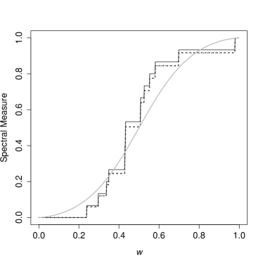
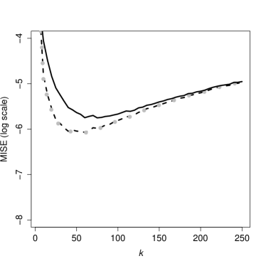
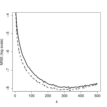
In Figure 1, a typical trajectory of the estimators is shown, illustrating the closeness of the maximum Euclidean and empirical likelihood estimators. The good performance of the maximum Euclidean/empirical spectral measure is confirmed by Figure 2. For larger $k$ (lower threshold $t$), the bias coming from the approximation error in (3) is clearly visible.

Figure 1: Examples of trajectories of the empirical spectral measure (solid), the maximum empirical likelihood estimator (dashed), and the maximum Euclidean likelihood estimator (dotted). The solid grey line corresponds to the true spectral measure $H_{\alpha}$ coming from the bivariate logistic extreme value distribution with parameters $\alpha_{\textsc{i}}=0.8$ (left) and $\alpha_{\textsc{ii}}=0.4$ (right).

Figure 2: Logarithms of the mean integrated squared errors of the spectral measure estimates based on 1000 samples of size 1000 from the bivariate logistic extreme value distribution with parameters $\alpha_{\textsc{i}}=0.8$ (left) and $\alpha_{\textsc{ii}}=0.4$ (right). The solid, dashed, and dotted lines correspond to the empirical spectral measure, the maximum empirical likelihood estimator, and the maximum Euclidean likelihood estimator, respectively.

Numerical experiments in Einmahl and Segers (2009, §5.2) show that the presence of atoms at the endpoints $0$ and $1$ has an adverse effect on maximum Euclidean/empirical likelihood estimates, and this finding is further confirmed by Guillotte et al. (2011, §7.1). Indeed, by construction, the pseudo-angles $\hat{W}_{i}$ will never be exactly $0$ or $1$. The empirical spectral measure therefore does not assign any mass at $0$ and $1$, and this situation cannot be remedied by the maximum empirical or Euclidean likelihood estimators, having the same support as the empirical spectral measure.

The weights $\hat{p}_{i}$ of the maximum Euclidean likelihood estimator can be negative. However, as can be seen from Figure 3, the weights tend to be positive overall, except for extremely high thresholds, with the proportion of negative weights being smaller in case i. This suggests that the closer we get to exact independence, the lower the proportion of negative weights.

Figure 3: Proportion of negative weights based on 1000 samples of size 1000 from the bivariate logistic extreme value distribution with parameters $\alpha_{\textsc{i}}=0.8$ (left) and $\alpha_{\textsc{ii}}=0.4$ (right).

6 Extreme Temperature Data Analysis

6.1 Data Description and Preliminary Considerations

The data were gathered from the Long-term Forest Ecosystem Research database, which is maintained by LWF (Langfristige Waldökosystem-Forschung), and consist of daily average meteorological measurements made in Beatenberg’s forest in the canton of Bern, Switzerland. More information on these data can be found at

http://www.wsl.ch

and for an extensive study see Ferrez et al. (2011). Two time series of air temperature data are available: One in the open field and the other in a nearby site under the forest cover. Our aim is to understand how the extremes in the open relate with those under the canopy; comparison of open-site and below-canopy climatic conditions is a subject of considerable interest in Forestry and Meteorology Renaud and Rebetez (2009); Ferrez et al. (2011); Renaud et al. (2011). The raw data are plotted in Figure 4, but before we are able to measure extremal dependence of open air and forest cover temperatures we first need to preprocess the data. The preprocessing step is the same as in Ferrez et al. (2011, §3.1) and further details can be found in there.

Figure 4: Daily average air temperatures from the meteorological station in Beatenberg’s forest: under the forest cover (left) and in the open field (right).

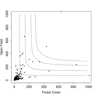
We consider daily maxima of the residual series that result from removal of the annual cycle in both location and scale, and we then take the residuals at their 98% quantile; hence the threshold boundary is defined as $U=\{(x,y)\in[0,\infty)^{2}:x+y=\widehat{F}^{-1}_{\widehat{R}}(0.98)=105.83\}$, so that there are $|U|=k=57$ exceedances.

Figure 5: Scatterplot of air temperature data after transformation to unit Fréchet scale; the solid line corresponds to the boundary threshold in the log-log scale, with both axes being logarithmic.

Figure 6: Empirical estimates and 95% pointwise confidence intervals for $\chi(u)$ (left) and $\overline{\chi}(u)$ (right) as a function of $u\in(0,1)$.

The dependence between open field and forest cover temperatures can be observed in Figure 5, where we plot a log-log scale scatterplot of the unit Fréchet data, and where we note that after log transformation the linearity of the threshold boundary $U$ is perturbed.

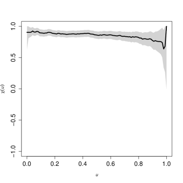
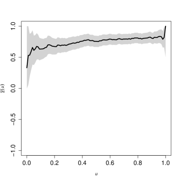
Spectral measures are only appropriate for modeling asymptotically dependent data. Although this issue has been already addressed in Ferrez et al. (2011), for exploratory purposes we present in Figure 6 the empirical estimates of the dependence coefficients $\chi(u)$ and $\overline{\chi}(u)$, for $0<u<1$, defined in Coles et al. (1999) as

$$\chi(u) =2-\log\frac{\Pr[F_{X}(X)<u,F_{Y}(Y)<u]}{\log\Pr[F_{X}(X)<u]}, \overline{\chi}(u) =\frac{2\log(1-u)}{\log\Pr[F_{X}(X)>u,F_{Y}(Y)>u]}-1.$$

Although these plots fail to have a clear-cut interpretation given the large uncertainty entailed in the estimation, the point estimates seem to be consistent with asymptotic dependence as already noticed by Ferrez et al. (2011).

6.2 Extremal Dependence of Open Air and Forest Cover Temperatures

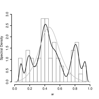
We now apply the maximum Euclidean likelihood estimator to measure extremal dependence of open air and forest cover temperatures. The estimated spectral measure is shown in Figure 7. All weights are positive, i.e. $\hat{p}_{i}>0$, for $i=1,\ldots,57$.

By construction, the estimate of the spectral measure is discrete. A smooth version which still obeys the moment constraint (2) can easily obtained by smoothing the maximum Euclidean or empirical likelihood estimator with a Beta kernel. Related ideas are already explored in Hall and Presnell (1999) and Chen (1997). Details are given in Appendix B.

A cross-validatory procedure was used to select the bandwidth, yielding a concentration parameter of $\nu\approx 163$. Numerical experiments in Warchoł (2012) suggest that convoluting empirical likelihood-based estimators with a Beta kernel yields a further reduction in mean integrated squared error. The Beta kernel even outperforms Chen’s kernel (Chen, 1999), which is asymptotically optimal under some conditions (Bouezmarni and Rolin, 2003), but which is unable to conserve the moment constraint.

From the smoothed spectral measure, we obtain an estimate of the spectral density and plug-in estimators for the Pickands dependence function $A(w)=1-w+2\int_{0}^{w}H(v)\,\mathrm{d}v$, $w\in[0,1]$, and the bivariate extreme value distribution in (1). The estimated spectral density is compared with the fit obtained from the asymmetric logistic model

$$H_{\alpha,\psi_{1},\psi_{2}}(w)=\frac{1}{2}\bigg{[}1+\psi_{1}+\psi_{2}-\{\psi_{1}^{1/\alpha}(1-w)^{1/\alpha-1}-\psi_{2}^{r}w^{1/\alpha-1}\}\\ \{\psi_{1}^{1/\alpha}(1-w)^{1/\alpha}+\psi_{2}^{1/\alpha}w^{1/\alpha}\}^{1/1/\alpha-1}\bigg{]},\qquad w\in[0,1],$$

with parameter estimates $\widehat{\psi}_{1}=0.78$ (standard error $0.03$), $\widehat{\psi}_{2}=0.90$ ($0.03$) and $\widehat{\alpha}=0.30$ ($0.02$). The asymmetric logistic model was considered by Ferrez et al. (2011) as the parametric model that achieved the “best overall fit.”

In Figure 7 we also plot the smooth spectral measure and corresponding spectral density which are obtained by suitably convoluting the empirical Euclidean spectral measure with a Beta kernel as described in (9) and (10). Since more mass concentrated over 1/2 corresponds to more extremal dependence, and more mass concentrated on 0 and 1 corresponds more independence in the extremes, a rough interpretation for our context is as follows: The lower the shelter ability of the forest, the more mass should be concentrated around 1/2, whereas higher shelter ability corresponds to the case where the spectral measure gets more mass concentrated at 1; more mass concentrated at 0 suggests relatively more extreme events under the forest cover, suggesting that the forest has the ability to retain heat during extreme events.

Figure 7: Estimates of the spectral measure (left) and the spectral density (right). Left: the dotted line corresponds to the empirical Euclidean spectral measure, and the solid line corresponds to its smooth version constructed using (10). Right: The solid line corresponds to the smooth spectral density obtained from the Euclidean likelihood weights using (9), and the gray line represents the fit from the asymmetric logistic model with $(\widehat{\psi}_{1},\widehat{\psi}_{2})=(0.78,0.90)$ and $\widehat{\rho}=0.30$.

In Figure 8.1 we plot the corresponding Pickands dependence function. More extremal dependence corresponds to lower Pickands dependence functions, and the deeper these are on the right the less frequent are the extreme events under the forest cover relatively to the open field. Our analysis suggests that extreme high temperatures under the forest cover are more frequent than expected from a corresponding parametric analysis. This somewhat surprising finding is already predicted in Ferrez et al. (2011, Fig. 4). The phenomenon may be due to the ability of some forests to retain heat, acting like a greenhouse, or it may be connected with the way that other features of the forest’s structure can alter its microclimate (Renaud et al., 2011). Along with the Pickands dependence function, we also plot in Figure 8.1 the pseudo-angles which provide further evidence of a marked right skewness.

The joint behavior of temperatures in the open and under forest cover can also be examined from the estimated bivariate extreme value distribution function plotted in Figure 8.2, which was constructed by convoluting the empirical Euclidean spectral measure with a Beta kernel as described in (13).

Figure 8: Estimates of the Pickands dependence function and contours of the bivariate extreme value distribution. Left: The solid line represents the smooth Pickands dependence function obtained from the Euclidean likelihood weights using (12), and the gray line represents the fit from the asymmetric logistic model with $(\widehat{\psi}_{1},\widehat{\psi}_{2})=(0.78,0.90)$ and $\widehat{\rho}=0.30$. The pseudo-angles are presented at the top. Right: The solid gray line represents the smooth bivariate extreme value distribution obtained from the Euclidean likelihood weights using (13). Air temperature data are plotted on the unit Fréchet scale.

7 Discussion

In this paper we propose a simple empirical likelihood-based estimator for the spectral measure, whose asymptotic efficiency is comparable to the empirical likelihood spectral measure of Einmahl and Segers (2009). The fact that our estimator has the same limit distribution as the empirical likelihood spectral measure, suggests that a more general result may hold for other members of the Cressie–Read class, of which these estimators are particular cases, similarly to what was established by Baggerly (1998) in a context different from ours. We focus on the spectral measure defined over the $L_{1}$-norm, but only for a matter of simplicity, and there is no problem in defining our estimator for the spectral measure defined over the $L_{p}$-norm, with $p\in[1,\infty]$. For real data applications smooth versions of empirical the estimator may be preferred, but these can be readily constructed by suitably convoluting the weights of our empirical likelihood-based method with a kernel on the simplex.

Appendix A Proofs

Proof of Theorem 1.

Let $F_{n},F\in\mathbb{D}_{\Phi}$. By Fubini’s theorem,

$$\int_{[0,w]}v\,\mathrm{d}F(v) =w\,F(w)-\int_{0}^{w}F(v)\,\mathrm{d}v,\qquad w\in[0,1],$$

$$\int_{[0,1]}v^{2}\,\mathrm{d}F(v) =1-\int_{0}^{1}2v\,F(v)\,\mathrm{d}v,$$

and similarly for $F_{n}$. It follows that $\|F_{n}-F\|_{\infty}\to 0$ implies that $\mu_{F_{n}}\to\mu_{F}$, $\sigma_{F_{n}}^{2}\to\sigma_{F}^{2}$, and $\int_{[0,w]}v\,\mathrm{d}F_{n}(v)\to\int_{[0,w]}v\,\mathrm{d}F(v)$ uniformly in $w\in[0,1]$. Hence $\|\Phi(F_{n})-\Phi(F)\|_{\infty}\to 0$. Therefore, the map $\Phi:\mathbb{D}_{\Phi}\to\ell^{\infty}([0,1])$ is continuous. The lemma now follows from the fact that $\Phi(H)=H$ together with the continuous mapping theorem, see Theorem 1.9.5 in van der Vaart and Wellner (1996). ∎

Proof of Theorem 2.

Write

$$\beta_{n} =r_{n}(\dot{H}_{n}-H), \gamma_{n} =r_{n}(\hat{H}_{n}-H).$$

Let $\mathbb{D}_{n}$ denote the set of functions $f\in\ell^{\infty}([0,1])$ such that $H+r_{n}^{-1}f$ belongs to $\mathbb{D}_{\Phi}$. Since $H+r_{n}^{-1}\beta_{n}=\dot{H}_{n}$ takes values in $\mathbb{D}_{\Phi}$, it follows that $\beta_{n}$ takes values in $\mathbb{D}_{n}$. Define $g_{n}:\mathbb{D}_{n}\to\ell^{\infty}([0,1])$ by

$$g_{n}(f)=r_{n}\{\Phi(H+r_{n}^{-1}f)-H\}.$$

Observe that

$$g_{n}(\beta_{n})=r_{n}\{\Phi(\dot{H}_{n})-H\}=\gamma_{n}.$$

Further, define the map $g:\mathcal{C}([0,1])\to\mathcal{C}([0,1])$ by

$$(g(f))(w)=f(w)-\sigma_{H}^{-2}\,\int_{0}^{1}f(v)\,\mathrm{d}v\,\int_{0}^{w}(1/2-v)\,\mathrm{d}H(v),\qquad w\in[0,1].$$

A straightforward computation shows that if $f_{n}\in\mathbb{D}_{n}$ is such that $\|f_{n}-f\|_{\infty}\to 0$ for some $f\in\mathcal{C}([0,1])$, then $\|g_{n}(f_{n})-g(f)\|_{\infty}\to 0$; note in particular that $f_{n}(1)=0$ and thus also $f(1)=0$. The extended continuous mapping theorem (van der Vaart and Wellner, 1996, Theorem 1.11.1) implies that

$$\gamma_{n}=g_{n}(\beta_{n})\to g(\beta)=\gamma,\qquad n\to\infty,$$

as required. Note that we have actually shown that $\Phi$ is Hadamard differentiable at $H$ tangentially to $\mathcal{C}([0,1])$ with derivative given by $\Phi_{F}^{\prime}=g$. The result then also follows from the functional delta method. ∎

Appendix B Beta-Kernel Smoothing of Discrete Spectral Measures

We only consider the case of the empirical Euclidean spectral measure using a Beta kernel, but the same applies to the empirical likelihood spectral measure by replacing the $\widehat{p_{i}}$ with $\ddot{p}_{i}$ in (3). The smooth Euclidean spectral density is thus defined as

$$\widetilde{h}(w)=\sum_{i=1}^{k}\widehat{p}_{i}\,\beta\{w;w_{i}\nu,(1-w_{i})\nu\},\qquad w\in(0,1),$$ (9)

where $\nu>0$ is the concentration parameter (inverse of the squared bandwidth, to be chosen via cross-validation) and $\beta(w;p,q)$ denotes the Beta density with parameters $p,q>0$. The corresponding smoothed spectral measure is defined as

$$\widetilde{H}(w)=\int_{0}^{w}\widetilde{h}(v)\,\mathrm{d}v=\sum_{i=1}^{k}\widehat{p}_{i}\mathcal{B}\{w;w_{i}\nu,(1-w_{i})\nu\},\qquad w\in[0,1],$$ (10)

where $\mathcal{B}(w;p,q)$ is the regularized incomplete beta function, with $p,q>0$. Since

$$\int_{0}^{1}w\,\widetilde{h}(w)\,\mathrm{d}w=\sum_{i=1}^{k}\widehat{p}_{i}\bigg{\{}\frac{\nu w_{i}}{\nu w_{i}+\nu(1-w_{i})}\bigg{\}}=\sum_{i=1}^{k}\widehat{p}_{i}w_{i}=1/2,$$ (11)

the moment constraint is satisfied. Plug-in estimators for the Pickands dependence function and the bivariate extreme value distribution follow directly from

$$\widetilde{A}(w) =1-w+2\sum_{i=1}^{k}\widehat{p}_{i}\int_{0}^{w}\mathcal{B}\{u;w_{i}\nu,(1-w_{i})\nu\}\mathrm{d}u,\qquad w\in[0,1],$$ (12)

$$\widetilde{G}(x,y) =\exp\left\{-\frac{2}{k}\sum_{i=1}^{k}\widehat{p}_{i}\int_{0}^{1}\max\bigg{(}\frac{u}{x},\frac{1-u}{y}\bigg{)}\beta\{u;w_{i}\nu,(1-w_{i})\nu\}\mathrm{d}u\right\},\qquad x,y>0.$$ (13)

References

- Antoine et al. (2007) Antoine, B., Bonnal, H., Renault, E. (2007). On the efficient use of the informational content of estimating equations: Implied probabilities and Euclidean empirical likelihood. J. Econometrics 138(2): 461–487.
- Baggerly (1998) Baggerly, K. A. (1998). Empirical likelihood as a goodness-of-fit measure. Biometrika 85(3): 535–547.
- Ballani and Schlather (2011) Ballani, F., Schlather, M. (2011). A construction principle for multivariate extreme value distributions. Biometrika 98(3): 633–645.
- Beirlant et al. (2004) Beirlant, J., Goegebeur, Y., Segers, J., Teugels, J. (2004). Statistics of Extremes: Theory and Applications. New York: Wiley.
- Boldi and Davison (2007) Boldi, M.-O., Davison, A. C. (2007). A mixture model for multivariate extremes. J. R. Statist. Soc. B 69(2): 217–229.
- Bouezmarni and Rolin (2003) Bouezmarni, T., Rolin, J.-M. (2003). Consistency of the beta kernel density function estimator. Canadian J. Statist. 31(1): 89–98.
- Chen (1997) Chen, S. X. (1997). Empirical likelihood-based kernel density estimation. Austral. J. Statist 39(1): 47–56.
- Chen (1999) Chen, S. X. (1999). Beta kernel estimators for density functions. Comput. Statist. Data Anal. 31(2): 131–145.
- Coles et al. (1999) Coles, S. G., Heffernan, J., Tawn, J. A. (1999). Dependence measures for extreme value analyses. Extremes 2(4): 339–365.
- Cooley et al. (2010) Cooley, D., Davis, R. A., Naveau, P. (2010). The pairwise beta distribution: A flexible parametric multivariate model for extremes. J. Mult. Anal. 101(9): 2103–2117.
- Crépet et al. (2009) Crépet, A., Harari-Kermadec, H., Tressou, J. (2009). Using empirical likelihood to combine data: Application to food risk assessment. Biometrics 65(1): 257–266.
- Einmahl et al. (2001) Einmahl, J. H. J., de Haan, L., Piterbarg, V. I. (2001). Nonparametric estimation of the spectral measure of an extreme value distribution. Ann. Statist. 29(5): 1401–1423.
- Einmahl and Segers (2009) Einmahl, J. H. J., Segers, J. (2009). Maximum empirical likelihood estimation of the spectral measure of an extreme-value distribution. Ann. Statist. 37(5B): 2953–2989.
- Ferrez et al. (2011) Ferrez, J. F., Davison, A. C., Rebetez, M. (2011). Extreme temperature analysis under forest cover compared to an open field. Agric. Forest Meteo. 151(7): 992–1001.
- Guillotte et al. (2011) Guillotte, S., Perron, F., Segers, J. (2011). Non-parametric Bayesian inference on bivariate extremes. J. R. Statist. Soc. B 73(3): 377–406.
- Hall and Presnell (1999) Hall, P., Presnell, B. (1999). Density estimation under constraints. J. Comput. Graph. Statist. 8(2): 259–277.
- Kotz and Nadarajah (2000) Kotz, S., Nadarajah, S. (2000). Extreme Value Distributions: Theory and Applications. London: Imperial College Press.
- Ledford and Tawn (1996) Ledford, A. W., Tawn, J. A. (1996). Statistics for near independence in multivariate extreme values. Biometrika 83(1): 169–187.
- Lin and Zhang (2001) Lin, L., Zhang, R. (2001). Blockwise empirical Euclidean likelihood for weakly dependent processes. Statist. Prob. Lett. 53(2): 143–152.
- Owen (1991) Owen, A. B. (1991). Empirical likelihood for linear models. Ann. Statist. 19(4): 1725–1747.
- Owen (2001) Owen, A. B. (2001). Empirical Likelihood. Boca Raton: Chapman and Hall.
- Pickands (1981) Pickands, J., I. (1981). Multivariate extreme value distributions. Bulletin Int. Statist. Inst., Proc. 43rd Sess. (Buenos Aires), pp. 859–878. Voorburg, Netherlands: ISI.
- Qin and Lawless (1994) Qin, J., Lawless, J. (1994). Empirical likelihood and general estimating equations. Ann. Statist. 22(1): 300–325.
- Renaud et al. (2011) Renaud, V., Innes, J. L., Dobbertin, M., Rebetez, M. (2011). Comparison between open-site and below-canopy climatic conditions in Switzerland for different types of forests over 10 years (1998–2007). Theor. Appl. Climatol. 105(1–2): 119–127.
- Renaud and Rebetez (2009) Renaud, V., Rebetez, M. (2009). Comparison between open-site and below-canopy climatic conditions in Switzerland during the exceptionally hot summer of 2003. Agric. Forest Meteo. 149: 873–880.
- van der Vaart and Wellner (1996) Van der Vaart, A. W., Wellner, J. A. (1996). Weak Convergence and Empirical Processes: With Applications to Statistics. New York: Springer.
- Warchoł (2012) Warchoł, M. (2012). Smoothing Methods for Bivariate Extremes. Joint MSc thesis, Ecole Polytechnique Fédérale de Lausanne and Uniwersytet Jagielloński.
- Xu (1995) Xu, L. (1995). Large sample properties of the empirical Euclidean likelihood estimation for semiparametric model. Chinese J. Appl. Prob. Statist. 10: 344–352.