Optimizing Scrip Systems: Crashes, Altruists, Hoarders, Sybils and Collusion

Abstract

Scrip, or artificial currency, is a useful tool for designing systems that are robust to selfish behavior by users. However, it also introduces problems for a system designer, such as how the amount of money in the system should be set. In this paper, the effect of varying the total amount of money in a scrip system on efficiency (i.e., social welfare—the total utility of all the agents in the system) is analyzed, and it is shown that by maintaining the appropriate ratio between the total amount of money and the number of agents, efficiency is maximized. This ratio can be found by increasing the money supply to just below the point that the system would experience a “monetary crash,” where money is sufficiently devalued that no agent is willing to perform a service. The implications of the presence of altruists, hoarders, sybils, and collusion on the performance of the system are examined. Approaches are discussed to identify the strategies and types of agents.

1 Introduction

Money is a powerful tool for dealing with selfish behavior. For example, in peer-to-peer systems, a common problem is free riding Adar and Huberman (2000), where users take advantage of the resources offered by a system without contributing their own. One way of dealing with the problem is to have users pay for the use of others’ resources, and to pay them for contributing their own resources. The incentive to free ride then disappears. Similarly, monetary incentives are a potential solution to resource allocation problems in distributed and peer-to-peer systems: this is the business model of cloud computing services such as Amazon EC2.

In some systems, it may not be desirable to use actual money. As a result, many systems have used an artificial currency, or scrip. (See Gupta et al (2003); Ioannidis et al (2002); Miller and Drexler (1988); Reeves et al (2007); Stonebraker et al (1996); Vishnumurthy et al (2003); Brunelle et al (2006); Peterson and Sirer (2009); Aperjis et al (2008) for some examples of the use of scrip in systems.) While using scrip avoids some issues, such as processing payments, it introduces new questions a system designer must face. How much money should be printed? What should happen if the system grows rapidly or there is significant churn? What will happen if a small number of users start hoarding money or creating sybils?

The story of the Capitol Hill Baby Sitting Co-op Sweeney and Sweeney (1977), popularized by Krugman 1999, provides a cautionary tale of how system performance can suffer if these issues are not handled appropriately. The Capitol Hill Baby Sitting Co-op was a group of parents working on Capitol Hill who agreed to cooperate to provide babysitting services to each other. In order to enforce fairness, they issued a supply of scrip with each coupon worth a half hour of babysitting. At one point, the co-op had a recession. Many people wanted to save up coupons for when they wanted to spend an evening out. As a result, they went out less and looked for more opportunities to babysit. Since a couple could earn coupons only when another couple went out, no one could accumulate more, and the problem only got worse.

After a number of failed attempts to solve the problem, such as mandating a certain frequency of going out, the co-op started issuing more coupons. The results were striking. Since couples had a sufficient reserve of coupons, they were more comfortable spending them. This in turn made it much easier to earn coupons when a couple’s supply got low. Unfortunately, the amount of scrip grew to the point that most of the couples felt “rich.” They had enough scrip for the foreseeable future, so naturally they didn’t want to devote their evening to babysitting. As a result, couples who wanted to go out were unable to find another couple willing to babysit.

This anecdote shows that the amount of scrip in circulation can have a significant impact on the effectiveness of a scrip system. If there is too little money in the system, few agents will be able to afford service. At the other extreme, if there is too much money in the system, people feel rich and stop looking for work. Both of these extremes lead to inefficient outcomes. This suggests that there is an optimal amount of money, and that nontrivial deviations from the optimum towards either extreme can lead to significant degradation in the performance of the system.

In a companion paper Kash et al (2012), we gave a formal model of a scrip system and studied the behavior of scrip systems from a micro-economic, game-theoretic viewpoint. Roughly speaking, in the model agents want work done at random times. To get the work done, they must have at least $1 of scrip. All the agents willing to do the work volunteer to do it, and one is chosen at random (although not necessarily uniformly at random; agents may have different likelihoods of being chosen). The agent who has the work done pays $1 to the agent chosen to do it, and gains 1 unit of utility, while the agent who does the work suffers a small utility loss. We showed that in such a scrip system, there is a nontrivial Nash equilibrium where all agents use a threshold strategy—that is, agent $i$ volunteers to work iff $i$ has below some threshold of $k_{i}$ dollars (the threshold may be different for different agents). A key part of our analysis involves a characterization of the distribution of wealth when agents all use threshold strategies.

In this paper, we use the analysis of scrip systems from  Kash et al (2012) to understand how robust scrip systems are, and how to optimize their performance. We compute the money supply that maximizes social welfare, given the number of agents. As we show, the behavior mimics the behavior in the babysitting coop example. Specifically, if we start with a system with relatively little money (where “relatively little” is measured in terms of the average amount of money per agent), adding more money decreases the number of agents with no money, and thus increasing social welfare. (Since it is more likely that an agent will be able to pay for someone to work when he wants a job done.) However, this only works up to a point. Once a critical amount of money is reached, the system experiences a monetary crash: just as in the babysitting coop example, there is so much money that, in equilibrium, everyone will feel rich and no agents are willing to work. We show that, to get optimal performance, we want the total amount of money in the system to be as close as possible to the critical amount, but not to go over it. If the amount of money in the system is over the critical amount, we get the worst possible equilibrium, where no agent ever volunteers, and all agents have utility 0. This means that, for a system designers’ point of view, there is a significant tradeoff between efficiency and robustness.

The equilibrium analysis in Kash et al (2012) assumes that all agents have somewhat similar motivation: in particular, they do not get pleasure simply from performing a service, and are interested in money only to the extent that they can use it to get services performed. But in real systems, not all agents have this motivation. Some of the more common “nonstandard” agents are altruists and hoarders. Altruists are willing to satisfy all requests, even if they go unpaid (think of babysitters who love kids so much that they get pleasure from babysitting, and are willing to babysit for free); hoarders value scrip for its own sake and are willing to accumulate amounts far beyond what is actually useful. Studies of the Gnutella peer-to-peer file-sharing network have shown that one percent of agents satisfy fifty percent of the requests Adar and Huberman (2000); Hughes et al (2005). These agents are doing significantly more work for others than they will ever have done for them, so can be viewed as altruists. Anecdotal evidence also suggests that the introduction of any sort of currency seems to inspire hoarding behavior on the part of some agents, regardless of the benefit of possessing money. For example, SETI@home has found that contributors put in significant effort to make it to the top of their contributor rankings. This has included returning fake results of computations rather than performing them Zhao et al (2005).

Altruists and hoarders have opposite effects on a system: having altruists has the same effect as adding money; having hoarders is essentially equivalent to removing it. With enough altruists in the system, the system has a monetary crash, in the sense that standard agents stop being willing to provide service, just as when there is too much money in the system (the system still functions on a limited basis after the monetary crash because altruists still supply service). We show that, until we get to the point where the system crashes, the utility of standard agents is improved by the presence of altruists. We show that the presence of altruists makes the critical point lower than it would without them. Thus, a system designer trying to optimize the performance of the system by making the money supply as close as possible to the critical point (but under it, since being over it would result in a “crash”) needs to be careful about estimating the number of altruists.

Similarly, we show that, as the fraction of hoarders increases, standard agents begin to suffer because there is effectively less money in circulation. On the other hand, hoarders can improve the stability of a system. Since hoarders are willing to accept an infinite amount of money, they can prevent the monetary crash that would otherwise occur as money was added. In any case, our results show how the presence of both altruists and hoarders can be mitigated by appropriately controlling the money supply.

Beyond nonstandard agents, we also consider two different manipulative behaviors in which standard agents may engage: creating multiple identities, known as sybils Douceur (2002), and collusion. In scrip systems where each new user is given an initial amount of scrip, there is an obvious benefit to creating sybils. Even if this incentive is removed, sybils are still useful: they can be used to increase the likelihood that an agent will be asked to provide service, which makes it easier for him to earn money. This increases the utility of the sybilling agent, at the expense of other agents, in a manner reminiscent of the large view attack on BitTorrent Sirivianos et al (2007). From the perspective of an agent considering creating sybils, the first few sybils can provide him with a significant benefit, but the benefits of additional sybils rapidly diminish. So if a designer can make sybilling moderately costly, the number of sybils actually created by rational agents will usually be relatively small.

If a small fraction of agents have sybils, the situation is more subtle. Agents with sybils still do better than those without, but the situation is not zero-sum. In particular, even agents without sybils might be better off, due to having more opportunities to earn money. Somewhat surprisingly, sybils can actually result in everyone being better off. However, exploiting this fact is generally not desirable. The same process that leads to an improvement in social welfare can also lead to a monetary crash, where all agents stop providing service. The system designer can achieve the same effects by increasing the average amount of money or biasing the volunteer selection process. In practice, it seems better to do this than to exploit the possibility of sybils.

In our setting, having sybils is helpful because it increases the likelihood that an agent will be asked to provide service. Our analysis of sybils applies no matter how this increase in likelihood occurs. In particular, it applies to advertising. Thus, our results suggest that there are tradeoffs involved in allowing advertising. For example, many systems allow agents to announce their connection speed and other similar factors. If this biases requests towards agents with high connection speeds, even when agents with lower connection speeds are perfectly capable of satisfying a particular request, then agents with low connection speeds will have an unnecessarily worsened experience in the system. This also means that such agents will have a strong incentive to lie about their connection speed.

While collusion is considered a bad thing in most systems, in the context of scrip systems with fixed prices, it is almost entirely positive. Without collusion, if a user runs out of money he is unable to request service until he is able to earn some. However, a colluding group can pool there money so that all members can make a request whenever the group as a whole has some money. This increases welfare for the agents who collude because agents who have no money receive no service. Collusion tends to benefit the non-colluding agents as well. Since colluding agents work less often, it is easier for everyone to earn money, which ends up making everyone better off. However, as with sybils, collusion does have the potential of crashing the system if the average amount of money is too close to the critical point.

While a designer should generally encourage collusion in scrip systems, we would expect that in most systems there will be relatively little collusion, and what collusion exists will involve small numbers of agents. After all, scrip systems exist to try and resolve resource-allocation problems. If agents could collude to optimally allocate resources within the group, they would not need a scrip system in the first place. Nevertheless, our analysis of collusion indicates a way that system performance could be improved even without collusion. Many of the benefits of collusion come from agents effectively being allowed to have a negative amount of money (by borrowing from their the other agents with whom they are colluding). These benefits could also be realized if agents are allowed to borrow money, so designing a loan mechanism could be an important improvement for a scrip system. Of course, implementing such a loan mechanism in a way that prevents abuse requires a careful design.

The analysis we carry out here has a benefit beyond showing how to deal with altruists, hoarders, sybils, and collusion. In order to utilize our results effectively, a system designer needs to be able to identify characteristics of agents (with what frequency do they make requests, how likely are they to be chosen to satisfy a request, and so on) and what strategies they are following. This is particularly useful because finding an amount of money close to the point of monetary crash, but not past it, relies on an understanding of the agents in the system. Of course, such information is also of great interest to social scientists and marketers. We show how relatively simple observations of the system can be used to infer this information.

The rest of the paper is organized as follows. In Section 2, we repeat the formal model from Kash et al (2012). Then in Section 3, we summarize the results from that paper. We begin applying these results in Section 4, where we show that the analysis leads to an understanding of how to choose the amount of money in the system (or, equivalently, the cost to fulfill a request) so as to maximize efficiency, and also shows how to handle new users. In Section 5, we discuss how the model can be used to understand the effects of altruists, hoarders, sybils, and collusion and provide guidance about how system designers can handle these user behaviors. All of this guidance relies on being able to understand what strategies agents are using and what their preferences are. In Section 6, we discuss how these can be inferred by examining the system. We conclude in Section 7.

2 The Model

For the convenience of the reader we repeat Section 3 of our companion paper which describes the model Kash et al (2012).

Before specifying our model formally, we give an intuitive description of what our model captures. While our model simplifies a number of features (as does any model), we believe that it provides useful insights. We model a scrip system where, as in a P2P filesharing system, agents provide each other with service. There is a single service (such as file uploading) that agents occasionally want. In practice, at any given time, a number of agents will want service but, to simplify the formal description and analysis, we model the scrip system as proceeding in a series of rounds where, in each round, a single agent wants service (the time between rounds will be adjusted to capture the growth in parallelism as the number of agents grows). In each round, after an agent requests service, other agents have to decide whether they want to volunteer to provide service. However, not all agents may be able to satisfy the request (not everyone has every file). While, in practice, the ability of agents to provide service at various times may be correlated for a number of reasons (if I don’t have the file today I probably still don’t have it tomorrow; if one agent does not have a file, it may be because it is rare, so that should increase the probability that other agents do not have it), for simplicity, we assume that the events of an agent being able to provide service in different rounds or two agents being able to provide service in the same or different rounds are independent. While our analysis relies on this assumption so that we can describe the system using a Markov chain, we expect that our results would still hold as long these correlations are sufficiently small. If there is at least one volunteer, someone is chosen from among the volunteers (at random) to satisfy the request. Our model allows some agents to be more likely to be chosen (perhaps they have more bandwidth) but does not allow an agent to specify which agent is chosen. Allowing agents this type of control would break the symmetries we use to characterize the long run behavior of the system and create new opportunities for strategic behavior by agents that are beyond the scope of this paper. The requester then gains some utility (he got the file) and the volunteer loses some utility (he had to use his bandwidth to upload the file), and the requester pays the volunteer a fee that we fix at one dollar. As is standard in the literature, we assume that agents discount future payoffs. This captures the intuition that a util now is worth more than a util tomorrow, and allows us to compute the total utility derived by an agent in an infinite game. The amount of utility gained by having a service performed and the amount lost be performing it, as well as many other parameters may depend on the agent.

More formally, we assume that agents have a type $t$ drawn from some finite set $T$ of types. We can describe the entire population of agents using the pair $(T,\vec{f})$, where $\vec{f}$ is a vector of length $|T|$ and $f_{t}$ is the fraction with type $t$. For most of the paper, we consider only what we call standard agents. These are agents who derive no pleasure from performing a service, and for whom money has no intrinsic value. Thus, for a standard agent, there is no direct connection between money (measured in dollars) and utility (measured in utils). We can characterize the type of a standard agent by a tuple $t=(\alpha_{t},\beta_{t},\gamma_{t},\delta_{t},\rho_{t},\chi_{t})$, where

• $\alpha_{t}>0$ reflects the cost for an agent of type $t$ to satisfy a request;

• $0<\beta_{t}<1$ is the probability that an agent of type $t$ can satisfy a request;

• $\gamma_{t}>\alpha_{t}$ is the utility that an agent of type $t$ gains for having a request satisfied;

• $0<\delta_{t}<1$ is the rate at which an agent of type $t$ discounts utility;

• $\rho_{t}>0$ represents the (relative) request rate (some people want files more often than others). For example, if there are two types of agents with $\rho_{t_{1}}=2$ and $\rho_{t_{2}}=1$ then agents of the first type will make requests twice as often as agents of the second type. Since these request rates are relative, we can multiply them all by a constant to normalize them. To simplify later notation, we assume the $\rho_{t}$ are normalized so that $\sum_{t\in T}\rho_{t}f_{t}=1$; and

• $\chi_{t}>0$ represents the (relative) likelihood of an agent to be chosen when he volunteers (some uploaders may be more popular than others). In particular, this means the relative probability of two given agents being chosen is independent of which other agents volunteer.

• $\omega_{t}=\beta_{t}\chi_{t}/\rho_{t}$ is not part of the tuple, but is an important derived parameter that helps determine how much money an agent will have.

We occasionally omit the subscript $t$ on some of these parameters when it is clear from context or irrelevant.

Representing the population of agents in a system as $(T,\vec{f})$ captures the essential features of a scrip system we want to model: there are a large number of agents who may have different types. Note that fixing a particular tuple $(T,\vec{f})$ puts a constraint on the number $N$ of agents. For example, if there are two types, and $\vec{f}$ says that half of the agents are of each type, then there cannot be 101 agents. Similar issues arise when we want to talk about the amount of money in a system. We could deal with this problem in a number of ways (for example, by having each agent determine his type at random according to the distribution $\vec{f}$). For convenience, we simply do not consider population sizes that are incompatible with $\vec{f}$. This is the approach used in the literature on $N$-replica economies Mas-Colell et al (1995).

Formally, we consider games specified by a tuple $(T,\vec{f},h,m,n)$, where $T$ and $\vec{f}$ are as defined above, $h\in\mathbb{N}$ is the base number of agents of each type, $n\in\mathbb{N}$ is number of replicas of these agents and $m\in\mathbb{R}^{+}$ is the average amount of money. The total number of agents is thus $hn$. We ensure that the fraction of agents of type $t$ is exactly $f_{t}$ and that the average amount of money is exactly $m$ by requiring that $f_{t}h\in\mathbb{N}$ and $mh\in\mathbb{N}$. Having created a base population satisfying these constraints, we can make an arbitrary number of copies of it. More precisely, we assume that agents $0\ldots f_{t_{1}}h-1$ have type $t_{1}$, agents $f_{t_{1}}h\ldots(f_{t_{1}}+f_{t_{2}})h-1$ have type $t_{2}$, and so on through agent $h-1$. These base agents determine the types of all other agents. Each agent $j\in\{h,\ldots,hn-1\}$ has the same type as $j\mod h$; that is, all the agents of the form $j+kh$ for $k=1,\ldots,n-1$ are replicas of agent $j$.

We also need to specify how money is initially allocated to agents. Our results are based on the long-run behavior of the system and so they turn out to hold for any initial allocation of money. For simplicity, at the start of the game we allocate each of the $hmn$ dollars in the system to an agent chosen uniformly at random, but all our results would hold if we chose any other initial distribution of money.

To make precise our earlier informal description, we describe $(T,\vec{f},h,m,n)$ as an infinite extensive-form game. A non-root node in the game tree is associated with a round number (how many requests have been made so far), a phase number, either 1, 2, 3 , or 4 (which describes how far along we are in determining the results of the current request), a vector $\vec{x}$ where $x_{i}$ is the current amount of money agent $i$ has, and $\sum_{i}x_{i}=mhn$, and, for some nodes, some additional information whose role will be made clear below. We use $\tau(i)$ to denote the type of agent $i$.

• The game starts at a special root node, denoted $\Lambda$, where nature moves. Intuitively, at $\Lambda$, nature allocates money uniformly at random, so it transitions to a node of the form $(0,1,\vec{x})$: round zero, phase one, and allocation of money $\vec{x}$, and each possible transition is equally likely.

• At a node of the form $(r,1,\vec{x})$, nature selects an agent to make a request in the current round. Agent $i$ is chosen with probability $\rho_{\tau(i)}/hn$. (Note that this is a probability because $\sum_{i}\rho_{\tau(i)}=\sum_{t}f_{t}hn\rho_{t}=hn$.) If $i$ is chosen, a transition is made to $(r,2,\vec{x},i)$.

• At a node of the form $(r,2,\vec{x},i)$, nature selects the set $V$ of agents (not including $i$) able to satisfy the request. Each agent $j\neq i$ is included in $V$ with probability $\beta_{\tau(j)}$. If $V$ is chosen, a transition is made to $(r,3,\vec{x},i,V)$.

• At a node of the form $(r,3,\vec{x},i,V)$, each agent in $V$ chooses whether to volunteer. If $V^{\prime}$ is the set of agents who choose to volunteer, a transition is made to $(r,4,\vec{x},i,V^{\prime})$.

• At a node of the form $(r,4,\vec{x},i,V^{\prime})$, if $V^{\prime}\neq\emptyset$, nature chooses a single agent in $V^{\prime}$ to satisfy the request. Each agent $j$ is chosen with probability $\chi_{\tau(j)}/\sum_{j^{\prime}\in V^{\prime}}\chi_{\tau(j^{\prime})}$. If $j$ is chosen, a transition is made to $(r+1,1,\vec{x}^{\prime})$, where

  $$x_{\ell}^{\prime}=\left\{\begin{array}[]{lll}x_{\ell}-1&\mbox{if }\ell=i\mbox{ and }x_{i}>0,\\ x_{\ell}+1&\mbox{if }\ell\mbox{ is chosen by nature and }x_{i}>0,\\ x_{\ell}&\mbox{otherwise.}\\ \end{array}\right.$$

  If $V^{\prime}=\emptyset$ or $x_{i}=0$, nature has no choice; a transition is made to $(r+1,1,\vec{x})$ with probability 1.

A strategy for agent $j$ describes whether or not he will volunteer at every node of the form $(r,3,\vec{x},i,V)$ such that $j\in V$. (These are the only nodes where $j$ can move.) We also need to specify what agents know when they make their decisions. To make our results as strong as possible, we allow an agent to base his strategy on the entire history of the game, which includes, for example, the current wealth of every other agent. As we show, even with this unrealistic amount of information, available, it would still be approximately optimal to adopt a simple strategy that requires little information—specifically, agents need to know only their current wealth. That means that our results would continue to hold as long as agents knew at least this information. A strategy profile $\vec{S}$ consists of one strategy per agent. A strategy profile $\vec{S}$ determines a probability distribution over paths $\Pr_{\vec{S}}$ in the game tree. Each path determines the value of the following random two variables:

• $x_{i}^{r}$, the amount of money agent $i$ has during round $r$, defined as the value of $x_{i}$ at the nodes with round number $r$ and

• $u_{i}^{r}$, the utility of agent $i$ for round $r$. If $i$ is a standard agent, then

  $$u_{i}^{r}=\left\{\begin{array}[]{lll}\gamma_{\tau(i)}&\mbox{if the path has a node }(r,4,\vec{x},i,V^{\prime}\neq 0)\\ -\alpha_{\tau(i)}&\mbox{if }i\mbox{ is chosen at node }(r,4,\vec{x},j,V^{\prime})\\ 0&\mbox{otherwise.}\\ \end{array}\right.$$

$U_{i}(\vec{S})$, the total expected utility of agent $i$ if strategy profile $\vec{S}$ is played, is the discounted sum of his per round utilities $u_{i}^{r}$, but the exact form of the discounting requires some explanation. In our model, only one agent makes a request each round. As the number of agents increases, an agent has to wait a larger number of rounds to make requests, so naively discounting utility would mean his utility decreases as the number of agents increases, even if all of his requests are satisfied. This is an artifact our model breaking time into discrete rounds where a single agent makes a request. In reality, many agents make requests in parallel, and how often an agent desires service typically does not depend on the number of agents. It would be counterintuitive to have a model that says that if agents make requests at a fixed rate and they are all satisfied, then their expected utility depends on the number of other agents. As the following lemma shows, there is a unique discount rate that removes this dependency.

Lemma 1

With a discount rate of $(1-(1-\delta_{t})/n)$, an agent of type $t$’s expected discounted utility for having all his requests satisfied is independent of the number of replicas $n$. Furthermore, this is the unique such rate such that the discount rate is $\delta_{t}$ when $n=1$.

Proof

The agent makes a request each round with probability $\rho_{t}/hn$, so his expected discounted utility for having all his requests satisfied is

$$\sum_{r=0}^{\infty}(1-(1-\delta_{t})/n)^{r}(\rho_{t}\gamma_{t}/(hn))$$

$$=(\rho_{t}\gamma_{t}/(hn))/(1-(1-(1-\delta_{t})/n))$$

$$=(\rho_{t}\gamma_{t}/h)/(1-\delta_{t})$$

This is independent of $n$ and satisfies $(1-(1-\delta_{t})/1)=\delta_{t}$ as desired. The choice of discount rate for the $n=1$ case is unique by the requirement that it be $\delta_{t}$. For $n>1$, the choice is unique because otherwise the agent’s expected discounted utility would not be $(\rho_{t}\gamma_{t}/h)/(1-\delta_{t})$ and thus would not be independent of $n$.  

As is standard in economics, for example in the folk theorem for repeated games Fudenberg and Tirole (1991), we multiply an agent’s utility by $(1-\delta_{t})$ so that his expected utility is independent of his discount rate as well. With these considerations in mind, the total expected utility of agent $i$ given the vector of strategies $\vec{S}$ is

$$U_{i}(\vec{S})=(1-\delta_{\tau(i)})\sum_{r=0}^{\infty}(1-(1-\delta_{\tau(i)})/n)^{r}E_{\vec{S}}[u_{i}^{r}].$$ (1)

In modeling the game this way, we have implicitly made a number of assumptions. For example, we have assumed that all of agent $i$’s requests that are satisfied give agent $i$ the same utility, and that prices are fixed. We discuss the implications of these assumptions in our companion paper Kash et al (2012).

Our solution concept is the standard notion of an approximate Nash equilibrium. As usual, given a strategy profile $\vec{S}$ and agent $i$, we use $(S_{i}^{\prime},\vec{S}_{-i})$ to denote the strategy profile that is identical to $\vec{S}$ except that agent $i$ uses $S_{i}^{\prime}$.

Definition 1

A strategy $S_{i}^{\prime}$ for agent $i$ is an $\epsilon$-best reply to a strategy profile $\vec{S}_{-i}$ for the agents other than $i$ in the game $(T,\vec{f},h,m,n)$ if, for all strategies $S_{i}^{\prime\prime}$,

$$U_{i}(S_{i}^{\prime\prime},\vec{S}_{-i})\leq U_{i}(S_{i}^{\prime},\vec{S}_{-i})+\epsilon.$$

Definition 2

A strategy profile $\vec{S}$ for the game
$(T,\vec{f},h,m,n)$ is an $\epsilon$-Nash equilibrium if for all agents $i$, $S_{i}$ is an $\epsilon$-best reply to $\vec{S}_{-i}$. A Nash equilibrium is an epsilon-Nash equilibrium with $\epsilon=0$.

As we show in our companion paper Kash et al (2012), $(T,\vec{f},h,m,n)$ has equilibria where agents use a particularly simple type of strategy, called a threshold strategy. Intuitively, an agent with “too little” money will want to work, to minimize the likelihood of running out due to making a long sequence of requests before being able to earn more money. On the other hand, a rational agent with plenty of money will think it is better to delay working, thanks to discounting. These intuitions suggest that the agent should volunteer if and only if he has less than a certain amount of money. Let $s_{k}$ be the strategy where an agent volunteers if and only if the requester has at least 1 dollar and the agent has less than $k$ dollars. Note that $s_{0}$ is the strategy where the agent never volunteers. While everyone playing $s_{0}$ is a Nash equilibrium (nobody can do better by volunteering if no one else is willing to), it is an uninteresting one.

We frequently consider the situation where each agent of type $t$ uses the same threshold $s_{k_{t}}$. In this case, a single vector $\vec{k}$ suffices to indicate the threshold of each type, and we can associate with this vector the strategy $\vec{S}(\vec{k})$ where $\vec{S}(\vec{k})_{i}=s_{k_{\tau(i)}}$ (i.e., agent $i$ of type $\tau(i)$ uses threshold $k_{\tau(i)}$).

For the rest of this paper, we focus on threshold strategies (and show why it is reasonable to do so). In particular, we show that, if all other agents use threshold strategies, it is approximately optimal for an agent to use one as well. Furthermore there exist Nash equilibria where agents do so. While there are potentially other equilibria that use different strategies, if a system designer has agents use threshold strategies by default, no agent will have an incentive to change. Since threshold strategies have such low information requirements, they are a particularly attractive choice for a system designer as well for the agents, since they are so easy to play.

When we consider the threshold strategy $\vec{S}(\vec{k})$, for ease of exposition, we assume in our analysis that $mhn<\sum_{t}f_{t}k_{t}hn$. To understand why, note that $mhn$ is the total amount of money in the system. If $mhn\geq\sum_{t}f_{t}k_{t}hn$, then if the agents use a threshold $\vec{S}(\vec{k})$, the system will quickly reach a state where each agent has $k_{t}$ dollars, so no agent will volunteer. This is equivalent to all agents using a threshold of 0, and similarly uninteresting.

3 Summary of Previous Results

In this section, we summarize the results and definitions from our companion paper Kash et al (2012) that we use in this paper. We also provide intuition for the results, some of which is taken from that paper. The first theorem shows that there exists a particular distribution of wealth such that, after a sufficient amount of time, the distribution of wealth in the system will almost always be close to that particular distribution. In order to formalize this statement, we need a number of definitions.

Let

$$X_{T,\vec{f},h,m,n,\vec{k}}=\{\vec{x}\in\mathbb{N}^{hn}\mid\forall i.x_{i}\leq k_{\tau(i)},\sum_{i}x_{i}=hmn\}$$

be the set of allocations of money to agents such that the average amount of money is $m$ and no agent $i$ has more than $k_{\tau(i)}$ dollars. The evolution of $\vec{x}^{r}$ can be described by a Markov chain ${\cal M}_{T,\vec{f},h,m,n,\vec{k}}$ over the state space $X_{T,\vec{f},h,m,n,\vec{k}}$. For brevity, we refer to the Markov chain and state space as ${\cal M}$ and $X$, respectively, when the subscripts are clear from context. Let $\Delta_{\vec{f},m,\vec{k}}$ denote the set of probability distributions $d$ on $\cup_{t\in T}\{t\}\times\prod_{t}\{0,\ldots,k_{t}\}$ such that for all types $t$, $\sum_{l=0}^{k_{t}}d(t,l)=f_{t}$ and $\sum_{t\in T}\sum_{l=0}^{k_{t}}ld(t,l)=m$. We can think of $d(t,l)$ as the fraction of agents that are of type $t$ and have $l$ dollars. We can associate each state $\vec{x}$ with its corresponding distribution $d^{\vec{x}}\in\Delta_{\vec{f},m,\vec{k}}$. Occasionally, we will make use of distributions $d$ on $\cup_{t\in T}\{t\}\times\prod_{t}\{0,\ldots,k_{t}\}$ such that for all types $t$, $\sum_{l=0}^{k_{t}}d(t,l)=f_{t}$, without requiring that $\sum_{t\in T}\sum_{l=0}^{k_{t}}ld(t,l)=m$; we denote this set of distributions $\Delta_{\vec{f},\vec{k}}$. Given two distributions $d,q\in\Delta_{\vec{f},\vec{k}}$, let

$$H(d||q)=\hskip 10.84006pt-\sum_{\{(t,j):q(t,j)\neq 0\}}d(t,j)\log d(t,j)/q(t,j)$$

denote the relative entropy of $d$ relative to $q$ ($H(d||q)=\infty$ if $d(t,j)=0$ and $q(t,j)\neq 0$ or vice versa); this is also known as the Kullback-Leibler divergence of $q$ from $d$ Cover and Thomas (1991). For $q$ in $\Delta_{\vec{f},\vec{k}}$, we make use of $d^{*}_{q}$, the distribution in $\Delta_{\vec{f},m,\vec{k}}$ that minimizes relative entropy relative to $q$. If $q$ happens to be in $\Delta_{\vec{f},m,\vec{k}}$ and not just $\Delta_{\vec{f},\vec{k}}$ this is trivially $q$, but it is well defined in general. Given $\varepsilon>0$ and $q$, let $X_{T,\vec{f},h,m,n,\vec{k},\varepsilon,q}$ (or $X_{\varepsilon,q}$, for brevity) denote the set of states $\vec{x}\in X_{T,\vec{f},h,m,n,\vec{k}}$ such that $\sum_{(t,j)}|d^{\vec{x}}(t,j)-d^{*}_{q}|^{2}<\varepsilon$. Let $I^{r}_{q,n,\varepsilon}$ be the random variable that is 1 if $d^{\vec{x}^{r}}\in X_{\varepsilon,q}$, and 0 otherwise.

Theorem 3.1

For all games $(T,\vec{f},h,m,1)$, all vectors $\vec{k}$ of thresholds, and all $\varepsilon>0$, there exist $q\in\Delta_{\vec{f},\vec{k}}$ and $n_{\varepsilon}$ such that, for all $n>n_{\varepsilon}$, there exists a round $r^{*}$ such that, for all $r>r^{*}$, we have $\Pr(I^{r}_{q,n,\varepsilon}=1)>1-\varepsilon$.

Theorem 3.1 tells us that, after enough time, the distribution of money is almost always close to some $d^{*}$, where $d^{*}$ can be characterized as a distribution that minimizes relative entropy subject to some constraints. For many of our results, a more explicit characterization will be helpful. Let $q(t,i)=(\omega_{t})^{i}/(\sum_{t}\sum_{j=0}^{k_{t}}(\omega_{t})^{j})$. Then the value of $d^{*}$ is given by the following lemma.

Lemma 2

$$d^{*}(t,i)=\frac{f_{t}\lambda^{i}q(t,i)}{\sum_{j=0}^{k_{t}}\lambda^{j}q(t,j)},$$ (2)

where $\lambda$ is the unique value such that

$$\sum_{t}\sum_{i}id^{*}(t,i)=m.$$ (3)

We now turn from an analysis of the distribution of wealth to an analysis of best replies and equilibria. To see that threshold strategies are approximately optimal, consider a single agent $i$ of type $t$ and fix the vector $\vec{k}$ of thresholds used by the other agents. If we assume that the number of agents is large, what an agent $i$ does has essentially no affect on the behavior of the system (although it will, of course, affect that agent’s payoffs). In particular, this means that the distribution $q$ of Theorem 3.1 characterizes the distribution of money in the system. This distribution, together with the vector $\vec{k}$ of thresholds, determines what fraction of agents volunteers at each step. This, in turn, means that from the perspective of agent $i$, the problem of finding an optimal response to the strategies of the other agents reduces to finding an optimal policy in a Markov decision process (MDP) $\mathcal{P}_{G,\vec{S}(\vec{k}),t}$. The behavior of the MDP $\mathcal{P}_{G,\vec{S}(\vec{k}),t}$ depends on two probabilities: $p_{u}$ and $p_{d}$. Informally, $p_{u}$ is the probability of $i$ earning a dollar during each round it is willing to volunteer, and $p_{d}$ is the probability that $i$ will be chosen to make a request during each round. Note that $p_{u}$ and $p_{d}$ depend on aspects of $m$, $\vec{k}$, and $t$; if the dependence is important, we add the relevant parameters to the superscript, writing, for example, $p_{u}^{m,\vec{k}}$. This MDP is described formally in Appendix A.

For many of our later results and discussion, it will be important to understand how $p_{u}$, $p_{d}$, and $t$ affect the optimal policy for $\mathcal{P}_{G,\vec{S}(\vec{k}),t}$, and thus the $\varepsilon$-optimal strategies in the game. We use this understanding to show that adding money increases social welfare in Section 4, to understand how agent behaviors affect social welfare in Section 5, and to identify agent types from their behavior in Section 6. The effects of these parameters are captured by the following lemma.

Lemma 3

Consider the games $G_{n}=(T,\vec{f},h,m,n)$ (where $T$, $\vec{f}$, $h$, and $m$ are fixed, but $n$ may vary), and fix the vector $\vec{k}$ of thresholds of the other agents. There exists a $k$ such that for all $n$, $s_{k}$ is an optimal policy for $\mathcal{P}_{G_{n},\vec{S}(\vec{k}),t}$. The threshold $k$ is the maximum value of $\kappa$ such that

$$\alpha_{t}\leq E[(1-(1-\delta_{t})/n)^{J(\kappa,p_{u},p_{d})}]\gamma_{t},$$ (4)

where $J(\kappa,p_{u},p_{d})$ is a random variable whose value is the first round in which an agent starting with $\kappa$ dollars, using strategy $s_{\kappa}$, and with probabilities $p_{u}$ and $p_{d}$ of earning a dollar and of being chosen given that he volunteers, respectively, runs out of money.

While threshold strategies are optimal for the MDP, given a fixed $p_{u}$ and $p_{d}$, the probabilities $p_{u}$ and $p_{d}$ represent the typical long-run probabilities, not the exact values in each round of the game. Nevertheless, as the following theorem shows, threshold strategies are near optimal in the actual game, not just in the MDP.

Theorem 3.2

For all games $G=(T,\vec{f},h,m,n)$, all vectors $\vec{k}$ of thresholds, and all $\varepsilon>0$, there exist $n^{*}_{\varepsilon}$ and $\delta^{*}_{\varepsilon,n}$ such that for all $n>n^{*}_{\varepsilon}$, types $t\in T$, and $\delta_{t}>\delta^{*}_{\varepsilon,n}$, an optimal threshold policy for $\mathcal{P}_{G,\vec{S}(\vec{k}),t}$ is an $\varepsilon$-best reply to the strategy profile $\vec{S}(\vec{k})_{-i}$ for every agent $i$ of type $t$.

Given a game $G=(T,\vec{f},h,m,n)$ and a vector $\vec{k}$ of thresholds, Lemma 3 gives an optimal threshold $k_{t}^{\prime}$ for each type $t$. Theorem 3.2 guarantees that $s_{k_{t}^{\prime}}$ is an $\varepsilon$-best reply to $\vec{S}_{-i}(\vec{k})$, but does not rule out the possibility of other best replies. However, for ease of exposition, we will call $k_{t}^{\prime}$ the best reply to $\vec{S}_{-i}$ and call $\mathit{BR}_{G}(\vec{k})=\vec{k}^{\prime}$ the best-reply function. The following lemma shows that this function is monotone (non-decreasing). Along the way, several other quantities are shown to be monotone.

Lemma 4

Consider the family of games
$G_{m}=(T,\vec{f},h,m,n)$ and the strategies $\vec{S}(\vec{k})$, for $mhn<\sum_{t}f_{t}k_{t}hn$. For this family of game, $\lambda_{m,\vec{k}}$ is non-decreasing in $m$ and non-increasing in $\vec{k}$; $p_{u}^{m,\vec{k}}$ is non-decreasing in $m$ and non-increasing in $\vec{k}$; and the function $\mathit{BR}_{G}$ is non-decreasing in $\vec{k}$ and non-increasing in $m$.

Our final theorem show that there exists a non-trivial equilibrium where all agents play threshold strategies greater than zero. In the theorem, we refer to the “greatest” vector. By this we mean that there exists a vector that is an equilibrium and, in a component-wise comparison, is greater than all other such equilibrium strategy vectors. We refer to this particular equilibrium as the greatest equilibrium.

Theorem 3.3

For all games $G=(T,\vec{f},h,m,1)$ and all $\epsilon$, there exist $n^{*}_{\epsilon}$ and $\delta^{*}_{\epsilon,n}$ such that, if $n>n^{*}_{\epsilon}$ and $\delta_{t}>\delta^{*}_{\epsilon,n}$ for all $t$, then there exists a nontrivial vector $\vec{k}$ of thresholds that is an $\epsilon$-Nash equilibrium. Moreover, there exists a greatest such vector.

The proof of Theorem 3.3 also provides an algorithm for finding equilibria that seems efficient in practice: start with the strategy profile $(\infty,\ldots,\infty)$ and iterate the best-reply dynamics until an equilibrium is reached.

While multiple nontrivial equilibria may exist, in the rest of this paper, we focus on the greatest equilibrium in all our applications (although a number of our results hold for all nontrivial equilibria). This equilibrium has several desirable properties, discussed in Section 5 of our companion paper Kash et al (2012).

4 Social Welfare and Scalability

In this section, we consider a fundamental question faced by system designers: what is the optimal amount of money and how does it depend on the size of the system? We discuss how our theoretical results summarized in Section 3 show that in order to maximize social welfare, the optimal amount of money is some constant per agent. Thus, a system designer that wants to maximize social welfare should manage the average quantity of money appropriately. However, we also show that this must be done carefully. Specifically, we show that increasing the amount of money improves performance up to a certain point, after which the system experiences a monetary crash. Once the system crashes, the only equilibrium will be the trivial one where all agents play $s_{0}$. Thus, optimizing the performance of the system involves discovering how much money the system can handle before it crashes.

In Section 2, we define the game using a tuple $G=(T,\vec{f},h,m,n)$. Thus, our definition of a game uses the average amount of money $m$ rather than the equally reasonable total amount of money $mhn$. The choice is motivated by our theoretical results. Theorem 3.1 shows that the long-term distribution of money $d^{*}$ depends on the average amount of money, but is independent of $n$, provided that $n$ is sufficiently large. Thus, since we normalize $\delta_{t}$ by the number of agents in computing utility, the optimal threshold policy for the MDP developed in Appendix A is also independent of $n$. Theorems 3.2 and 3.3 show that such policies constitute an $\varepsilon$-Nash equilibrium. Thus, modulo a technical issue regarding the rate of convergence of the Markov Chain towards its stationary distribution, to determine the optimal amount of money for a large system, it suffices to determine the optimal value of $m$, the average amount of money per agent.

We remark that, in practice, it may be easier for the designer to vary the price of fulfilling a request than to control the amount of money in the system. This produces the same effect. For example, changing the cost of fulfilling a request from $1 to $2 is equivalent to halving the amount of money that each agent has. Similarly, halving the the cost of fulfilling a request is equivalent to doubling the amount of money that everyone has. With a fixed amount $hmn$ of money, there is an optimal product $hnc$ of the number $hn$ of agents and the cost $c$ of fulfilling a request.

This also tells us how to deal with a dynamic pool of agents. Our system can handle newcomers relatively easily: simply allow them to join with no money. This gives existing agents no incentive to leave and rejoin as newcomers. (By way of contrast, in systems where each new agent starts off with a small amount of money, such an incentive clearly exists.) We then change the price of fulfilling a request so that the optimal ratio is maintained. This method has the nice feature that it can be implemented in a distributed fashion; if all nodes in the system have a good estimate of $n$, then they can all adjust prices automatically. (Alternatively, the number of agents in the system can be posted in a public place.) Approaches that rely on adjusting the amount of money may require expensive system-wide computations (see Vishnumurthy et al (2003) for an example), and must be carefully tuned to avoid creating incentives for agents to manipulate the system by which this is done.

Note that, in principle, the realization that the cost of fulfilling a request can change can affect an agent’s strategy. For example, if an agent expects the cost to increase, then he may want to defer volunteering to fulfill a request. However, if the number of agents in the system is always increasing, then the cost always decreases, so there is never any advantage in waiting. There may be an advantage in delaying a request, but it is far more costly, in terms of waiting costs than in providing service, since we assume the need for a service is often subject to real waiting costs. In particular, many service requests, such as those for information or computation, cannot be delayed without losing most of their value.

Issues of implementation aside, we have now reduced the problem of determining the optimal total amount of money for a large system to that of determining the optimal average amount of money, independent of the exact number of agents. Before we can determine the optimal value of $m$, we have to answer a more fundamental question: given an equilibrium that arose for some value of $m$, how good is it?

Consider a single round of the game with a population of a single type $t$ and an equilibrium threshold $k$. If a request is satisfied, social welfare increases by $\gamma_{t}-\alpha_{t}$; the requester gains $\gamma_{t}$ utility and the satisfier pays a cost of $\alpha_{t}$. If no request is satisfied then no utility is gained. What is the probability that a request will be satisfied? This requires two events to occur. First, the agent chosen to make a request must have a dollar, which happens with probability approximately $1-\zeta$, where $\zeta=d^{*}(t,0)$ is the fraction of agents with no money. Second, there must be a volunteer able and willing to satisfy the request. Any agent who does not have his threshold amount of money is willing to volunteer. Thus, if $\theta=d^{*}(t,k_{t})$ is the fraction of agents at their threshold, then the probability of having a volunteer is $1-(1-\beta_{t})^{(1-\theta)n}$. We believe that in most large systems this probability is quite close to 1; otherwise, either $\beta_{t}$ must be unrealistically small or $\theta$ must be very close to 1. For example, even if $\beta=.01$ (i.e., an agent can satisfy 1% of requests), $(1-\theta)n=1000$ agents will be able to satisfy 99.99% of requests. If $\theta$ is close to 1, then agents will have an easier time earning money then spending money (the probability of spending a dollar is at most $1/n$, while for large $\beta$ the probability of earning a dollar if an agent volunteers is roughly $(1/n)(1/(1-\theta))$). If an agent is playing $s_{4}$ and there are $n$ rounds played a day, this means that for $\theta=.9$ he would be willing to pay $\alpha_{t}$ today to receive $\gamma_{t}$ over 10 years from now. For most systems, it seems unreasonable to have $\delta_{t}$ or $\gamma_{t}/\alpha_{t}$ this large. Thus, for the purposes of our analysis, we approximate $1-(1-\beta_{t})^{(1-\theta)n}$ by 1.

With this approximation, we can write the expected increase in social welfare each round as $(1-\zeta)(\gamma_{t}-\alpha_{t})$. If we have more than one type of agent, the situation is essentially the same. The equation for social welfare is more complicated because now the gain in welfare depends on the $\gamma$, $\alpha$, and $\delta$ of the agents chosen in that round, but the overall analysis is the same, albeit with more cases. In the general case,

$$\zeta=\sum_{t}d^{*}(t,0)$$ (5)

Thus our goal is clear: find the amount of money that, in equilibrium, minimizes $\zeta$.

In general, as the following theorem shows, $\zeta$ decreases as $m$ increases. More specifically, given our assumption that the system is starting at the greatest equilibrium $\vec{k}$, increasing $m$ and then following best response dynamics leads to the new greatest equilibrium $\vec{k}^{\prime}$. As long as $\vec{k}^{\prime}$ is non-trivial, $\zeta_{m^{\prime},\vec{k}^{\prime}}\leq\zeta_{m,\vec{k}}$.

Theorems 3.1, 3.2, and 3.3 place requirements on the values of $n$ and $\delta_{t}$. Intuitively, the theorems require that the $\delta_{t}$s is sufficiently large to ensure that agents are patient enough that their decisions are dominated by long-run behavior rather than short-term utility, and that $n$ is sufficiently large to ensure that small changes in the distribution of money do not move it far from $d^{*}$. In the theorems in this section, assume that these conditions are satisfied. To simplify the statements of the theorems, we use “the standard conditions hold” to mean that the game $G=(T,\vec{f},h,m,n)$ under consideration is such that $n>n^{*}$ and $\delta_{t}>\delta^{*}$ for the $n^{*}$ and $\delta^{*}$ needed for the results of Theorems 3.1, 3.2, and 3.3 to apply.

Theorem 4.1

Let $G=(T,\vec{f},h,m,n)$ be such that the standard conditions hold, and let $\vec{k}$ be the greatest equilibrium for $G$. Then if $m^{\prime}>m$, the best-reply dynamics in $G^{\prime}=(T,\vec{f},h,m^{\prime},n)$ starting at $\vec{k}$ converge to some $\vec{k}^{\prime}\leq\vec{k}$ that is the greatest equilibrium of $G^{\prime}$. If $\vec{k}^{\prime}$ is a nontrivial equilibrium, then $\zeta_{m^{\prime},\vec{k}^{\prime}}\leq\zeta_{m,\vec{k}}$.

Proof

In the proof of Theorem 3.3, it is shown that starting at any vector $\vec{k_{0}}$ greater than the greatest equilibrium and applying best-reply dynamics (iteratively replacing $\vec{k_{i}}$ with the vector of best-reply strategies $\vec{k_{i+1}}=\mathit{BR}_{G}(\vec{k_{i}})$) leads to the greatest equilibrium in a finite number of steps. Since $\vec{k}$ is an equilibrium, $\mathit{BR}_{G}(\vec{k})=\vec{k}$. By Lemma 4, $\mathit{BR}_{G}$ is non-increasing in $m$. Thus, $\vec{k}=\mathit{BR}_{G}(\vec{k})\geq\mathit{BR}_{G^{\prime}}(\vec{k})$. Applying best-reply dynamics using $\mathit{BR}_{G^{\prime}}$ starting at $\vec{k}$ gives us an equilibrium $\vec{k}^{\prime}$ such that $\vec{k}^{\prime}\leq\vec{k}$. By Lemma 4, $\mathit{BR}_{G}(\vec{k}^{\prime\prime})$ is non-decreasing in $\vec{k}^{\prime\prime}$, so this is the greatest equilibrium. Suppose that $\vec{k}^{\prime}$ is nontrivial. By Equations (2) and (5),

$$\zeta_{m,\vec{k}}=\sum_{t}d^{*}(t,0)=\sum_{t}\frac{f_{t}\lambda_{m,\vec{k}}^{i}q(t,i)}{\sum_{j=0}^{k_{t}}\lambda_{m,\vec{k}}^{j}q(t,j)}.$$

Again by Lemma 4, $\lambda_{m,\vec{k}}$ is non-decreasing in $m$ and non-increasing in $\vec{k}$. Thus, $\zeta_{m^{\prime},\vec{k}^{\prime}}\leq\zeta_{m,\vec{k}}$.  

Theorem 4.1 tells us that, as long as the system does not crash, more money is better. The following corollary tells us that such a crash is an essential feature; a sufficient increase in the amount of money leads to a monetary crash. Moreover, once the system has crashed, adding more money does not cause the system to become “uncrashed.”

Corollary 1

Consider the family of games
$G_{m}=(T,\vec{f},h,m,n)$ such that the standard conditions hold. There exists a critical average amount $m^{*}$ of money such that if $m<m^{*}$, then $G_{m}$ has a nontrivial equilibrium, while if $m>m^{*}$, then $G_{m}$ has no nontrivial equilibria in threshold strategies. (A nontrivial equilibrium may or may not exist if $m=m^{*}$.)

Proof

To see that there is some $m$ for which $G_{m}$ has no nontrivial equilibrium, fix $m$. If there is no nontrivial equilibrium in $G_{m}$, we are done. Otherwise, suppose that the greatest equilibrium in $G_{m}$ is $\vec{k}$. Choose $m^{\prime}>\sum_{t}f_{t}k_{t}$, and let $\vec{k}^{\prime}$ be the greatest equilibrium in $G_{m^{\prime}}$. By Theorem 4.1, $\vec{k}^{\prime}\leq\vec{k}$. But if $\vec{k}^{\prime}$ is a nontrivial equilibrium then, in equilibrium, each agent of type $t$ has at most $k^{\prime}_{t}\leq k_{t}$ dollars. But then $m^{\prime}>\sum_{t}f_{t}k_{t}\geq\sum f_{t}k_{t}^{\prime}$, a contradiction.

Let $m^{*}$ be the infimum over all $m$ for which no nontrivial equilibrium exists in the game $G_{m}$. (We know that $m^{*}>0$ by Theorem 3.3.) Clearly, by choice of $m^{*}$, if $m<m^{*}$, there is a nontrivial equilibrium in $G_{m}$. Now suppose that $m>m^{*}$. By the construction of $m^{*}$, there exists $m^{\prime}$ with $m>m^{\prime}\geq m^{*}$ such that no nontrivial equilibrium exists in $G_{m^{\prime}}$. Let the greatest equilibria with $m^{\prime}$ and $m$ be $\vec{k}^{\prime}$ and $\vec{k}$, respectively. By Theorem 4.1, $\vec{k}\leq\vec{k}^{\prime}$. Thus $\vec{k}$ is also trivial.  

Figure 1 shows an example of the monetary crash in the game with two types of agents (with parameters $\alpha_{t},\beta_{t},\gamma_{t},\delta_{t},\rho_{t},\chi_{t}$) where thirty percent are of the first type, there are 10 agents in the base economy, 100 replicas, and the average amount of money is $m$. Formally, the game is:

$$(\{(.05,1,1,.95,1,1),(.15,1,1,.95,1,1)\},(.3,.7),10,m,100).$$

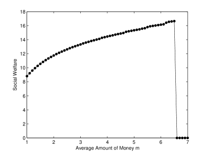
Figure 1: Social welfare for various average amounts of money, demonstrating a monetary crash.

Corollary 1 tells us that this crash is a very sharp phenomenon; with some amount of money the system performs well, but with just slightly more the system stops working. This is a result of the way increasing the amount of money affects agent’s best reply functions. Figure 2, reproduced from our companion paper Kash et al (2012), gives an example of a best reply function with one type of agent. It shows, for a particular fixed value of $m$, how the optimal strategy for an agent depends on the the strategies of the other agents. Thus, an equilibrium is a point on the line $y=x$: the optimal strategy is exactly the strategy the other agents are using. In this simple case, increasing $m$ causes every point to shift downward (since strategies are discrete, there may be some minimum increase for a particular point to shift). With a large enough increase in $m$, every point except (0,0) will be below the line and so there will be no nontrivial equilibrium. The sharpness is a result of there being a critical value $m^{*}$ at which the last point drops below the line.

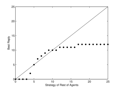
Figure 2: A hypothetical best-reply function with one type of agent.

In light of Corollary 1, the system designer should try to find $m^{*}$, the point where social welfare is maximized. In doing so, it is helpful to have an understanding of the types and strategies of agents in the systems, an issue we discuss in Section 6. In practice, the system designer may want to set the average amount of money $m$ to be somewhat less than $m^{*}$. Since there will be a crash if $m>m^{*}$, small changes in the characteristics of the population or mistakes by the designer in modeling them could lead to a crash if she chooses $m$ too close to $m^{*}$.

The phenomenon of a monetary crash is intimately tied to our assumption of fixed prices. We saw such a crash in practice in the babysitting co-op example. If the price is allowed to float freely, we expect that, as the money supply increases, there will be inflation; the price will increase so as to avoid a crash. However, floating prices can create other monetary problems, such as speculation, booms, and busts. Floating prices also impose transaction costs on agents. In systems where prices would normally be relatively stable, these transaction costs may well outweigh the benefits of floating prices, so a system designer may opt for fixed prices, despite the risk of a crash.

We believe there may also be a happy medium between a single, permanent fixed price and prices that change freely from round to round; indeed, our advice to system designers points naturally toward it. In particular, our advice about how to optimize the amount of money relies on experimentation and observation to determine what agents are doing and what their utilities are. This information then tells the designer how much money she should provide. Since adjusting the amount of money is equivalent to adjusting prices, the designer could incorporate this process into a price setting rule. Depending on the nature of the system, this could either be done manually over time (if the information is difficult to gather and analyze) or automatically (if the information gathering and analysis can itself be automated). From this perspective, a monetary crash, though real, is not something to be feared. Instead, it is just a strong signal that the current price, while probably not too far off from a very good price, requires adjustment. Naturally, this relies on a process that proceeds slow enough that agents myopically ignore the effects of future price changes in determining their current action.

Finally, a system designer could consider interventions other than adjusting the amount of money. One obvious opportunity is the process by which volunteers are selected. Our model assumes this process is random, but it need not be. For example, the system designer could attempt to bias the process in favor of agents with smaller amounts of money. Like increasing the average amount of money, this could increase efficiency since agents would spend less time with no money, but could potentially cause a crash, since agents have less of an incentive to save for the future. Our techniques rely on the choice of agents being independent of how much money they have, do not allow us to rigorously analyze this situation. Biasing the volunteer selection rule is an idea we return to in Section 5.3, as agents who create sybils increase their probability of being chosen.

5 Dealing with Nonstandard Agents

The model in Section 2 defines the utility of standard agents, who value service and dislike using their resources to provide it to others. This seems like a natural description of the way most people use distributed systems. However, in a real system, not every user will behave they way the designer intends. A practical system needs to be robust to nonstandard behaviors. In this section, we show how our model can be used to understand the effects of four interesting types of nonstandard behavior. First, an agent might provide service even when he will receive nothing in return, behaving as an altruist. Second, rather than viewing money as a means to satisfy future requests, an agent might place an inherent value on it and start hoarding it. Third, an agent might create additional identities, known as sybils, to try and manipulate the system. Finally, agents might collude with each other.

The results of this section give a system designer insight into how to design a scrip system that takes into account (and is robust to) a number of frequently-observed behaviors.

5.1 Altruists

P2P filesharing systems often have large numbers of free riders; they work because a small number of altruistic users provide most of the files. For example, Adar and Huberman 2000 found that, in the Gnutella network, nearly 50 percent of responses are from the top 1 percent of sharing hosts. A wide variety of systems have been proposed to discourage free riding. However, according to our model, unless this system mostly eliminates the altruistic users, adding such a system will have no effect on rational users.

To make this precise, take an altruist to be someone who always volunteers to fulfill requests, regardless of whether the other agent can pay. Agent $i$ might rationally behave altruistically if, rather than suffering a loss of utility when satisfying a request, $i$ derives positive utility from satisfying it. Such a utility function is a reasonable representation of the pleasure that some people get from the sense that they provide the music that everyone is playing. For such altruistic agents, the strategy of always volunteering is dominant. While having a nonstandard utility function might be one reason that a rational agent might use this strategy, there are certainly others. For example a naive user of filesharing software with a good connection might well follow this strategy. All that matters for the following discussion is that there are some agents that use this strategy, for whatever reason. For simplicity, we assume that all such agents have the same type $t_{a}$.

Suppose that a system has $a$ altruists. Intuitively, if $a$ is moderately large, they will manage to satisfy most of the requests in the system even if other agents do no work. Thus, there is little incentive for any other agent to volunteer, because he is already getting full advantage of participating in the system. Based on this intuition, it is a relatively straightforward calculation to determine a value of $a$ that depends only on the types, but not the number $n$, of agents in the system, such that the dominant strategy for all standard agents $i$ is to never volunteer to satisfy any requests.

Proposition 1

For all games $(T,\vec{f},h,m,1)$ with $f_{t_{a}}>0$, there exists a value $a$ such that, if $n>a/(f_{t_{a}}h)$ (i.e., there are at least $a$ altruists), then never volunteering is a dominant strategy for all standard agents.

Proof

Consider the strategy for a standard agent $i$ in the presence of $a$ altruists. Even with no money, agent $i$ will get a request satisfied with probability $1-(1-\beta_{t_{a}})^{a}$ just through the actions of the altruists. Consider a round when agent $i$ is chosen to make a request. If he has no money (because he never volunteered), his expected utility is $\gamma_{\tau(i)}(1-(1-\beta_{t_{a}})^{a})$. His maximum possible utility for the round is $\gamma_{\tau(i)}$. Thus, a strategy where he volunteers can increase his utility for a round by at most $\gamma_{\tau(i)}(1-\beta_{t_{a}})^{a}$. Thus, even if the agent gets every request satisfied, his expected utility can increase by at most

$$\begin{array}[]{ll}&(1-\delta_{\tau(i)})\sum_{r=0}^{\infty}\frac{\rho_{\tau(i)}}{hn}\gamma_{\tau(i)}(1-\beta_{t_{a}})^{a}(1-\frac{1-\delta_{\tau(i)}}{n})^{r}\\ =&(1-\delta_{\tau(i)})(\rho_{\tau(i)}/h)\gamma_{\tau(i)}(1-\beta_{t_{a}})^{a}/(1-\delta_{\tau(i)})\\ =&(\rho_{\tau(i)}/h)\gamma_{\tau(i)}(1-\beta_{t_{a}})^{a}.\end{array}$$

Clearly this expression goes to 0 as $a$ goes to infinity. If we take $a$ large enough that the expression is less than $\alpha_{t}$ for all types $t$, then the value of having every future request satisfied is less than the cost of volunteering now, so no agent will ever volunteer.  

Consider the following reasonable values for our parameters: $\beta_{t}=.01$ (so that each player can satisfy 1% of the requests), $\gamma_{t}=1$, $\alpha_{t}=.1$ (a low but non-negligible cost), $\delta_{t}=.9999$/day (which corresponds to a yearly discount factor of approximately $0.95$), and an average of 1 request per day per player. Then as long as $a>1145$ to ensure that not volunteering is a dominant strategy. While this is a large number, it is small relative to the size of a large P2P network. While the number of altruists needed to degrade the performance of the system increases somewhat with the number of agents, the point remains that a small fraction of altruists can discourage the rest of the system from providing service.

Proposition 1 shows that with enough altruists, the system eventually experiences a monetary crash, since all agents will use a threshold of zero. However, interesting behavior can still arise with smaller numbers of altruists. consider the situation where an $a$ fraction of requests are immediately satisfied at no cost without the requester needing to ask for volunteers. Intuitively, these are the requests satisfied by the altruists, although the following result also applies to any setting where agents occasionally have a (free) outside option. The following theorem shows that social welfare is increasing in $a$.

Let $G=(\{t\},1,h,m,n)$ be a game with a single type for which the standard conditions hold. Consider the family $G_{a}$ of games (parameterized by $a$) that result from $G$ if a fraction $a$ of requests can be satisfied at no cost. That is, the game $G_{a}$ is the same as $G$, except that if an agent $i$ makes a request, with probability $a$, it is satisfied at no cost, and with probability $1-a$, an agent is chosen among the volunteers to satisfy the request, just as in $G$, and the $i$ is charged 1 dollar to have the request satisfied.

Theorem 5.1

For the interval of values of $a$ where there is no monetary crash in $G_{a}$, social welfare increases as $a$ increases (assuming that the greatest equilibrium is played by all agents in $G_{a}$).

Proof

An agent’s utility in a round where he makes a request and it is satisfied at no cost is $\gamma_{t}$. Since such rounds occur with probability $a$, by assumption, our normalization guarantees that the sum of standard agents’ expected utilities in rounds where a request is satisfied at no cost is $a\gamma_{t}$. The same analysis as in Section 4 shows that the sum of agents’ expected utilities in each of the remaining rounds is $(1-a)(1-\zeta(a))(\gamma_{t}-\alpha_{t})$, where, as before, $\zeta(a)=d^{*}(t,0,a)$, the equilibrium value of $d^{*}(t,0)$ in the game $G_{a}$. Thus, expected utility as a function of $a$ is

$$a\gamma_{t}+(1-a)(1-\zeta(a))(\gamma_{t}-\alpha_{t}).$$ (6)

To see that this expression increases as $a$ increases, we would like to take the derivative relative to $a$ and show it is positive. Unfortunately, $\zeta(a)$ may not even be continuous. Because strategies are integers, there will be regions where $\zeta(a)$ is constant, and then a jump when a critical value of $a$ is reached that causes the equilibrium to change. At a point $a$ in a region where $\zeta(a)$ is constant, $\zeta^{\prime}(a)=0$, so the derivative of Equation (6) is $\gamma_{t}-(1-\zeta(a))(\gamma_{t}-\alpha_{t})>0$. Hence, social welfare is increasing at such points.

Now consider a point $a$ where $\zeta(a)$ is discontinuous. Such a discontinutity occurs when the greatest equilibrium, the greatest value $\vec{k}$ for which $\mathit{BR}_{G_{a}}(\vec{k})=\vec{k}$, changes. We show that, for a fixed $\vec{k}$, $\mathit{BR}_{G_{a}}(\vec{k})$ is non-increasing in $a$. Since increasing $a$ can only cause the $\mathit{BR}_{G_{a}}(\vec{k})$ to decrease, the discontinuity must be caused by a change from an equilibrium $\vec{k}$ to a new equilibrium $\vec{k}^{\prime}<\vec{k}$. Fix a vector $\vec{k}$ of thresholds, and let $p_{u}^{\vec{k},m,a}$ be the probability that $i$ will earn a dollar in a given round if he is willing to volunteer, given that a fraction $a$ of requests is satisfied at no cost (so that $p_{u}^{\vec{k},m,0}$ is what we earlier called $p_{u}^{\vec{k},m}$); we similarly define $p_{d}^{\vec{k},m,a}$, his probability of being chosen to make a request. It is easy to see that $p_{u}^{\vec{k},m,a}=(1-a)p_{u}^{\vec{k},m,0}$ and $p_{d}^{\vec{k},m,a}=(1-a)p_{d}^{\vec{k},m,0}$. The random variable $J(\kappa,p_{u},p_{d})$ in Equation (4) describes the first time at which an agent starting with $\kappa$ dollars and using the threshold $\kappa$ while earning a dollar with probability $p_{u}$ and spending a dollar with probability $p_{d}$ reaches zero dollars. As $a$ increases, $p_{u}^{\vec{k},m,a}$ and $p_{d}^{\vec{k},m,a}$ both decrease, but the ratio $p_{u}^{\vec{k},m,a}/p_{d}^{\vec{k},m,a}$ remains constant. Intuitively, this means that the agent “slows down” his random walk on amounts of money by a factor of $1/(1-a)$. This slowdown occurs because, each time the agent would have an opportunity to volunteer or would have spent a dollar, with probability $a$ the opportunity is taken by an altruist instead, so the expected time to take a step increases by a factor of $1/(1-a)$. Thus, the value of the expectation in Equation (4), and hence the right-hand side of Equation (4), decreasing as a function of $a$. By Lemma 3, $(\mathit{BR}_{G_{a}}(\vec{k}))_{t}$ is the maximum value of $\kappa$ such that Equation (4) is satisfied. Decreasing the right-hand side can only decrease the maximum value of $\kappa$, so $\mathit{BR}_{G_{a}}(\vec{k})$ is non-increasing as a function of $a$.

By Lemma 4, $\lambda_{m,\vec{k}}$ is non-increasing in $\vec{k}$ (unless the system crashes, after which it remains crashed even when a is increased further, as in Corollary 1, where the points at which social welfare is increasing form an interval). Since, as we have just shown, if there is a discontinuity at $\zeta(a)$ when $a$ increases, the greatest equilibrium changes at $a$ from $\vec{k}$ to $\vec{k}^{\prime}<\vec{k}$, we must have $\lambda_{m,\vec{k}^{\prime}}\geq\lambda_{m,\vec{k}}$. In Equation (2) for $i=0$, the value of the numerator is independent of $\lambda$, but the denominator with $\lambda_{m,\vec{k}^{\prime}}$ is greater than or equal to the denominator with $\lambda_{m,\vec{k}}$. Thus $d^{*}(t,0,a)=\zeta(a)$ is non-increasing at $a$. By Equation (6), this means that expected utility is increasing at $a$. Thus, in either case, social welfare is increasing in $a$.  

Theorem 5.1 and Proposition 1 combine to tell us that a little altruism is good for the system, but too much causes a crash. Figure 3 demonstrates this phenomenon. As we saw in Section 4, such crashes are caused when $m$, the average amount of money, is too large. By decreasing $m$ appropriately, even relatively large values of $a$ can be exploited, as Figure 4 shows. The “social welfare without adjustment” plot is the same data from Figure 3, with the corresponding plot of the amount of money horizontal since $m$ was held fixed. By decreasing the average amount of money appropriately as the number of altruists increases, a system designer can increase social welfare while avoiding a crash of the economy (the system will still function due to the presence of altruists). Note that, in discussing social welfare, our formulation excludes the welfare of the altruists, since our focus here is on the effects of altruism on standard agents.

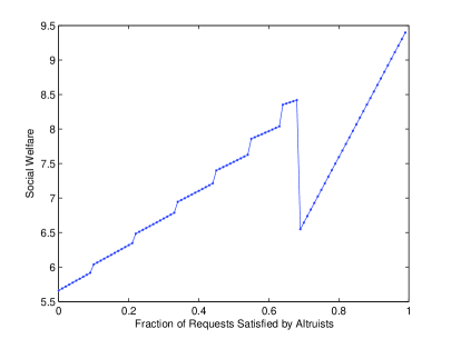
Figure 3: Altruists can cause a crash.

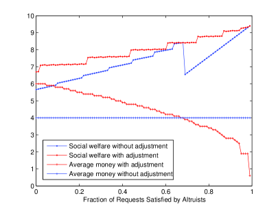
Figure 4: $m$ can be adjusted as $a$ increases.

5.2 Hoarders

Whenever a system allows agents to accumulate something, be it work done, as in SETI@home, friends on online social networking sites, or “gold” in an online game, a certain group of users seems to make it their goal to accumulate as much of it as possible. In pursuit of this, they will engage in behavior that seems irrational. For simplicity here, we model hoarders as playing the strategy $s_{\infty}$. This means that they will volunteer under all circumstances. Our analysis would not change significantly if we also required that they never made a request for work. Our first result shows that, for a fixed money supply, having more hoarders makes standard agents worse off.

Consider a game $G=(T,\vec{f},h,m,n)$ such that the standard conditions hold. Consider the family $G_{f_{h}}$ of games (parameterized by $f_{h}$) that result from $G$ if a fraction $f_{h}$ of agents are hoarders. That is, $G_{f_{h}}=(T\times\{0,1\},\vec{f}^{\prime},h^{\prime},m,n)$ where an agent of type $(t,0)$ is a standard agent of type $t$, but an agent of type $(t,1)$ is a hoarder and always uses the strategy $s_{\infty}$ (his probabilities are still determined by $\beta_{t}$, $\rho_{t}$, and $\chi_{t}$). Define $\vec{f}^{\prime}$ by taking $f_{(t,0)}^{\prime}=(1-f_{h})f_{t}$ and $f_{(t,1)}^{\prime}=f_{h}f_{t}$ for all types $t$. Let $h^{\prime}$ be the smallest multiple of $h$ such that $f_{(t,i)}h^{\prime}$ is an integer for all $t$ and $i$. (We need to adjust $h$ because otherwise the number of agents in the base game may not be well defined.) Finally, to account for the changed $h$, let $\delta_{(t,i)}=1-(1-\delta_{t})h/h^{\prime}$.

Theorem 5.2

In the family $G_{f_{h}}$ of games, social welfare is non-increasing in $f_{h}$ (if the greatest equilibrium is played by all agents in $G_{f_{h}}$).

Proof

Let $\vec{k}(f_{h})$ denote the greatest equilibrium in $G_{f_{h}}$. An increase in $f_{h}$ is equivalent to taking some number of standard agents and increasing their strategy to $s_{\infty}$. It follows from Lemma 4 that $\mathit{BR}_{G_{f_{h}}}$ is non-decreasing in $f_{h}$, and so $\vec{k}(f_{h})$ is non-decreasing in $f_{h}$. Again by Lemma 4, $\lambda_{m,\vec{k}(f_{h})}$ is non-increasing in $f_{h}$. Let $\zeta{f_{h}}=1/(1-f_{h})\sum_{t}d^{*}((t,0),0,f_{h})$ be the fraction of non-hoarders with zero dollars, where $d^{*}((t,0),0,f_{h})$ is the value of $d^{*}((t,0),0)$ at the greatest equilibrium of $G_{f_{h}}$. By Equation (2), $\zeta(f_{h})$ is non-decreasing in $f_{h}$. Thus, social welfare is non-increasing in $f_{h}$.  

Hoarders do have a beneficial aspect. As we have observed, a monetary crash occurs when a dollar becomes valueless, because there are no agents willing to take it. However, with hoarders in the system, there is always someone who will volunteer, so there cannot be a crash. Thus, for any $m$, the greatest equilibrium will be nontrivial and, by Theorem 4.1, social welfare keeps increasing as $m$ increases. So, in contrast to altruism, where the appropriate response was to decrease $m$, the appropriate response to hoarders is to increase $m$. In fact, our results indicate that the optimal response to hoarders is to make $m$ infinite. This is due to our unrealistic assumption that hoarders would use the strategy $s_{\infty}$ regardless of the value of $m$. There is likely an upper limit on the value of $m$ in practice, since it is unlikely that hoarders would be willing to hoard scrip if it is so easily available.

5.3 Sybils

Unless identities in a system are tied to a real world identity (for example by a credit card), it is effectively impossible to prevent a single agent from having multiple identities Douceur (2002). Nevertheless, there are a number of techniques that can make it relatively costly for an agent to do so. For example, Credence uses cryptographic puzzles to impose a cost each time a new identity wishes to join the system Walsh and Sirer (2006). Given that a designer can impose moderate costs to sybilling, how much more need she worry about the problem? In this section, we show that the gains from creating sybils when others do not diminish rapidly, so modest costs may well be sufficient to deter sybilling by typical users. However, sybilling is a self-reinforcing phenomenon. As the number of agents with sybils gets larger, the cost to being a non-sybilling agent increases, so the incentive to create sybils becomes stronger. Therefore, measures to discourage or prevent sybilling should be taken early before this reinforcing trend can start. Finally, we examine the behavior of systems where only a small fraction of agents have sybils. We show that under these circumstances a wide variety of outcomes are possible (even when all agents are of a single type), ranging from a crash (where no service is provided) to an increase in social welfare. This analysis provides insight into the tradeoffs between efficiency and stability that occur when controlling the money supply of the system’s economy.

When an agent of type $t$ creates sybils, the only parameter of his type that may change as a result is $\chi_{t}$, if we redefine the likelihood of an agent being chosen to be the likelihood of the agent or any of his sybils being chosen. The other parameters, such as $\rho$, remain unchanged because there is no particular reason that having multiple identities should cause the agent to, for example, desire service more often. For simplicity, we assume that each sybil is as likely to be chosen as the original agent, so creating $s$ sybils increases $\chi_{t}$ by $s\chi_{t}$. (Sybils may have other impacts on the system, such as increased search costs, but we expect these to be minor.)

Increasing $\chi_{t}$ benefits an agent by increasing his value of $\omega_{t}$ and thus $p_{u}$, his probability of earning a dollar (see Equation (8) in Appendix A). When $p_{u}<p_{d}$, the agent has more opportunities to spend money than to earn money, so he will regularly have requests go unsatisfied due to a lack of money. In this case, the fraction of requests he has satisfied is roughly $p_{u}/p_{d}$, so increasing $p_{u}$ by creating sybils results in a roughly linear increase in utility. As Theorem 5.3 shows, when $p_{u}$ is close to $p_{d}$, the increase in satisfied requests is no longer linear, so the benefit of increasing $p_{u}$ begins to diminish. Finally, when $p_{u}>p_{d}$, most of the agent’s requests are being satisfied, so the benefit from increasing $p_{u}$ is very small. Figure 5 illustrates an agent’s utility as $p_{u}$ varies for $p_{d}=.0001$. We formalize the relationship between $p_{u}$, $p_{d}$, and the agent’s utility in the following theorem, whose proof is deferred to Appendix B.

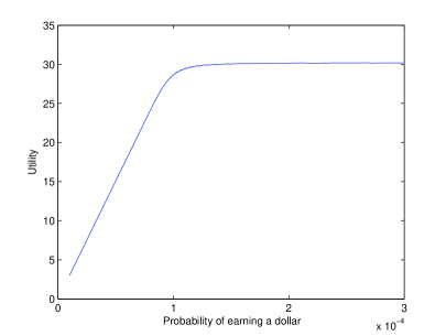
Figure 5: The effect of $p_{u}$ on utility

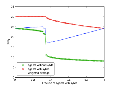
Figure 6: The effect of sybils on utility

Theorem 5.3

Fix a game $G$ and vector of thresholds $\vec{k}$. Let $R_{\vec{k},t}=p_{u}^{\vec{k},t}/p_{d}^{t}$. In the limit as the number of rounds goes to infinity, the fraction of the agent’s requests that have an agent willing and able to satisfy them that get satisfied is $(R_{\vec{k},t}-R_{\vec{k},t}^{k_{t}+1})/(1-R_{\vec{k},t}^{k_{t}+1})$ if $R_{\vec{k},t}\neq 1$ and $k_{t}/(k_{t}+1)$ if $R_{\vec{k},t}=1$.

Theorem 5.3 gives insight into the equilibrium behavior with sybils. Clearly, if sybils have no cost, then creating as many as possible is a dominant strategy. However, in practice, we expect there is some modest overhead involved in creating and maintaining a sybil, and that a designer can take steps to increase this cost without unduly burdening agents. With such a cost, adding a sybil might be valuable if $p_{u}$ is much less than $p_{d}$, and a net loss otherwise. This makes sybils a self-reinforcing phenomenon. When a large number of agents create sybils, agents with no sybils have their $p_{u}$ significantly decreased. This makes them much worse off and makes sybils much more attractive to them. Figure 6 shows an example of this effect. This self-reinforcing quality means that it is important to take steps to discourage the use of sybils before they become a problem. Luckily, Theorem 5.3 also suggests that a modest cost to create sybils will often be enough to prevent agents from creating them because with a well chosen value of $m$, few agents should have low values of $p_{u}$.

We have interpreted Figures 5 and 6 as being about changes in $\chi$ due to sybils, but the results hold regardless of what caused differences in $\chi$. For example, agents may choose a volunteer based on characteristics such as connection speed or latency. If these characteristics are difficult to verify and do impact decisions, our results show that agents have a strong incentive to lie about them. This also suggests that the decision about what sort of information the system should enable agents to share involves tradeoffs. If advertising legitimately allows agents to find better service or more services they may be interested in, then advertising can increase social welfare. But if these characteristics impact decisions but have little impact on the actual service, then allowing agents to advertise them can lead to a situation like that in Figure 6, where some agents have a significantly worse experience.

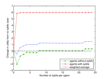
Figure 7: Sybils can improve utility

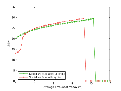
Figure 8: Sybils can cause a crash

We have seen that when a large fraction of agents have sybils, those agents without sybils tend to be starved of opportunities to work (i.e. they have a low value of $p_{u}$). However, as Figure 6 shows, when a small fraction of agents have sybils this effect (and its corresponding cost) is small. Surprisingly, if there are few agents with sybils, an increase in the number of sybils these agents have can actually result in a decrease of their effect on the other agents. Because agents with sybils are more likely to be chosen to satisfy any particular request, they are able to use lower thresholds and reach those thresholds faster than they would without sybils, so fewer are competing to satisfy any given request. Furthermore, since agents with sybils can almost always pay to make a request, they can provide more opportunities for other agents to satisfy requests and earn money. Social welfare is essentially proportional to the number of satisfied requests (and is exactly proportional to it if everyone shares the same values of $\alpha$ and $\gamma$), so a small number of agents with a large number of sybils can improve social welfare, as Figure 7 shows. Note that, although social welfare increases, some agents may be worse off. For example, for the choice of parameters in this example, social welfare increases when twenty percent of agents create at least two sybils, but agents without sybils are worse off unless the twenty percent of agents with sybils create at least eight sybils. As the number of agents with sybils increases, they start competing with each other for opportunities to earn money and so adopt higher thresholds, and this benefit disappears. This is what causes the discontinuity in Figure 6 when approximately a third of the agents have sybils.

This observation about the discontinuity also suggests another way to mitigate the negative effects of sybils: increase the amount of money in the system. This effect can be seen in Figure 8, where for $m=2$ social welfare is very low with sybils but by $m=4$ it is higher than it would be without sybils.

Unfortunately, increasing the average amount of money has its own problems. Recall from Section 4 that, if the average amount of money per agent is too high, the system will crash. It turns out than just a small number of agents creating sybils can have the same effect, as Figure 8 shows. With no sybils, the point at which social welfare stops increasing and the system crashes is between $m=10.25$ and $m=10.5$ (we only calculated social welfare for values of $m$ that are multiples of 0.25, so we do not know the exact point of the crash). If one-fifth of the agents each create a single sybil, the system crashes if $m=9.5$, a point where, without sybils, the social welfare was near optimal. Thus, if the system designer tries to induce optimal behavior without taking sybils into account, the system will crash. Moreover, because of the possibility of a crash, raising $m$ to tolerate more sybils is effective only if $m$ was already set conservatively.

This discussions shows that the presence of sybils can have a significant impact on the tradeoff between efficiency and stability. Setting the money supply high can increase social welfare, but at the price of making the system less stable. Moreover, as the following theorem shows, whatever efficiencies can be achieved with sybils can be achieved without them, at least if there is only one type of agent. In the theorem, we consider a system where all agents have the same type $t$. Suppose that some subset of the agents have created sybils, and all the agents in the subset have created the same number of sybils. We can model this by simply taking the agents in the subsets to have a new type $s$, which is identical to $t$ except that the value of $\chi$ increases. Thus, we state our results in terms of systems with two types of agents, $t$ and $s$.

Theorem 5.4

Suppose that $t$ and $s$ are two types that agree except for the value of $\chi$, and that $\chi_{t}<\chi_{s}$. If $\vec{k}=(k_{t},k_{s})$ is an $\varepsilon$-Nash equilibrium for $G=(\{t,s\},\vec{f},h,m,n)$ with social welfare $w$, then there exist $h^{\prime}$, $m^{\prime}$, and $n^{\prime}$ such that $\vec{k}^{\prime}=(k_{s})$ is an $\varepsilon$-Nash equilibrium for $G^{\prime}_{h^{\prime},m^{\prime},n^{\prime}}=(\{t\},\{1\},h^{\prime},m^{\prime},n^{\prime})$ with social welfare greater than $w$.

We defer proof of Theorem 5.4 to Appendix B.

The analogous result for systems with more than one type of agent is not true. Figure 6 shows a game with a single type of agent, some of whom have created two sybils. However, we can reinterpret it as a game with two types of agents, one of whom has a larger value of $\chi$. With this reinterpretation, Figure 6 shows that social welfare is higher when all the agents are of the type $t_{h}$ with the higher value of $\chi$ than when only 40% are. Moreover, if only 40% of the agents have type $t_{h}$, social welfare would increase if the remaining agents created two sybils each (resulting in all agents having the higher value of $\chi$). Note that this situation, where there are two types of agents, of which one has a higher value of $\chi$, is exactly the situation considered by Theorem 5.4. Thus, the theorem shows that for any equilibrium with two such types of agents, there is a better equilibrium where one of those types creates sybils so as to effectively create only one type of agent.

While situations like this show that it is theoretically possible for sybils to increase social welfare beyond what is possible to achieve by simply adjusting the average amount of money, this outcome seems unlikely in practice. It relies on agents creating just the right number of sybils. For situations where such a precise use of sybils would lead to a significant increase in social welfare, a designer could instead improve social welfare by biasing the algorithm agents use for selecting which volunteer will satisfy the request.

Thus far, we have assumed that when agents create sybils the amount of money in the system does not change. However, the presence of sybils increases the number of apparent agents in the system. Since social welfare depends on the average amount of money per agent, if the system designer mistakes these sybils for an influx of new users and increases the money supply accordingly, she will actually end up increasing the average amount of money in the system, and may cause a crash. This emphasizes the need for continual monitoring of the system rather that just using simple heuristics to set the average amount of money, an issue we discuss more in Section 6.

5.4 Collusion

Agents that collude gain two major benefits. The primary benefit is that they can share money, which makes them less likely to run out of money (and hence unable to make a request), and allows them to pursue a joint strategy for determining when to work. A secondary benefit, but important in particular for larger collusive groups, is that they can satisfy each other’s requests. The effects of collusion on the rest of the system depend crucially on whether agents are able to volunteer to satisfy requests when they personally cannot satisfy the request but one of their colluding partners can. In a system where a request is for computation, it seems relatively straightforward for an agent to pass the computation to a partner to perform and then pass the answer back to the requester. On the other hand, if a request is a piece of a file it seems less plausible that an agent would accept a download from an unexpected source, and it seems wasteful to have the chosen volunteer download it for the sole purpose of immediately uploading it. If it is possible for colluders to pass off requests in this fashion, they are able to effectively act as sybils for each other, with all the consequences discussed in Section 5.3. However, if agents can volunteer only for requests they can personally satisfy, the effects of collusion are almost entirely positive.

Since we have already discussed the consequences of sybils, we will assume that agents are able to volunteer only to satisfy requests that they personally can satisfy. Furthermore, we make the simplifying assumption that agents that collude are of the same type, because if agents of different types collude their strategic decisions become more complicated. For example, once the colluding group has accumulated a certain amount of money, it may wish to have only members with small values of $\alpha$ volunteer to satisfy requests; or when it is low on money, it may wish to deny use of money to members with low values of $\gamma$. This results in strategies that involve sets of thresholds rather than a single threshold. While there seems to be nothing fundamentally different about the situation, it makes calculations significantly more difficult.

With these assumptions, we now examine how colluding agents will behave. Because colluding agents share money and types, it is irrelevant which members actually perform work and have money. All that matters is the total amount of money the group has. This means that when the group needs money, everyone in the group volunteers for a job; otherwise, no one does. Thus, the group essentially acts like a single agent, using a threshold that is somewhat less than the sum of the thresholds that the individual agents would have used, because it is less likely that $c$ agents will make $ck$ requests in rapid succession than a single agent making $k$. Furthermore, some requests will not require scrip at all because they can potentially be satisfied by other members of the colluding group. When deciding whether the group should satisfy a member’s request or ask for an outside volunteer to fulfill it, the group must decide whether it should pay a cost of $\alpha$ to avoid spending a dollar. Since not spending a dollar is effectively the same as earning a dollar, the decision is already optimized by the threshold strategy; the group should always attempt to satisfy a request internally unless it is in a temporary situation where the group is above its threshold.

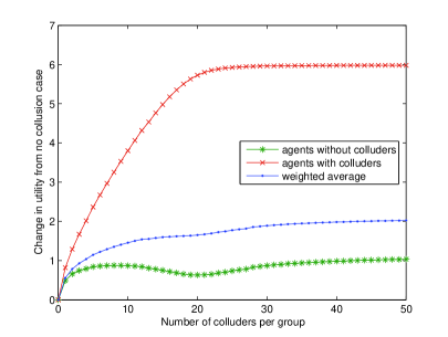
Figure 9: The effect of collusion on utility

Figure 9 shows an example of the effects of collusion on agents’ utilities as the size of collusive groups increases. As this figure suggests, the effects typically go through three phases. Initially, the fraction of requests colluders satisfy for each other is small. This means that each collusive group must work for others to pay for almost every request its members make. However, since they share money, the colluders do not have to work as often as individuals would. Thus, other agents have more opportunity to work, and every agent’s $p_{u}$ increases, making all agents better off.

As the number of colluders increases, the fraction of requests they satisfy internally grows significant. We can think of $p_{d}$ as decreasing in this case, and view these requests as being satisfied “outside” the scrip system because no scrip changes hands. This is good for colluders, but is bad for other agents whose $p_{u}$ is lower, since fewer requests are being made. Even in this range, non-colluding agents still tend to be better off than if there were no colluders, because the overall competition for opportunities to work is still lower. Finally, once the collusive group is large enough, it will have a low $p_{d}$ relative to $p_{u}$. This means the collusive group can use a very low threshold, which again begins improving utility for all agents. The analogous situation with sybils is transitory, and disappears when more agents create sybils. However, with collusion, this low threshold is an inherent consequence of colluders satisfying each other’s requests, and so persists and even increases as the amount of collusion in the system increases. Since collusion is difficult to maintain (the problem of incentivizing agents to contribute is the whole point of using scrip), we would expect the size of collusive groups seen in practice to be relatively small. Therefore, we expect that for most systems collusion will make no agent worse off, and some better off. Note that, as with sybils, the decreased in competition that results from collusion can also lead to a crash. However, if the system designer is monitoring the system, and encouraging and expecting collusion, she can reduce $m$ appropriately and prevent a crash.

These results also suggest that creating the ability to take out loans (with an appropriate interest rate) is likely to be beneficial. Loans gain the benefits of reduced competition without the accompanying cost of fewer requests being made in the system. However, implementing a loan mechanism requires addressing a number of other incentive problems. For example, whitewashing, where agents take on a new identity (in this case to escape debts) needs to be prevented Friedman and Resnick (2001).

6 Identifying User Strategies

Lemma 2 used relative entropy to derive an explicit formula for the distribution of money $d^{*}$ given a game $(T,\vec{f},h,n,m)$ and vector of strategies $\vec{k}$. In this section, we want to go in the opposite direction: given the distribution of money, we want to infer the strategies $\vec{k}$, the set of types present $T$, and the fraction of each type $\vec{f}$. For those interested in understanding the agents using a scrip system, knowing the fraction of agents using each strategy can provide a window into the preferences of those agents. For system designers, this knowledge is useful because, as we show in Section 4, how much money the system can handle without crashing depends on the fraction of agents of each type.

In equilibrium, the distribution of money has the form described in Lemma 2. Note that, in general, we do not expect to see exactly this distribution at any given time, but it follows from Theorem 3.1 that, after sufficient time, the distribution is unlikely to be very far from it. Does this distribution help us identify the strategies and types of agents?

As a first step to answering this question, given a distribution of money $d$ (where $d(i)$ is the fraction of agents with $i$ dollars) such that $d(i)$ is a rational number for all $i$ (this constraint is necessary if $d(i)$ is to represent the fraction of agents with $i$ dollars in a real system), suppose that the maximum amount of money to which $d$ gives positive probability is $K$. A vector $\vec{f}$ of length $K+1$ whose components are all rational numbers, where $f_{i}$ is intuitively the fraction of agents playing the threshold strategy $s_{i}$, is an explanation of $d$ if there exists a $\lambda$ such that

$$d(j)=\sum_{i}d_{\lambda}(i,j),$$

where

$$d_{\lambda}(i,j)=f_{i}\lambda^{j}/(\sum_{l=0}^{i}\lambda^{l})$$ (7)

if $j\leq i$ and 0 otherwise. Note that Equation (7) is very similar to Equation (2) from Lemma 2. In the following lemma, we show why we call $\vec{f}$ an explanation: given a distribution $d$ and an explanation $\vec{f}$ we can find a game $G$ where $\vec{f}$ is the fraction of agents of each type and $d$ is the equilibrium distribution of money (by which we mean that the value of $d^{*}$ in Lemma 2 is such that $d(i)=\sum_{t}d^{*}(t,i)$). Note that this definition implicitly assumes that $w_{t}=1$ for all $t$, a point to which we return later.

Lemma 5

If $\vec{f}$ is an explanation for $d$, then there exists a game $G=(T,\vec{f},h,m,n)$ and vector $\vec{k}$ of thresholds such that $\vec{k}$ is an $\varepsilon$-Nash equilibrium for $G$ and the equilibrium distribution of money is $d$.

Proof

Let $T=\{0,\ldots,K\}$, $h$ be the minimum integer such that $hd(i)$ is an integer for all $i$, $m=\sum_{i}id(i)$, and $\vec{k}$ be such that $k_{i}=i$. For each type $i$, choose $\beta_{i}$, $\chi_{i}$, and $\rho_{i}$ arbitrarily, subject to the constraint that $\beta\chi/\rho=1$ (so that, by definition, $\omega_{i}=1$ for all types $i$). Finally, choose an arbitrary $n$.

By Lemma 3, for any $n$, an optimal threshold policy in the MDP $\mathcal{P}_{G,\vec{S}(\vec{k}),i}$ for an agent of type $i$ is $s_{\kappa}$, where $\kappa$ is the maximum value such that

$$\alpha_{t}\leq E[(1-(1-\delta_{t})/n)^{J(\kappa,p_{u},p_{d})}]\gamma_{t}.$$ (4)

Fix $\delta_{i}$ and $\gamma_{i}$, and let $g(\kappa)$ be the sequence of values of the right hand side of Equation (4) for natural numbers $\kappa$. Recall that the random variable $J(\kappa,p_{u},p_{d})$ represents the round at which an agent starting with $\kappa$ dollars runs out of money. Since $J(0,p_{u},p_{d})=0$ for all histories, $g(0)=\gamma_{t}$. The time at which an agent runs out of money is increasing in his initial amount of money. Thus, $J(\kappa,p_{u},p_{d})$ is a strictly increasing function of $\kappa$, so $g(\kappa)$ is strictly decreasing. Choose $\alpha_{i}$ such that $g(i+1)<\alpha_{i}<g(i)$.

Thus, we have established parameters $(\alpha_{i},\beta_{i},\gamma_{i},\delta_{i},\chi_{i},\rho_{i})$ for each type $i$ so that $s_{i}$ an optimal policy for agents of type $i$ in the MDP $\mathcal{P}_{G,\vec{S}(\vec{k}),i}$. By Theorem 3.2, taking $n$ and the $\delta_{i}$ sufficiently large makes $\vec{k}$ a $\varepsilon$-Nash equilibrium for $G$. By Lemma 2, the equilibrium distribution of money is $d$.  

In general, there is not a unique explanation of a distribution $d$. Say that a distribution of money $d$ is fully-supported if there do not exist $i$ and $j$ such that $i<j$, $d(j)>0$, and $d(i)=0$. For any game $G$, if all agents play threshold strategies then the resulting distribution will be fully-supported because it has the form given in Lemma 2. As the following lemma shows, a fully-supported distribution can be explained in an infinite number of different ways.

Lemma 6

If $d$ is a fully-supported distribution of money with finite support, then there exist an infinite number of explanations of $d$.

We defer the proof of Lemma 6 to Appendix C.

Lemma 6 shows that $d$ has an infinite number of explanations. Lemma 5 shows that we can find an (approximate) equilibrium corresponding to each of them. The explanations $\vec{f}$ we construct in the proof of Lemma 6 seem unnatural; typically $f_{i}>0$ for all $i$. We are interested in a more parsimonious explanation, one that has a small support (i.e., the number of thresholds $i$ for which $f_{i}>0$ is small), for reasons the following lemma makes clear.

Lemma 7

Let $\vec{f}$ be an explanation for $d$. If $s$ is the size of the support of $\vec{f}$, then any other explanation will have a support of size at least $K-s$.

Proof

Suppose that $\vec{f}$ is an explanation for $d$. By Lemma 5, there is a game $G=(T,\vec{f},h,m,n)$ and vector $\vec{k}$ of thresholds such that $\vec{k}$ is an $\epsilon$-Nash equilibrium for $G$ and the equilibrium distribution of money is $d$. Moreover, the proof of Lemma 5 shows that we can take $T=\{0,\ldots,K\}$, $k_{i}=i$, and $\omega_{i}=1$ for each type $i\in T$. By Equation (2) in Lemma 2, $d^{*}(t,i)=f_{t}\lambda^{i}q(t,i)/\sum_{j=0}^{k_{t}}\lambda^{j}q(t,j)$, where $\lambda$ is the (unique) value that satisfies Equation (3). We first show that if $f_{i-1}=0$, then $d(i)/d(i-1)=\lambda$. Since, for all $i$, $\omega_{i}=1$, it is immediate from the definition of $q$ for Lemma 2 that $q(i,j)=q(i,j^{\prime})$ for all $j$ and $j^{\prime}$. Thus, the $q$ terms cancel, so $d^{*}(i,j)=f_{i}\lambda^{j}/\sum_{l=0}^{k_{i}}\lambda^{l}$. Let $b_{i}=f_{i}/\sum_{l=0}^{k_{i}}\lambda^{l}$; then $d^{*}(i,j)=\lambda^{j}b_{i}$. Only agents with a threshold of at least $j$ can have $j$ dollars, so

$$d(j)=\sum_{j}d^{*}(i,j)=\sum_{\{t_{l}:l\geq j\}}d^{*}(l,j)=\sum_{\{t_{l}:l\geq j\}}b_{l}\lambda^{j}=B_{j}\lambda^{j},$$

where $B_{j}=\sum_{\{t_{l}:l\geq i\}}b_{l}$. If $f_{{i-1}}=0$, then $B_{i}=B_{i-1}$, so $d(i)/d(i-1)=\lambda$.

Since $s$ strategies get positive probability according to $\vec{f}$, at least $k-s$ of the ratios $d(i)/d(i-1)$ with $1\leq i\leq K$ must have value $\lambda$. Any other explanation $\vec{f}^{\prime}$ will have different coefficients $f_{i}$ in Equation (7), so the value $\lambda^{\prime}$ satisfying it will also differ (since the requirement that $d(K)=d_{\lambda}(K,K)$ uniquely defines a value of $\lambda$). This means that the $K-s$ ratios with value $\lambda$ must correspond to strategies $i$ such that $f_{i}>0$. Thus, the support of any other explanation must be at least $K-s$.  

If $s\ll K$, Lemma 7 gives us a strong reason for preferring the minimal explanation (i.e., the one with the smallest support); any other explanation will involve significantly more types of agents being present. For $s=3$ and $K=50$, the smallest explanation has a support of three thresholds, and thus requires three types; the next smallest explanation requires at least 47 types. Thus, if the number of types of agents is relatively small, the minimal explanation will be the correct one.

The proof of Lemma 7 also gives us an algorithm for finding this minimal explanation. Since $d(i)=B_{i}\lambda^{i}$, taking logs of both sides, $\log d(i)=\log B_{i}+i\log\lambda$. Because $B_{i}$ is constant in ranges of $i$ where $f_{t_{i}}=0$, a plot of $\log d(i)$ will be a line with slope $\lambda$ in these ranges. Thus, the minimal explanation can be found by finding the minimum number of lines of constant slope that fit the data. For a simple example of how such a distribution might look, Figure 10 shows an equilibrium distribution of money for the game

$$(\{(.05,1,1,.95,1),(.15,1,1,.95,1)\},(.3,.7),10,4,100)$$

so the only difference between the types is that it costs the second type three times as much to satisfy a request) and the equilibrium strategy profile $(20,13)$. Figure 11 has the same distribution plotted on a log scale. Note the two lines with the same slope ($\lambda$) and the break at 13.

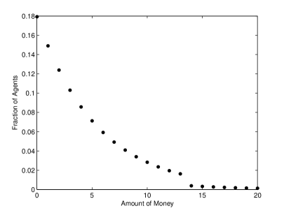
Figure 10: Distribution of money with two types of agents.

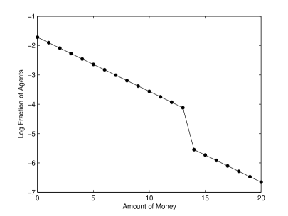
Figure 11: Log of the distribution of money with two types of agents.

Our notion of an explanation requires that $\vec{f}$ satisfy Equation (7), which, unlike Equation (2), does not contain a $q(t,i)$ term. Thus, it implicitly assumes that for all types $t$, $\omega_{t}=1$. Note that the game $G$ in the proof of Lemma 7 was constructed so at to ensure that $\omega_{t}=1$ for all types $t$. When $\omega_{t}$ is allowed to differ, we no longer have the simple form for $B_{i}$ used in Lemma 7. This is because the types do not share the same value of $\omega_{t}$. However, for a single type $t$ it is the case that $d^{*}(t,i)/d^{*}(t,i-1)=\lambda\omega_{t}$. $\omega_{\tau(j)}$ can be estimated by observing the results of requests, so by observing a sufficient number of agents the system designer should be able to estimate the values $d^{*}(t,i)$ and $\omega_{t}$ for some type $t$ and thus learn $\lambda$. If several, but not all, types $t$ have a common value of $\omega_{t}$, the procedure above can be used to determine $f_{t}$ and $k_{t}$ for each type and the resulting value of $\lambda$.

This procedure allows us to use a distribution of money to infer the minimal explanation of the number of types of agents: the fraction of the population composed of each type, and the strategy each type is playing. (Note that we cannot distinguish multiple types with a shared $\omega_{t}$ playing the same strategy.) We would like to use this information to learn about the preferences of agents: their values of $\alpha_{t}$, $\gamma_{t}$, and $\delta_{t}$. Lemma 3 shows how we can do this. Once we find an explanation, the value of $\lambda$ determines $p_{u}^{t}$ and $p_{d}^{t}$ for each type $t$. Then Equation 4 puts constraints on the values of $\alpha_{t}$, $\beta_{t}$, and $\gamma_{t}$. Over time, if $T$, the set of types, remains constant, but $\vec{f}$, $n$, and $m$ all vary as agents join and leave the system, a later observation with a slightly would give another equilibrium with new constraints on the types of the agents. A number of such observations potentially reveal enough information to allow strong inferences about agent types.

Thus far we have implicitly assumed that there are only a small number of types of agents in a system. Given that a type is defined by six real numbers, it is perhaps more reasonable to assume that each agent has a different type, but there is a small number of “clusters” of agents with similar types. For example, we might believe that generally agents either place a high value or a low value on receiving service. While the exact value may vary, the types of two low-value agents or two high-value agents will be quite similar. We have also assumed in our analysis that all agents play their optimal threshold strategy. However, computing this optimum may be too difficult for many agents. Even ignoring computational issues, agents may have insufficient information about their exact type or the exact types of other agents to compute the optimal threshold strategy. Both the assumption that there are a few clusters of agents with similar, but not identical, types and the assumption that agents do not necessarily play their optimal threshold strategy, but do play a strategy close to optimal, lead to a similar picture of a system, which is one that we expect to see in practice: we will get clusters of agents playing similar strategies (that is, strategies with thresholds clustered around one value), rather than all agents in a cluster playing exactly the same strategy. This change has relatively little impact on our results. Rather than seeing straight lines representing populations with a sharp gap between them, as in Figure 11, we expect slightly curved lines representing a cluster of similar populations, with somewhat smoother transitions.

7 Discussion

In this paper, we have examined some of the practical implications of the the theoretical results about scrip systems from our companion paper Kash et al (2012). For those interested in studying the agents of scrip systems, our characterization of equilibrium distribution of money forms the basis for techniques relevant to inferring characteristics of the agents of a scrip system from the distribution of money. For a system designer, our results on optimizing the money supply provide a simple maxim: keep adding money until the system is about to experience a monetary crash.

We have also seen that our model can be used to understand the effects of nonstandard agent behavior on a scrip system. It provides insight into the effects of altruists and hoarders on a scrip system and guidance to system designers for dealing with them (less and more money respectively). Sybils are generally bad, but can typically be discouraged by imposing a moderate cost and possibly biasing the process for selecting a volunteer. On the other hand, collusion tends to be a net benefit and should be encouraged. Indeed, the entire purpose of the system is to allow users to collude and provide each other with service despite incentives to free ride.

We remark that we are not the first to study the effects of altruists, sybils, and collusion on system behavior (although we believe we are the first to study it in the context of scrip systems). Work on the evolution of cooperation stresses the importance of altruists willing to undertake costly punishment Hauert et al (2007). Yokoo et al. 2004 studied the effects of sybils in auctions. Solution concepts such as strong Nash equilibrium Aumann (1959) and $k$-$t$ robust equilibrium Abraham et al (2006) explicitly address collusion in games; Hayrapetyan et al. 2006 study collusion in congestion games and find cases where, as with scrip systems, collusion is actually beneficial.

Although we believe that our analysis should already provide a great deal of insight to a system designer hoping to use a scrip system, many interesting open questions remain for future work. To name a few:

• Our model makes a number of strong predictions about the agent strategies, distribution of money, and effects of variations in the money supply. It also provides techniques to help analyze characteristics of agents of a scrip system. It would be interesting to test these predictions on a real functioning scrip system to either validate the model or gain insight from where its predictions are incorrect.

• In many systems there are overlapping communities of various sizes that are significantly more likely to be able to satisfy each other’s requests. For example, in a P2P filesharing system, people are more likely to be able to satisfy the requests of others who share the same interests. It would be interesting to investigate the effect of such communities on the equilibrium of our system.

• It seems unlikely that altruism and hoarding are the only two types of “irrational” behavior we will find in real systems. Are there other major types that our model can provide insight into? Furthermore, it seems natural that the behavior of a very small group of agents should not be able to change the overall behavior of the system. Can we prove results about equilibria and utility when a small group follows an arbitrary strategy? This is particularly relevant when modeling attackers. See Abraham et al (2006) for general results in this setting.

8 Acknowledgments

We would like to thank Randy Farmer, Peter Harremoes, Shane Henderson, Jon Kleinberg, David Parkes, Dan Reeves, Emin Gün Sirer, Michael Wellman, and anonymous referees for helpful suggestions, discussions, and criticisms. Eric Friedman, Ian Kash, and Joseph Halpern are supported in part by NSF under grant ITR-0325453. Joseph Halpern is also supported in part by NSF under grants CTC-0208535, IIS-0812045, and IIS-0534064; by ONR under grant N00014-01-10-511; by the DoD Multidisciplinary University Research Initiative (MURI) program administered by the ONR under grants N00014-01-1-0795 and N00014-04-1-0725; and by AFOSR under grants F49620-02-1-0101, FA9550-08-1-0438, FA9550-05-1-0055, and FA9550-09-1-0266. Eric Friedman is also supported in part by NSF under grant CDI-0835706.

Appendix A Definition of the MDP

In this appendix, we repeat the formal definition of the MDP from our companion paper Kash et al (2012). Taking notation from Puterman 1994, we formally define the MDP $\mathcal{P}_{G,\vec{S}(\vec{k}),t}=\mbox{$(S,A,p(\cdot\mid s,a),r(s,a))$}$ that describes the game where all the agents other than $i$ are playing $\vec{S}(\vec{k})_{-i}$ and $i$ has type $t$.

• $S=\{0,\ldots,mhn\}$ is the set of possible states for the MDP (i.e., the possible amounts of money compatible with the distribution $d^{*}$).

• $A=\{0,1\}$ is the set of possible actions for the agent, where 0 denotes not volunteering and 1 denotes volunteering iff another agent who has at least one dollar makes a request.

• $p_{u}$ is the probability of earning a dollar, assuming the agent volunteers (given that all other agents have fixed their thresholds according to $\vec{k}$ and the distribution of money is exactly $d^{*}$. Each agent of type $t^{\prime}$ who wishes to volunteer can do so with probability $\beta_{t^{\prime}}$. Assuming exactly the expected number of agents are able to volunteer, $\upsilon_{t^{\prime}}=\beta_{t^{\prime}}(f_{t^{\prime}}-d^{*}(t^{\prime},k_{t^{\prime}}))n$ agents of type $t^{\prime}$ volunteer. Note that we are disregarding the effect of $i$ in computing the $\upsilon_{t^{\prime}}$, since this will have a negligible effect for large $n$. Using the $\upsilon_{t}$s, we can express $p_{u}$ as the product of two probabilities: that some agent other than $i$ who has a dollar is chosen to make a request and that $i$ is the agent chosen to satisfy it. Thus,

  $$p_{u}=\left(\sum_{t^{\prime}}\rho_{t^{\prime}}(f_{t^{\prime}}-d^{*}(t^{\prime},0))\right)\left(\frac{\chi_{t}\beta_{t}}{\sum_{t^{\prime}}\chi_{t^{\prime}}\upsilon_{t^{\prime}}}\right).$$ (8)

• $p_{d}$ is the probability of agent $i$ having a request satisfied, given that agent $i$ has a dollar. Given that all agents are playing a threshold strategy, if the total number $n$ of agents is sufficiently large, then it is almost certainly the case that some agent will always be willing and able to volunteer. Thus, we can take $p_{d}$ to be the probability that agent $i$ will be chosen to make a request; that is,

  $$p_{d}=\frac{\rho_{t}}{hn}$$ (9)

• $r(s,a)$ is the (immediate) expected reward for performing action $a$ in state $s$. Thus, $r(s,0)=\gamma_{t}p_{d}$ if $s>0$; $r(0,0)=0$; $r(s,1)=\gamma_{t}p_{d}-\alpha_{t}p_{u}$ if $s>0$; and $r(0,1)=-\alpha_{t}p_{u}$.

• $p(s^{\prime}\mid s,a)$ is the probability of being in state $s^{\prime}$ after performing action $a$ in state $s$; $p(s^{\prime}\mid s,a)$ is determined by $p_{u}$ and $p_{d}$; specifically, $p(s+1\mid s,1)=p_{u}$, $p(s-1\mid s,a)=p_{d}$ if $s>0$, and the remainder of the probability is on $p(s\mid s,a)$ (i.e., $p(s\mid s,a)=1-(p(s+1\mid s,1)+p(s-1\mid s,a)$).

• $u^{*}(s)$ is the expected utility of being in state $s$ if agent $i$ uses the optimal policy for the MDP $\mathcal{P}_{G,\vec{S}(\vec{k}),t}$

• $u(s,a)$ is the expected utility for performing action $a$ in state $s$, given that the optimal strategy is followed after this action;

  $$u(s,a)=r(s,a)+\delta\sum_{s^{\prime}=0}^{mhn}p(s^{\prime}\mid s,a)u^{*}(s^{\prime}).$$

Appendix B Proofs from Section 5

• Fix a game $G$ and vector of thresholds $\vec{k}$. Let $R_{\vec{k},t}=p_{u}^{\vec{k},t}/p_{d}^{t}$. In the limit as the number of rounds goes to infinity, the fraction of the agent’s requests that have an agent willing and able to satisfy them that get satisfied is $(R_{\vec{k},t}-R_{\vec{k},t}^{k_{t}+1})/(1-R_{\vec{k},t}^{k_{t}+1})$ if $R_{\vec{k},t}\neq 1$ and $k_{t}/(k_{t}+1)$ if $R_{\vec{k},t}=1$.

Proof

Consider the Markov chain $\mathcal{M}$ that results from fixing the agent’s policy to $s_{k_{t}}$ in $\mathcal{P}_{G,\vec{S}(\vec{k}),t}$. $\mathcal{M}$ satisfies the requirements to have a limit distribution (see Theorem A.1 of Kash et al (2012)). It can be easily verified that the distribution gives the agent probability $R^{i}(1-R)/(1-R^{k+1})$ of having $i$ dollars if $R\neq 1$ and probability $1/(k+1$) if $R=1$ satisfies the detailed balance condition and thus is the limit distribution. This gives the probabilities given in the theorem.  

• Suppose that $t$ and $s$ are two types that agree except for the value of $\chi$, and that $\chi_{t}<\chi_{s}$. If $\vec{k}=(k_{t},k_{s})$ is an $\varepsilon$-Nash equilibrium for $G=(\{t,s\},\vec{f},h,m,n)$ with social welfare $w$, then there exist $m^{\prime}$, and $n^{\prime}$ such that $\vec{k}^{\prime}=(k_{s})$ is an $\varepsilon$-Nash equilibrium for $G^{\prime}_{m^{\prime},n^{\prime}}=(\{t\},\{1\},h,m^{\prime},n^{\prime})$ with social welfare greater than $w$.

Proof

We prove the theorem by finding $m^{\prime}$, and $n^{\prime}$ such that agents in $G^{\prime}_{m^{\prime},n^{\prime}}$ that play some strategy $k$ get essentially the same utility that an agent with sybils would by playing that strategy in $G$. Since $k_{s}$ was the optimal strategy for agents with sybils in $G$, it must be optimal in $G_{m^{\prime},n^{\prime}}$ as well. Since agents with sybils have utility at least as great as those without, social welfare will be at least as large in $G^{\prime}_{m^{\prime},n^{\prime}}$ as in $G$. To do so, we find a value of $m^{\prime}$ so that, from his perspective, being in $G$ with sybils or $G^{\prime}$ without results in exactly the same MDP. The natural way to do so is to treat $m^{\prime}$ as a continuous value, which might result in a value such that $hm^{\prime}n$ (the total amount of money) is not an integer. To complete the proof, we show that an $n^{\prime}$ can be found that allows us to avoid this problem.

Since an agent can earn a dollar only if he is able to satisfy the current request, $0<p_{u}^{m,\vec{k},s}<\beta_{s}$. The constraint that $hm^{\prime}n^{\prime}$, the total amount of money, is a natural number means that $m^{\prime}$ must be a rational number. For the moment, we ignore that constraint and allow $m^{\prime}$ to take on any value in $[0,k_{t}^{\prime}]$. From Equation (8), $p_{u}^{m^{\prime},\vec{k}^{\prime},t}$ is continuous in $d^{*}_{q_{\vec{k}^{\prime}}}$, which, by Lemma 2, is continuous in $\lambda_{m^{\prime},\vec{k}^{\prime}}$ and thus $m^{\prime}$. We use this continuity to show that we can find a value of $m^{\prime}$ such that $p_{u}^{m,\vec{k},s}=p_{u}^{m^{\prime},\vec{k}^{\prime},t}$. By Equation (3), if $m^{\prime}=0$ then $d^{*}_{q_{\vec{k}^{\prime}},m}(t,0)=1$, and if $m^{\prime}=k_{t}^{\prime}$ then $d^{*}_{q_{\vec{k}^{\prime}},m}(t,k_{t}^{\prime})=1$. Combining these with Equation (8) gives $p_{u}^{0,\vec{k}^{\prime},t}=0$ and $p_{u}^{m^{\prime},\vec{k}^{\prime},t}=\beta_{t}.$ Thus, by the Intermediate Value Theorem, there exists an $m^{\prime}$ such that $p_{u}^{m,\vec{k},s}=p_{u}^{m^{\prime},\vec{k}^{\prime},t}$. For this choice of $m^{\prime}$, observe that by Lemma 3, $\mathcal{P}_{G,\vec{S}(\vec{k}),s}$ and $\mathcal{P}_{G_{m^{\prime}},\vec{S}(\vec{\kappa}^{\prime}),t}$ have the same optimal threshold policy.

If $m^{\prime}$ is rational, say $m^{\prime}=a/b$, take $n^{\prime}=bn$; then $hm^{\prime}n^{\prime}$ is an integer and, by the argument above, $\vec{k}^{\prime}$ is an equilibrium for $G_{m^{\prime},n^{\prime}}$. Since $p_{u}^{m^{\prime},\vec{k}^{\prime}}=p_{u}^{\vec{k},s}>p_{u}^{\vec{k},t}$, we must have $\zeta_{G_{m^{\prime},n^{\prime}}}<\zeta_{G}$. Thus, social welfare has increased. If $m^{\prime}$ is not rational, we instead use a rational value $m^{\prime\prime}$ sufficiently close to $m^{\prime}$ that $\vec{k}^{\prime}$ is still an equilibrium for $G_{m^{\prime},n^{\prime}}$ and $\zeta_{G_{m^{\prime\prime},n^{\prime\prime}}}<\zeta_{G}$.  

Appendix C Proof of Lemma 6

• If $d$ is a fully-supported distribution of money with finite support, there exist an infinite number of explanations of $d$.

Proof

Fix $\lambda$. The distribution $d$ and $\lambda$ determine an explanation $\vec{f}$ as follows. By Equation (7), we need $\vec{f}$ to satisfy $d(j)=\sum_{i=0}^{K}d_{\lambda}(i,j)$.

Recall that $K$ is the maximum value for which $d(K)>0$. Start by considering $f_{K}$. By the definition of $d_{\lambda}$, $d_{\lambda}(i,j)=0$ if $j>i$. Thus, the constraint becomes

$$d(K)=d_{\lambda}(K,K)=f_{K}\lambda^{K}/(\sum_{l=0}^{K}\lambda^{l}).$$

Take $f_{K}$ to be the unique value that satisfies this equation. Once we have defined $f_{K}$, again apply the constraint and take $f_{{K-1}}$ to be the unique value that satisfies

$$d(K-1) =d_{\lambda}(K,K-1)+d_{\lambda}({K-1},K-1)$$

$$=f_{K}\lambda^{K-1}/(\sum_{l=0}^{K}\lambda^{l})+f_{{K-1}}\lambda^{K-1}/(\sum_{l=0}^{K-1}\lambda^{l}).$$

Iterating this process uniquely defines $\vec{f}$ as the unique value that satisfies

$$d(j)=\sum_{i=j}^{K}d_{\lambda}(i,j)=\sum_{i=j}^{K}f_{i}\lambda^{j}/(\sum_{l=0}^{i}\lambda^{l}),$$

or

$$f_{i}=(\sum_{l=0}^{i}\lambda^{l})/\lambda^{i}\left(d(i)-\sum_{j=i+1}^{K}f_{j}\lambda^{i}/(\sum_{l=0}^{j}\lambda^{l})\right).$$

However, $\vec{f}$ may not be an explanation, since some $f_{j}$ may be negative. This happens exactly when

$$d(i)<\sum_{j=i+1}^{K}f_{j}\lambda^{i}/(\sum_{l=0}^{j}\lambda^{l}).$$ (10)

As $\lambda$ grows large, the right-hand side of (10) tends to 0. Since $d$ is fully-supported, we must have $d(i)>0$. Thus, we can ensure that (10) does not hold for any $i$ by taking $\lambda$ sufficiently large. Thus, for sufficiently large $\lambda$, $\vec{f}$ provides an explanation for $d$. Continuing to increase $\lambda$ will give an infinite number of different explanations.

References

- Abraham et al (2006) Abraham I, Dolev D, Gonen R, Halpern J (2006) Distributed computing meets game theory: Robust mechanisms for rational secret sharing and multiparty computation. In: 25th ACM Symp. on Principles of Distributed Computing (PODC), pp 53–62
- Adar and Huberman (2000) Adar E, Huberman BA (2000) Free riding on Gnutella. First Monday 5(10)
- Aperjis et al (2008) Aperjis C, Freedman MJ, Johari R (2008) Peer-assisted content distribution with prices. In: 2008 ACM Conference on Emerging Network Experiment and Technology (CoNEXT 2008), p 17
- Aumann (1959) Aumann RJ (1959) Acceptable points in general cooperative -person games. In: Tucker A, Luce R (eds) Contributions to the Theory of Games IV, Annals of Mathematical Studies 40, Princeton University Press, Princeton, N. J., pp 287–324
- Brunelle et al (2006) Brunelle J, Hurst P, Huth J, Kang L, Ng C, Parkes D, Seltzer M, Shank J, Youssef S (2006) Egg: An extensible and economics-inspired open grid computing platform. In: Third Workshop on Grid Economics and Business Models (GECON), pp 140–150
- Cover and Thomas (1991) Cover T, Thomas J (1991) Elements of Information Theory. John Wiley & Sons, Inc., New York
- Douceur (2002) Douceur JR (2002) The sybil attack. In: First International Workshop on Peer-to-Peer Systems (IPTPS), pp 251–260
- Friedman and Resnick (2001) Friedman EJ, Resnick P (2001) The social cost of cheap pseudonyms. Journal of Economics and Management Strategy 10(2):173–199
- Friedman et al (2006) Friedman EJ, Halpern JY, Kash IA (2006) Efficiency and Nash equilibria in a scrip system for P2P networks. In: Seventh ACM Conference on Electronic Commerce (EC 2006), pp 140–149
- Fudenberg and Tirole (1991) Fudenberg D, Tirole J (1991) Game Theory. MIT Press
- Gupta et al (2003) Gupta M, Judge P, Ammar MH (2003) A reputation system for peer-to-peer networks. In: Network and Operating System Support for Digital Audio and Video (NOSSDAV), pp 144–152
- Hauert et al (2007) Hauert C, Traulsen A, Brandt H, Nowak MA, Sigmund K (2007) Via freedom to coercion: The emergence of costly punishment. Science 316:1905–1907
- Hayrapetyan et al (2006) Hayrapetyan A, Tardos É, Wexler T (2006) The effect of collusion in congestion games. In: 38th Annual ACM Symposium on Theory of Computing, pp 89–98
- Hughes et al (2005) Hughes D, Coulson G, Walkerdine J (2005) Free riding on Gnutella revisited: The bell tolls? IEEE Distributed Systems Online 6(6)
- Ioannidis et al (2002) Ioannidis J, Ioannidis S, Keromytis AD, Prevelakis V (2002) Fileteller: Paying and getting paid for file storage. In: Financial Cryptography, pp 282–299
- Kash et al (2007) Kash IA, Friedman EJ, Halpern JY (2007) Optimizing scrip systems: Efficiency, crashes, hoarders and altruists. In: Eighth ACM Conference on Electronic Commerce (EC 2007), pp 305–315
- Kash et al (2009) Kash IA, Friedman EJ, Halpern JY (2009) Manipulating scrip systems: Sybils and collusion. In: First Conference on Auctions, Market Mechanisms and Their Applications (AMMA)
- Kash et al (2012) Kash IA, Friedman EJ, Halpern JY (2012) An equilibrium analysis of scrip systems, arxiv:1204.2942
- Krugman (1999) Krugman P (1999) The Accidental Theorist. Norton
- Mas-Colell et al (1995) Mas-Colell A, Whinston MD, Green JR (1995) Microeconomic Theory. Oxford University Press, Oxford, U.K.
- Miller and Drexler (1988) Miller MS, Drexler KE (1988) Markets and computation: Agoric open systems. In: Huberman B (ed) The Ecology of Computation, Elsevier, pp 133–175
- Peterson and Sirer (2009) Peterson RS, Sirer EG (2009) Antfarm: Efficient content distribution with managed swarms. In: Networked Systems Design and Implementation (NSDI)
- Puterman (1994) Puterman ML (1994) Markov Decision Processes. Wiley
- Reeves et al (2007) Reeves DM, Soule BM, Kasturi T (2007) Group decision making with Yootles, http://ai.eecs.umich.edu/people/dreeves/yootles/yootles.pdf
- Sirivianos et al (2007) Sirivianos M, Park JH, Chen R, Yang X (2007) Free-riding in BitTorrent networks with the large view exploit. In: Sixth International Workshop on Peer-to-Peer Systems (IPTPS)
- Stonebraker et al (1996) Stonebraker M, Aoki PM, Litwin W, Pfeffer A, Sah A, Sidell J, Stelin C, Yu A (1996) Mariposa: a wide-area distributed database system. The VLDB Journal 5(1):48–63
- Sweeney and Sweeney (1977) Sweeney J, Sweeney RJ (1977) Monetary theory and the great capitol hill babysitting co-op crisis: Comment. J of Money, Credit and Banking 9(1):86–89
- Vishnumurthy et al (2003) Vishnumurthy V, Chandrakumar S, Sirer EG (2003) KARMA: a secure economic framework for peer-to-peer resource sharing. In: First Workshop on Economics of Peer-to-Peer Systems (P2PECON)
- Walsh and Sirer (2006) Walsh K, Sirer EG (2006) Experience with an object reputation system for peer-to-peer filesharing. In: Third Symp. on Network Systems Design & Implementation (NSDI), pp 1–14
- Yokoo et al (2004) Yokoo M, Sakurai Y, Matsubara S (2004) The effect of false-name bids in combinatorial auctions: new fraud in internet auctions. Games and Economic Behavior 46(1):174–188
- Zhao et al (2005) Zhao S, Lo VM, GauthierDickey C (2005) Result verification and trust-based scheduling in peer-to-peer grids. In: Fifth IEEE International Conference on Peer-to-Peer Computing (P2P 2005), pp 31–38