First-principles modeling of temperature and concentration dependent solubility in the phase separating Fe_xCu_1-x alloy system

Abstract

We present a novel cluster-expansion (CE) approach for the first-principles modeling of temperature and concentration dependent alloy properties. While the standard CE method includes temperature effects only via the configurational entropy in Monte Carlo simulations, our strategy also covers the first-principles free energies of lattice vibrations. To this end, the effective cluster interactions of the CE have been rendered genuinely temperature dependent, so that they can include the vibrational free energies of the input structures. As a model system we use the phase-separating alloy Fe-Cu with our focus on the Fe-rich side. There, the solubility is derived from Monte Carlo simulations, whose precision had to be increased by averaging multiple CEs. We show that including the vibrational free energy is absolutely vital for the correct first-principles prediction of Cu solubility in the bcc Fe matrix: The solubility tremendously increases and is now in quantitative agreement with experimental findings.

First-principles modeling of phase stabilities of alloys is of scientific and technological importance. A major progress forward was made by the Cluster Expansion (CE) which is based on an Ising-like concept Sanchez et al. (1984); Ferreira et al. (1989); Müller (2003); Lerch et al. (2009). The power of CE consists in modeling concentration dependent properties of coherent alloy phases based on first-principles input information. For a system the energy $E_{\text{CE}}(\sigma)$ for a particular atomic configuration $\sigma$ with $N$ atoms is expanded in terms of hierarchical atomic arrangements such as points, pairs, triangles, and higher order objects. Those arrangements are called figures f, and the selected figure set is denoted by $\mathbb{F}$. The CE then reads

$$E_{\text{CE}}(\sigma)=N\sum_{\text{f}\in\mathbb{F}}D_{\text{f}}J_{\text{f}}{\Pi}_{\text{f}}(\sigma)~{},$$ (1)

in which the geometrically determined correlations ${\Pi}_{\text{f}}(\sigma)$ and the symmetry degeneracy $D_{\text{f}}$ are known for the given underlying parental crystal lattice. The unknown effective cluster interaction energies (ECIs) $J_{\text{f}}$, which are independent of $\sigma$, have to be extracted from some suitable input information, such as a set of density functional theory (DFT) structures, which are denoted by $\sigma\in\text{input}$. For those ordered structures the DFT calculations provide the ground state total energies $E_{0,\text{DFT}}(\sigma)$. Fitting the CE to the DFT results determines the unknown $J_{\text{f}}$. This is performed by a least-squares minimization of the residuals Lu et al. (1991), which in a simplified formulation Müller (2003); Lerch et al. (2009) reads

$$\sum_{\sigma\in\text{input}}|E_{\text{CE}}(\sigma)-E_{0,\text{DFT}}(\sigma)|^{2}\rightarrow\text{min}~{}.$$ (2)

The fit is validated by a (leave one out) cross validation score (CVS) van de Walle and Ceder (2002), which in turn drives a genetic algorithm (GA) in order to select the optimal figure set $\mathbb{F}$ for the given input Hart et al. (2005); Blum et al. (2005); Lerch et al. (2009). Additional input is provided until the CE is converged in a self-consistent way. If the CE in Eq. 1 converges reasonably fast and the fit in Eq. 2 is sufficiently accurate then DFT accuracy can be carried over to a configuration space much larger than the one defined by the DFT input. Finally, the combination of CE with Monte Carlo (MC) simulations allows a temperature dependent treatment of phase stabilities and related properties for a very large number of interacting atoms Kerscher et al. (2011).

So far, temperature only entered via the configurational entropy modeled by the MC simulation; other temperature dependent contributions were left out, e.g., the important vibrational free energies. In the following paragraphs, the present study will include the contributions from lattice vibrations and will demonstrate their strong influence on the phase stability.

Formally, it is obvious that the CE becomes temperature dependent when the ECIs become temperature dependent: $J_{\text{f}}\to J_{\text{f}}(T)$. This is the result when the ECIs in Eq. 2 are fitted to temperature dependent input energies. In the present case those are obtained by summing the temperature dependent vibrational free energy $F_{\text{vib},\text{DFT}}(\sigma,T)$ to the ground state total energy,

$$E_{\text{DFT}}(\sigma,T)=E_{0,\text{DFT}}(\sigma)+F_{\text{vib},\text{DFT}}(\sigma,T)\,,$$ (3)

in which $E_{0,\text{DFT}}(\sigma)$ is the outcome of a standard DFT calculation strictly valid only at $T=0$ K. The label “DFT” for $F_{\text{vib},\text{DFT}}(\sigma,T)$ indicates that it can be derived by the same DFT approach and accuracy as used for the total energy (see below for details). Other temperature dependent properties may be included by adding the corresponding temperature dependent terms, such as the magnetic ordering energy. However, such contributions are not included in the present study and—regarding the magnetic ordering—we assume perfect ferromagnetic ordering in terms of spin polarization. In order to include these temperature dependent effects, the CE is rewritten as

$$E_{\text{CE}}(\sigma)\,\to\,E_{\text{CE}}(\sigma,T)=N\sum_{\text{f}\in{\mathbb{F}(T)}}D_{\text{f}}J_{\text{f}}(T){\Pi}_{\text{f}}(\sigma)~{}.$$ (4)

Note, that the optimal set of figures has also become temperature dependent: $\mathbb{F}\to\mathbb{F}(T)$.

In the following, we will perform and discuss the temperature dependent form of the CE where the additionally included vibrational free energy is in general important for the phase stability of alloys and compounds Garbulsky and Ceder (1994); Craievich and Sanchez (1997); Stöhr et al. (2009). For this purpose the phase separating binary Fe_1-xCu_x alloy system at the Fe-rich side of the phase diagram is considered Franke and Neuschütz (1994). For such a system the application of CE needs particular care because no ground state line of ordered compounds exists, i.e. all formation energies are positive. Furthermore, besides the technological interest of hardening steel by alloying Fe with Cu, a previous study based on isolated single-atom and pairwise defects indicated that vibrational free energies are indeed influential on the solubility of Cu in an Fe matrix Reith and Podloucky (2009). Including vibrational contributions to CE has been previously discussed Walle and Ceder (2002) and applied in very few cases Ozoliņš et al. (1998); Yuge et al. (2008). The actual procedure, how to include the vibrational free energy is not unique. In the present work an approach is presented which—in combination with a fast and accurate procedure for deriving the phonon spectra—can be used in a convenient way for doing a CE and subsequent MC calculations.

The DFT calculations for the total energies were done by the Vienna ab initio simulation package (VASP) with the pseudopotential construction according to the projector augmented wave method Kresse and Joubert (1999); Kresse and Furthmüller (1996); Blöchl (1994). The exchange-correlation functional was treated within the generalized gradient approximation as parametrized by Perdew, Burke and Ernzerhof Perdew et al. (1996). All calculations were done spin polarized assuming ferromagnetic ordering of the Fe-atoms. Very good convergency of total energies and forces with respect to energy cutoffs and $\vec{k}$-point integration was ensured. Accurate forces were derived for calculating the phonon spectra and vibrational free energies by a direct force-constant method within the harmonic approximation as implemented in our program package fPHON, which is based on PHON Alfè (2009).

All the CE and DFT calculations were made for Fe-Cu alloys with a bcc parental lattice, since the main interest is in the Fe-rich part of the phase diagram below the ferrite to austenite transition. For pure Cu, also the fcc ground state total energy was calculated as a reference. For the CE the UNiversal CLuster Expansion (UNCLE) program package Lerch et al. (2009) was applied.

Initially, a standard CE for a bcc parental lattice was made utilizing only the DFT total energies for $T=0$ K. The results in Fig. 1 reveal that no stable binary phase for any composition exists, as it is expressed by the positive formation energies. As expected Franke and Neuschütz (1994); Reith and Podloucky (2009), the configurations with the lowest formation enthalpies (and the form of the ground-state line) correspond to phase separating atomic arrangements, which consist of slabs of pure Cu and Fe. In total, an input DFT set of 51 configurations was taken into account resulting in a CVS of $3.7$ meV/atom at $T=0$ K. The input set includes the energetically favorable structures as well as configurationally excited states in order to get reliable MC results, cf. Ref. (Seko et al., 2009). In Fig. 1, we let the CE predict the formation enthalpies of all 631 configurations $\sigma$ with unit cells up to 8 atoms large. The random mixing energy shown in Fig. 1 for $T=0$ K (no vibrational free energy included) agrees well with the result of Liu et al. Liu et al. (2005). With increasing temperature (i.e., including $F_{\text{vib},\text{DFT}}(\sigma,T)$ in the CE) the random energy is lowered and its maximum shifts to higher Cu concentrations, as shown in Fig. 1 for $T=1200$ K.

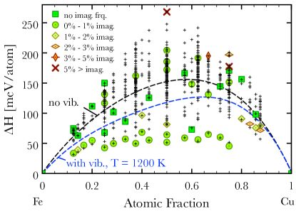
Figure 1: (color online) Enthalpy of formation derived from $E_{\text{CE/DFT}}(\sigma,T)$. DFT input values (various symbols) and CE predictions (black crosses) are compared. For the phonon calculations of each structure the percentage of imaginary frequencies is indicated. The random mixing energies are shown for $T=0$ K (standard CE, black dashed curve) and for $T=1200$ K (CE with vibrational free energy; blue dashed curve).

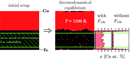
Figure 2: (color online) Cross section through the $50\times 50\times 50$ Monte Carlo simulation cell (Fe atoms: black, Cu: red). The initial setup of pure Cu and Fe blocks as shown on the left panel is brought into thermodynamical equilibrium for a fixed temperature (right part). The volume in the Fe block, in which the dissolved Cu atoms are counted, is indicated by two green borders, which are three layers away from the interface. This ensures that no Cu atom of the Cu slab is erroneously counted as dissolved. The right most panel demonstrates the concentration of dissolved Cu solubility per layer with and without $F_{\text{vib},{\text{DFT}}}(T)$. CE and MC calculations were made for the merged figure set using averaged ECIs (see text).

Including now $F_{\text{vib},\text{DFT}}(\sigma,T)$ for all 51 structures, Fig. 1 reveals that a considerable number of configurations have phonon spectra with imaginary frequencies, which indicates dynamical instability. Since all configurations are not thermodynamically stable anyway (they have positive formation enthalpies), this is not surprising. Anharmonic coupling of phonon modes might possibly stabilize some of the phonon modes Souvatzis et al. (2008), but such a task is forbiddingly expensive. Therefore, the usual assumption of neglecting non-vibrating modes in the vibrational free energy is made.

According to Eq. 4, different temperatures yield different $\mathbb{F}(T)$. However, one finds that the temperature dependence of the solubility is not as smooth a function of the temperature as expected. This is a direct effect of the GA Hart et al. (2005); Lerch et al. (2009) selecting the figure set $\mathbb{F}(T)$, and it can indeed be likened to that kind of arbitrariness which enters even at a single temperature: $n$ different runs of the GA yield $n$ different $\mathbb{F}_{i}(T)$. All of them are equally capable to map the input data onto the CE (Eq. 4) but yield slightly different results in MC simulations. For the usual CE applications, this does not pose a problem: the precision needed for MC simulations with respect to concentration is not as strict as needed here for the Cu solubility in Fe ($<1$ at.%), as we will see later on. In our case we need a strategy which allows us both to find the expected smooth behavior of the solubility and to increase the precision of the prediction.

We provide the following solution: an averaging procedure either of the results (i.e., the solubilities) or—more physically—of the CEs themselves. For each temperature, $n=10$ different CEs were constructed, with corresponding temperature dependent figure sets $\mathbb{F}_{i}(T)$ and energies $E_{\text{CE},i}(\sigma,T)$. For each CE $i$, a separate MC run was performed, where the simulation took place in a $50\times 50\times 50$ supercell, starting with the phase separated system by dividing the MC cell into blocks of pure Fe and Cu (see Fig. 2). This setup of fixed reservoirs of Cu and Fe atoms allows for an exchange of atoms between the two slabs using the Metropolis algorithm. Having reached thermal equilibrium at a given temperature, the solubility—i.e., the equilibrium concentration $x_{\text{s}}(\mathbb{F}_{i}(T))$ of dissolved Cu which depends slightly on the figure set $\mathbb{F}_{i}(T)$ used—is determined by counting the dissolved Cu atoms in bulk Fe as sketched in Fig. 2. For the different CEs, the solubility scatters around the averaged value $\bar{x}_{\text{s}}(\mathbb{F}_{i})=\sum_{i=1}^{n}x_{\text{s}}(\mathbb{F}_{i})/n$. Table 1 shows in the column $\bar{x}_{\text{s}}(\mathbb{F}_{i}(T))$ that the fluctuations become sizable at elevated temperatures because a high precision of the CE is needed to determine the Cu solubility at rather dilute concentrations. Therefore small fluctuations of the CE have a significant impact on the solubility.

Table 1: Results of 10 temperature dependent CE + MC runs and of one CE + MC with the merged figure set (see text). $N_{\text{f}}$ is the number of figures in the merged figure set $\bar{\mathbb{F}}(T)$ (see Eq. 5). The last two columns show the Cu solubility as an average value $\bar{x}_{\text{s}}(\mathbb{F}_{i}(T))$ of $10$ separate MC runs and as derived from averaged ECIs $x_{\text{s}}(\bar{\mathbb{F}}_{i}(T))$ (see Eq. 5).

	T	$N_{\text{f}}$	$\bar{x}_{\text{s}}(\mathbb{F}_{i}(T))$	$x_{\text{s}}(\bar{\mathbb{F}}(T))$
	[K]		Cu at.%	Cu at.%
no $F_{\text{vib,\text{DFT}}}(T)$:	1150	137	0.19 $\pm$ 0.04	0.18
with $F_{\text{vib,\text{DFT}}}(T)$:	850	130	0.08 $\pm$ 0.03	0.06
	1000	125	0.46 $\pm$ 0.10	0.43
	1150	118	1.58 $\pm$ 0.23	1.58

Instead of running one MC simulation for each of the $n$ CEs, the averaging scheme can also be applied to the CE sums. We note that averaging the results—i.e., determining $\bar{x}_{\text{s}}(\mathbb{F}_{i}(T))$—is indeed different from averaging the CEs. The $n$ single CEs (all with their own $\mathbb{F}_{i}(T)$ and, consequently, their own ECIs) are averaged:

$$\bar{E}_{\text{CE}}(\sigma,T)=\frac{1}{n}\sum_{i=1}^{n}E_{\text{CE},i}(\sigma,T)=:N\sum_{\text{f}\in\bar{\mathbb{F}}(T)}D_{\text{f}}\bar{J}_{\text{f}}(T)\Pi_{\text{f}}(\sigma)\,.$$ (5)

On the right-hand side, we introduced the merged figure set $\bar{\mathbb{F}}(T)=\mathbb{F}_{1}(T)\cup\dots\cup\mathbb{F}_{n}(T)$ with its corresponding temperature dependent averaged ECIs $\bar{J}_{\text{f}}(T)$. Obviously, $\bar{\mathbb{F}}(T)$ will comprise a larger number of figures (more than 100 in the present case, see Table 1) than any individual CE (about 40 in the present case). It should be noted that the value of the ECIs $\bar{J}_{\text{f}}(T)$ is not the result of the CE fitting procedure in Eq. 2 but of the described merging after the fitting.

Table 1 compares the Cu solubilities averaged over $n=10$ MC runs with the result ${x}_{\text{s}}(\bar{\mathbb{F}}(T))$ of one MC run using the merged figure set $\bar{\mathbb{F}}(T)$ and the averaged ECIs of Eq. 5. While both values agree very well within the error bars of $\bar{x}_{\text{s}}(\mathbb{F}_{i}(T))$, it is clear that the two approaches do not yield absolutely the same results, as already pointed out.

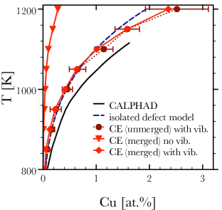
Figure 3: (color online) Phase boundaries of Fe-rich Fe_1-xCu_x alloys. First-principles results of 10 CEs and one MC without (triangles, red line) and with vibrational free energies, utilizing temperature dependent ECIs (diamonds, red line) and merged figure sets; Shown are results averaged over 10 corresponding MCs (red circles, dotted line) including error bars, and results of a first-principles calculation with single-atom and pairwise Cu-defects (blue dashed line)  Reith and Podloucky (2009). Semi-empirical CALPHAD data Franke and Neuschütz (1994) are indicated as a solid black line .

Figure 3 presents the phase boundaries at the Fe-rich side. By comparing the results without and with contributions from the vibrational free energies the very striking difference is obvious: without $F_{\text{vib},\text{DFT}}(\sigma,T)$ the solubility is much too small compared to semi-empirical CALPHAD data Franke and Neuschütz (1994). Obviously, vibrational entropies are responsible for this effect. A comparison of the CE + MC derived phase boundaries to the isolated defect model Reith and Podloucky (2009) reveals a perfect agreement at lower temperatures. But at higher temperatures larger defect clusters of Cu atoms enter the stage, as demonstrated by Fig. 4. The CE + MC simulation at 1000 K finds most of the dissolved Cu as single-atom and pair-wise defects mirroring the isolated defect model. Increasing the temperature to 1200 K, CE + MC produces a substantial percentage of larger sized Cu-clusters thus demonstrating the concentration dependence of this approach and the deficit of the isolated defect model.

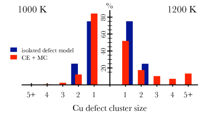
Figure 4: (color online) Distribution of Cu cluster sizes given as percentage of the total number of dissolved Cu atoms for the point defect model Reith and Podloucky (2009) (blue bars) and the temperature dependent CE + MC calculation (red bars) with the merged figure set strategy (see text).

Summarized, we have presented a combination of CE and temperature dependent properties in terms of vibrational free energies. With the averaged CEs (Eq. 5) a single set of ECIs $\bar{J}_{\text{f}}(T)$ within a merged figure set $\bar{\mathbb{F}}(T)$ has been derived by which one can further study, for example, the growth kinetics of precipitates. The presented concept for a temperature dependent CE is in principle straightforward and also feasible, in particular if the strategy of the merged figure sets is utilized. Clearly, there is still need for future improvement: in particular, one should aim at reducing the number of figures in the merged figure set in order to reduce the computational cost of MC simulations. In the case of Fe-rich Fe_1-xCu_x we have demonstrated that the inclusion of vibrational free energies in the CE+MC simulations is absolutely vital: only then are realistic values obtained for the solubility of Cu in an bcc-Fe matrix, and only then do our results agree with experimental data. The main physics behind this surprisingly large solubility of Cu in Fe is effectively described by a concentration and temperature dependent and purely first-principles approach which also includes vibrational free energies.

Work at the University of Vienna was supported by the Austrian Science Fund (FWF) within the Special Research Program VICOM (Vienna Computational Materials Laboratory, project no. F4110). Calculations were done on the Vienna Scientific Cluster (VSC) under project no. 70134.

References

- Sanchez et al. (1984) J. Sanchez, F. Ducastelle, and D. Gratias, Physcia A 128, 334 (1984).
- Ferreira et al. (1989) L. G. Ferreira, S.-H. Wei, and A. Zunger, Phys. Rev. B 40, 3197 (1989).
- Müller (2003) S. Müller, Journal of Physics: Condensed Matter 15, R1429 (2003).
- Lerch et al. (2009) D. Lerch, O. Wieckhorst, G. Hart, R. Forcade, and S. Müller, Modelling Simul. Mater. Sci. Eng. 17, 055003 (2009).
- Lu et al. (1991) Z. W. Lu, S.-H. Wei, A. Zunger, S. Frota-Pessoa, and L. G. Ferreira, Phys. Rev. B 44, 512 (1991).
- van de Walle and Ceder (2002) A. van de Walle and G. Ceder, Journal of Phase Equilibria 23, 348 (2002).
- Hart et al. (2005) G. L. W. Hart, V. Blum, M. J. Walorski, and A. Zunger, Nature Materials 4, 391 (2005).
- Blum et al. (2005) V. Blum, G. L. W. Hart, M. J. Walorski, and A. Zunger, Phys. Rev. B 72, 165113 (2005).
- Kerscher et al. (2011) T. C. Kerscher, S. Müller, Q. O. Snell, and G. L. W. Hart, in 2011 International Parallel and Distributed Processing Symposium (2011) p. 1234.
- Garbulsky and Ceder (1994) G. D. Garbulsky and G. Ceder, Phys. Rev. B 49, 6327 (1994).
- Craievich and Sanchez (1997) P. J. Craievich and J. M. Sanchez, Comp. Mat. Science 8, 92 (1997).
- Stöhr et al. (2009) M. Stöhr, R. Podloucky, and S. Müller, J. Phys. Cond. Mat. 21, 134017 (2009).
- Franke and Neuschütz (1994) P. Franke and D. Neuschütz, Cu-Fe, edited by P. Franke and D. Neuschütz, Landolt-Börnstein New Series, Vol. IV/19B3 (Springer Verlag, Berlin, 1994).
- Reith and Podloucky (2009) D. Reith and R. Podloucky, Physical Review B 80, 054108 (2009).
- Walle and Ceder (2002) A. V. D. Walle and G. Ceder, Rev. Mod. Phys. 74, 11 (2002).
- Ozoliņš et al. (1998) V. Ozoliņš, C. Wolverton, and A. Zunger, Phys. Rev. B 58, R5897 (1998).
- Yuge et al. (2008) K. Yuge, A. Seko, Y. Koyama, F. Oba, and I. Tanaka, Physical Review B 77, 094121 (2008).
- Kresse and Joubert (1999) G. Kresse and D. Joubert, Physical Review B 59, 1758 (1999).
- Kresse and Furthmüller (1996) G. Kresse and J. Furthmüller, Physical Review B 54, 11169 (1996).
- Blöchl (1994) P. Blöchl, Physical Review B 50, 17953 (1994).
- Perdew et al. (1996) J. P. Perdew, K. Burke, and M. Ernzerhof, Physical Review Letters 77, 3865 (1996).
- Alfè (2009) D. Alfè, Comp. Phys. Commun. 180, 2622 (2009).
- Seko et al. (2009) A. Seko, Y. Koyama, and I. Tanaka, Physical Review B 80, 165122 (2009).
- Liu et al. (2005) J. Z. Liu, A. van de Walle, G. Ghosh, and M. Asta, Physical Review B 72, 144109 (2005).
- Souvatzis et al. (2008) P. Souvatzis, O. Eriksson, M. Katsnelson, and S. Rudin, Physical Review Letters, 095901 (2008).