General relations for quantum gases in two and three
dimensions: Two-component fermions

Abstract

We derive exact general relations between various observables for $N$ spin-1/2 fermions with zero-range or short-range interactions, in continuous space or on a lattice, in two or three dimensions, in an arbitrary external potential. Some of our results generalize known relations between the large-momentum behavior of the momentum distribution, the short-distance behaviors of the pair distribution function and of the one-body density matrix, the norm of the regular part of the wavefunction, the derivative of the energy with respect to the scattering length or to time, and the interaction energy (in the case of finite-range interactions). The expression relating the energy to a functional of the momentum distribution is also generalized. Moreover, expressions are found (in terms of the regular part of the wavefunction) for the derivative of the energy with respect to the effective range $r_{e}$ in $3D$, and to the effective range squared in $2D$. They express the fact that the leading corrections to the eigenenergies due to a finite interaction-range are linear in the effective range in $3D$ (and in its square in $2D$) with model-independent coefficients. There are subtleties in the validity condition of this conclusion, for the $2D$ continuous space (where it is saved by factors that are only logarithmically large in the zero-range limit) and for the $3D$ lattice models (where it applies only for some magic dispersion relations on the lattice, that sufficiently weakly break Galilean invariance and that do not have cusps at the border of the first Brillouin zone; an example of such relations is constructed). Furthermore, the subleading short distance behavior of the pair distribution function and the subleading $1/k^{6}$ tail of the momentum distribution are related to $\partial E/\partial r_{e}$ (or to $\partial E/\partial(r_{e}^{2})$ in $2D$). The second order derivative of the energy with respect to the inverse (or the logarithm in the two-dimensional case) of the scattering length is found to be expressible, for any eigenstate, in terms of the eigenwavefunctions’ regular parts; this implies that, at thermal equilibrium, this second order derivative, taken at fixed entropy, is negative. Applications of the general relations are presented: We compute corrections to exactly solvable two-body and three-body problems and find agreement with available numerics; for the unitary gas in an isotropic harmonic trap, we determine how the finite-$1/a$ and finite range energy corrections vary within each energy ladder (associated to the $SO(2,1)$ dynamical symmetry) and we deduce the frequency shift and the collapse time of the breathing mode; for the bulk unitary gas, we compare to fixed-node Monte Carlo data, and we estimate the deviation from the Bertsch parameter due to the finite interaction range in typical experiments.

I General introduction

The experimental breakthroughs of 1995 having led to the first realization of a Bose-Einstein condensate in an atomic vapor Anderson et al. (1995); Bradley et al. (1995); Davis et al. (1995) have opened the era of experimental studies of ultracold gases with non-negligible or even strong interactions, in dimension lower than or equal to three Bloch et al. (2008); Giorgini et al. (2008); Hou (2001, 2004); Var (2007). In these systems, the thermal de Broglie wavelength and the typical distance between atoms are much larger than the range of the interaction potential. This so-called zero-range regime has interesting universal properties: Several quantities such as the thermodynamic functions of the gas depend on the interaction potential only through the scattering length $a$, a length that can be defined in any dimension and that characterizes the low-energy scattering amplitude of two atoms.

This universality property holds for the weakly repulsive Bose gas in three dimensions Lee et al. (1957a) up to the order of expansion in $(na^{3})^{1/2}$ corresponding to Bogoliubov theory Wu (1959); Giuliani and Seiringer (2009), $n$ being the gas density. It also holds for the weakly repulsive Bose gas in two dimensions Schick (1971); Popov (1972); Lieb and Yngvason (2001); Mora and Castin (2003), even at the next order beyond Bogoliubov theory Mora and Castin (2009). For $a$ much larger than the range of the interaction potential, the ground state of $N$ bosons in two dimensions is a universal $N$-body bound state L.W.Bruch and Tjon (1979); Nielsen et al. (1999); Platter et al. (2004); Hammer and Son (2004); Lee (2006). In one dimension, the universality holds for any scattering length, as exemplified by the fact that the Bose gas with zero-range interaction is exactly solvable by the Bethe ansatz both in the repulsive case Lieb and Liniger (1963) and in the attractive case Mc Guire (1964); Castin and Herzog (2001); Calabrese and Caux (2007).

For spin 1/2 fermions, the universality properties are expected to be even stronger. The weakly interacting regimes in $3D$ Lee and Yang (1957); Huang and Yang (1957); Abrikosov and Khalatnikov (1958); Galitskii (1958); Lieb et al. (2005); Seiringer (2006) and in $2D$ Bloom (1975) are universal, as well as for any scattering length in the Bethe-ansatz-solvable $1D$ case Gaudin (1967, 1983). Universality is also expected to hold for an arbitrary scattering length even in $3D$, as was recently tested by experimental studies on the BEC-BCS crossover using a Feshbach resonance, see Var (2007) and Refs. therein and e. g. Partridge et al. (2005, 2006); Thomas et al. (2005); Luo et al. (2007); Luo and Thomas (2009); Stewart et al. (2008); Schirotzek et al. (2008); Riedl et al. (2008); Schirotzek et al. (2009); Nascimbène et al. (2010a, b); Horikoshi et al. (2010); Navon et al. (2010); Ku et al. (2012); Gaebler et al. (2010); Kuhnle et al. (2010, 2011); Stewart et al. (2010), and in agreement with unbiased Quantum Monte Carlo calculations Bulgac et al. (2006); Burovski et al. (2006a); Juillet (2007); Bulgac et al. (2008); Burovski et al. (2008); Chang (2008); Van Houcke et al. (2012); and in $2D$, a similar universal crossover from BEC to BCS is expected when the parameter $\ln(k_{F}a)$ [where $k_{F}$ is the Fermi momentum] varies from $-\infty$ to $+\infty$ Petrov et al. (2003); Miyake (1983); Randeria et al. (1989); Drechsler and Zwerger (1992); Brodsky et al. (2006); Bertaina and Giorgini (2011); Feld et al. (2011); Vogt et al. (2012). Mathematically, results on universality were obtained for the $N$-body problem in $2D$ Dell’Antonio et al. (1994). In $3D$, mathematical results were obtained for the $3$-body problem (see, e.g., Minlos and Faddeev (1961a, b); Vugalter and Zhislin (1982); Shermatov (2003); Albeverio et al. (1981)). The universality for the fermionic equal-mass $N$-body problem in $3D$ remains mathematically unproven .

Universality is also expected for mixtures in $2D$ Petrov et al. (2007); Brodsky et al. (2006); Pricoupenko and Pedri (2010), and in $3D$ for Fermi-Fermi mixtures below a critical mass ratio Efimov (1973); Petrov et al. (2007); Baranov et al. (2008); Castin et al. (2010). Above a critical mass ratio, the Efimov effect takes place, as it also takes place for bosons Efimov (1970); Braaten and Hammer (2006). In this case, the three-body problem depends on a single additional parameter, the three-body parameter. The Efimov physics is presently under active experimental investigation Kraemer et al. (2006); Zaccanti et al. (2009); Gross et al. (2009); Efimov (2009); Pollack et al. (2009); Gross et al. (2010); Lompe et al. (2010). It is not the subject of this paper (see Werner and Castin (a)).

In the zero-range regime, it is intuitive that the short-range or high-momenta properties of the gas are dominated by two-body physics. For example the pair distribution function $g^{(2)}(\mathbf{r}_{12})$ of particles at distances $r_{12}$ much smaller than the de Broglie wavelength is expected to be proportional to the modulus squared of the zero-energy two-body scattering-state wavefunction $\phi(\mathbf{r}_{12})$, with a proportionality factor $\Lambda_{g}$ depending on the many-body state of the gas. Similarly the tail of the momentum distribution $n(\mathbf{k})$, at wavevectors much larger than the inverse de Broglie wavelength, is expected to be proportional to the modulus squared of the Fourier component $\tilde{\phi}(\mathbf{k})$ of the zero-energy scattering-state wavefunction, with a proportionality factor $\Lambda_{n}$ depending on the many-body state of the gas: Whereas two colliding atoms in the gas have a center of mass wavevector of the order of the inverse de Broglie wavelength, their relative wavevector can access much larger values, up to the inverse of the interaction range, simply because the interaction potential has a width in the space of relative momenta of the order of the inverse of its range in real space.

For these intuitive reasons, and with the notable exception of one-dimensional systems, one expects that the mean interaction energy $E_{\rm int}$ of the gas, being sensitive to the shape of $g^{(2)}$ at distances of the order of the interaction range, is not universal, but diverges in the zero-range limit; one also expects that, apart from the $1D$ case, the mean kinetic energy, being dominated by the tail of the momentum distribution, is not universal and diverges in the zero-range limit, a well known fact in the context of Bogoliubov theory for Bose gases and of BCS theory for Fermi gases. Since the total energy of the gas is universal, and $E_{\rm int}$ is proportional to $\Lambda_{g}$ while $E_{\rm kin}$ is proportional to $\Lambda_{n}$, one expects that there exists a simple relation between $\Lambda_{g}$ and $\Lambda_{n}$.

The precise link between the pair distribution function, the tail of the momentum distribution and the energy of the gas was first established for one-dimensional systems. In Lieb and Liniger (1963) the value of the pair distribution function for $r_{12}=0$ was expressed in terms of the derivative of the gas energy with respect to the one-dimensional scattering length, thanks to the Hellmann-Feynman theorem. In Olshanii and Dunjko (2003) the tail of $n(k)$ was also related to this derivative of the energy, by using a simple and general property of the Fourier transform of a function having discontinuous derivatives in isolated points.

In three dimensions, results in these directions were first obtained for weakly interacting gases. For the weakly interacting Bose gas, Bogoliubov theory contains the expected properties, in particular on the short distance behavior of the pair distribution function Lee et al. (1957b); Holzmann and Castin (1999); Naraschewki and Glauber (1999) and the fact that the momentum distribution has a slowly decreasing tail. For the weakly interacting spin-1/2 Fermi gas, it was shown that the BCS anomalous average (or pairing field) $\langle\hat{\psi}_{\uparrow}(\mathbf{r}_{1})\hat{\psi}_{\downarrow}(\mathbf{r}_{2})\rangle$ behaves at short distances as the zero-energy two-body scattering wavefunction $\phi(\mathbf{r}_{12})$ Bruun et al. (1999), resulting in a $g^{(2)}$ function indeed proportional to $|\phi(\mathbf{r}_{12})|^{2}$ at short distances. It was however understood later that the corresponding proportionality factor $\Lambda_{g}$ predicted by BCS theory is incorrect Castin and Carusotto (2004), e.g. at zero temperature the BCS prediction drops exponentially with $1/a$ in the non-interacting limit $a\to 0^{-}$, whereas the correct result drops as a power law in $a$.

More recently, in a series of two articles Tan (2008a, b), explicit expressions for the proportionality factors $\Lambda_{g}$ and $\Lambda_{n}$ were obtained in terms of the derivative of the gas energy with respect to the inverse scattering length, for a spin-1/2 interacting Fermi gas in three dimensions, for an arbitrary value of the scattering length, that is, not restricting to the weakly interacting limit. Later on, these results were rederived in Braaten and Platter (2008); Braaten et al. (2008); Zhang and Leggett (2009), and also in Werner et al. (2009) with very elementary methods building on the aforementioned intuition that $g^{(2)}(\mathbf{r}_{12})\propto|\phi(\mathbf{r}_{12})|^{2}$ at short distances and $n(\mathbf{k})\propto|\tilde{\phi}(\mathbf{k})|^{2}$ at large momenta. These relations were tested by numerical four-body calculations Blume and Daily (2009). An explicit relation between $\Lambda_{g}$ and the interaction energy was derived in Zhang and Leggett (2009). Another fundamental relation discovered in Tan (2008a) and recently generalized in Tan (a); Combescot et al. (2009a) to fermions in $2D$, expresses the total energy as a functional of the momentum distribution and the spatial density.

II Contents

Here we derive generalizations of the relations of Lieb and Liniger (1963); Olshanii and Dunjko (2003); Tan (2008a, b); Zhang and Leggett (2009); Tan (a); Combescot et al. (2009a) to two dimensional gases, and to the case of a small but non-zero interaction range (both on a lattice and in continuous space). We also find entirely new results for the first order derivative of the energy with respect to the effective range, as well as for the second order derivative with respect to the scattering length. We shall also include rederivations of known relations using our elementary methods. We treat in detail the case of spin-1/2 fermions, with equal masses in the two spin states, both in three dimensions and in two dimensions. The discussion of spinless bosons and arbitrary mixtures is deferred to another article, as it may involve the Efimov effect in three dimensions Werner and Castin (b).

This article is organized as follows. Models, notations and some basic properties are introduced in Section III. Relations for zero-range interactions are summarized in Table 2 and derived for pure states in Section IV. We then consider lattice models (Tab. 3 and Sec. V) and finite-range models in continuous space (Tab. 4 and Sec. VI). In Section VII we derive a model-independent expression for the correction to the energy due to a finite range or a finite effective range of the interaction, and we relate this energy correction to the subleading short distance behavior of the pair distribution function and to the coefficient of the $1/k^{6}$ subleading tail of the momentum distribution (see Tab. 5). The case of general statistical mixtures of pure states or of stationary states is discussed in Sec. VIII, and the case of thermodynamic equilibrium states in Sec. IX. Finally we present applications of the general relations: For two particles and three particles in harmonic traps we compute corrections to exactly solvable cases (Sec. X.1 and Sec. X.2). For the unitary gas trapped in an isotropic harmonic potential, we determine how the equidistance between levels within a given energy ladder (resulting from the $SO(2,1)$ dynamical symmetry) is affected by finite $1/a$ and finite range corrections, which leads to a frequency shift and a collapse of the breathing mode of the zero-temperature gas (Sec. X.3). For the bulk unitary gas, we check that general relations are satisfied by existing fixed-node Monte Carlo data Astrakharchik et al. (2004, 2005); Lobo et al. (2006) for correlation functions of the unitary gas (Sec. X.4). We quantify the finite range corrections to the unitary gas energy in typical experiments, which is required for precise measurements of its equation of state (Sec. X.5). We conclude in Section XI.

Three dimensions		Two dimensions
$\displaystyle\psi(\mathbf{r}_{1},\ldots,\mathbf{r}_{N})\underset{r_{ij}\to 0}{=}\left(\frac{1}{r_{ij}}-\frac{1}{a}\right)\,A_{ij}\left(\mathbf{R}_{ij},(\mathbf{r}_{k})_{k\neq i,j}\right)+O(r_{ij})\$	(1a)	$\displaystyle\psi(\mathbf{r}_{1},\ldots,\mathbf{r}_{N})\underset{r_{ij}\to 0}{=}\ln(r_{ij}/a)\,A_{ij}\left(\mathbf{R}_{ij},(\mathbf{r}_{k})_{k\neq i,j}\right)+O(r_{ij})\$	(1b)
$\displaystyle(A^{(1)},A^{(2)})\equiv\sum_{i<j}\int\Big{(}\prod_{k\neq i,j}d^{d}\!r_{k}\Big{)}d^{d}\!R_{ij}A^{(1)*}_{ij}(\mathbf{R}_{ij},(\mathbf{r}_{k})_{k\neq i,j})A^{(2)}_{ij}(\mathbf{R}_{ij},(\mathbf{r}_{k})_{k\neq i,j})$			(2)
$\displaystyle(A^{(1)},\mathcal{H}A^{(2)})\equiv\sum_{i<j}\int\Big{(}\prod_{k\neq i,j}d^{d}\!r_{k}\Big{)}d^{d}\!R_{ij}A^{(1)*}_{ij}(\mathbf{R}_{ij},(\mathbf{r}_{k})_{k\neq i,j})\mathcal{H}_{ij}A^{(2)}_{ij}(\mathbf{R}_{ij},(\mathbf{r}_{k})_{k\neq i,j})$			(3)

Table 1: Notation for the regular part $A$ of the $N$-body wavefunction appearing in the contact conditions (first line, with $\mathbf{R}_{ij}=(\mathbf{r}_{i}+\mathbf{r}_{j})/2$ fixed), for the scalar product between such regular parts (second line) and for corresponding matrix elements of operators $\mathcal{H}_{ij}$ acting on $\mathbf{R}_{ij}$ and on the $\mathbf{r}_{k}$, $k\neq i,j$ (third line).

III Models, notations, and basic properties

We now introduce the three models used in this work to account for interparticle interactions and associated notations, together with some basic properties to be used in some of the derivations.

For a fixed number $N_{\sigma}$ of fermions in each spin state $\sigma=\uparrow,\downarrow$, one can consider that particles $1,\ldots,N_{\uparrow}$ have a spin $\uparrow$ and particles $N_{\uparrow}+1,\ldots,N_{\uparrow}+N_{\downarrow}=N$ have a spin $\downarrow$, so that the wavefunction $\psi(\mathbf{r}_{1},\ldots,\mathbf{r}_{N})$ (normalized to unity) changes sign when one exchanges the positions of two particles having the same spin .

III.1 Zero-range model

In this well-known model (see e.g. Albeverio et al. (1988); Castin (2001); Petrov et al. (2005); Efimov (1970); Pricoupenko and Olshanii (2007); Braaten and Hammer (2006); Castin (2007); Werner (2008a) and refs. therein) the interaction potential is replaced by boundary conditions on the $N$-body wavefunction: For any pair of particles $i\neq j$, there exists a function $A_{ij}$, hereafter called regular part of $\psi$, such that [Tab. I, Eq. (1a)] holds in the $3D$ case and [Tab. I, Eq. (1b)] holds in the $2D$ case, where the limit of vanishing distance $r_{ij}$ between particles $i$ and $j$ is taken for a fixed position of their center of mass $\mathbf{R}_{ij}=(\mathbf{r}_{i}+\mathbf{r}_{j})/2$ and fixed positions of the remaining particles $(\mathbf{r}_{k})_{k\neq i,j}$ different from $\mathbf{R}_{ij}$. Fermionic symmetry of course imposes $A_{ij}=0$ if particles $i$ and $j$ have the same spin. When none of the $\mathbf{r}_{i}$’s coincide, there is no interaction potential and Schrödinger’s equation reads $H\,\psi(\mathbf{r}_{1},\ldots,\mathbf{r}_{N})=E\,\psi(\mathbf{r}_{1},\ldots,\mathbf{r}_{N})$ with $\displaystyle H=-\frac{\hbar^{2}}{2m}\sum_{i=1}^{N}\Delta_{\mathbf{r}_{i}}+H_{\rm trap}$, where $m$ is the atomic mass and the trapping potential energy is

$$H_{\rm trap}\equiv\sum_{i=1}^{N}U(\mathbf{r}_{i}),$$ (1)

$U$ being an external trapping potential. The crucial difference between the Hamiltonian $H$ and the non-interacting Hamiltonian is the boundary condition [Tab. I, Eqs. (1a,1b)].

III.2 Lattice models

These models are used for quantum Monte Carlo calculations Bulgac et al. (2006); Burovski et al. (2006a, b); Juillet (2007); Chang (2008); Bulgac et al. (2008). They can also be convenient for analytics, as used in Mora and Castin (2003); Pricoupenko and Castin (2007a); Werner et al. (2009); Mora and Castin (2009) and in this work. Particles live on a lattice, i. e. the coordinates are integer multiples of the lattice spacing $b$. The Hamiltonian is

$$H=H_{\rm kin}+H_{\rm int}+H_{\rm trap}$$ (2)

with, in first quantization, the kinetic energy

$$H_{\rm kin}=-\frac{\hbar^{2}}{2m}\sum_{i=1}^{N}\Delta_{\mathbf{r}_{i}},$$ (3)

the interaction energy

$$H_{\rm int}=g_{0}\sum_{i<j}\delta_{\mathbf{r}_{i},\mathbf{r}_{j}}b^{-d},$$ (4)

and the trapping potential energy defined by (1); i.e. in second quantization

$$H_{\rm kin} = \sum_{\sigma}\int_{D}\frac{d^{d}k}{(2\pi)^{d}}\,\epsilon_{\mathbf{k}}c_{\sigma}^{\dagger}(\mathbf{k})c_{\sigma}(\mathbf{k})$$ (5)

$$H_{\rm int} = g_{0}\sum_{\mathbf{r}}b^{d}(\psi^{\dagger}_{\uparrow}\psi^{\dagger}_{\downarrow}\psi_{\downarrow}\psi_{\uparrow})(\mathbf{r})$$ (6)

$$H_{\rm trap} = \sum_{\mathbf{r},\sigma}b^{d}U(\mathbf{r})(\psi_{\sigma}^{\dagger}\psi_{\sigma})(\mathbf{r}).$$ (7)

Here $d$ is the space dimension, $\epsilon_{\mathbf{k}}$ is the dispersion relation, $\hat{\psi}$ obeys discrete anticommutation relations $\{\hat{\psi}_{\sigma}(\mathbf{r}),\hat{\psi}^{\dagger}_{\sigma^{\prime}}(\mathbf{r}^{\prime})\}=b^{-d}\delta_{\mathbf{r}\mathbf{r}^{\prime}}\delta_{\sigma\sigma^{\prime}}$. The operator $c_{\sigma}^{\dagger}(\mathbf{k})$ creates a particle in the plane wave state $|\mathbf{k}\rangle$ defined by $\langle\mathbf{r}|\mathbf{k}\rangle=e^{i\mathbf{k}\cdot\mathbf{r}}$ for any $\mathbf{k}$ belonging to the first Brillouin zone $D=\left(-\frac{\pi}{b},\frac{\pi}{b}\right]^{d}$. The corresponding anticommutation relations are $\{c_{\sigma}(\mathbf{k}),c^{\dagger}_{\sigma^{\prime}}(\mathbf{k}^{\prime})\}=(2\pi)^{d}\delta_{\sigma\sigma^{\prime}}\delta(\mathbf{k}-\mathbf{k}^{\prime})$ if $\mathbf{k}$ and $\mathbf{k}^{\prime}$ are both in the first Brillouin zone . The operator $\Delta$ in (3) is the lattice version of the Laplacian defined by $-\frac{\hbar^{2}}{2m}\langle\mathbf{r}|\Delta_{\mathbf{r}}|\mathbf{k}\rangle\equiv\epsilon_{\mathbf{k}}\langle\mathbf{r}|\mathbf{k}\rangle$. The simplest choice for the dispersion relation is $\displaystyle\epsilon_{\mathbf{k}}=\frac{\hbar^{2}k^{2}}{2m}$ Mora and Castin (2003); Juillet (2007); Pricoupenko and Castin (2007a); Mora and Castin (2009); Chang (2008). Another choice, used in Burovski et al. (2006a, b), is the dispersion relation of the Hubbard model: $\displaystyle\epsilon_{\mathbf{k}}=\frac{\hbar^{2}}{mb^{2}}\sum_{i=1}^{d}\left[1-\cos(k_{i}b)\right]$. More generally, what follows applies to any $\epsilon_{\mathbf{k}}$ such that $\displaystyle\epsilon_{\mathbf{k}}\underset{b\to 0}{\rightarrow}\frac{\hbar^{2}k^{2}}{2m}$ sufficiently rapidly and $\epsilon_{-\mathbf{k}}=\epsilon_{\mathbf{k}}$.

A key quantity is the zero-energy scattering state $\phi(\mathbf{r})$, defined by the two-body Schrödinger equation (with the center of mass at rest)

$$\left(-\frac{\hbar^{2}}{m}\,\Delta_{\mathbf{r}}+g_{0}\frac{\delta_{\mathbf{r},\mathbf{0}}}{b^{d}}\right)\phi(\mathbf{r})=0$$ (8)

and by the normalization conditions

$$\phi(\mathbf{r}) \underset{r\gg b}{\simeq} \frac{1}{r}-\frac{1}{a}\ \ \ {\rm in}\ 3D$$ (9)

$$\phi(\mathbf{r}) \underset{r\gg b}{\simeq} \ln(r/a)\ \ \ {\rm in}\ 2D.$$ (10)

A two-body analysis, detailed in Appendix A, yields the relation between the scattering length and the bare coupling constant $g_{0}$, in three and two dimensions:

$$\frac{1}{g_{0}}\stackrel{{\scriptstyle 3D}}{{=}}\frac{m}{4\pi\hbar^{2}a}\!-\!\!\int_{D}\!\!\frac{d^{3}k}{(2\pi)^{3}}\frac{1}{2\epsilon_{\mathbf{k}}}$$ (11)

$$\frac{1}{g_{0}}\stackrel{{\scriptstyle 2D}}{{=}}\lim_{q\to 0}\left[-\frac{m}{2\pi\hbar^{2}}\ln(\frac{aqe^{\gamma}}{2})\!+\!\!\int_{D}\!\!\frac{d^{2}k}{(2\pi)^{2}}\mathcal{P}\frac{1}{2(\epsilon_{\mathbf{q}}-\epsilon_{\mathbf{k}})}\right]$$ (12)

where $\gamma=0.577216\ldots$ is Euler’s constant and $\mathcal{P}$ is the principal value. This implies that (for constant $b$):

$$\frac{d(1/g_{0})}{d(1/a)}=\frac{m}{4\pi\hbar^{2}} \ \ \ {\rm in}\ 3D$$ (13)

$$\frac{d(1/g_{0})}{d(\ln a)}=-\frac{m}{2\pi\hbar^{2}} \ \ \ {\rm in}\ 2D.$$ (14)

Another useful property derived in Appendix A is

$$\phi(\mathbf{0}) = -\frac{4\pi\hbar^{2}}{mg_{0}}\ \ \ {\rm in}\ 3D$$ (15)

$$\phi(\mathbf{0}) = \frac{2\pi\hbar^{2}}{mg_{0}}\ \ \ {\rm in}\ 2D,$$ (16)

which, together with (13,14), gives

$$|\phi(\mathbf{0})|^{2} = \frac{4\pi\hbar^{2}}{m}\frac{d(-1/a)}{dg_{0}}\ \ \ {\rm in}\ 3D$$ (17)

$$|\phi(\mathbf{0})|^{2} = \frac{2\pi\hbar^{2}}{m}\frac{d(\ln a)}{dg_{0}}\ \ \ {\rm in}\ 2D.$$ (18)

In the zero-range limit ($b\to 0$ with $g_{0}$ adjusted in such a way that $a$ remains constant), it is expected that the spectrum of the lattice model converges to the one of the zero-range model, as explicitly checked for three particles in Pricoupenko and Castin (2007a), and that any eigenfunction $\psi(\mathbf{r}_{1},\dots,\mathbf{r}_{N})$ of the lattice model tends to the corresponding eigenfunction of the zero-range model provided all interparticle distances remain much larger than $b$. For any stationary state, let us denote by $1/k_{\rm typ}$ the typical length-scale on which the zero-range model’s wavefunction varies: e.g. for the lowest eigenstates, this is on the order of the mean interparticle distance, or on the order of $a$ in the regime where $a$ is small and positive and dimers are formed. The zero-range limit is then reached if $k_{\rm typ}b\ll 1$. This notion of typical wavevector $k_{\rm typ}$ can also be applied to the case of a thermal equilibrium state, since most significantly populated eigenstates then have a $k_{\rm typ}$ on the same order; it is then expected that the thermodynamic potentials converge to the ones of the zero-range model when $b\to 0$, and that this limit is reached provided $k_{\rm typ}b\ll 1$. For the homogeneous gas, defining a thermal wavevector $k_{T}$ by $\hbar^{2}k_{T}^{2}/(2m)=k_{B}\,T$, we have $k_{\rm typ}\sim\max(k_{F},k_{T})$ for $a<0$ and $k_{\rm typ}\sim\max(k_{F},k_{T},1/a)$ for $a>0$.

For lattice models, it will prove convenient to define the regular part $A$ by

$$\psi(\mathbf{r}_{1},\ldots,\mathbf{r}_{i}=\mathbf{R}_{ij},\ldots,\mathbf{r}_{j}=\mathbf{R}_{ij},\ldots,\mathbf{r}_{N})=\phi(\mathbf{0})\\ \times A_{ij}(\mathbf{R}_{ij},(\mathbf{r}_{k})_{k\neq i,j}).$$ (19)

In the zero-range regime $k_{\rm typ}b\ll 1$, when the distance $r_{ij}$ between two particles of opposite spin is $\ll 1/k_{\rm typ}$ while all the other interparticle distances are much larger than $b$ and than $r_{ij}$, the many-body wavefunction is proportional to $\phi(\mathbf{r}_{j}-\mathbf{r}_{i})$, with a proportionality constant given by (19):

$$\psi(\mathbf{r}_{1},\ldots,\mathbf{r}_{N})\simeq\phi(\mathbf{r}_{j}-\mathbf{r}_{i})\,A_{ij}(\mathbf{R}_{ij},(\mathbf{r}_{k})_{k\neq i,j})$$ (20)

where $\mathbf{R}_{ij}=(\mathbf{r}_{i}+\mathbf{r}_{j})/2$. If moreover $r_{ij}\gg b$, $\phi$ can be replaced by its asymptotic form (9,10); since the contact conditions [Tab. I, Eqs. (1a,1b)] of the zero-range model must be recovered, we see that the lattice model’s regular part tends to the zero-range model’s regular part in the zero-range limit.

III.3 Finite-range continuous-space models

Such models are used in numerical few-body correlated Gaussian and many-body fixed-node Monte Carlo calculations (see e. g. Carlson et al. (2003); Astrakharchik et al. (2004); Blume et al. (2007); von Stecher et al. (2008); Blume and Daily (2009); Giorgini et al. (2008); Bertaina and Giorgini (2011) and refs. therein). They are also relevant to neutron matter Gezerlis and Carlson (2008). The Hamiltonian reads

$$H=H_{0}+\sum_{i=1}^{N_{\uparrow}}\sum_{j=N_{\uparrow}+1}^{N}\,V(r_{ij}),$$ (21)

$H_{0}$ being defined by (3) where $\Delta_{\mathbf{r}_{i}}$ now stands for the usual Laplacian, and $V(r)$ is an interaction potential between particles of opposite spin, which vanishes for $r>b$ or at least decays quickly enough for $r\gg b$. The two-body zero-energy scattering state $\phi(r)$ is again defined by the Schrödinger equation $-(\hbar^{2}/m)\Delta_{\mathbf{r}}\phi+V(r)\phi=0$ and the boundary condition (9) or (10). The zero-range regime is again reached for $k_{\rm typ}b\ll 1$ with $k_{\rm typ}$ the typical relative wavevector . Equation (20) again holds in the zero-range regime, where $A$ now simply stands for the zero-range model’s regular part.

IV Relations in the zero-range limit

Three dimensions		Two dimensions
$C\equiv{\displaystyle\lim_{k\to+\infty}}k^{4}n_{\sigma}(\mathbf{k})$			(1)
$\displaystyle C=(4\pi)^{2}\ (A,A)$	(2a)	$\displaystyle C=(2\pi)^{2}\,(A,A)$	(2b)
$\displaystyle\int d^{3}R\,g_{\uparrow\downarrow}^{(2)}\left(\mathbf{R}+\frac{\mathbf{r}}{2},\mathbf{R}-\frac{\mathbf{r}}{2}\right)\underset{r\to 0}{\sim}\frac{C}{(4\pi)^{2}}\frac{1}{r^{2}}$	(3a)	$\displaystyle\int d^{2}R\,g_{\uparrow\downarrow}^{(2)}\left(\mathbf{R}+\frac{\mathbf{r}}{2},\mathbf{R}-\frac{\mathbf{r}}{2}\right)\underset{r\to 0}{\sim}\frac{C}{(2\pi)^{2}}\ln^{2}r$	(3b)
$\displaystyle\frac{dE}{d(-1/a)}=\frac{\hbar^{2}C}{4\pi m}$	(4a)	$\displaystyle\frac{dE}{d(\ln a)}=\frac{\hbar^{2}C}{2\pi m}$	(4b)
$\displaystyle E-E_{\rm trap}=\frac{\hbar^{2}C}{4\pi ma}$		$\displaystyle E-E_{\rm trap}=\lim_{\Lambda\to\infty}\left[-\frac{\hbar^{2}C}{2\pi m}\ln\left(\frac{a\Lambda e^{\gamma}}{2}\right)\right.$
$\displaystyle+\sum_{\sigma}\int\frac{d^{3}\!k}{(2\pi)^{3}}\frac{\hbar^{2}k^{2}}{2m}\left[n_{\sigma}(\mathbf{k})-\frac{C}{k^{4}}\right]$	(5a)	$\displaystyle+\sum_{\sigma}\left.\int_{k<\Lambda}\frac{d^{2}\!k}{(2\pi)^{2}}\frac{\hbar^{2}k^{2}}{2m}n_{\sigma}(\mathbf{k})\right]$	(5b)
$\displaystyle\int d^{3}R\,g_{\sigma\sigma}^{(1)}\left(\mathbf{R}+\frac{\mathbf{r}}{2},\mathbf{R}-\frac{\mathbf{r}}{2}\right)\underset{r\to 0}{=}N_{\sigma}-\frac{C}{8\pi}\,r+O(r^{2})\ \ \$	(6a)	$\displaystyle\int d^{2}R\,g_{\sigma\sigma}^{(1)}\left(\mathbf{R}+\frac{\mathbf{r}}{2},\mathbf{R}-\frac{\mathbf{r}}{2}\right)\underset{r\to 0}{=}N_{\sigma}+\frac{C}{4\pi}\,r^{2}\ln r+O(r^{2})\ \ \$	(6b)
$\displaystyle\frac{1}{3}\sum_{i=1}^{3}\sum_{\sigma}\int d^{3}R\,g_{\sigma\sigma}^{(1)}\left(\mathbf{R}+\frac{r{\bf u_{i}}}{2},\mathbf{R}-\frac{r{\bf u_{i}}}{2}\right)\underset{r\to 0}{=}N$		$\displaystyle\frac{1}{2}\sum_{i=1}^{2}\sum_{\sigma}\int d^{2}R\,g_{\sigma\sigma}^{(1)}\left(\mathbf{R}+\frac{r{\bf u_{i}}}{2},\mathbf{R}-\frac{r{\bf u_{i}}}{2}\right)\underset{r\to 0}{=}N$
$\displaystyle-\frac{C}{4\pi}r-\frac{m}{3\hbar^{2}}\left(E-E_{\rm trap}-\frac{\hbar^{2}C}{4\pi ma}\right)r^{2}+o(r^{2})$	(7a)	$\displaystyle+\frac{C}{4\pi}r^{2}\left[\ln\left(\frac{r}{a}\right)-1\right]-\frac{m}{2\hbar^{2}}\left(E-E_{\rm trap}\right)r^{2}+o(r^{2})$	(7b)
$\displaystyle\frac{1}{2}\frac{d^{2}E_{n}}{d(-1/a)^{2}}=\left(\frac{4\pi\hbar^{2}}{m}\right)^{2}\sum_{n^{\prime},E_{n^{\prime}}\neq E_{n}}\frac{|(A^{(n^{\prime})},A^{(n)})|^{2}}{E_{n}-E_{n^{\prime}}}$	(8a)	$\displaystyle\frac{1}{2}\frac{d^{2}E_{n}}{d(\ln a)^{2}}=\left(\frac{2\pi\hbar^{2}}{m}\right)^{2}\sum_{n^{\prime},E_{n^{\prime}}\neq E_{n}}\frac{|(A^{(n^{\prime})},A^{(n)})|^{2}}{E_{n}-E_{n^{\prime}}}$	(8b)
$\displaystyle\left(\frac{d\bar{E}}{d(-1/a)}\right)_{\!S}=\left(\frac{dF}{d(-1/a)}\right)_{T}=\frac{\hbar^{2}C}{4\pi m}$	(9a)	$\displaystyle\left(\frac{d\bar{E}}{d(\ln a)}\right)_{\!S}=\left(\frac{dF}{d(\ln a)}\right)_{T}=\frac{\hbar^{2}C}{2\pi m}$	(9b)
$\displaystyle\left(\frac{d^{2}F}{d(-1/a)^{2}}\right)_{T}<0$	(10a)	$\displaystyle\left(\frac{d^{2}F}{d(\ln a)^{2}}\right)_{T}<0$	(10b)
$\displaystyle\left(\frac{d^{2}\bar{E}}{d(-1/a)^{2}}\right)_{\!S}<0$	(11a)	$\displaystyle\left(\frac{d^{2}\bar{E}}{d(\ln a)^{2}}\right)_{\!S}<0$	(11b)
$\displaystyle\frac{dE}{dt}=\frac{\hbar^{2}C}{4\pi m}\frac{d(-1/a)}{dt}+\Big{<}\frac{dH_{\rm trap}}{dt}\Big{>}$	(12a)	$\displaystyle\frac{dE}{dt}=\frac{\hbar^{2}C}{2\pi m}\frac{d(\ln a)}{dt}+\Big{<}\frac{dH_{\rm trap}}{dt}\Big{>}$	(12b)

Table 2: Relations for spin-1/2 fermions with zero-range interactions. The definition (1) of $C$, as well as the relations in lines 3, 5, 6 and 7, concern any (non-pathological) statistical mixture of states which satisfy the contact conditions [Tab. I, line 1] (with real wavefunctions for line 7). Line 2 holds for any pure state; here $A$ is the regular part of the wavefunction appearing in the contact condition, and $(A,A)$ is its squared norm (defined in Tab. I). Lines 4 and 8 hold for any stationary state. Lines 9-11 hold at thermal equilibrium in the canonical ensemble. Line 12 holds for any time-dependence of scattering length and trapping potential, and any corresponding time-dependent statistical mixture. Many of the $3D$ relations were originally obtained in Tan (2008a, b) (see text), while the $2D$ relation (5b) was obtained in Combescot et al. (2009a) for the homogeneous system and in Tan (a) (in a different form) for the general case.

We now derive relations for the zero-range model. For some of the derivations we will use a lattice model and then take the zero-range limit. We recall that we derive all relations for pure states in this section, the generalization to statistical mixtures and the discussion of thermal equilibrium being deferred to Sections VIII and IX.

IV.1 Tail of the momentum distribution

In this subsection as well as in the following subsections IV.2, IV.4, IV.5, IV.7, we consider a many-body pure state whose wavefunction $\psi$ satisfies the contact condition [Tab. I, Eqs. (1a,1b)]. We now show that the momentum distribution $n_{\sigma}(\mathbf{k})$ has a $\sigma$-independent tail proportional to $1/k^{4}$, with a coefficient denoted by $C$ [Tab. II, Eq. (1)]. $C$ is usually referred to as the “contact”. We shall also show that $C$ is related by [Tab. II, Eqs. (2a,2b)] to the norm of the regular part $A$ of the wavefunction (defined in Tab. I). In $3D$ these results were obtained in Tan (2008b) . Here the momentum distribution is defined in second quantization by $\displaystyle n_{\sigma}(\mathbf{k})=\langle\hat{n}_{\sigma}(\mathbf{k})\rangle=\langle{c}^{\dagger}_{\sigma}(\mathbf{k}){c}_{\sigma}(\mathbf{k})\rangle$ where ${c}_{\sigma}(\mathbf{k})$ annihilates a particle of spin $\sigma$ in the plane-wave state $|\mathbf{k}\rangle$ defined by $\langle\mathbf{r}|\mathbf{k}\rangle=e^{i\mathbf{k}\cdot\mathbf{r}}$; this corresponds to the normalization

$$\int\frac{d^{d}k}{(2\pi)^{d}}\,n_{\sigma}(\mathbf{k})=N_{\sigma}.$$ (22)

In first quantization,

$$n_{\sigma}(\mathbf{k})=\sum_{i:\sigma}\int\Big{(}\prod_{l\neq i}d^{d}r_{l}\Big{)}\left|\int d^{d}r_{i}e^{-i\mathbf{k}\cdot\mathbf{r}_{i}}\psi(\mathbf{r}_{1},\ldots,\mathbf{r}_{N})\right|^{2}$$ (23)

where the sum is taken over all particles of spin $\sigma$: $i$ runs from $1$ to $N_{\uparrow}$ for $\sigma=\uparrow$, and from $N_{\uparrow}+1$ to $N$ for $\sigma=\downarrow$.

Three dimensions:
The key point is that in the large-$k$ limit, the Fourier transform with respect to $\mathbf{r}_{i}$ is dominated by the contribution of the short-distance divergence coming from the contact condition [Tab. I, Eq. (1a)]:

$$\int d^{3}r_{i}\,e^{-i\mathbf{k}\cdot\mathbf{r}_{i}}\psi(\mathbf{r}_{1},\ldots,\mathbf{r}_{N})\underset{k\to\infty}{\simeq}\int d^{3}r_{i}\,e^{-i\mathbf{k}\cdot\mathbf{r}_{i}}\\ \times\sum_{j,j\neq i}\frac{1}{r_{ij}}A_{ij}(\mathbf{r}_{j},(\mathbf{r}_{l})_{l\neq i,j}).$$ (24)

A similar link between the short-distance singularity of the wavefunction and the tail of its Fourier transform was used to derive exact relations in $1D$ in Olshanii and Dunjko (2003). From $\Delta(1/r)=-4\pi\delta(\mathbf{r})$, we have $\displaystyle\int d^{3}r\,e^{-i\mathbf{k}\cdot\mathbf{r}}\frac{1}{r}=\frac{4\pi}{k^{2}}$, so that

$$\int d^{3}r_{i}\,e^{-i\mathbf{k}\cdot\mathbf{r}_{i}}\psi(\mathbf{r}_{1},\ldots,\mathbf{r}_{N})\underset{k\to\infty}{\simeq}\frac{4\pi}{k^{2}}\sum_{j,j\neq i}e^{-i\mathbf{k}\cdot\mathbf{r}_{j}}\\ \times A_{ij}(\mathbf{r}_{j},(\mathbf{r}_{l})_{l\neq i,j}).$$ (25)

One inserts this into (23) and expands the modulus squared. After spatial integration over all the $\mathbf{r}_{l}$, $l\neq i$, the crossed terms rapidly vanish in the large-$k$ limit, as they are the product of $e^{i\mathbf{k}\cdot(\mathbf{r}_{j}-\mathbf{r}_{j^{\prime}})}$ and of regular functions of $\mathbf{r}_{j}$ and $\mathbf{r}_{j^{\prime}}$ . This yields $n_{\sigma}(\mathbf{k})\underset{k\to\infty}{\sim}C/k^{4}$, with the expression [Tab. II, Eq. (2a)] of $C$ in terms of the norm $(A,A)$ defined in [Tab. I, Eq. (2)].

Two dimensions:
The $2D$ contact condition [Tab. I, Eq. (1b)] now gives

$$\int d^{2}r_{i}\,e^{-i\mathbf{k}\cdot\mathbf{r}_{i}}\psi(\mathbf{r}_{1},\ldots,\mathbf{r}_{N})\underset{k\to\infty}{\simeq}\int d^{2}r_{i}\,e^{-i\mathbf{k}\cdot\mathbf{r}_{i}}\\ \times\sum_{j,j\neq i}\ln(r_{ij})A_{ij}(\mathbf{r}_{j},(\mathbf{r}_{l})_{l\neq i,j}).$$ (26)

From $\Delta(\ln r)=2\pi\delta(\mathbf{r})$, one has $\!\!\displaystyle\int\!\!d^{2}r\,e^{-i\mathbf{k}\cdot\mathbf{r}}\ln r=-\frac{2\pi}{k^{2}}$ and

$$\int d^{2}r_{i}\,e^{-i\mathbf{k}\cdot\mathbf{r}_{i}}\psi(\mathbf{r}_{1},\ldots,\mathbf{r}_{N})\underset{k\to\infty}{\simeq}-\frac{2\pi}{k^{2}}\sum_{j,j\neq i}e^{-i\mathbf{k}\cdot\mathbf{r}_{j}}\\ \times A_{ij}(\mathbf{r}_{j},(\mathbf{r}_{l})_{l\neq i,j}).$$ (27)

As in $3D$ this leads to [Tab. II, Eq. (2b)].

IV.2 Pair distribution function at short distances

The pair distribution function gives the probability density of finding a spin-$\uparrow$ particle at $\mathbf{r}_{\uparrow}$ and a spin-$\downarrow$ particle at $\mathbf{r}_{\downarrow}$: $\displaystyle g_{\uparrow\downarrow}^{(2)}\left(\mathbf{r}_{\uparrow},\mathbf{r}_{\downarrow}\right)=\langle(\hat{\psi}^{\dagger}_{\uparrow}\hat{\psi}_{\uparrow})(\mathbf{r}_{\uparrow})(\hat{\psi}^{\dagger}_{\downarrow}\hat{\psi}_{\downarrow})(\mathbf{r}_{\downarrow})\rangle=\int(\prod_{k=1}^{N}d^{d}r_{k})|\psi(\mathbf{r}_{1},\ldots,\mathbf{r}_{N})|^{2}\sum_{i=1}^{N_{\uparrow}}\sum_{j=N_{\uparrow}+1}^{N}\!\!\!\!\!\!\delta\left(\mathbf{r}_{\uparrow}\!-\!\mathbf{r}_{i}\right)\delta\left(\mathbf{r}_{\downarrow}\!-\!\mathbf{r}_{j}\right)$. We set $\mathbf{r}_{\uparrow,\downarrow}=\mathbf{R}\pm\mathbf{r}/2$ and we integrate over $\mathbf{r}_{i}$ and $\mathbf{r}_{j}$:

$$g_{\uparrow\downarrow}^{(2)}\left(\mathbf{R}+\frac{\mathbf{r}}{2},\mathbf{R}-\frac{\mathbf{r}}{2}\right)=\sum_{i=1}^{N_{\uparrow}}\sum_{j=N_{\uparrow}+1}^{N}\int\Big{(}\prod_{k\neq i,j}d^{d}r_{k}\Big{)}\\ \left|\psi\left(\mathbf{r}_{1},\ldots,\mathbf{r}_{i}=\mathbf{R}+\frac{\mathbf{r}}{2},\ldots,\mathbf{r}_{j}=\mathbf{R}-\frac{\mathbf{r}}{2},\ldots,\mathbf{r}_{N}\right)\right|^{2}$$ (28)

Let us define the spatially integrated pair distribution function 

$$G^{(2)}_{\uparrow\downarrow}(\mathbf{r})\equiv\int d^{d}R\ g_{\uparrow\downarrow}^{(2)}\left(\mathbf{R}+\frac{\mathbf{r}}{2},\mathbf{R}-\frac{\mathbf{r}}{2}\right),$$ (29)

whose small-$r$ singular behavior we will show to be related to $C$ via [Tab. II, Eqs. (3a,3b)].

Three dimensions:
Replacing the wavefunction in (28) by its asymptotic behavior given by the contact condition [Tab. I, Eq. (1a)] immediately yields

$$G^{(2)}_{\uparrow\downarrow}(\mathbf{r})\underset{r\to 0}{\sim}\frac{(A,A)}{r^{2}}.$$ (30)

Expressing $(A,A)$ in terms of $C$ through [Tab. II, Eq. (2a)] finally gives [Tab. II, Eq. (3a)].

In a measurement of all particle positions, the mean total number of pairs of particles of opposite spin which are separated by a distance smaller than $s$ is $N_{\rm pair}(s)=\int_{r<s}d^{d}r\,G^{(2)}_{\uparrow\downarrow}(\mathbf{r})$, so that from [Tab. II, Eq. (3a)]

$$N_{\rm pair}(s)\underset{s\to 0}{\sim}\frac{C}{4\pi}s,$$ (31)

as obtained in Tan (2008a, b).

Two dimensions:
The contact condition [Tab. I, Eq. (1b)] similarly leads to [Tab. II, Eq. (3b)]. After integration over the region $r<s$ this gives

$$N_{\rm pair}(s)\underset{s\to 0}{\sim}\frac{C}{4\pi}s^{2}\ln^{2}s.$$ (32)

IV.3 First order derivative of the energy with respect to the scattering length

The relations [Tab. II, Eqs. (4a,4b)] can be derived straightforwardly using the lattice model, see Sec.V.5. Here we derive them by directly using the zero-range model, which is more involved but also instructive.

Three dimensions:
Let us consider a wavefunction $\psi_{1}$ satisfying the contact condition [Tab. I, Eq. (1a)] for a scattering length $a_{1}$. We denote by $A^{(1)}_{ij}$ the regular part of $\psi_{1}$ appearing in the contact condition [Tab. I, Eq. (1a)]. Similarly, $\psi_{2}$ satisfies the contact condition for a scattering length $a_{2}$ and a regular part $A^{(2)}_{ij}$. Then, as shown in Appendix B using the divergence theorem, the following lemma holds:

$$\langle\psi_{1},H\psi_{2}\rangle-\langle H\psi_{1},\psi_{2}\rangle=\frac{4\pi\hbar^{2}}{m}\left(\frac{1}{a_{1}}-\frac{1}{a_{2}}\right)\ (A^{(1)},A^{(2)})$$ (33)

where the scalar product between regular parts is defined by [Tab. I, Eq. (2)]. We then apply (33) to the case where $\psi_{1}$ and $\psi_{2}$ are $N$-body stationary states of energy $E_{1}$ and $E_{2}$. The left hand side of (33) then reduces to $(E_{2}-E_{1})\langle\psi_{1}|\psi_{2}\rangle$. Taking the limit $a_{2}\to a_{1}$ gives

$$\frac{dE}{d(-1/a)}=\frac{4\pi\hbar^{2}}{m}(A,A)$$ (34)

for any stationary state. Expressing $(A,A)$ in terms of $C$ thanks to [Tab. II, Eq. (2a)] finally yields [Tab. II, Eq. (4a)]. This result as well as (34) is contained in Ref. Tan (2008a, b). We recall that here and in what follows, the wavefunction is normalized: $\langle\psi|\psi\rangle=1$.

Two dimensions:
The $2D$ version of the lemma (33) is

$$\langle\psi_{1},H\psi_{2}\rangle-\langle H\psi_{1},\psi_{2}\rangle=\frac{2\pi\hbar^{2}}{m}\ln\left(a_{2}/a_{1}\right)\ (A^{(1)},A^{(2)}),$$ (35)

as shown in Appendix B. As in $3D$, we deduce that

$$\frac{dE}{d(\ln a)}=\frac{2\pi\hbar^{2}}{m}(A,A),$$ (36)

which gives the desired [Tab. II, Eq. (4b)] by using [Tab. II, Eq. (2b)].

IV.4 Expression of the energy in terms of the momentum distribution

Three dimensions:
As shown in Tan (2008a), the mean total energy $E$ minus the mean trapping-potential energy $E_{\rm trap}\equiv\left<H_{\rm trap}\right>$, has the simple expression in terms of the momentum distribution given in [Tab. II, Eq. (5a)], for any pure state $|\psi\rangle$ satisfying the contact condition [Tab. I, Eq. (1a)]. We give a simple rederivation of this result by using the lattice model (defined in Sec. III.2).

We first treat the case where $|\psi\rangle$ is an eigenstate of the zero-range model. Let $|\psi_{b}\rangle$ be the eigenstate of the lattice model that tends to $|\psi\rangle$ for $b\to 0$. We first note that $C_{b}\equiv\langle\psi_{b}|\hat{C}|\psi_{b}\rangle$, where $\hat{C}$ is defined by [Tab. III, Eqs. (1a,1b)], tends to the contact $C$ of the state $\psi$ [defined in Tab. II, Eq. (1)] when $b\to 0$, as shown in Appendix C. Then, the key step is to use [Tab. III, Eq. (3a)], which, after taking the expectation value in the state $|\psi_{b}\rangle$, yields the desired [Tab. II, Eq. (5a)] in the zero-range limit since $\displaystyle D\rightarrow\mathbb{R}^{3}$ and $\epsilon_{\mathbf{k}}\to\hbar^{2}k^{2}/(2m)$ for $b\to 0$.

To generalize [Tab. II, Eq. (5a)] to any pure state $|\psi\rangle$ satisfying the contact condition [Tab. I, Eq. (1a)], we use the state $|\psi_{b}\rangle$ defined in Appendix C.2. As shown in that appendix, the expectation value of $\hat{C}$ taken in this state $|\psi_{b}\rangle$ tends to the contact $C$ of $|\psi\rangle$ [defined in Tab. II, Eq. (1)]. Moreover the expectation values of $H-H_{\rm trap}$ and of $\hat{n}_{\sigma}(\mathbf{k})$, taken in this state $|\psi_{b}\rangle$, should tend to the corresponding expectation values taken in the state $|\psi\rangle$. This yields the desired relation.

Finally we mention the equivalent form of relation [Tab. II, Eq. (5a)]:

$$E-E_{\rm trap}=\lim_{\Lambda\to\infty}\Bigg{[}\frac{\hbar^{2}C}{4\pi m}\left(\frac{1}{a}-\frac{2\Lambda}{\pi}\right)\\ +\sum_{\sigma}\int_{k<\Lambda}\frac{d^{3}k}{(2\pi)^{3}}\frac{\hbar^{2}k^{2}}{2m}n_{\sigma}(\mathbf{k})\Bigg{]}.$$ (37)

Two dimensions:
The $2D$ version of (37) is [Tab. II, Eq. (5b)]. This was shown for a homogeneous system in Combescot et al. (2009a) and in the general case in Tan (a) . This can easily be rewritten in the following forms, which resemble [Tab. II, Eq. (5a)]:

$$E-E_{\rm trap}=-\frac{\hbar^{2}C}{2\pi m}\ln\left(\frac{aqe^{\gamma}}{2}\right)+\sum_{\sigma}\int\frac{d^{2}\!k}{(2\pi)^{2}}\frac{\hbar^{2}k^{2}}{2m}\\ \times\left[n_{\sigma}(\mathbf{k})-\frac{C}{k^{4}}\theta(k-q)\right]\ \ {\rm for\ any}\ q>0,$$ (38)

where the Heaviside function $\theta$ ensures that the integral converges at small $k$, or equivalently

$$E-E_{\rm trap}=-\frac{\hbar^{2}C}{2\pi m}\ln\left(\frac{aqe^{\gamma}}{2}\right)+\sum_{\sigma}\int\frac{d^{2}\!k}{(2\pi)^{2}}\frac{\hbar^{2}k^{2}}{2m}\\ \times\left[n_{\sigma}(\mathbf{k})-\frac{C}{k^{2}(k^{2}+q^{2})}\right]\ \ {\rm for\ any}\ q>0.$$ (39)

To derive this we again use the lattice model. We note that, if the limit $q\to 0$ is replaced by the limit $b\to 0$ taken for fixed $a$, Eq. (12) remains true (see Appendix A); repeating the reasoning of Section V.2 then shows that [Tab. III, Eq. (3b)] remains true; as in $3D$ we finally get in the limit $b\to 0$

$$E-E_{\rm trap}=-\frac{\hbar^{2}C}{2\pi m}\ln\left(\frac{aqe^{\gamma}}{2}\right)+\sum_{\sigma}\int\frac{d^{2}\!k}{(2\pi)^{2}}\frac{\hbar^{2}k^{2}}{2m}\\ \times\left[n_{\sigma}(\mathbf{k})-\frac{C}{k^{2}}\mathcal{P}\frac{1}{k^{2}-q^{2}}\right]$$ (40)

for any $q>0$; this is easily rewritten as [Tab. II, Eq. (5b)].

IV.5 One-body density matrix at short-distances

The one-body density matrix is defined as $\displaystyle g_{\sigma\sigma}^{(1)}\left(\mathbf{r},\mathbf{r}^{\prime}\right)=\langle\hat{\psi}_{\sigma}^{\dagger}\left(\mathbf{r}\right)\hat{\psi}_{\sigma}\left(\mathbf{r}^{\prime}\right)\rangle$ where $\hat{\psi}_{\sigma}(\mathbf{r})$ annihilates a particle of spin $\sigma$ at point $\mathbf{r}$. Its spatially integrated version

$$G^{(1)}_{\sigma\sigma}(\mathbf{r})\equiv\int d^{d}R\,g_{\sigma\sigma}^{(1)}\left(\mathbf{R}-\frac{\mathbf{r}}{2},\mathbf{R}+\frac{\mathbf{r}}{2}\right)$$ (41)

is a Fourier transform of the momentum distribution:

$$G^{(1)}_{\sigma\sigma}(\mathbf{r})=\int\frac{d^{d}k}{(2\pi)^{d}}\,e^{i\mathbf{k}\cdot\mathbf{r}}n_{\sigma}(\mathbf{k}).$$ (42)

The expansion of $G^{(1)}_{\sigma\sigma}(\mathbf{r})$ up to first order in $r$ is given by [Tab. II, Eq. (6a)] in $3D$, as first obtained in Tan (2008a), and by [Tab. II, Eq. (6b)] in $2D$. The expansion can be pushed to second order if one sums over spin and averages over $d$ orthogonal directions of $\mathbf{r}$, see [Tab. II, Eqs. (7a,7b)] where the ${\bf u_{i}}$’s are an orthonormal basis . Such a second order expansion was first obtained in $1D$ in Olshanii and Dunjko (2003); the following derivations however differ from the $1D$ case .

Three dimensions:
To derive [Tab. II, Eqs. (6a,7a)] we rewrite (42) as

$$G^{(1)}_{\sigma\sigma}(\mathbf{r})=N_{\sigma}+\int\frac{d^{3}k}{(2\pi)^{3}}\,\left(e^{i\mathbf{k}\cdot\mathbf{r}}-1\right)\frac{C}{k^{4}}\\ +\int\frac{d^{3}k}{(2\pi)^{3}}\,\left(e^{i\mathbf{k}\cdot\mathbf{r}}-1\right)\left(n_{\sigma}(\mathbf{k})-\frac{C}{k^{4}}\right).$$ (43)

The first integral equals $-(C/8\pi)r$. In the second integral, we use

$$e^{i\mathbf{k}\cdot\mathbf{r}}-1\underset{r\to 0}{=}i\mathbf{k}\cdot\mathbf{r}-\frac{(\mathbf{k}\cdot\mathbf{r})^{2}}{2}+o(r^{2}).$$ (44)

The first term of this expansion gives a contribution to the integral proportional to the total momentum of the gas, which vanishes since the eigenfunctions are real. The second term is $O(r^{2})$, which gives [Tab. II, Eq. (6a)]. Equation (7a) of Tab. II follows from the fact that the contribution of the second term, after averaging over the directions of $\mathbf{r}$, is given by the integral of $k^{2}[n_{\sigma}(\mathbf{k})-C/k^{4}]$, which (after summation over spin) is related to the total energy by [Tab. II, Eq. (5a)].

Two dimensions:
To derive [Tab. II, Eqs. (6b,7b)] we rewrite (42) as $G^{(1)}_{\sigma\sigma}(\mathbf{r})=N_{\sigma}+I(\mathbf{r})+J(\mathbf{r})$ with

$$I(\mathbf{r})=\int\frac{d^{2}k}{(2\pi)^{2}}\,\left(e^{i\mathbf{k}\cdot\mathbf{r}}-1\right)\frac{C}{k^{4}}\theta(k-q)$$ (45)

$$J(\mathbf{r})=\int\frac{d^{2}k}{(2\pi)^{2}}\,\left(e^{i\mathbf{k}\cdot\mathbf{r}}-1\right)\left(n_{\sigma}(\mathbf{k})-\frac{C}{k^{4}}\theta(k-q)\right)$$ (46)

where $q>0$ is arbitrary and the Heaviside function $\theta$ ensures that the integrals converge.

To evaluate $I(\mathbf{r})$ we use standard manipulations to rewrite it as $I(\mathbf{r})=Cr^{2}/(2\pi)\int_{qr}^{+\infty}dx[J_{0}(x)-1]/x^{3}$, $J_{0}$ being a Bessel function. Expressing this integral with Mathematica in terms of an hypergeometric function and a logarithm leads for $r\to 0$ to $I(\mathbf{r})=Cr^{2}/(8\pi)[\gamma-1-\ln 2+\ln(qr)]+O(r^{4})$. To evaluate $J(\mathbf{r})$ we use the same procedure as in $3D$: expanding the exponential [see (44)] yields an integral which can be related to the total energy thanks to (38) .

IV.6 Second order derivative of the energy with respect to the scattering length

We denote by $|\psi_{n}\rangle$ an orthonormal basis of $N$-body stationary states that vary smoothly with $1/a$, and by $E_{n}$ the corresponding eigenenergies. We will derive [Tab. II, Eqs. (8a,8b)], where the sum is taken on all values of $n^{\prime}$ such that $E_{n^{\prime}}\neq E_{n}$. This implies that for the ground state energy $E_{0}$,

$$\frac{d^{2}E_{0}}{d(-1/a)^{2}} < 0\ \ \ {\rm in}\ 3D$$ (47)

$$\frac{d^{2}E_{0}}{d(\ln a)^{2}} < 0\ \ \ {\rm in}\ 2D.$$ (48)

Eq. (47) was intuitively expected Tarruell (Ecole Normale Supérieure, Paris, 2008): Eq. (31) shows that $dE_{0}/d(-1/a)$ is proportional to the probability of finding two particles very close to each other, and it is natural that this probability decreases when one goes from the BEC limit ($-1/a\to-\infty$) to the BCS limit ($-1/a\to+\infty$), i.e. when the interactions become less attractive . Eq. (48) also agrees with intuition .

For the derivation, it is convenient to use the lattice model (defined in Sec. III.2): As shown in Sec.V.6 one easily obtains (60) and [Tab. III, Eq. (6)], from which the result is deduced as follows. $|\phi(\mathbf{0})|^{2}$ is eliminated using (17,18). Then, in $3D$, one uses

$$\frac{d^{2}E_{n}}{d(-1/a)^{2}}=\frac{d^{2}E_{n}}{dg_{0}^{\phantom{0}2}}\left(\frac{dg_{0}}{d(-1/a)}\right)^{2}+\frac{dE_{n}}{dg_{0}}\frac{d^{2}g_{0}}{d(-1/a)^{2}}$$ (49)

where the second term equals $2g_{0}\,dE_{n}/d(-1/a)\,m/(4\pi\hbar^{2})$ and thus vanishes in the zero-range limit. In $2D$, similarly, one uses the fact that $d^{2}E_{n}/d(\ln a)^{2}$ is the zero-range limit of $(d^{2}E_{n}/dg_{0}^{\phantom{0}2})\cdot(dg_{0}/d(\ln a))^{2}$.

IV.7 Time derivative of the energy

We now consider the case where the scattering length $a(t)$ and the trapping potential $U(\mathbf{r},t)$ are varied with time. The time-dependent version of the zero-range model (see e.g. Castin (2004)) is given by Schrödinger’s equation

$$i\hbar\frac{\partial}{\partial t}\psi(\mathbf{r}_{1},\ldots,\mathbf{r}_{N};t)=H(t)\,\psi(\mathbf{r}_{1},\ldots,\mathbf{r}_{N};t)$$ (50)

when all particle positions are distinct, with

$$H(t)=\sum_{i=1}^{N}\left[-\frac{\hbar^{2}}{2m}\Delta_{\mathbf{r}_{i}}+U(\mathbf{r}_{i},t)\right],$$ (51)

and by the contact condition [Tab. I, Eq. (1a)] in $3D$ or [Tab. I, Eq. (1b)] in $2D$ for the scattering length $a=a(t)$. One then has the relations [Tab. II, Eqs. (12a,12b)], where $E(t)=\langle\psi(t)|H(t)|\psi(t)\rangle$ is the total energy and $H_{\rm trap}(t)=\sum_{i=1}^{N}U(\mathbf{r}_{i},t)$ is the trapping potential part of the Hamiltonian. In $3D$, this relation was first obtained in Tan (2008b). A very simple derivation of these relations using the lattice model is given in Section V.7. Here we give a derivation within the zero-range model.

Three dimensions:
We first note that the generalization of the lemma (33) to the case of two Hamiltonians $H_{1}$ and $H_{2}$ with corresponding trapping potentials $U_{1}(\mathbf{r})$ and $U_{2}(\mathbf{r})$ reads:

$$\langle\psi_{1},H_{2}\psi_{2}\rangle-\langle H_{1}\psi_{1},\psi_{2}\rangle=\frac{4\pi\hbar^{2}}{m}\left(\frac{1}{a_{1}}-\frac{1}{a_{2}}\right)\ (A^{(1)},A^{(2)})\\ +\langle\psi_{1}|\sum_{i=1}^{N}\left[U_{2}(\mathbf{r}_{i},t)-U_{1}(\mathbf{r}_{i},t)\right]|\psi_{2}\rangle.$$ (52)

Applying this relation for $|\psi_{1}\rangle=|\psi(t)\rangle$ and $|\psi_{2}\rangle=|\psi(t+\delta t)\rangle$ [and correspondingly $a_{1}=a(t)$, $a_{2}=a(t+\delta t)$ and $H_{1}=H(t)$, $H_{2}=H(t+\delta t)$] gives:

$$\langle\psi(t),H(t+\delta t)\psi(t+\delta t)\rangle-\langle H(t)\psi(t),\psi(t+\delta t)\rangle=\\ \frac{4\pi\hbar^{2}}{m}\left(\frac{1}{a(t)}-\frac{1}{a(t+\delta t)}\right)(A(t),A(t+\delta t))\\ +\langle\psi(t)|\sum_{i=1}^{N}\left[U(\mathbf{r}_{i},t+\delta t)-U(\mathbf{r}_{i},t)\right]|\psi(t+\delta t)\rangle.$$ (53)

Dividing by $\delta t$, taking the limit $\delta t\to 0$, and using the expression [Tab. II, Eq. (1a)] of $(A,A)$ in terms of $C$, the right-hand-side of (53) reduces to the right-hand-side of [Tab. II, Eq. (12a)]. Using twice Schrödinger’s equation, one rewrites the left-hand-side of (53) as $i\hbar\frac{d}{dt}\langle\psi(t)|\psi(t+\delta t)\rangle$ and one Taylor expands this last expression to obtain [Tab. II, Eq. (12a)].

Two dimensions:
 [Tab. II, Eq. (12b)] is derived similarly from the lemma

$$\langle\psi_{1},H_{2}\psi_{2}\rangle-\langle H_{1}\psi_{1},\psi_{2}\rangle=\frac{2\pi\hbar^{2}}{m}\ln(a_{2}/a_{1})(A^{(1)},A^{(2)})\\ +\langle\psi_{1}|\sum_{i=1}^{N}\left[U_{2}(\mathbf{r}_{i},t)-U_{1}(\mathbf{r}_{i},t)\right]|\psi_{2}\rangle.$$ (54)

V Relations for lattice models

In this Section, it will prove convenient to introduce an operator $\hat{C}$ by [Tab. III, Eqs. (1a,1b)] and to define $C$ by its expectation value in the state of the system,

$$C=\langle\hat{C}\rangle$$ (55)

In the zero-range limit, this new definition of $C$ coincides with the definition [Tab. II, Eq. (1)] of Section IV, as shown in Appendix C.

Three dimensions		Two dimensions
$\displaystyle\hat{C}\equiv\frac{4\pi m}{\hbar^{2}}\frac{dH}{d(-1/a)}$	(1a)	$\displaystyle\hat{C}\equiv\frac{2\pi m}{\hbar^{2}}\frac{dH}{d(\ln a)}$	(1b)
$\displaystyle H_{\rm int}=\frac{\hbar^{4}}{m^{2}}\frac{\hat{C}}{g_{0}}$			(2)
$\displaystyle H-H_{\rm trap}=\frac{\hbar^{2}\hat{C}}{4\pi ma}$		$\displaystyle H-H_{\rm trap}=\lim_{q\to 0}\Bigg{\{}-\frac{\hbar^{2}\hat{C}}{2\pi m}\ln\left(\frac{aqe^{\gamma}}{2}\right)$
$\displaystyle+\sum_{\sigma}\int_{D}\frac{d^{3}\!k}{(2\pi)^{3}}\epsilon_{\mathbf{k}}\left[\hat{n}_{\sigma}(\mathbf{k})-\hat{C}\left(\frac{\hbar^{2}}{2m\epsilon_{\mathbf{k}}}\right)^{2}\right]$	(3a)	$\displaystyle+\sum_{\sigma}\int_{D}\frac{d^{2}\!k}{(2\pi)^{2}}\epsilon_{\mathbf{k}}\left[\hat{n}_{\sigma}(\mathbf{k})-\hat{C}\frac{\hbar^{2}}{2m\epsilon_{\mathbf{k}}}\mathcal{P}\frac{\hbar^{2}}{2m(\epsilon_{\mathbf{k}}-\epsilon_{\mathbf{q}})}\right]\Bigg{\}}$	(3b)
$\displaystyle C=(4\pi)^{2}\ (A,A)$	(4a)	$\displaystyle C=(2\pi)^{2}\ (A,A)$	(4b)
$\displaystyle\frac{dE}{d(-1/a)}=\frac{\hbar^{2}C}{4\pi m}$	(5a)	$\displaystyle\frac{dE}{d(\ln a)}=\frac{\hbar^{2}C}{2\pi m}$	(5b)
$\displaystyle\frac{1}{2}\frac{d^{2}E_{n}}{dg_{0}^{2}}=|\phi(\mathbf{0})|^{4}\sum_{n^{\prime},E_{n^{\prime}}\neq E_{n}}\frac{|(A^{(n^{\prime})},A^{(n)})|^{2}}{E_{n}-E_{n^{\prime}}}$			(6)
$\displaystyle\left(\frac{d^{2}F}{dg_{0}^{2}}\right)_{T}<0$,   $\displaystyle\left(\frac{d^{2}E}{dg_{0}^{2}}\right)_{S}<0$			(7)
$\displaystyle\sum_{\mathbf{R}}b^{3}(\psi^{\dagger}_{\uparrow}\psi^{\dagger}_{\downarrow}\psi_{\downarrow}\psi_{\uparrow})(\mathbf{R})=\frac{\hat{C}}{(4\pi)^{2}}|\phi(\mathbf{0})|^{2}$	(8a)	$\displaystyle\sum_{\mathbf{R}}b^{2}(\psi^{\dagger}_{\uparrow}\psi^{\dagger}_{\downarrow}\psi_{\downarrow}\psi_{\uparrow})(\mathbf{R})=\frac{\hat{C}}{(2\pi)^{2}}|\phi(\mathbf{0})|^{2}$	(8b)
In the zero-range regime $k_{\rm typ}b\ll 1$
$\displaystyle\sum_{\mathbf{R}}b^{3}g_{\uparrow\downarrow}^{(2)}\left(\mathbf{R}+\frac{\mathbf{r}}{2},\mathbf{R}-\frac{\mathbf{r}}{2}\right)\simeq\frac{C}{(4\pi)^{2}}|\phi(\mathbf{r})|^{2}$, for $r\ll k_{\rm typ}^{-1}\ \$	(9a)	$\displaystyle\sum_{\mathbf{R}}b^{2}g_{\uparrow\downarrow}^{(2)}\left(\mathbf{R}+\frac{\mathbf{r}}{2},\mathbf{R}-\frac{\mathbf{r}}{2}\right)\simeq\frac{C}{(2\pi)^{2}}|\phi(\mathbf{r})|^{2}$, for $r\ll k_{\rm typ}^{-1}\ \$	(9b)
$\displaystyle n_{\sigma}(\mathbf{k})\simeq C\left(\frac{\hbar^{2}}{2m\epsilon_{\mathbf{k}}}\right)^{2},\$ for $k\gg k_{\rm typ}$			(10)

Table 3: Relations for spin-1/2 fermions for lattice models. $\hat{C}$ is defined in line 1 and $C=\langle\hat{C}\rangle$. Lines 2, 3 and 8 are relations between operators. Line 4 holds for any pure state [the regular part $A$ being defined in Eq. (19) in the text]. Lines 5-6 hold for any stationary state. Line 7 holds at thermal equilibrium in the canonical ensemble. Lines 9-10 are expected to hold in the zero-range regime $k_{\rm typ}b\ll 1$, where $k_{\rm typ}$ is the typical wavevector, for any stationary state or at thermal equilibrium.

V.1 Interaction energy and $\hat{C}$

The interaction part $H_{\rm int}$ of the lattice model’s Hamiltonian is obviously equal to $\displaystyle g_{0}\frac{dH}{dg_{0}}$ [see Eqs. (2,3,4)]. Rewriting this as $\displaystyle\frac{1}{g_{0}}\,\frac{dH}{d(-1/g_{0})}$, and using the simple expressions (13,14) for $d(1/g_{0})$, we get the relation [Tab. III, Eq. (2)] between $H_{\rm int}$ and $\hat{C}$, both in $3D$ and in $2D$.

V.2 Total energy minus trapping potential energy in terms of momentum distribution and $\hat{C}$

Here we derive [Tab. III, Eqs. (3a,3b)]. We start from the expression [Tab. III, Eq. (2)] of the interaction energy and eliminate $1/g_{0}$ thanks to (11,12). The desired expression of $H-H_{\rm trap}=H_{\rm int}+H_{\rm kin}$ then simply follows from the expression (5) of the kinetic energy.

V.3 Interaction energy and regular part

In the forthcoming subsections V.4, V.5 and V.6, we will use the following lemma: For any wavefunctions $\psi$ and $\psi^{\prime}$,

$$\langle\psi^{\prime}|H_{\rm int}|\psi\rangle=g_{0}|\phi({\bf 0})|^{2}\ (A^{\prime},A)$$ (56)

where $A$ and $A^{\prime}$ are the regular parts related to $\psi$ and $\psi^{\prime}$ through (19), and the scalar product between regular parts is naturally defined as the discrete version of [Tab. I, Eq. (2)]:

$$(A^{\prime},A)\equiv\sum_{i<j}\sum_{(\mathbf{r}_{k})_{k\neq i,j}}\sum_{\mathbf{R}_{ij}}b^{(N-1)d}A^{\prime*}_{ij}(\mathbf{R}_{ij},(\mathbf{r}_{k})_{k\neq i,j})\\ \times A_{ij}(\mathbf{R}_{ij},(\mathbf{r}_{k})_{k\neq i,j}).$$ (57)

The lemma simply follows from

$$\langle\psi^{\prime}|H_{\rm int}|\psi\rangle=g_{0}\sum_{i<j}\sum_{(\mathbf{r}_{k})_{k\neq i,j}}b^{(N-2)d}\sum_{\mathbf{r}_{j}}b^{d}\\ \times(\psi^{\prime*}\psi)(\mathbf{r}_{1},\ldots,\mathbf{r}_{i}=\mathbf{r}_{j},\ldots,\mathbf{r}_{j},\ldots,\mathbf{r}_{N}).$$ (58)

V.4 Relation between $\hat{C}$ and $(A,A)$

Lemma (56) with $\psi^{\prime}=\psi$ writes

$$\langle\psi|H_{\rm int}|\psi\rangle=g_{0}|\phi({\bf 0})|^{2}\ (A,A).$$ (59)

Expressing $\langle\psi|H_{\rm int}|\psi\rangle$ in terms of $C=\langle\psi|\hat{C}|\psi\rangle$ thanks to [Tab. III, Eq. (2)], and using the expressions (17,18) of $|\phi(\mathbf{0})|^{2}$, we get [Tab. III, Eqs. (4a,4b)].

V.5 First order derivative of an eigenenergy with respect to the coupling constant

For any stationary state, the Hellmann-Feynman theorem, together with the definition [Tab. III, Eqs. (1a,1b)] of $\hat{C}$ and the relation [Tab. III, Eqs. (4a,4b)] between $C$ and $(A,A)$, immediately yields [Tab. III, Eqs. (5a,5b)].

V.6 Second order derivative of an eigenenergy with respect to the coupling constant

We denote by $|\psi_{n}\rangle$ an orthonormal basis of $N$-body stationary states which vary smoothly with $g_{0}$, and by $E_{n}$ the corresponding eigenenergies. We apply second order perturbation theory to determine how an eigenenergy varies for an infinitesimal change of $g_{0}$. This gives:

$$\frac{1}{2}\frac{d^{2}E_{n}}{dg_{0}^{\phantom{0}2}}=\sum_{n^{\prime},E_{n^{\prime}}\neq E_{n}}\frac{\left|\langle\psi_{n^{\prime}}|H_{\rm int}/g_{0}|\psi_{n}\rangle\right|^{2}}{E_{n}-E_{n^{\prime}}},$$ (60)

where the sum is taken over all values of $n^{\prime}$ such that $E_{n^{\prime}}\neq E_{n}$. Lemma (56) then yields [Tab. III, Eq. (6)].

V.7 Time derivative of the energy

The relations [Tab. II, Eqs. (12a,12b)] remain exact for the lattice model. Indeed, $dE/dt$ equals $\langle dH/dt\rangle$ from the Hellmann-Feynman theorem. In $3D$, we can rewrite this quantity as $\langle dH_{\rm trap}/dt\rangle+d(-1/a)/dt\,\langle dH/d(-1/a)\rangle$, and the desired result follows from the definition [Tab. III, Eq. (1a)] of $\hat{C}$. The derivation of the $2D$ relation [Tab. II, Eq. (12b)] is analogous.

V.8 On-site pair distribution operator

Let us define a spatially integrated pair distribution operator

$$\hat{G}^{(2)}_{\uparrow\downarrow}(\mathbf{r})\equiv\sum_{\mathbf{R}}b^{d}(\psi^{\dagger}_{\uparrow}{\psi_{\uparrow}})\left(\mathbf{R}+\frac{\mathbf{r}}{2}\right)(\psi_{\downarrow}^{\dagger}{\psi_{\downarrow}})\left(\mathbf{R}-\frac{\mathbf{r}}{2}\right).$$ (61)

Using the relation [Tab. III, Eq. (2)] between $\hat{C}$ and $H_{\rm int}$, expressing $H_{\rm int}$ in terms of $\hat{G}^{(2)}_{\uparrow\downarrow}(\mathbf{0})$ thanks to the second-quantized form (6), and expressing $g_{0}$ in terms of $\phi(\mathbf{0})$ thanks to (15,16), we immediately get:

$$\hat{G}^{(2)}_{\uparrow\downarrow}(\mathbf{0}) = \frac{\hat{C}}{(4\pi)^{2}}|\phi(\mathbf{0})|^{2}\ \ \ {\rm in}\ 3D$$ (62)

$$\hat{G}^{(2)}_{\uparrow\downarrow}(\mathbf{0}) = \frac{\hat{C}}{(2\pi)^{2}}|\phi(\mathbf{0})|^{2}\ \ {\rm in}\ 2D.$$ (63)

[Here, $|\phi(\mathbf{0})|^{2}$ may of course be eliminated using (15,16).] These relations are analogous to the one obtained previously within a different field-theoretical model, see Eq. (12) in Braaten and Platter (2008).

V.9 Pair distribution function at short distances

The last result can be generalized to finite but small $r$, see [Tab. III, Eqs. (9a,9b)] where the zero-range regime $k_{\rm typ}b\ll 1$ was introduced at the end of Sec. III.2. Here we justify this for the case where the expectation values $g^{(2)}_{\uparrow\downarrow}\left(\mathbf{R}+\frac{\mathbf{r}}{2},\mathbf{R}-\frac{\mathbf{r}}{2}\right)=\langle(\psi^{\dagger}_{\uparrow}\psi_{\uparrow})\left(\mathbf{R}+\frac{\mathbf{r}}{2}\right)(\psi^{\dagger}_{\downarrow}\psi_{\downarrow})\left(\mathbf{R}-\frac{\mathbf{r}}{2}\right)\rangle$ and $C=\langle\hat{C}\rangle$ are taken in an arbitrary stationary state $\psi$ in the zero-range regime; this implies that the same result holds for a thermal equilibrium state in the zero-range regime, see Section IX. We first note that the expression (28) of $g^{(2)}_{\uparrow\downarrow}$ in terms of the wavefunction is valid for the lattice model with the obvious replacement of the integrals by sums, so that

$$G^{(2)}_{\uparrow\downarrow}(\mathbf{r})\equiv\left<\hat{G}^{(2)}_{\uparrow\downarrow}(\mathbf{r})\right>=\sum_{\mathbf{R}}b^{d}\sum_{i=1}^{N_{\uparrow}}\sum_{j=N_{\uparrow}+1}^{N}\sum_{(\mathbf{r}_{k})_{k\neq i,j}}\!\!\!b^{(N-2)d}\\ \times\left|\psi\left(\mathbf{r}_{1},\ldots,\mathbf{r}_{i}=\mathbf{R}+\frac{\mathbf{r}}{2},\ldots,\mathbf{r}_{j}=\mathbf{R}-\frac{\mathbf{r}}{2},\ldots,\mathbf{r}_{N}\right)\right|^{2}.$$ (64)

For $r\ll 1/k_{\rm typ}$, we can replace $\psi$ by the short-distance expression (20), assuming that the multiple sum is dominated by the configurations where all the distances $|\mathbf{r}_{k}-\mathbf{R}|$ and $r_{kk^{\prime}}$ are much larger than $b$ and $r$:

$$G^{(2)}_{\uparrow\downarrow}(\mathbf{r})\simeq(A,A)\ |\phi(\mathbf{r})|^{2}.$$ (65)

Expressing $(A,A)$ in terms of $C$ thanks to [Tab. III, Eqs. (4a,4b)] gives the desired [Tab. III, Eqs. (9a,9b)].

V.10 Momentum distribution at large momenta

Assuming again that we are in the zero-range regime $k_{\rm typ}b\ll 1$, we will justify [Tab. III, Eq. (10)] both in $3D$ and in $2D$. We start from

$$n_{\sigma}(\mathbf{k})=\sum_{i:\sigma}\sum_{(\mathbf{r}_{l})_{l\neq i}}b^{d(N-1)}\left|\sum_{\mathbf{r}_{i}}b^{d}e^{-i\mathbf{k}\cdot\mathbf{r}_{i}}\psi(\mathbf{r}_{1},\dots,\mathbf{r}_{N})\right|^{2}.$$ (66)

We are interested in the limit $k\gg k_{\rm typ}$. Since $\psi(\mathbf{r}_{1},\ldots,\mathbf{r}_{N})$ is a function of $\mathbf{r}_{i}$ which varies on the scale of $1/k_{\rm typ}$, except when $\mathbf{r}_{i}$ is close to another particle $\mathbf{r}_{j}$ where it varies on the scale of $b$, we can replace $\psi$ by its short-distance form (20):

$$\sum_{\mathbf{r}_{i}}b^{d}e^{-i\mathbf{k}\cdot\mathbf{r}_{i}}\psi(\mathbf{r}_{1},\ldots,\mathbf{r}_{N})\simeq\tilde{\phi}(\mathbf{k})\\ \times\sum_{j,j\neq i}e^{-i\mathbf{k}\cdot\mathbf{r}_{j}}A_{ij}(\mathbf{r}_{j},(\mathbf{r}_{l})_{l\neq i,j}),$$ (67)

where $\tilde{\phi}(\mathbf{k})=\langle\mathbf{k}|\phi\rangle=\sum_{\mathbf{r}}b^{d}e^{-i\mathbf{k}\cdot\mathbf{r}}\phi(\mathbf{r})$. Here we excluded the configurations where more than two particles are at distances $\lesssim b$, which are expected to have a negligible contribution to (66). Inserting (67) into (66), expanding the modulus squared, and neglecting the cross-product terms in the limit $k\gg k_{\rm typ}$, we obtain

$$n_{\sigma}(\mathbf{k})\simeq|\tilde{\phi}(\mathbf{k})|^{2}(A,A).$$ (68)

Finally, $\tilde{\phi}(\mathbf{k})$ is easily computed for the lattice model: for $k\neq 0$, the two-body Schrödinger equation (189) directly gives $\tilde{\phi}(\mathbf{k})=-g_{0}\phi(\mathbf{0})/(2\epsilon_{\mathbf{k}})$, and $\phi(\mathbf{0})$ is given by (15,16), which yields [Tab. III, Eq. (10)].

V.11 Minorization of $C$ by the order parameter

(This subsection is supplementary to the published paper)

None of the previous relations involve the macroscopic quantum properties of the spin-1/2 Fermi gas, such as superfluidity and off-diagonal long range order. For an arbitrary state $|\psi\rangle$ in which the gas is pair-condensed, with a nonzero order parameter $\Delta(\mathbf{r})$ of arbitrary position dependence, one obtains an additional relation, in the form of the following minorization:

$$C\geq\frac{m^{2}}{\hbar^{4}}\sum_{\mathbf{r}}b^{d}|\Delta(\mathbf{r})|^{2}$$

where $d=2$ or $3$ is the dimension of space.

This inequality is straightforwardly obtained in a $U(1)$ symmetry breaking point of view, where the order parameter is related to the pairing field in the lattice model in 3D Castin (2007) and in 2D [G. Tonini, F. Werner, Y. Castin, Eur. Phys. J. D 39, 283 (2006)] by

$$\Delta(\mathbf{r})\equiv g_{0}\langle\psi_{\downarrow}(\mathbf{r})\psi_{\uparrow}(\mathbf{r})\rangle.$$

We then split the operator $\hat{O}=(\psi_{\downarrow}\psi_{\uparrow})(\mathbf{r})$ as the sum of its expectation value $\langle\hat{O}\rangle$ and of fluctuations $\delta\hat{O}$. From the identity $\langle\hat{O}^{\dagger}\hat{O}\rangle=|\langle\hat{O}\rangle|^{2}+\langle(\delta\hat{O})^{\dagger}(\delta\hat{O})\rangle$ and the nonnegativeness of the last term in that identity, we obtain

$$\langle(\psi_{\uparrow}^{\dagger}\psi_{\downarrow}^{\dagger}\psi_{\downarrow}\psi_{\uparrow})(\mathbf{r})\rangle\geq|\langle(\psi_{\downarrow}\psi_{\uparrow})(\mathbf{r})\rangle|^{2}=\frac{|\Delta(\mathbf{r})|^{2}}{g_{0}^{2}}.$$

It remains to sum this inequality over $\mathbf{r}$ and to use [Tab. III, Eq. (2)] and the expression (6) of $H_{\rm int}$ to obtain the announced minorization.

The generalisation to the $U(1)$-symmetry preserving case is straightforward. When the gas is pair-condensed, the two-body density operator $\hat{\rho}_{2}$, defined by

$$\langle\mathbf{r}_{1},\mathbf{r}_{2}|\hat{\rho}_{2}|\mathbf{r}_{1}^{\prime},\mathbf{r}_{2}^{\prime}\rangle\equiv\langle\psi_{\uparrow}^{\dagger}(\mathbf{r}_{1}^{\prime})\psi_{\downarrow}^{\dagger}(\mathbf{r}_{2}^{\prime})\psi_{\downarrow}(\mathbf{r}_{2})\psi_{\uparrow}(\mathbf{r}_{1})\rangle,$$

has a normalised eigenvector $|\varphi_{0}\rangle$ with an eigenvalue $\bar{N}_{0}$ of order $N/2$, and this is the only macroscopically populated two-particle mode. $\bar{N}_{0}$ is the mean number of condensed pairs and $\langle\mathbf{r}_{1},\mathbf{r}_{2}|\varphi_{0}\rangle=\varphi_{0}(\mathbf{r}_{1},\mathbf{r}_{2})$ is the corresponding pair condensate wavefunction. In this framework, the pairing field $\langle\psi_{\downarrow}(\mathbf{r}_{2})\psi_{\uparrow}(\mathbf{r}_{1})\rangle$ is replaced by the pair-condensed field $\bar{N}_{0}^{1/2}\varphi_{0}(\mathbf{r}_{1},\mathbf{r}_{2})$ so that the order parameter is replaced by

$$\Delta(\mathbf{r})=g_{0}\bar{N}_{0}^{1/2}\varphi_{0}(\mathbf{r},\mathbf{r})$$

We then introduce the splitting

$$\hat{\rho}_{2}=\bar{N}_{0}|\varphi_{0}\rangle\langle\varphi_{0}|+\delta\hat{\rho}_{2}$$

where both $\hat{\rho}_{2}$ and $\delta\hat{\rho}_{2}$ are hermitian nonnegative, hence the chain

$$\langle(\psi_{\uparrow}^{\dagger}\psi_{\downarrow}^{\dagger}\psi_{\downarrow}\psi_{\uparrow})(\mathbf{r})\rangle=\langle\mathbf{r},\mathbf{r}|\hat{\rho}_{2}|\mathbf{r},\mathbf{r}\rangle\geq\bar{N}_{0}|\varphi_{0}(\mathbf{r},\mathbf{r})|^{2}=\frac{|\Delta(\mathbf{r})|^{2}}{g_{0}^{2}}$$

The summation over $\mathbf{r}$ as in the symmetry-breaking case leads to the announced minorization.

Our minorization extends to the continuous-space limit $b\to 0$ where, in particular, our definition of the order parameter in 3D reconnects to the one (28) of reference Giorgini et al. (2008), as can be shown from the normalisation condition (9) of $\phi(\mathbf{r})$ and from its value (15) at $\mathbf{r}=\mathbf{0}$.

VI Relations for a finite-range interaction in continuous space

In this Section VI, we restrict for simplicity to the case of a stationary state. It is then convenient to define $C$ by [Tab. IV, Eqs. (1a,1b)].

Three dimensions		Two dimensions
$\displaystyle C\equiv\frac{4\pi m}{\hbar^{2}}\frac{dE}{d(-1/a)}$	(1a)	$\displaystyle C\equiv\frac{2\pi m}{\hbar^{2}}\frac{dE}{d(\ln a)}$	(1b)
$\displaystyle E_{\rm int}=\frac{C}{(4\pi)^{2}}\int d^{3}r\,V(r)|\phi(r)|^{2}$	(2a)	$\displaystyle E_{\rm int}=\frac{C}{(2\pi)^{2}}\int d^{2}r\,V(r)|\phi(r)|^{2}$	(2b)
$\displaystyle E-E_{\rm trap}=\frac{\hbar^{2}C}{4\pi ma}$		$\displaystyle E-E_{\rm trap}=\lim_{R\to\infty}\Bigg{\{}\frac{\hbar^{2}C}{2\pi m}\ln\left(\frac{R}{a}\right)$
$\displaystyle+\sum_{\sigma}\int\frac{d^{3}k}{(2\pi)^{3}}\,\frac{\hbar^{2}k^{2}}{2m}\left[n_{\sigma}(\mathbf{k})-\frac{C}{(4\pi)^{2}}|\tilde{\phi}^{\prime}(k)|^{2}\right]$	(3a)	$\displaystyle+\sum_{\sigma}\int\frac{d^{2}k}{(2\pi)^{2}}\,\frac{\hbar^{2}k^{2}}{2m}\left[n_{\sigma}(\mathbf{k})-\frac{C}{(2\pi)^{2}}|\tilde{\phi}^{\prime}_{R}(k)|^{2}\right]\Bigg{\}}$	(3b)
In the zero-range regime $k_{\rm typ}b\ll 1$
$\displaystyle\int d^{3}R\,g_{\uparrow\downarrow}^{(2)}\left(\mathbf{R}+\frac{\mathbf{r}}{2},\mathbf{R}-\frac{\mathbf{r}}{2}\right)\simeq\frac{C}{(4\pi)^{2}}|\phi(\mathbf{r})|^{2}$   for $r\ll k_{\rm typ}^{-1}$	(4a)	$\displaystyle\int d^{2}R\,g_{\uparrow\downarrow}^{(2)}\left(\mathbf{R}+\frac{\mathbf{r}}{2},\mathbf{R}-\frac{\mathbf{r}}{2}\right)\simeq\frac{C}{(2\pi)^{2}}|\phi(\mathbf{r})|^{2}$   for $r\ll k_{\rm typ}^{-1}$	(4b)
$\displaystyle n_{\sigma}(\mathbf{k})\simeq\frac{C}{(4\pi)^{2}}|\tilde{\phi}(\mathbf{k})|^{2}$   for $k\gg k_{\rm typ}$	(5a)	$\displaystyle n_{\sigma}(\mathbf{k})\simeq\frac{C}{(2\pi)^{2}}|\tilde{\phi}(\mathbf{k})|^{2}$   for $k\gg k_{\rm typ}$	(5b)

Table 4: Relations for spin-1/2 fermions with a finite-range interaction potential $V(r)$ in continuous space, for any stationary state. $C$ is defined in line 1. All relations remain valid at thermal equilibrium in the canonical ensemble; the derivatives of the energy in line 1 then have to be taken at constant entropy. Equations (1a,2a,4a) are contained in Zhang and Leggett (2009) (for $k_{\rm typ}b\ll 1$). The functions $\phi^{\prime}(r)$ and $\phi^{\prime}_{R}(r)$ are given by Eqs. (73,78) and $\tilde{\phi}^{\prime}(k)$, $\tilde{\phi}^{\prime}_{R}(k)$ are their Fourier transforms.

VI.1 Interaction energy

As for the lattice model, we find that the interaction energy is proportional to $C$, see [Tab. IV, Eqs. (2a,2b)]. It was shown in Zhang and Leggett (2009) that the $3D$ relation is asymptotically valid in the zero-range limit. Here we show that it remains exact for any finite value of the range and we generalize it to $2D$.

For the derivation, we set

$$V(r)=g_{0}W(r)$$ (69)

where $g_{0}$ is a dimensionless coupling constant which allows to tune $a$. The Hellmann-Feynman theorem then gives $E_{\rm int}=g_{0}dE/dg_{0}$. The result then follows by writing $dE/dg_{0}=dE/d(-1/a)\cdot d(-1/a)/dg_{0}$ in $3D$ and $dE/dg_{0}=dE/d(\ln a)\cdot d(\ln a)/dg_{0}$ in $2D$, and by using the definition [Tab. IV, Eqs. (1a,1b)] of $C$ as well as the following lemmas:

$$g_{0}\frac{d(-1/a)}{dg_{0}} = \frac{m}{4\pi\hbar^{2}}\int d^{3}r\,V(r)|\phi(r)|^{2}\ \ \ {\rm in}\ 3D$$ (70)

$$g_{0}\frac{d(\ln a)}{dg_{0}} = \frac{m}{2\pi\hbar^{2}}\int d^{2}r\,V(r)|\phi(r)|^{2}\ \ \ {\rm in}\ 2D.$$ (71)

To derive these lemmas, we consider two values of the scattering length $a_{i},\ i=1,2$, and the corresponding scattering states $\phi_{i}$ and coupling constants $g_{0,i}$. The corresponding two-particle relative-motion Hamiltonians are $H_{i}=-(\hbar^{2}/m)\,\Delta_{\mathbf{r}}+g_{0,i}W(r)$. Since $H_{i}\phi_{i}=0$, we have

$$\lim_{R\to\infty}\int_{r<R}d^{d}r\left(\phi_{1}H_{2}\phi_{2}-\phi_{2}H_{1}\phi_{1}\right)=0.$$ (72)

The contribution of the kinetic energies can be computed from the divergence theorem and the large-distance form of $\phi$ . The contribution of the potential energies is proportional to $g_{0,2}-g_{0,1}$. Taking the limit $a_{2}\to a_{1}$ gives the results (70,71). Lemma (70) was also used in Zhang and Leggett (2009) and the above derivation is essentially identical to the one of Zhang and Leggett (2009). For this $3D$ lemma, there also exists an alternative derivation based on the two-body problem in a large box .

VI.2 Relation between energy and momentum distribution

Three dimensions: The natural counterpart, for a finite-range interaction potential, of the zero-range-model expression of the energy as a functional of the momentum distribution [Tab. II, Eqs. (5a)] is given by [Tab. IV, Eq. (3a)], where $\tilde{\phi}^{\prime}(k)$ is the zero-energy scattering state in momentum space with the incident wave contribution $\propto\delta(\mathbf{k})$ subtracted out: $\tilde{\phi}^{\prime}(k)=\tilde{\phi}(k)+a^{-1}(2\pi)^{3}\delta(\mathbf{k})=\int d^{3}r\,e^{-i\mathbf{k}\cdot\mathbf{r}}\phi^{\prime}(r)$ with

$$\phi^{\prime}(r)=\phi(r)+\frac{1}{a}.$$ (73)

This is simply obtained by adding the kinetic energy to [Tab. IV, Eq. (2a)] and by using the lemma:

$$\int d^{3}r\,V(r)|\phi(r)|^{2}=\frac{4\pi\hbar^{2}}{ma}-\int\frac{d^{3}k}{(2\pi)^{3}}\frac{\hbar^{2}k^{2}}{m}|\tilde{\phi}^{\prime}(k)|^{2}.$$ (74)

To derive this lemma, we start from Schrödinger’s equation $-(\hbar^{2}/m)\Delta\phi+V(r)\phi=0$, which implies

$$\int d^{3}r\,V(r)|\phi(r)|^{2}=\frac{\hbar^{2}}{m}\int d^{3}r\,\phi\Delta\phi.$$ (75)

Applying the divergence theorem over the sphere of radius $R$, using the asymptotic expression (9) of $\phi$ and taking the limit $R\to\infty$ then yields

$$\int d^{3}r\,\phi\Delta\phi=\frac{4\pi}{a}-\int d^{3}r\,(\mathbf{\nabla}\phi)^{2}.$$ (76)

We then replace $\nabla\phi$ by $\nabla\phi^{\prime}$. Applying the Parseval-Plancherel relation to $\partial_{i}\phi^{\prime}$, and using the fact that $\phi^{\prime}(r)$ vanishes at infinity, we get:

$$\int d^{3}r\,(\nabla\phi^{\prime})^{2}=\int\frac{d^{3}k}{(2\pi)^{3}}\,k^{2}|\tilde{\phi}^{\prime}(k)|^{2}$$ (77)

The desired result (74) follows.

Two dimensions: An additional regularisation procedure for small momenta is required in $2D$, as was the case for the zero-range model [Tab. II, Eq. (5b)] and for the lattice model [Tab. III, Eq. (3b)]. One obtains [Tab. IV, Eq. (3b)], where $\tilde{\phi}_{R}^{\prime}(k)=\int d^{2}r\,e^{-i\mathbf{k}\cdot\mathbf{r}}\phi^{\prime}_{R}(r)$ with

$$\phi_{R}^{\prime}(r)=\left[\phi(r)-\ln(R/a)\right]\,\theta(R-r).$$ (78)

This follows from [Tab. IV, Eq. (2b)] and from the lemma:

$$\int d^{2}r\,V(r)|\phi(r)|^{2}=\lim_{R\to\infty}\left\{\frac{2\pi\hbar^{2}}{m}\ln\left(\frac{R}{a}\right)\right.\\ \left.-\int\frac{d^{2}k}{(2\pi)^{2}}\,\frac{\hbar^{2}k^{2}}{m}|\tilde{\phi}^{\prime}_{R}(k)|^{2}\right\}.$$ (79)

The derivation of this lemma again starts with the 2D version of (75). The divergence theorem then gives [15]

$$\int d^{2}r\,\phi\Delta\phi=\lim_{R\to\infty}\left\{2\pi\ln\left(\frac{R}{a}\right)-\int_{r<R}d^{2}r\,(\mathbf{\nabla}\phi)^{2}\right\}.$$ (80)

We can then replace $\int_{r<R}d^{2}r\,(\nabla\phi)^{2}$ by $\int d^{2}r\,(\nabla\phi^{\prime}_{R})^{2}$, since $\phi^{\prime}_{R}(r)$ is continuous at $r=R$ [15] so that $\nabla\phi^{\prime}_{R}$ does not contain any delta distribution. The Parseval-Plancherel relation can be applied to $\partial_{i}\phi^{\prime}_{R}$, since this function is square-integrable. Then, using the fact that $\phi^{\prime}_{R}(r)$ vanishes at infinity, we get

$$\int d^{2}r\,(\nabla\phi^{\prime}_{R})^{2}=\int\frac{d^{2}k}{(2\pi)^{2}}\,k^{2}|\tilde{\phi}^{\prime}_{R}(k)|^{2},$$ (81)

and the lemma (79) follows.

VI.3 Pair distribution function at short distances

In the zero-range regime $k_{\rm typ}b\ll 1$, the short-distance behavior of the pair distribution function is given by the same expressions [Tab. III, Eqs. (9a,9b)] as for the lattice model. Indeed, Eq. (65) is derived in the same way as for the lattice model; one can then use the zero-range model’s expressions [Tab. II, Eqs. (2a,2b)] of $(A,A)$ in terms of $C$, since the finite range model’s quantities $C$ and $A$ tend to the zero-range model’s ones in the zero-range limit. In $3D$, the result [Tab. III, Eq. (9a)] is contained in Zhang and Leggett (2009).

VI.4 Momentum distribution at large momenta

In the zero-range regime $k_{\rm typ}b\ll 1$ the momentum distribution at large momenta $k\gg k_{\rm typ}$ is given by

$$n_{\sigma}(\mathbf{k}) \simeq \frac{C}{(4\pi)^{2}}|\tilde{\phi}(\mathbf{k})|^{2}\ \ \ {\rm in}\ 3D$$ (82)

$$n_{\sigma}(\mathbf{k}) \simeq \frac{C}{(2\pi)^{2}}|\tilde{\phi}(\mathbf{k})|^{2}\ \ \ {\rm in}\ 2D.$$ (83)

Indeed, Eq. (68) is derived as for the lattice model, and $(A,A)$ can be expressed in terms of $C$ as in the previous subsection VI.3.

VII Derivative of the energy with respect to the effective range

Assuming that the zero-range model is solved, we first show that the first correction to the energy due to a finite range of the interaction potential $V(r)$ can be explicitly obtained and only depends on the $s$-wave effective range of the interaction. We then enrich the discussion using the many-body diagrammatic point of view, where the central object is the full two-body $T$-matrix, to recall in particular that the situation is more subtle for lattice models Burovski et al. (2006b). Finally, we relate $\partial E/\partial r_{e}$ to a subleading term of the short distance behavior of the pair distribution function in Sec.VII.4 and to the coefficient of the $1/k^{6}$ subleading tail of $n_{\sigma}(\mathbf{k})$ in Sec. VII.5.

VII.1 Derivation of the explicit formulas

Three dimensions		Two dimensions
$\displaystyle\left(\frac{\partial E}{\partial r_{e}}\right)_{\!a}=2\pi(A,(E-\mathcal{H})A)$	(1a)	$\displaystyle\left(\frac{\partial E}{\partial(r_{e}^{2})}\right)_{a}=\pi(A,(E-\mathcal{H})A)$	(1b)
$\displaystyle\mathcal{H}_{ij}\equiv-\frac{\hbar^{2}}{4m}\Delta_{\mathbf{R}_{ij}}-\frac{\hbar^{2}}{2m}\sum_{k\neq i,j}\Delta_{\mathbf{r}_{k}}+2U(\mathbf{R}_{ij})+\sum_{k\neq i,j}U(\mathbf{r}_{k})$			(2)
$\displaystyle\bar{G}^{(2)}_{\uparrow\downarrow}(\mathbf{r})\underset{r\to 0}{=}\frac{C}{(4\pi)^{2}}\left(\frac{1}{r}-\frac{1}{a}\right)^{2}-\frac{m}{2\pi\hbar^{2}}\frac{\partial E}{\partial r_{e}}+O(r)$	(3a)	$\displaystyle\bar{G}^{(2)}_{\uparrow\downarrow}(\mathbf{r})\underset{r\to 0}{=}\frac{C}{(2\pi)^{2}}\ln^{2}(r/a)-\frac{m}{2\pi\hbar^{2}}\frac{\partial E}{\partial(r_{e}^{2})}r^{2}\ln^{2}r+O(r^{2}\ln r)$	(3b)
$\displaystyle\bar{n}_{\sigma}(k)-\frac{C}{k^{4}}\underset{k\to\infty}{\sim}\frac{1}{k^{6}}\left[\frac{16\pi m}{\hbar^{2}}\frac{\partial E}{\partial r_{e}}-8\pi^{2}(A,\Delta_{\mathbf{R}}A)\right]$	(4a)	$\displaystyle\bar{n}_{\sigma}(k)-\frac{C}{k^{4}}\underset{k\to\infty}{\sim}\frac{1}{k^{6}}\left[\frac{8\pi m}{\hbar^{2}}\frac{\partial E}{\partial(r_{e}^{2})}-4\pi^{2}(A,\Delta_{\mathbf{R}}A)\right]$	(4b)

Table 5: For spin-1/2 fermions, derivative of the energy with respect to the effective range $r_{e}$, or to its square in $2D$, taken at $r_{e}=0$ for a fixed value of the scattering length. The functions $A$ (assumed to be real) are the ones of the zero-range regime. The compact notations for the scalar products and the matrix elements are defined in Tab. I. $\bar{n}_{\sigma}(k)$ is the average of $n_{\sigma}(\mathbf{k})$ over the direction of $\mathbf{k}$. $\bar{G}^{(2)}_{\uparrow\downarrow}(\mathbf{r})$ is the pair distribution function integrated over the center of mass of the pair and averaged over the direction of $\mathbf{r}$.

Three dimensions:
In $3D$, the leading order finite-range correction to the zero-range model’s spectrum depends on the interaction potential $V(r)$ only via its effective range $r_{e}$, and is given by the expression [Tab. V, Eq. (1a)], where the derivative is taken in $r_{e}=0$ for a fixed value of the scattering length, the function $A$ is assumed to be real without loss of generality. As a first way to obtain this result we use a modified version of the zero-range model, where the boundary condition [Tab. I, Eq. (1a)] is replaced by

$$\psi(\mathbf{r}_{1},\ldots,\mathbf{r}_{N})\underset{r_{ij}\to 0}{=}\left(\frac{1}{r_{ij}}-\frac{1}{a}+\frac{m}{2\hbar^{2}}\mathcal{E}r_{e}\right)\\ \times\,A_{ij}\left(\mathbf{R}_{ij},(\mathbf{r}_{k})_{k\neq i,j}\right)+O(r_{ij}),$$ (84)

where

$$\mathcal{E}=E-2U(\mathbf{R}_{ij})-\left(\sum_{k\neq i,j}U(\mathbf{r}_{k})\right)+\frac{1}{A_{ij}\left(\mathbf{R}_{ij},(\mathbf{r}_{k})_{k\neq i,j}\right)}\\ \times\left[\frac{\hbar^{2}}{4m}\Delta_{\mathbf{R}_{ij}}+\frac{\hbar^{2}}{2m}\sum_{k\neq i,j}\Delta_{\mathbf{r}_{k}}\right]A_{ij}\left(\mathbf{R}_{ij},(\mathbf{r}_{k})_{k\neq i,j}\right).$$ (85)

Equations (84,85) generalize the ones already used for 3 bosons in free space in Efimov (1993); Petrov (2004) (the predictions of Efimov (1993) and Petrov (2004) have been confirmed using different approaches, see Platter et al. (2009) and Refs. therein, and Gogolin et al. (2008); Jona-Lasinio and Pricoupenko (2010) respectively; moreover, a derivation of these equations was given in Efimov (1993)). Such a model was also used in the two-body case, see e.g. Blume and Greene (2002); Tiesinga et al. (2002); Naidon et al. (2007), and the modified scalar product that makes it hermitian was constructed in Pricoupenko (2006).

For the derivation of [Tab. V, Eq. (1a)], we consider a stationary state $\psi_{1}$ of the zero-range model, satisfying the boundary condition [Tab. I, Eq. (1a)] with a scattering length $a$ and a regular part $A^{(1)}$, and the corresponding finite-range stationary state $\psi_{2}$ satisfying (84,85) with the same scattering length $a$ and a regular part $A^{(2)}$. As in Appendix B we get (206), as well as (209) with $1/a_{1}-1/a_{2}$ replaced by $m\mathcal{E}r_{e}/(2\hbar^{2})$. This yields [Tab. V, Eq. (1a)].

A deeper physical understanding and a more self-contained derivation may be achieved by going back to the actual finite range model $V(r;b)$ for the interaction potential, such that the scattering length remains fixed when the range $b$ tends to zero. The Hellmann-Feynman theorem gives

$$\frac{dE}{db}\!=\!\!\sum_{i=1}^{N_{\uparrow}}\sum_{j=N_{\uparrow}+1}^{N}\!\int\!d^{3}r_{1}\ldots d^{3}r_{N}|\psi(\mathbf{r}_{1},\ldots,\mathbf{r}_{N})|^{2}\partial_{b}V(r_{ij};b).$$ (86)

We need to evaluate $|\psi|^{2}$ for a typical configuration with two atoms $i$ and $j$ within the potential range $b$; in the limit $b\to 0$ one may then assume that the other atoms are separated by much more than $b$ and are at distances from $\mathbf{R}_{ij}=(\mathbf{r}_{i}+\mathbf{r}_{j})/2$ much larger than $b$. This motivates the factorized ansatz

$$\psi(\mathbf{r}_{1},\ldots,\mathbf{r}_{N})\simeq\chi(r_{ij})A_{ij}(\mathbf{R}_{ij},(\mathbf{r}_{k})_{k\neq i,j}).$$ (87)

We take a rotationally invariant $\chi$, because we assume the absence of scattering resonance in the partial waves other than $s$-wave : The $p$-wave scattering amplitude, that vanishes quadratically with the relative wavenumber $k$, is then $O(b^{3}k^{2})$, resulting in an energy contribution $O(b^{3})$ negligible at the present order.

Inserting the ansatz (87) into Schrödinger’s equation $H\psi=E\psi$, and neglecting the trapping potential within the interaction range $r_{ij}\leq b$, as justified in the Appendix D, gives

$$\mathcal{E}\chi(r_{ij})\simeq[-\frac{\hbar^{2}}{m}\Delta_{\mathbf{r}_{ij}}+V(r_{ij};b)]\chi(r_{ij}),$$ (88)

where $\mathcal{E}$ is given by (85). For $\mathcal{E}>0$, we set $\mathcal{E}=\hbar^{2}k^{2}/m$ with $k>0$, and $\chi$ is a finite energy scattering state; to match the normalization of the zero energy scattering state $\phi$ used in this article, see (9), we take for $r$ out of the interaction potential

$$\chi(r)\underset{r\to\infty}{=}\frac{1}{f_{k}}\frac{\sin(kr)}{kr}+\frac{e^{ikr}}{r},$$ (89)

where $f_{k}$ is the scattering amplitude. The optical theorem, implying that

$$f_{k}=-\frac{1}{ik+u(k)},$$ (90)

where $u(k)\in\mathbb{R}$, ensures that $\chi$ is real .

Inserting the ansatz (87) into the Hellmann-Feynman expression (86) gives

$$\frac{dE}{db}\simeq\sum_{i<j}\int d^{3}R_{ij}\int(\prod_{k\neq i,j}d^{3}r_{k})\ A^{2}_{ij}(\mathbf{R}_{ij},(\mathbf{r}_{k})_{k\neq i,j})\\ \times\int d^{3}r_{ij}\ \chi^{2}(r_{ij})\partial_{b}V(r_{ij};b)$$ (91)

To evaluate the integral of $\chi^{2}\partial_{b}V$, we use the following lemma (whose derivation is given in the next paragraph):

$$\frac{4\pi\hbar^{2}}{m}[u_{2}(k)-u_{1}(k)]=\int_{\mathbb{R}^{3}}\!\!\!d^{3}r\,\chi_{1}(r)\chi_{2}(r)[V(r;b_{1})-V(r;b_{2})]$$ (92)

where $\chi_{1}$ and $\chi_{2}$ are the same energy $\mathcal{E}$ scattering states for two different values $b_{1}$ and $b_{2}$ of the potential range. Then dividing this expression by $b_{1}-b_{2}$, taking the limit $b_{1}\to b_{2}$, and afterwards the limit $b_{2}\to 0$ for which the low-$k$ expansion holds:

$$u(k)=\frac{1}{a}-\frac{1}{2}r_{e}k^{2}+O(b^{3}k^{4})$$ (93)

$r_{e}$ being the effective range of the interaction potential of range $b$, we obtain [Tab. V, Eq. (1a)] .

As a side result of this physical approach, the modified contact conditions (84) may be rederived. One performs an analytical continuation of the out-of-potential wavefunction (89) to the interval $r\leq b$ Combescot et al. (2009a) and one takes the zero-$r$ limit of that continuation . In simple words, this amounts to expanding (89) in powers of $r$:

$$\chi(r)=\frac{1}{r}-\frac{1}{a}+\frac{1}{2}k^{2}r_{e}+O(r).$$ (94)

Inserting this expansion in (87) and using $k^{2}=m\mathcal{E}/\hbar^{2}$ gives (84).

The lemma (92) is obtained by multiplying Schrödinger’s equations for $\chi_{1}$ (respectively for $\chi_{2}$) by $\chi_{2}$ (respectively by $\chi_{1}$), taking the difference of the two resulting equations, integrating this difference over the sphere $r<R$ and using the divergence theorem to convert the volume integral of $\chi_{2}\Delta_{\mathbf{r}}\chi_{1}-\chi_{1}\Delta_{\mathbf{r}}\chi_{2}$ into a surface integral, where the asymptotic forms (89) for $r=R\to+\infty$ may be used. When $\mathcal{E}<0$, we set $\mathcal{E}=-\hbar^{2}\kappa^{2}/m$ with $\kappa>0$ and we perform analytic continuation of the $\mathcal{E}>0$ case by replacing $k$ with $i\kappa$. From (89) it appears that $\chi(r)$ now diverges exponentially at large distances, as $e^{\kappa r}/r$, if $1/f(i\kappa)\neq 0$. If the interaction potential is a compact support potential, or simply tends to zero more rapidly than $\exp(-2\kappa r)$, the lemma and the final conclusion [Tab. V, Eq. (1a)] still hold; the functions $u_{1}(i\kappa)$ and $u_{2}(i\kappa)$ remain real, since the series expansion of $u(k)$ has only even powers of $k$.
Two dimensions:
The above physical reasoning may be directly generalized to $2D$ , giving [Tab. V, Eq. (1b)], where the derivative is taken for a fixed scattering length in $r_{e}=0$. The main difference with the $3D$ case [Tab. V, Eq. (1a)] is that the energy $E$ now varies quadratically with the effective range $r_{e}$, as already observed numerically for three-boson-bound states in Helfrich and Hammer (2011). In the derivation, the first significant difference with the $3D$ case occurs in the normalization of the two-body scattering state: (89) is replaced with

$$\chi(r)\underset{r\to\infty}{=}\frac{\pi}{2i}\left[\frac{1}{f_{k}}J_{0}(kr)+H_{0}^{(1)}(kr)\right]$$ (95)

where $H_{0}^{(1)}=J_{0}+iN_{0}$ is a Hankel function, $J_{0}$ and $N_{0}$ are Bessel functions of the first and second kinds. The optical theorem implies $|f_{k}|^{2}+\mbox{Re}\,f_{k}=0$ so that

$$f_{k}=\frac{-1}{1+iu(k)}\ \ \ \ \ \mbox{with}\ \ \ \ \ u(k)\in\mathbb{R},$$ (96)

and $\chi$ is real. The low-$k$ expansion for a potential of range $b$ takes the form Verhaar et al. (1984); Khuri et al. (2009)

$$u(k)=\frac{2}{\pi}\left[\ln\left(e^{\gamma}ka/2\right)+\frac{1}{2}(kr_{e})^{2}+\ldots\right],$$ (97)

where $\gamma=0.577216\ldots$ is Euler’s constant, the logarithmic term being obtained in the zero-range Bethe-Peierls model and the $k^{2}$ term corresponding to finite effective range corrections (with the sign convention of Verhaar et al. (1984) such that $r_{e}^{2}>0$ for a hard disk potential). The subsequent calculations are similar to the $3D$ case, also for the negative energy case where analytic continuation gives rises to the special functions $I_{0}(\kappa r)$ and $K_{0}(\kappa r)$. For example, at positive energy, the lemma (92) takes in $2D$ the form

$$\frac{\pi^{2}\hbar^{2}}{m}[u_{1}(k)-u_{2}(k)]=\int_{\mathbb{R}^{2}}\!\!\!d^{2}r\,\chi_{1}(r)\chi_{2}(r)[V(r;b_{1})-V(r;b_{2})]$$ (98)

The fact that one can neglect the trapping potential within the interaction range is again justified in Appendix D. Finally, we note that the expansion of the asymptotic form (95) for $r\to 0$, and for $k\to 0$,

$$\chi(r)=\ln(r/a)-\frac{1}{2}(kr_{e})^{2}+O(r^{2}\ln r)$$ (99)

allows to determine the $2D$ version of the modified zero-range model (84),

$$\psi(\mathbf{r}_{1},\ldots,\mathbf{r}_{N})\underset{r_{ij}\to 0}{=}\left(\ln(r_{ij}/a)-\frac{m}{2\hbar^{2}}\mathcal{E}r_{e}^{2}\right)\\ \times\,A_{ij}\left(\mathbf{R}_{ij},(\mathbf{r}_{k})_{k\neq i,j}\right)+O(r_{ij})$$ (100)

where $\mathcal{E}$ is defined as in $3D$ by (85). To complete this $2D$ derivation, one has to check that the $p$-wave interaction brings a negligible contribution to the energy. The $p$-wave scattering amplitude at low relative wavenumber $k$ vanishes as $k^{2}R_{1}^{2}$ where $R_{1}^{2}$ is the $p$-wave scattering surface Adhikari and Gibson (1992). One could believe that $r_{e}\approx R_{1}\approx b$, one would then conclude that the $p$-wave contribution to the energy, scaling as $R_{1}^{2}$, cannot be neglected as compared to the $s$-wave finite range correction, scaling as $r_{e}^{2}$. Fortunately, as shown in subsection VII.2, this expectation is too naive, and [Tab. V, Eq. (1b)] is saved by a logarithm, $r_{e}$ being larger than $R_{1}$ by a factor $\ln(a/b)\gg 1$ in the zero range limit .

VII.2 What we learn from diagrammatic formalism

In the many-body diagrammatic formalism Landau et al. (2000); Fetter and Walecka (2003), the equation of state of the homogeneous gas (in the thermodynamic limit) is accessed from the single particle Green’s function, which can be expanded in powers of the interaction potential, each term of the expansion being represented by a Feynman diagram. The internal momenta of the diagrams can however be as large as $\hbar/b$, where $b$ is the interaction range. A standard approach to improve the convergence of the perturbative series for strong interaction potentials is to perform the so-called ladder resummation. The resulting Feynman diagrams then involve the two-body $T$-matrix of the interaction, rather than the bare interaction potential $V$. For the spin-$1/2$ Fermi gas, where there is a priori no Efimov effect, one then expects that the internal momenta of the Feynman diagrams are on the order of $\hbar k_{\rm typ}$ only, where the typical wavenumber $k_{\rm typ}$ was defined in subsection III.2. As put forward in Burovski et al. (2006b), the interaction parameters controlling the first deviation of the gas energy from its zero-range limit are then the ones appearing in the first deviations of the two-body $T$-matrix element $\langle\mathbf{k}_{1},\mathbf{k}_{2}|T(E+i0^{+})|\mathbf{k}_{3},\mathbf{k}_{4}\rangle$ from its zero-range limit, where all the $\mathbf{k}_{i}$ are on the order of $k_{\rm typ}$ and $E$ is on the order of $\hbar^{2}k_{\rm typ}^{2}/m$. The single particle Green’s function is indeed a sum of integrals of products of $T$-matrix elements and of ideal-gas Green’s functions.

We explore this idea in this subsection. For an interaction potential $V(r)$, we confirm the results of subsection VII.1. In addition to the effective range $r_{e}$ characterizing the on-shell $T$-matrix elements (that is the scattering amplitude), the diagrammatic point of view introduces a length $\rho_{e}$ characterizing the $s$-wave low-energy off-shell $T$-matrix elements, and a length $R_{1}$ characterizing the $p$-wave on-shell scattering; we will show that the contributions of $\rho_{e}$ and $R_{1}$ are negligible as compared to the one of the effective range $r_{e}$. Moreover, in the case of lattice models, a length $R_{e}$ characterizing the breaking of the Galilean invariance appears Burovski et al. (2006b). Its contribution is in general of the same order as the one of $r_{e}$. Both contributions can be zeroed for appropriately tuned matterwave dispersion relations on the lattice. Finally, in the case of a continuous space model with a delta interaction potential plus a spherical cut-off in momentum space, and in the case of a lattice model with a spherical momentum cut-off, we show that the breaking of Galilean invariance does not disappear in the infinite cut-off limit.

VII.2.1 For the continuous space interaction $V(r)$

When each pair of particles $i$ and $j$ interact in continuous space via the potential $V(r_{ij})$, one can use Galilean invariance to restrict the $T$-matrix to the center of mass frame, where $\mathbf{k}^{\prime}\equiv\mathbf{k}_{1}=-\mathbf{k}_{2}$ and $\mathbf{k}\equiv\mathbf{k}_{3}=-\mathbf{k}_{4}$. Further using rotational invariance, one can restrict this internal $T$-matrix to fixed total angular momentum $l$, with matrix elements characterized by the function $t_{l}(k^{\prime},k;E)$ whose low-energy behavior was extensively studied Adhikari and Gibson (1992); Gibson (1972). This function is said to be on-shell iff $k=k^{\prime}=(mE)^{1/2}/\hbar$, in which case it is simply noted as $t_{l}(E)$, otherwise it is said to be off-shell.

Three dimensions:
We assume that the interaction potential, of compact support of range $b$, is everywhere non-positive (or infinite). We recall that we are here in the resonant regime, with a $s$ wave scattering length $a$ such that $|a|\gg b$. The potential is assumed to have the minimal depth leading to the desired value of $a$, so as to exclude deeply bound dimers. In particular, at resonance ($1/a=0$), there is no two-body bound state. To invalidate the usual variational argument Chang et al. (2004); Blatt and Weisskopf (1952); Fregoso and Baym (2006); Werner (2008a) (that shows, for a non-positive interaction potential, that the spin-$1/2$ fermions have deep $N$-body bound states in the large $N$ limit), we allow that $V(r)$ has a hard core of range $b_{\rm hard}<b$. We directly restrict to the $s$-wave case ($l=0$), since the non-resonant $p$-wave interaction bring a negligible $O(b^{3})$ contribution, as already discussed in subsection VII.1.

The first deviation of the on-shell $s$-wave $T$-matrix from its zero-range limit is characterized by the effective range $r_{e}$, already introduced in Eq. (93). The effective range is given by the well-known Smorodinski formula Khuri et al. (2009):

$$\frac{1}{2}r_{e}=\int_{0}^{+\infty}dr\left[(1-r/a)^{2}-u_{0}^{2}(r)\right]$$ (101)

in terms of the zero-energy scattering state $\phi(r)$, with $u_{0}(r)=r\phi(r)$ and $\phi$ is normalized as in Eq. (9). Note that $u_{0}(r)$ is zero for $r\leq b_{\rm hard}$. As $r_{e}$ deviates from its resonant ($|a|\to\infty$) value by terms $O(b^{2}/a)$, the discussion of its $1/a=0$ value is sufficient here. The function $u_{0}$ then solves

$$0=-\frac{\hbar^{2}}{m}u_{0}^{\prime\prime}(r)+V(r)u_{0}(r)$$ (102)

with the boundary conditions $u_{0}(b_{\rm hard})=0$ and $u_{0}(r)=1$ for $r>b$. Due to the absence of two-body bound states, $u_{0}$ is the ground two-body state and it has a constant sign, $u_{0}(r)\geq 0$ for all $r$. Since $V\leq 0$, Eq. (102) implies that $u_{0}^{\prime\prime}\leq 0$, the function $u_{0}$ is concave. Combined with the boundary conditions, this leads to $0\leq u_{0}(r)\leq 1,$ for all $r$. Then from Eq. (101):

$$2b_{\rm hard}\leq r_{e}\leq 2b$$ (103)

For the considered model, this proves that $k_{\rm typ}r_{e}\to 0$ in the zero-range limit $b\to 0$, which is a key property for the present work. Note that the absence of two-body bound states at resonance is the crucial hypothesis ensuring that $r_{e}\geq 0$; it was not explicitly stated in the solution of problem 1 in Sec. 131 of Landau and Lifschitz (1985). Without this hypothesis, $r_{e}$ at resonance can be arbitrarily large and negative even for $V(r)\leq 0$ for all $r$, see an explicit example in Castin and Werner .

In the $s$-wave channel, the first deviations of the off-shell $T$-matrix from its zero-range value introduces, in addition to $r_{e}$, another length that we call $\rho_{e}$, such that Gibson (1972)

$$\frac{t_{0}(k,k^{\prime};E)}{t_{0}(E)}-1\underset{k,k^{\prime},E\to 0}{\sim}\left(\frac{2mE}{\hbar^{2}}-k^{2}-k^{\prime 2}\right)\frac{1}{2}\rho_{e}^{2}\\ \mbox{with}\ \ \ \frac{1}{2}\rho_{e}^{2}=\int_{0}^{+\infty}dr\,r[(1-r/a)-u_{0}(r)].$$ (104)

For our minimal-depth model at resonance, we conclude that $0\leq\rho_{e}^{2}\leq b^{2}$, so it appears, in the finite-range correction to the energy, at a higher order than $r_{e}$, and it cannot contribute to [Tab. V, Eq. (1a)].

Two dimensions:
The specific feature of the $2D$ case is that the minimal-depth attractive potential ensuring the desired scattering length $a$ only weakly dephases the matter-wave over its range, when $\ln(a/b)\gg 1$. This is apparent e.g. if $V(r)$ is a square-well potential of range $b$, $V(r)=-\frac{\hbar^{2}k_{0}^{2}}{m}\theta(b-r)$: One has $-k_{0}bJ_{0}^{\prime}(k_{0}b)/J_{0}(k_{0}b)=1/\ln(a/b)$, where $J_{0}$ is a Bessel function, which shows that, for the minimal-depth solution, the matter-wave phase shift $k_{0}b$ vanishes as $[2/\ln(a/b)]^{1/2}$ in the zero-range limit. This property allows to treat the potential perturbatively.

There are three relevant parameters describing the low-energy behavior of the $T$-matrix beyond the zero-range limit. The first one is the effective range $r_{e}$ for the $s$-wave on-shell $T$-matrix, see Eq. (97). It is given by the bidimensional Smorodinski formula Verhaar et al. (1984); Khuri et al. (2009):

$$\frac{1}{2}r_{e}^{2}=\int_{0}^{+\infty}dr\,r[\ln^{2}(r/a)-\phi^{2}(r)]$$ (105)

where the zero-energy scattering state $\phi(r)$ is normalized as in Eq. (10). The second parameter is the length $\rho_{e}$ associated to the $s$-wave off-shell $T$-matrix: The $2D$ equivalent of Eq. (104) is Adhikari and Gibson (1992):

$$\frac{t_{0}(k,k^{\prime};E)}{t_{0}(E)}-1\underset{k,k^{\prime},E\to 0}{\sim}\left(\frac{2mE}{\hbar^{2}}-k^{2}-k^{\prime 2}\right)\frac{1}{2}\rho_{e}^{2}\\ \mbox{with}\ \ \ \frac{1}{2}\rho_{e}^{2}=\int_{0}^{+\infty}dr\,r[\phi(r)-\ln(r/a)].$$ (106)

The third parameter is the length $R_{1}$ characterizing the low-energy $p$-wave scattering. For the $l$-wave scattering state of energy $E=\hbar^{2}k^{2}/m$, $k>0$, we generalize Eq. (95) as

$$\chi^{(l)}(r)\underset{r\to\infty}{=}\frac{\pi}{2i}k^{l}\left[\frac{1}{f_{k}^{(l)}}J_{l}(kr)+H_{l}^{(1)}(kr)\right].$$ (107)

The $l$-wave scattering amplitude then vanishes as

$$f_{k}^{(l)}\underset{k\to 0}{\sim}i\frac{\pi}{2}k^{2l}R_{l}^{2l}$$ (108)

and the leading behavior of the off-shell $l$-wave $T$-matrix is characterized by the same length $R_{l}$ as the on-shell one Adhikari and Gibson (1992).

The situation thus looks critical in $2D$: Three lengths squared characterize the low-energy $T$-matrix, one may naively expect that they are of the same order $\approx b^{2}$ and that they all three contribute to the finite-range correction to the gas energy at the same level, whereas [Tab. V, Eq. (1b)] singles out the effective range $r_{e}$. By a perturbative treatment of the minimal-depth finite-range potential $V(r)$ of fixed scattering length $a$, we however obtain in the zero-range limit the following hierarchy, see Appendix E:

$$r_{e}^{2} \underset{b\to 0}{\sim} 2\rho_{e}^{2}\ln(a/b)$$ (109)

$$\rho_{e}^{2} \underset{b\to 0}{=} \frac{1}{2}\frac{\int_{\mathbb{R}^{2}}d^{2}r\,r^{2}V(r)}{\int_{\mathbb{R}^{2}}d^{2}r\,V(r)}\left[1+O\left(\frac{1}{\ln(a/b)}\right)\right]$$ (110)

$$R_{1}^{2} \underset{b\to 0}{\sim} \frac{\rho_{e}^{2}}{2\ln(a/b)}$$ (111)

This validates [Tab. V, Eq. (1b)] when $\ln(a/b)\gg 1$.

VII.2.2 Lattice models

We restrict here for simplicity to the $3D$ case. To obtain a non-zero $T$-matrix element $\langle\mathbf{k}_{1},\mathbf{k}_{2}|T(E+i0^{+})|\mathbf{k}_{3},\mathbf{k}_{4}\rangle$, due to the conservation of the total quasi-momentum, we have to restrict to $\mathbf{k}_{1}+\mathbf{k}_{2}=\mathbf{k}_{3}+\mathbf{k}_{4}\equiv\mathbf{K}$ (modulo a vector of the reciprocal lattice). As the interactions in the lattice model are purely on-site, the matrix element only depends on the total quasi-momentum $\mathbf{K}$ and the energy $E$, and is noted as $t(\mathbf{K},E)$ in what follows. We recall that the bare coupling constant $g_{0}$ is adjusted to have a fixed scattering length $a$ on the lattice, see Eq. (11), which leads to

$$g_{0}=\frac{4\pi\hbar^{2}a/m}{1-K_{3}\,a/b}$$ (112)

where the numerical constant $K_{3}$ depends on the lattice dispersion relation $\epsilon_{\mathbf{k}}$. One then gets Burovski et al. (2006b)

$$\frac{1}{t(\mathbf{K},E)}=\frac{m}{4\pi\hbar^{2}a}-\int_{D}\frac{d^{3}q}{(2\pi)^{3}}\Big{(}\frac{1}{2\epsilon_{\mathbf{q}}}\\ +\frac{1}{E+i0^{+}-\epsilon_{\frac{1}{2}\mathbf{K}+\mathbf{q}}-\epsilon_{\frac{1}{2}\mathbf{K}-\mathbf{q}}}\Big{)}$$ (113)

where $a$ is the $s$-wave scattering length and the dispersion relation $\epsilon_{\mathbf{q}}$ is extended by periodicity from the first Brillouin zone $D$ to the whole space. The low-$\mathbf{K}$ and low-energy limit of that expression was worked out in Burovski et al. (2006b), it involves the effective range $r_{e}$ and an extra length $R_{e}$ quantifying the breaking of Galilean invariance:

$$\frac{1}{t(\mathbf{K},E)}=\frac{m}{4\pi\hbar^{2}}\left(\frac{1}{a}+ik-\frac{1}{2}r_{e}k^{2}-\frac{1}{2}R_{e}K^{2}\right)+\ldots$$ (114)

where the relative wavenumber $k$ such that $E-\frac{\hbar^{2}K^{2}}{4m}=\frac{\hbar^{2}k^{2}}{m}$ is either real non-negative or purely imaginary with a positive imaginary part. The two lengths are given by

$$r_{e} = \!\!\int_{\mathbb{R}^{3}\setminus D}\frac{d^{3}q}{\pi^{2}q^{4}}+\!\!\int_{D}\frac{d^{3}q}{\pi^{2}}\left[\frac{1}{q^{4}}-\left(\frac{\hbar^{2}}{2m\epsilon_{\mathbf{q}}}\right)^{2}\right]$$ (115)

$$R_{e} = -\int_{\stackrel{{\scriptstyle\circ}}{{D}}}\frac{d^{3}q}{4\pi^{2}}\left(\frac{\hbar^{2}}{2m\epsilon_{\mathbf{q}}}\right)^{2}\left[1-\frac{m}{\hbar^{2}}\frac{\partial^{2}\epsilon_{\mathbf{q}}}{\partial q_{x}^{2}}\right]$$ (116)

$$- \int_{-\frac{\pi}{b}}^{\frac{\pi}{b}}\int_{-\frac{\pi}{b}}^{\frac{\pi}{b}}\frac{dq_{y}dq_{z}}{8\pi^{2}}\frac{\hbar^{2}}{m\epsilon^{2}_{(\frac{\pi}{b},q_{y},q_{z})}}\frac{\partial\epsilon_{(\frac{\pi}{b},q_{y},q_{z})}}{\partial q_{x}}$$

where the dispersion relation $\epsilon_{\mathbf{k}}$ was supposed to be twice differentiable on the interior $\stackrel{{\scriptstyle\circ}}{{D}}$ of the first Brillouin zone and to be invariant under permutation of the coordinate axes. As compared to Burovski et al. (2006b) we have added the second term (a surface term) in Eq. (116) to include the case where the dispersion relation has cusps at the border of the first Brillouin zone . As mentioned in the introduction of the present section, we then expect that, in the lattice model, the first deviation of any many-body eigenenergy $E$ from the zero-range limit is a linear function of the two parameters $r_{e}$ and $R_{e}$ with model-independent coefficients:

$$E(b)\underset{b\to 0}{=}E(0)+\frac{\partial E}{\partial r_{e}}r_{e}+\frac{\partial E}{\partial R_{e}}R_{e}+o(b)$$ (117)

This feature was overlooked in the early version Werner and Castin (a) of this work. It invalidates the discussion of $\partial T_{c}/\partial r_{e}$ given in Werner and Castin (a).

We illustrate this discussion with a few relevant examples. For a parabolic dispersion relation $\epsilon_{\mathbf{k}}=\frac{\hbar^{2}k^{2}}{2m}$, the constant $K_{3}=2.442\,749\,607\,806\,335\ldots$ Mora and Castin (2003); Pricoupenko and Castin (2007b) and the effective range Castin (2007); Castin and Werner were already calculated, first numerically then analytically; in the quantity $R_{e}$, the first term vanishes but there is still breaking of Galilean invariance due to the non-zero surface term that can be deduced from Eq. (236):

$$r_{e}=b\,\frac{12\sqrt{2}}{\pi^{3}}\arcsin\frac{1}{\sqrt{3}}\simeq 0.337b\ \ \mbox{and}\ \ R_{e}=-\frac{1}{12}r_{e}$$ (118)

A popular model for Quantum Monte Carlo simulations is the Hubbard model, that leads to the dispersion relation $\epsilon_{\mathbf{k}}^{\rm Hub}=\frac{\hbar^{2}}{mb^{2}}[3-\cos(k_{x}b)-\cos(k_{y}b)-\cos(k_{z}b)]$ (as already mentioned in subsection III.2). This leads to $K_{3}\simeq 3.175\,911\,6$. Again, both $r_{e}$ and $R_{e}$ differ from zero:

$$r_{e}\simeq-0.305\,718b\ \ \mbox{and}\ \ R_{e}\simeq-0.264\,659b$$ (119)

In an attempt to reduce the dependence of the Monte Carlo results on the grid spacing $b$, a zero-effective-range dispersion relation was constructed Castin and Werner ; Carlson et al. (2011),

$$\epsilon_{\mathbf{k}}=\frac{\hbar^{2}k^{2}}{2m}[1-C(kb/\pi)^{2}],$$ (120)

with $C\simeq 0.257\,022$, and used in real simulations Carlson et al. (2011). The corresponding $K_{3}\simeq 2.899\,952$. Unfortunately this leads to a sizeable $R_{e}$:

$$R_{e}\simeq-0.168b.$$ (121)

As envisioned in Burovski et al. (2006b) one may look for dispersion relations with $r_{e}=R_{e}=0$. We have found an example of such a magic dispersion relation:

$$\epsilon_{\mathbf{k}}=\epsilon_{\mathbf{k}}^{\rm Hub}[1+\alpha X+\beta X^{2}]\ \ \mbox{with}\ \ X=\frac{\epsilon_{\mathbf{k}}^{\rm Hub}}{6\hbar^{2}/mb^{2}}.$$ (122)

Two sets of parameters are possible. The first choice is

$$\alpha\simeq 1.470\,885\ \mbox{and}\ \beta\simeq-2.450\,725,$$ (123)

which leads to $K_{3}\simeq 3.137\,788$. The second choice is

$$\alpha\simeq-1.728\,219\ \mbox{and}\ \beta\simeq 12.838\,540,$$ (124)

which leads to $K_{3}\simeq 1.949\,671$. Other examples of magic dispersion relation can be found Juillet .

VII.2.3 The single-particle momentum cut-off model

A continuous space model used in particular in Burovski et al. (2008) takes a Dirac delta interaction potential $g_{0}\delta(\mathbf{r}_{i}-\mathbf{r}_{j})$ between particles $i$ and $j$, and regularizes the theory by introducing a cut-off $\Lambda$ on all the single-particle wavevectors. Due to the conservation of momentum one needs to evaluate the $T$-matrix only between states with the same total momentum $\hbar\mathbf{K}$. Due to the contact interaction the resulting matrix element depends only on $\mathbf{K}$ and on $E$, and is noted as $t(\mathbf{K},E)$. Expressing $g_{0}$ in terms of the $s$-wave scattering length as in Burovski et al. (2008) one gets

$$\frac{1}{t(\mathbf{K},E)}=\frac{m}{4\pi\hbar^{2}a}-\int_{\mathbb{R}^{3}}\frac{d^{3}q}{(2\pi)^{3}}\Bigg{[}\frac{\theta(\Lambda-q)}{2\epsilon_{\mathbf{q}}}\\ +\frac{\theta(\Lambda-|\frac{1}{2}\mathbf{K}+\mathbf{q}|)\,\theta(\Lambda-|\frac{1}{2}\mathbf{K}-\mathbf{q}|)}{E+i0^{+}-\epsilon_{\frac{1}{2}\mathbf{K}+\mathbf{q}}-\epsilon_{\frac{1}{2}\mathbf{K}-\mathbf{q}}}\Bigg{]}$$ (125)

where $\epsilon_{\mathbf{q}}=\hbar^{2}q^{2}/(2m)$ for all $\mathbf{q}$. Introducing the relative wavenumber $k$ such that $E-\frac{\hbar^{2}K^{2}}{4m}=\frac{\hbar^{2}k^{2}}{m}$, $k\in\mathbb{R}^{+}$ or $k\in i\mathbb{R}^{+}$, we obtain the low wavenumbers expansion

$$\frac{1}{t(\mathbf{K},E)}=\frac{m}{4\pi\hbar^{2}}\left(\frac{1}{a}+ik-\frac{K}{2\pi}-\frac{1}{2}r_{e}k^{2}-\frac{1}{2}R_{e}K^{2}\right)+\ldots$$ (126)

The effective range is given by $r_{e}=4/(\pi\Lambda)$ and the length $R_{e}=r_{e}/12$ . The unfortunate feature of this model is the occurrence of a term linear in $K$, that does not disappear even if $\Lambda\to+\infty$: The model thus does not reproduce the universal zero-range model in the large cut-off limit, as soon as pairs of particles have a non-zero total momentum. Note that here one cannot exchange the order of the integration over $\mathbf{q}$ and the $\Lambda\to\infty$ limit. As a concrete illustration of the breaking of the Galilean invariance, for $a>0$ and in the limit $\Lambda\to+\infty$, it is found (e.g. by calculating the pole of the $T$-matrix) that the total energy of a free-space dimer of total momentum $\hbar\mathbf{K}$ is

$$E_{\rm dim}^{\rm model}(\mathbf{K})=\frac{\hbar^{2}K^{2}}{4m}-\frac{\hbar^{2}}{m}\left(\frac{1}{a}-\frac{K}{2\pi}\right)^{2}$$ (127)

and that this dimer state exists only for $K<2\pi/a$ .

VII.2.4 The single-particle momentum cut-off lattice model

A spherical momentum cut-off was also introduced for a lattice model in Bulgac et al. (2006, 2008); Magierski et al. (2009, 2011). Our understanding is that this amounts to taking the following dispersion relation inside the first Brillouin zone: $\epsilon_{\mathbf{k}}=\hbar^{2}k^{2}/(2m)$ for $k<\pi/b$, $\epsilon_{\mathbf{k}}=+\infty$ otherwise. The $T$-matrix is then given by Eq. (113), where for $\mathbf{K}\neq\mathbf{0}$ one extends $\epsilon_{\mathbf{k}}$ by periodicity out of the first Brillouin zone. By distinguishing three zones within the integration domain for $\mathbf{q}$, similarly to the note [25], and restricting for simplicity to $E=\hbar^{2}K^{2}/(4m)$, we find the same undesired term $-K/(2\pi)$ as in Eq. (126), implying that the model does not reproduce the unitary gas even for $b\to 0$.

VII.3 The Juillet effect for lattice models

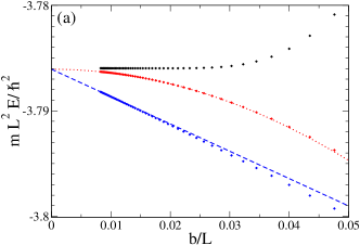
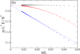
Figure 1: (Color online) Illustration of the Juillet effect for the lattice model: In the cubic box $[0,L]^{3}$ with periodic boundary conditions, ground state energy of two opposite spin fermions as a function of the grid spacing $b$, for an infinite scattering length ($1/a=0$), for a total momentum equal to $\mathbf{0}$ in (a) and equal to $\frac{2\pi\hbar}{L}\mathbf{e}_{z}$ in (b). Three dispersion relations $\epsilon_{\mathbf{k}}$ are considered, the quartic one of Eq. (120) with zero effective range $r_{e}=0$ (in blue, lower set), and the magic one (122) with $r_{e}=R_{e}=0$ with the parameters of Eq. (123) (in black, upper set) and of Eq. (124) (in red, middle set). The fact that the energy varies linearly in $b$ for the $r_{e}=0$ quartic dispersion relation at zero total momentum is the Juillet effect explained in Sec. VII.3, and the corresponding dashed line is the analytical result (134). At non-zero total momentum the quartic dispersion relation leads to an energy variation linear in $b$ as expected e.g. from the fact that its has a non-zero $R_{e}$ [the dotted line is a linear fit for $b/L\leq 0.01$]. The magic dispersion relations lead to a $O(b^{2})$ variation of the energy both at zero and non-zero total momentum [the dotted lines are purely quadratic fits performed for $b/L\leq 0.02$].

With the lattice dispersion relation $\epsilon_{\mathbf{k}}$ of (120), adjusted to have a zero effective range $r_{e}=0$, Olivier Juillet numerically observed, for two particles in the cubic box $[0,L]^{3}$ with periodic boundary conditions and zero total momentum, that the first energy correction to the zero-range limit $b\to 0$ is linear in $b$ Juillet , which seems to contradict [Tab. V, Eq. (1a)]. This is illustrated in Fig. 1. This cannot be explained by a non-zero $R_{e}$ [defined in Eq. (116)] because the two opposite-spin fermions have here a zero total momentum.

This Juillet effect, as we shall see, is due to the fact that the integral of $1/\epsilon_{\mathbf{k}}$ over $\mathbf{k}$ in the first Brillouin zone and the corresponding discrete sum for the finite size quantization box differ for $b/L\to 0$ not only by a constant term but also by a term linear in $b$, when the dispersion relation has a cusp at the surface of the first Brillouin zone, such as Eq. (120). The Juillet effect thus disappears in the thermodynamic limit. This explains why it does not show up in the diagrammatic point of view of Sec. VII.2, which was considered in the thermodynamic limit, so that only momentum integrals appeared. This also shows that the Juillet effect does not invalidate [Tab. V, Eq. (1a)] since it was derived for an interaction that is smooth in momentum space.

In Pricoupenko and Castin (2007b) it was shown that the lattice model spectrally reproduces the zero-range model when the grid spacing $b\to 0$. We now simply extend the reasoning of Pricoupenko and Castin (2007b) for two particles to first order in $b$ included. For an eigenenergy $E$ which does not belong to the non-interacting spectrum, the exact implicit equation is

$$\frac{1}{g_{0}}+\frac{1}{L^{3}}\sum_{\mathbf{k}\in D}\frac{1}{2\epsilon_{\mathbf{k}}-E}=0$$ (128)

where the notation with a discrete sum over $\mathbf{k}$ implicitly restricts $\mathbf{k}$ to $\frac{2\pi}{L}\mathbb{Z}^{3}$. By adding and subtracting terms, and using the expressions (11) and (115) for the bare coupling constant $g_{0}$ and the effective range $r_{e}$, one obtains the useful form:

$$\frac{1}{g}-\frac{m^{2}Er_{e}}{8\pi\hbar^{4}}+\frac{1}{L^{3}}\Bigg{[}-\frac{1}{E}+\!\!\sum_{\mathbf{k}\in D^{*}}F(\epsilon_{\mathbf{k}})+\!\!\sum_{\mathbf{k}\in{\mathbb{R}^{3}}^{*}}\frac{E}{(\hbar^{2}k^{2}/m)^{2}}\Bigg{]}\\ =R_{1}+ER_{2}-ER_{3}$$ (129)

with $g=4\pi\hbar^{2}a/m$ and $F(\epsilon)=(2\epsilon-E)^{-1}-(2\epsilon)^{-1}-E/(2\epsilon)^{2}$. We have defined

$$R_{1}\equiv\int_{D}\frac{d^{3}k}{(2\pi)^{3}}\frac{1}{2\epsilon_{\mathbf{k}}}-\frac{1}{L^{3}}\sum_{\mathbf{k}\in D^{*}}\frac{1}{2\epsilon_{\mathbf{k}}},$$ (130)

proportional to the function $C(b)$ introduced in Pricoupenko and Castin (2007b). The quantities $R_{2}$ and $R_{3}$ have the same structure: $R_{2}$ is obtained by replacing in $R_{1}$ the function $1/(2\epsilon_{\mathbf{k}})$ by $1/(2\epsilon_{\mathbf{k}})^{2}-1/(\hbar^{2}k^{2}/m)^{2}$, in the integral and in the sum; $R_{3}$ is obtained by replacing in $R_{1}$ the function $1/(2\epsilon_{\mathbf{k}})$ by $1/(\hbar^{2}k^{2}/m)^{2}$ and the set $D$ by $\mathbb{R}^{3}\setminus D$, both for the integration and for the summation.

We now take $b\to 0$ in Eq. (129), keeping terms up to $O(b)$ included. Since $F(\epsilon)=O(1/\epsilon^{3})$ at large $\epsilon$, we can replace $F(\epsilon_{\mathbf{k}})$ by its $b\to 0$ limit $F(\hbar^{2}k^{2}/2m)$, and the summation set $D^{*}$ by its $b\to 0$ limit :

$$\sum_{\mathbf{k}\in D^{*}}F(\epsilon_{\mathbf{k}})\underset{b\to 0}{=}\sum_{\mathbf{k}\in{\mathbb{R}^{3}}^{*}}F\left(\frac{\hbar^{2}k^{2}}{2m}\right)+O(b^{2})$$ (131)

In the quantities $R_{i}$, we perform the change of variables $\mathbf{k}=2\pi\mathbf{q}/b$, and we write the dispersion relation as

$$\epsilon_{\mathbf{k}}=\frac{(2\pi\hbar)^{2}}{mb^{2}}\eta_{\mathbf{k}b/(2\pi)}$$ (132)

where the dimensionless $\eta_{\mathbf{q}}$ does not depend on the lattice spacing $b$. We then find that $bR_{1}$, $R_{2}/b$ and $R_{3}/b$ are differences between a converging integral and a three-dimensional Riemann sum with a vanishing cell volume $(b/L)^{3}$. As these differences vanish as $O(b)$, we conclude that $R_{2}=O(b^{2})$ and $R_{3}=O(b^{2})$ can be neglected in Eq. (129). This however leads only to $R_{1}=O(1)$, so that more mathematical work needs to be done, as detailed in the Appendix F, to obtain

$$\frac{\hbar^{2}}{m}LR_{1}\underset{b\to 0}{=}\frac{\mathcal{C}}{4\pi^{2}}+\frac{\pi R_{e}^{\rm surf}}{2L}+O(b/L)^{2}.$$ (133)

The numerical constant $\mathcal{C}\simeq 8.91363$ was calculated and called $C(0)$ in Pricoupenko and Castin (2007b). $R_{e}^{\rm surf}$ remarkably is the surface contribution to the quantity $R_{e}$ in Eq. (116), it scales as $b$. It is non-zero only when the dispersion relation has a cusp at the surface of the first Brillouin zone. In this case, $R_{1}$ varies to first order in $b$, which comes in addition to the expected linear contribution of the $Er_{e}$ term in Eq. (129): This leads to the Juillet effect. More quantitatively, the first deviation of the eigenenergy from its zero-range limit $E^{0}$, shown as a dashed line in Fig. 1a, is :

$$E-E^{0}\underset{b\to 0}{\sim}\frac{\frac{m^{2}E^{0}r_{e}}{8\pi\hbar^{4}}+\frac{m\pi R_{e}^{\rm surf}}{2\hbar^{2}L^{2}}}{\frac{1}{L^{3}}\sum_{\mathbf{k}\in\mathbb{R}^{3}}\frac{1}{\left(\frac{\hbar^{2}k^{2}}{m}-E^{0}\right)^{2}}}$$ (134)

VII.4 Link between $\partial E/\partial r_{e}$ and the subleading short distance behavior of the pair distribution function

As shown by [Tab. II, Eqs. (3a,3b)] the short distance behavior of the pair distribution function (averaged over the center of mass position of the pair) diverges as $1/r^{2}$ in $3D$ and as $\ln^{2}r$ in $2D$, with a coefficient proportional to $C$, that is related to the derivative of the energy with respect to the scattering length $a$. Here we show that a subleading term in this short distance behavior is related to the derivative of the energy with respect to the effective range $r_{e}$. To this end, we explicitly write the next order term in the contact conditions [Tab. I, Eqs. (1a,1b)].

Three dimensions: Including the next order term in [Tab. I, Eq. (1a)] gives

$$\psi(\mathbf{r}_{1},\ldots,\mathbf{r}_{N})\underset{r_{ij}\to 0}{=}\left(\frac{1}{r_{ij}}-\frac{1}{a}\right)\,A_{ij}\left(\mathbf{R}_{ij},(\mathbf{r}_{k})_{k\neq i,j}\right)\\ +r_{ij}\ B_{ij}\left(\mathbf{R}_{ij},(\mathbf{r}_{k})_{k\neq i,j}\right)+\sum_{\alpha=1}^{3}r_{ij,\alpha}L_{ij}^{(\alpha)}\left(\mathbf{R}_{ij},(\mathbf{r}_{k})_{k\neq i,j}\right)\\ +O(r_{ij}^{2})$$ (135)

where we have distinguished between a singular part linear with the interparticle distance $r_{ij}$ and a regular part linear in the relative coordinates of $i$ and $j$ ($r_{ij,\alpha}$ is the component along axis $\alpha$ of the vector $\mathbf{r}_{ij}$). Injecting this form into Schrödinger’s equation, keeping the resulting $\propto 1/r_{ij}$ terms and using notation [Tab. V, Eq. (2)] gives

$$B_{ij}(\mathbf{R}_{ij},(\mathbf{r}_{k})_{k\neq i,j})=-\frac{m}{2\hbar^{2}}(E-\mathcal{H}_{ij})A_{ij}\left(\mathbf{R}_{ij},(\mathbf{r}_{k})_{k\neq i,j}\right)$$ (136)

[Tab. V, Eq. (1a)] thus becomes

$$\frac{\partial E}{\partial r_{e}}=-\frac{4\pi\hbar^{2}}{m}(A,B)$$ (137)

We square (135) and as in Sec. IV.2 we integrate over $\mathbf{R}_{ij}$, the $\mathbf{r}_{k}$’s and we sum over $i<j$. We further average $G^{(2)}_{\uparrow\downarrow}(\mathbf{r})$ over the direction of $\mathbf{r}$ to eliminate the contribution of the regular term $L_{ij}$, defining $\bar{G}^{(2)}_{\uparrow\downarrow}(\mathbf{r})=[G^{(2)}_{\uparrow\downarrow}(\mathbf{r})+G^{(2)}_{\uparrow\downarrow}(-\mathbf{r})]/2$. We obtain [Tab. V, Eq. (3a)].

Two dimensions: Including next order terms in [Tab. I, Eq. (1b)] gives :

$$\psi(\mathbf{r}_{1},\ldots,\mathbf{r}_{N})\underset{r_{ij}\to 0}{=}\ln(r_{ij}/a)\,A_{ij}\left(\mathbf{R}_{ij},(\mathbf{r}_{k})_{k\neq i,j}\right)\\ +r^{2}_{ij}\ln r_{ij}\ B_{ij}\left(\mathbf{R}_{ij},(\mathbf{r}_{k})_{k\neq i,j}\right)+\sum_{\alpha=1}^{2}r_{ij,\alpha}L_{ij}^{(\alpha)}\left(\mathbf{R}_{ij},(\mathbf{r}_{k})_{k\neq i,j}\right)\\ +O(r_{ij}^{2})$$ (138)

Proceeding as in $3D$ we obtain

$$B_{ij}(\mathbf{R}_{ij},(\mathbf{r}_{k})_{k\neq i,j})=-\frac{m}{4\hbar^{2}}(E-\mathcal{H}_{ij})A_{ij}\left(\mathbf{R}_{ij},(\mathbf{r}_{k})_{k\neq i,j}\right)$$ (139)

[Tab. V, Eq. (1b)] thus becomes

$$\frac{\partial E}{\partial(r_{e}^{2})}=-\frac{4\pi\hbar^{2}}{m}(A,B)$$ (140)

These equations finally leads to [Tab. V, Eq. (3b)].

VII.5 Link between $\partial E/\partial r_{e}$ and the $1/k^{6}$ subleading tail of the momentum distribution

A general idea given in Olshanii and Dunjko (2003) is that singular terms in the dependence of $\psi$ on the interparticle distance $r_{ij}$ (at short distances) reflect into power-law tails in the momentum distribution $n_{\sigma}(\mathbf{k})$ given by Eq. (23). In Sec. IV.1, we restricted to the leading order. Here we include the subleading term and we perform the same reasoning as in Sec. IV.1 to obtain

$$\bar{n}_{\sigma}(k)\underset{k\to\infty}{=}\frac{C}{k^{4}}+\frac{D}{k^{6}}+\ldots$$ (141)

where $\bar{n}_{\sigma}(k)=\frac{1}{d}\sum_{i=1}^{d}n_{\sigma}(k\mathbf{u}_{i})$ and $D$ is the linear combination of $\partial E/\partial r_{e}$ and $(A,\Delta_{\mathbf{R}}A)$ given in [Tab. V, Eqs. (4a,4b)]. Physically, the extra term $(A,\Delta_{\mathbf{R}}A)$ results from the fact that the wavevector $\mathbf{k}_{1}$ of a particle in an $\uparrow\downarrow$ colliding pair is a linear combination of the relative wavevector $\mathbf{k}_{\rm rel}$ and of the center-of-mass wavevector $\mathbf{K}$ of the pair, so that, even if the probability distribution of $\mathbf{k}_{\rm rel}$ was exactly scaling as $1/k_{\rm rel}^{4}$, a non-zero $\mathbf{K}$ would generate a subleading $1/k_{1}^{6}$ contribution in the single particle momentum distribution.

This is apparent for the simple case of a free space dimer: When the dimer is at rest, $\psi(\mathbf{r}_{1},\mathbf{r}_{2})=\phi_{\rm dim}(r_{12})$, $A_{12}(\mathbf{R}_{12})$ is uniform and the extra term vanishes. When it has a momentum $\mathbf{K}$, $\psi(\mathbf{r}_{1},\mathbf{r}_{2})=e^{i\mathbf{K}\cdot\mathbf{R}_{12}}\phi_{\rm dim}(r_{12})$, which shifts the single particle momentum distribution, $n_{\uparrow}^{\rm mov}(\mathbf{k})=n_{\uparrow}^{\rm rest}(\mathbf{k}-\mathbf{K}/2)$. Applying this shift to the momentum tail $C/k^{4}$ gives, after continuous average over the direction of $\mathbf{k}$, a subleading $\delta D^{\rm mov}/k^{6}$ contribution, with $\delta D^{\rm mov}=CK^{2}/2$ in $3D$ and $\delta D^{\rm mov}=CK^{2}$ in $2D$. Remarkably, the ratio of the extra term to $C$ is proportional to the pair-center-of-mass kinetic energy.

In the $N$-body case, one can generalize this property by defining the mean center-of-mass kinetic energy of a $\uparrow\downarrow$ pair at vanishing pair diameter, which is allowed in quantum mechanics since the center-of-mass operators and the relative-particle operators commute . By a direct generalisation of the pair distribution function of Sec. IV.2, one has for the opposite-spin pair density operator $\langle\mathbf{r}_{\uparrow},\mathbf{r}_{\downarrow}|\hat{\rho}_{\uparrow\downarrow}^{(2)}|\mathbf{r}_{\uparrow}^{\prime},\mathbf{r}_{\downarrow}^{\prime}\rangle=\langle\hat{\psi}_{\uparrow}^{\dagger}(\mathbf{r}_{\uparrow}^{\prime})\hat{\psi}^{\dagger}_{\downarrow}(\mathbf{r}_{\downarrow}^{\prime})\hat{\psi}_{\downarrow}(\mathbf{r}_{\downarrow})\hat{\psi}_{\uparrow}(\mathbf{r}_{\uparrow})\rangle$. Whereas the usual pair-center-of-mass density operator is obtained by taking the trace over the relative coordinates $\mathbf{r}=\mathbf{r}_{\uparrow}-\mathbf{r}_{\downarrow}$, we rather define it here by taking the limit of vanishing relative coordinates,

$$\langle\mathbf{R}|\hat{\rho}_{\rm CoM}^{(2)}|\mathbf{R}^{\prime}\rangle=\mathcal{N}\lim_{r\to 0}\frac{\langle\mathbf{R}+\frac{\mathbf{r}}{2},\mathbf{R}-\frac{\mathbf{r}}{2}|\hat{\rho}_{\uparrow\downarrow}^{(2)}|\mathbf{R}^{\prime}+\frac{\mathbf{r}}{2},\mathbf{R}^{\prime}-\frac{\mathbf{r}}{2}\rangle}{\phi^{2}(\mathbf{r})}$$ (142)

where the factor $\mathcal{N}$ is such that $\hat{\rho}_{\rm CoM}^{(2)}$ has a unit trace and $\phi(\mathbf{r})$ is the zero-energy scattering state of Eqs.(9,10). Proceeding as in Sec. IV.2 we obtain

$$\langle\mathbf{R}|\hat{\rho}_{\rm CoM}^{(2)}|\mathbf{R}^{\prime}\rangle=\mathcal{N}\sum_{i<j}\int(\prod_{k\neq i,j}d^{d}r_{k})A_{ij}^{*}(\mathbf{R}^{\prime},(\mathbf{r}_{k})_{k\neq i,j})\\ \times A_{ij}(\mathbf{R},(\mathbf{r}_{k})_{k\neq i,j})$$ (143)

By taking the expectation value of $-(\hbar^{2}/4m)\Delta_{\mathbf{R}}$ within $\hat{\rho}_{\rm CoM}^{(2)}$, we finally obtain for the mean pair-center-of-mass kinetic energy at vanishing diameter:

$$E_{\rm kin\ pair-CoM}^{r_{\uparrow\downarrow}\to 0}=-\frac{\hbar^{2}}{4m}\frac{(A,\Delta_{\mathbf{R}}A)}{(A,A)}$$ (144)

where the denominator is $\propto C$, see [Tab. II, Eqs. (2a,2b)].

VIII Generalization to arbitrary statistical mixtures

In this section, we generalize some of the relations derived in the previous sections for pure states to the case of arbitrary statistical mixtures. Let us first discuss zero-range interactions. We consider a statistical mixture of pure states $\psi_{n}$ with occupation probabilities $p_{n}$, which is arbitrary, but non-pathological in the following sense Tan (2008a): Each $\psi_{n}$ satisfies the contact condition [Tab. I, Eqs. (1a,1b)]; moreover, $p_{n}$ decays sufficiently quickly at large $n$ so that we have $\displaystyle C=\sum_{n}p_{n}C_{n}$, where $C_{n}$ (resp. $C$) is defined by [Tab. II, Eq. (1)] with $n_{\sigma}(\mathbf{k})=\langle c^{\dagger}_{\sigma}(\mathbf{k})c_{\sigma}(\mathbf{k})\rangle$ and $\langle\,.\,\rangle=\langle\psi_{n}|\,.\,|\psi_{n}\rangle$ (resp. $\langle\,.\,\rangle=\sum_{n}p_{n}\langle\psi_{n}|\,.\,|\psi_{n}\rangle$). Then, the relations in lines 3, 5, 6 and 7 of Table II, which were derived in Sec. IV for any pure state satisfying the contact conditions, obviously generalize to such a statistical mixture. The relations for the time derivative of $E$ (Tab. 2 line 12) hold for any time-evolving pure state satisfying the contact conditions for a time-dependent $a(t)$, and thus also for any statistical mixture of such time-evolving pure states.

For lattice models, one can obviously take an average of the definition of $\hat{C}$ [Tab. III, Eqs. (1a,1b)] to define $C=\langle\hat{C}\rangle$ for in any statistical mixture; taking averages of the relations between operators [Tab.III, lines 2,3,8] then gives relations valid for any statistical mixture.

IX Thermodynamic equilibrium in the canonical ensemble

We turn to the case of thermal equilibrium in the canonical ensemble. We shall use the notation

$$\lambda\equiv\left\{\begin{array}[]{lr}-1/a&{\rm in}\ 3D\\ \frac{1}{2}\ln a&{\rm in}\ 2D.\end{array}\right.$$ (145)

IX.1 First order derivative of $E$

The thermal average in the canonical ensemble $\overline{dE/d\lambda}$ can be rewritten in the following more familiar way, as detailed in Appendix G:

$$\overline{\left(\frac{dE}{d\lambda}\right)}=\left(\frac{dF}{d\lambda}\right)_{\!T}=\left(\frac{d\bar{E}}{d\lambda}\right)_{\!S}$$ (146)

where $\overline{(\dots)}$ is the canonical thermal average, $F$ is the free energy and $S$ is the entropy. Taking the thermal average of [Tab. 2, Eqs. (4a,4b)] (which was shown above for any stationary state) thus gives [Tab. 2, Eqs. (9a,9b)].

IX.2 Second order derivative of $E$

Taking a thermal average of the line 8 in Tab. 2 we get after a simple manipulation:

$$\frac{1}{2}\overline{\left(\frac{d^{2}E}{d\lambda^{2}}\right)}=\left(\frac{4\pi\hbar^{2}}{m}\right)^{2}\frac{1}{2Z}\sum_{n,n^{\prime};E_{n}\neq E_{n^{\prime}}}\frac{e^{-\beta E_{n}}-e^{-\beta E_{n^{\prime}}}}{E_{n}-E_{n^{\prime}}}\\ \times|(A^{(n^{\prime})},A^{(n)})|^{2}$$ (147)

where $Z=\sum_{n}\exp(-\beta E_{n})$. This implies

$$\overline{\left(\frac{d^{2}E}{d\lambda^{2}}\right)}<0.$$ (148)

Moreover one can check that

$$\left(\frac{d^{2}F}{d\lambda^{2}}\right)_{T}-\overline{\left(\frac{d^{2}E}{d\lambda^{2}}\right)}=-\beta\left[\,\overline{\left(\frac{dE}{d\lambda}\right)^{\phantom{,}2}}-\overline{\left(\frac{dE}{d\lambda}\right)}^{\phantom{,}2}\right]<0,$$ (149)

which implies [Tab. II, Eqs. (10a,10b)]. In usual cold atom experiments, however, there is no thermal reservoir imposing a fixed temperature to the gas, one rather can achieve adiabatic transformations by a slow variation of the scattering length of the gas Cubizolles et al. (2003); Strecker et al. (2003); Bartenstein et al. (2004) where the entropy is fixed Landau and Lifchitz (1994); Carr et al. (2004); Werner et al. (2005). One also more directly accesses the mean energy $\bar{E}$ of the gas rather than its free energy, even if the entropy is also measurable Luo et al. (2007); Luo and Thomas (2009). The second order derivative of $\bar{E}$ with respect to $\lambda$ for a fixed entropy is thus the relevant quantity to consider. As shown in Appendix G one has in the canonical ensemble:

$$\left(\frac{d^{2}\bar{E}}{d\lambda^{2}}\right)_{S}=\overline{\left(\frac{d^{2}E}{d\lambda^{2}}\right)}+\frac{\left[\mbox{Cov}\!\left(E,\frac{dE}{d\lambda}\right)\right]^{2}-\mbox{Var}(E)\mbox{Var}\!\left(\frac{dE}{d\lambda}\right)}{k_{B}T\,\mbox{Var}(E)}$$ (150)

where $\mbox{Var}(X)$ and $\mbox{Cov}(X,Y)$ stand for the variance of the quantity $X$ and the covariance of the quantities $X$ and $Y$ in the canonical ensemble, respectively. From the Cauchy-Schwarz inequality $[\mbox{Cov}(X,Y)]^{2}\leq\mbox{Var}(X)\mbox{Var}(Y)$, and from the inequality (148), we thus obtain [Tab. II, Eqs. (11a,11b)].

For lattice models, the inequalities [Tab. III, Eq. (7)] are derived in the same way, by taking $\lambda$ now equal to $g_{0}$, and starting from the expression [Tab. III, Eq. (6)] of $d^{2}E_{n}/dg_{0}^{2}$. For the case of a finite-range interaction potential $V(r)$ in continuous space, the relations [Tab. IV, lines 1-3] which were derived for an arbitrary stationary state are generalized to the thermal equilibrium case in the same way. Finally, the relations which asymptotically hold in the zero-range regime, [Tab. III lines 9-10] for lattice models and [Tab. IV lines 4-5] for finite-range interaction potential models, which were justified for any eigenstate in the zero-range regime $k_{\rm typ}b<<1$ where the typical relative wavevector $k_{\rm typ}$ is defined in terms of the considered eigenstate as described in Section III, remain true at thermal equilibrium with $k_{\rm typ}$ now defined as the typical density- and temperature-dependent wavevector described in Section III, since all the eigenstates which are thermally populated with a non-negligible weight are expected to have a typical wavevector smaller or on the order of the thermal-equilibrium typical wavevector.

IX.3 Quantum-mechanical adiabaticity

To be complete, we also consider the process where $\lambda$ is varied so slowly that there is adiabaticity in the many-body quantum mechanical sense: The adiabatic theorem of quantum mechanics Kato (1950) implies that in the limit where $\lambda$ is changed infinitely slowly, the occupation probabilities of each eigenspace of the many-body Hamiltonian do not change with time, even in presence of level crossings Avron and Elgart (1999). We note that this may require macroscopically long evolution times for a large system. For an initial equilibrium state in the canonical ensemble, the mean energy then varies with $\lambda$ as

$$E^{\rm quant}_{\rm adiab}(\lambda)=\sum_{n}\frac{e^{-\beta_{0}E_{n}(\lambda_{0})}}{Z_{0}}\,E_{n}(\lambda)$$ (151)

where the subscript $0$ refers to the initial state. Taking the second order derivative of (151) with respect to $\lambda$ in $\lambda=\lambda_{0}$ gives

$$\frac{d^{2}E_{\rm adiab}^{\rm quant}}{d\lambda^{2}}=\overline{\left(\frac{d^{2}E}{d\lambda^{2}}\right)}<0.$$ (152)

Note that the sign of the second order derivative of $E_{\rm adiab}^{\rm quant}$ remains negative at all $\lambda$ provided one assumes that there is no level crossing in the many-body spectrum when $\lambda$ is varied: $E_{n}(\lambda)-E_{n^{\prime}}(\lambda)$ has the same sign as $E_{n}(\lambda_{0})-E_{n^{\prime}}(\lambda_{0})$ for all indices $n,n^{\prime}$, which allows to conclude on the sign with the same manipulation as the one having led to Eq. (147).

Thermodynamic vs quantum adiabaticity: The result of the isentropic transformation (150) and the one of the adiabatic transformation in the quantum sense (152) differ by the second term in the right hand side of (150). A priori this term is extensive, and thus not negligible as compared to the first term. We have explicitly checked this expectation for the Bogoliubov model Hamiltonian of a weakly interacting Bose gas, which is however not really relevant since this Bogoliubov model corresponds to the peculiar case of an integrable dynamics.

For a quantum ergodic system we now show that the second term in the right hand side of (150) is negligible in the thermodynamic limit, as a consequence of the Eigenstate Thermalization Hypothesis Deutsch (1991); Srednicki (1994, 1996, 1999). This Hypothesis was tested numerically for several interacting quantum systems Rigol et al. (2008); Rigol (2009a, b). It states that, for a large system, the expectation value $\langle\psi_{n}|\hat{O}|\psi_{n}\rangle$ of a few-body observable $\hat{O}$ in a single eigenstate $|\psi_{n}\rangle$ of energy $E_{n}$ can be identified with the microcanonical average $O_{\rm mc}(E_{n})$ of $\hat{O}$ at that energy. Here the relevant operator $\hat{O}$ is the two-body observable (the so-called contact operator) such that $\frac{d}{d\lambda}E_{n}=\langle\psi_{n}|\hat{O}|\psi_{n}\rangle$. In the canonical ensemble, the energy fluctuations scale as $\mathcal{V}^{1/2}$ where $\mathcal{V}$ is the system volume. We can thus expand the microcanonical average around the mean energy $\bar{E}$:

$$O_{\rm mc}(E)=O_{\rm mc}(\bar{E})+(E-\bar{E})O^{\prime}_{\rm mc}(\bar{E})+O(1)$$ (153)

To leading order, we then find that $\mbox{Cov}\!\left(E,\frac{dE}{d\lambda}\right)\sim O_{\rm mc}^{\prime}(\bar{E})\mbox{Var}\,E$ and $\mbox{Var}\!\left(\frac{dE}{d\lambda}\right)\sim[O_{\rm mc}^{\prime}(\bar{E})]^{2}\mbox{Var}\,E$, so that the second term in the right hand side of  (150) is $O(\mathcal{V}^{1/2})$ which is negligible as compared to the first term in that right hand side. For the considered quantity, this shows the equivalence of the thermodynamic adiabaticity and of the quantum adiabaticity for a large system.

A microcanonical detour: We now argue that the quantum adiabatic expression (151) for the mean energy as a function of the slowly varying parameter $\lambda$ can be obtained by a purely thermodynamic reasoning. This implies that the exponentially long evolution times a priori required to reach the quantum adiabatic regime for a large system are actually not necessary to obtain (151). The first step is to realize that the initial canonical ensemble (for $\lambda=\lambda_{0}$) can be viewed as a statistical mixture of microcanonical ensembles Sinatra et al. (2009). These microcanonical ensembles correspond to non-overlapping energy intervals of width $\Delta$, each interval contains many eigenstates, but $\Delta$ is much smaller than the width of the probability distribution of the system energy in the canonical ensemble. For further convenience, we take $\Delta\ll k_{B}T$. One can label each energy interval by its central energy value, or more conveniently by its entropy $S$. If the eigenenergies $E_{n}(\lambda)$ are numbered in ascending order, the initial microcanonical ensemble of entropy $S$ contains the eigenenergies with $n_{1}(S)\leq n<n_{2}(S)$ and $S=k_{B}\ln[n_{2}(S)-n_{1}(S)]$. When $\lambda$ is slowly varied, the entropy is conserved for our isolated system, and the microcanonical ensemble simply follows the evolution of the initial $n_{2}(S)-n_{1}(S)$ eigenstates, which cannot cross for an ergodic system and remain bunched in energy space. Furthermore, according to the Eigenstate Thermalization Hypothesis, the energy width $E_{n_{2}}-E_{n_{1}}$ remains close to its initial value $\Delta$: Each eigenenergy varies with a macroscopically large slope $dE_{n}/d\lambda$ but all the eigenenergies in the microcanonical ensemble have essentially the same slope . The mean microcanonical energy for this isentropic evolution is thus

$$E_{\rm mc}(S,\lambda)=\frac{1}{n_{2}(S)-n_{1}(S)}\sum_{n=n_{1}(S)}^{n_{2}(S)-1}E_{n}(\lambda)$$ (154)

Finally, we take the appropriate statistical mixture of the microcanonical ensembles (so as to reconstruct the initial $\lambda=\lambda_{0}$ canonical ensemble): The microcanonical ensemble of entropy $S$ has an initial central energy $E_{\rm mc}(S,\lambda_{0})$, it is weighted in the statistical mixture by the usual expression $P(S)=e^{S/k_{B}}e^{-\beta E_{\rm mc}(S,\lambda_{0})}$. Since $\Delta\ll k_{B}T$, one can identify $e^{-\beta E_{\rm mc}(S,\lambda_{0})}$ with $e^{-\beta E_{n}(\lambda_{0})}$, for $n_{1}(S)\leq n<n_{2}(S)$. The corresponding statistical average of (154) with the weight $P(S)$ gives (151).

X Applications

In this Section, we apply some of the above relations in three dimensions, first to the two-body and three-body problems and then to the many-body problem. Except for the two-body case, we restrict to the infinite scattering length case $a=\infty$ in three dimensions.

X.1 Two-body problem in a harmonic trap: Finite range corrections

Two particles interact with the compact-support potential $V(r_{12};b)$ of range $b$ and scattering length $a$ in an isotropic harmonic potential $U(\mathbf{r}_{i})=\frac{1}{2}m\omega^{2}r_{i}^{2}$. One separates out the center of mass, in an eigenstate of energy $E_{\rm cm}$. The relative motion is taken with zero angular momentum; its wavefunction $\psi(r)$ is an eigenstate of energy $E_{\rm rel}=E-E_{\rm cm}$ for a particle of mass $\mu=m/2$ in the potential $V(r;b)+\mu\omega^{2}r^{2}/2$. We take in this subsection $\hbar\omega$ as the unit of energy and $[\hbar/(\mu\omega)]^{1/2}$ as the unit of length. For $r\geq b$ the solution may be expressed in terms of the Whittaker function $W$, or equivalently of the Kummer function $U$, see §13 in Abramowitz and Stegun (1970):

$$\frac{\psi(r)}{C_{3}}\!\!\! \stackrel{{\scriptstyle 3D}}{{=}} \!\!\!\frac{W_{\frac{E_{\rm rel}}{2},\frac{1}{4}}(r^{2})}{r^{3/2}}=e^{-\frac{r^{2}}{2}}U(\frac{3}{4}-\frac{E_{\rm rel}}{2},\frac{3}{2},r^{2})$$ (155)

$$\frac{\psi(r)}{C_{2}}\!\!\! \stackrel{{\scriptstyle 2D}}{{=}} \!\!\!\frac{W_{\frac{E_{\rm rel}}{2},0}(r^{2})}{r}=e^{-\frac{r^{2}}{2}}U(\frac{1-E_{\rm rel}}{2},1,r^{2})$$ (156)

where the factors $C_{2}$ and $C_{3}$ ensure that $\psi$ is normalized to unity. The zero-range limit, where $V(r;b)$ is replaced by the Bethe-Peierls contact conditions at the origin, is exactly solvable; it gives eigenenergies $E_{\rm rel}^{0}$. We give here the finite range corrections to the energy in terms of $r_{e}$.

Three dimensions:
Imposing the contact condition $\psi(r)=A[r^{-1}-a^{-1}]+O(r)$ to Eq. (155) gives an implicit equation for the spectrum in the zero-range limit, obtained in Busch et al. (1998) with a different technique:

$$f(E_{\rm rel}^{0})=-\frac{1}{a}\ \ \ \mbox{with}\ \ \ f(E)\equiv-\frac{2\Gamma(\frac{3}{4}-\frac{E}{2})}{\Gamma(\frac{1}{4}-\frac{E}{2})}$$ (157)

We have calculated the finite range corrections up to order two in $b$ included, they remarkably involve only the effective range:

$$E_{\rm rel}=E_{\rm rel}^{0}+\frac{E_{\rm rel}^{0}r_{e}}{f^{\prime}}+\left(\frac{E_{\rm rel}^{0}r_{e}}{f^{\prime}}\right)^{2}\left(\frac{1}{E_{\rm rel}^{0}}-\frac{f^{\prime\prime}}{2f^{\prime}}\right)+O(b^{3})$$ (158)

where the first and second order derivatives $f^{\prime}$ and $f^{\prime\prime}$ of $f(E)$ are taken in $E=E_{\rm rel}^{0}$. To obtain this expansion, we have used the result of Appendix D that one can neglect, at this order, the effect of the trapping potential for $r\leq b$, so that the wavefunction is proportional to the free space scattering state at energy $E_{\rm rel}=\hbar^{2}k^{2}/(2\mu)$, $\psi(r)=\mathcal{A}\chi(r)$. Such an approximation was already proposed in Bolda et al. (2002); Naidon et al. (2007); Chen and Gao (2007), without analytical control on the resulting spectral error . We have checked that the term of Eq. (158) linear in $r_{e}$ coincides with the prediction of [Tab. V, Eq. (1a)], due to the fact that, from relation 7.611(4) in Gradshteyn and Ryzhik (1994), the normalization factor in the zero-range limit obeys $(C_{3}^{0})^{2}2\pi^{2}f^{\prime}(E_{\rm rel}^{0})/\Gamma^{2}(\frac{3}{4}-\frac{E_{\rm rel}^{0}}{2})=1$.

The term in Eq. (158) linear in $r_{e}$ was already written explicitly in Werner (2008a). This corresponds to the first order perturbative use of the modified version of the zero-range model, as put forward in Efimov (1993). It can also be obtained by solving to first order in $r_{e}$ the self-consistent equation considered in Blume and Greene (2002) obtained by replacing $a_{0}$ by $a_{E}$ [see Eq. (5) of Blume and Greene (2002)] into Eq. (6) of Blume and Greene (2002). This self-consistent equation was also introduced in Bolda et al. (2002), and in Chen and Gao (2007) [see Eqs. (11,12,30) of that reference] with more elaborate forms for $a_{E}$. With our notations and units this self-consistent equation is simply

$$f(E)=-u(k=\sqrt{2E})$$ (159)

where $u(k)$ is related to the $s$-wave scattering amplitude by Eq. (90). The self-consistent equation of Blume and Greene (2002) corresponds to the choice $u(k)=\frac{1}{a}-\frac{1}{2}k^{2}r_{e}$ in Eq. (159). We have checked that solving that equation to second order in $r_{e}$ then exactly gives the term of Eq. (158) that is quadratic in $r_{e}$. Our result of Appendix D shows that going to order three in $r_{e}$ with the self-consistent equation should not give the correct result, since one can then no longer neglect the effect of harmonic trapping within the interaction range. This clarifies the status of that self-consistent equation.

To ascertain this statement, we have calculated the ground state relative energy up to third order included in $b$, restricting for simplicity to an infinite scattering length, $1/a=0$ . We find

$$E_{\rm rel}=\frac{1}{2}+\frac{r_{e}}{2\pi^{1/2}}+\frac{2-\ln 2}{4\pi}r_{e}^{2}+\Big{[}\frac{(1-\ln 2)(2-\ln 2)}{4\pi^{3/2}}\\ -\frac{\pi^{2}+12\ln^{2}2}{192\pi^{3/2}}\Big{]}r_{e}^{3}-\frac{\lambda_{2}+\Lambda_{2}}{\pi^{1/2}}+O(b^{4})$$ (160)

Here $\lambda_{2}$ is the coefficient of $k^{4}$ in the low-$k$ expansion of $u(k)$, $u(k)=\frac{1}{a}-\frac{1}{2}k^{2}r_{e}+\lambda_{2}k^{4}+O(k^{6})$, it can be evaluated by a generalized Smorodinski relation Castin (a). On the contrary, $\Lambda_{2}$ is a new coefficient containing the effect of the trapping potential within the interaction range. It can be expressed in terms of the zero-energy free space scattering state $\phi(r)$, normalized as in Eq. (9):

$$\Lambda_{2}=\int_{0}^{+\infty}dr\,r^{2}[1-u_{0}^{2}(r)]$$ (161)

with $u_{0}(r)=r\phi(r)$. Although our derivation is for a compact support potential, we expect that our result is applicable as long as $\lambda_{2}$ and $\Lambda_{2}$ are finite. For both quantities, this requires (for $1/a=0$) that the interaction potential drops faster than $1/r^{5}$ Castin (a). Interestingly, if one expands the self-consistent Eq. (159) up to order $b^{3}$ included, one exactly recovers Eq. (160), except for the term $\Lambda_{2}$. This was expected from the fact that the derivation of (159) in Chen and Gao (2007) indeed neglects the trapping potential within the interaction range.

This discussion is illustrated for the particular case of the square-well potential (182) in Fig.2, with the exact spectrum obtained by matching the logarithmic derivative of a Whittaker $M$ function for $r=b^{-}$ with the logarithmic derivative of a Whittaker $W$ function for $r=b^{+}$ as in Eqs. (6.16,6.17,6.18) of Werner (2008a) . In this case, one finds $r_{e}=b$ Castin (2007) and, remarkably, $\Lambda_{2}=-2\lambda_{2}$ so that the difference between the ground state energy of (159) and the exact ground state energy obeys

$$E_{\rm rel}^{\rm self}-E_{\rm rel}=\frac{\Lambda_{2}}{\pi^{1/2}}+O(b^{4})=\left(\frac{1}{6}-\frac{1}{\pi^{2}}\right)\frac{b^{3}}{\pi^{1/2}}+O(b^{4}).$$ (162)

Note that the case of two fermions with a square-well interaction in a harmonic trap was numerically studied in Idziaszek and Calarco (2006), for the $s$-wave and also for the $p$-wave case, with the exact spectrum compared to the self-consistent equation (159) or to its $p$-wave equivalent. No conclusion was given on the scaling with $b$ of the difference between the exact and the approximate spectrum.

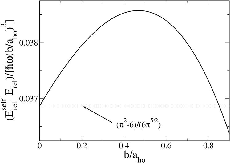
Figure 2: For two opposite spin fermions interacting in $3D$ via a potential of short range $b$ in an isotropic harmonic trap, the self-consistent equation (159), derived e.g. in Chen and Gao (2007), gives the eigenenergies with an error of order $b^{3}$, due to the fact that it neglects the effect of the harmonic trap within the interaction range, see Appendix D. This is illustrated with the ground state relative energy for a square-well potential of infinite scattering length: The deviation (solid line) between the approximate energy $E_{\rm rel}^{\rm self}$ [solving Eq. (159)] and the exact one $E_{\rm rel}$ (calculated as in Werner (2008a)) vanishes as $b^{3}$, with a coefficient given by Eq. (162) (dotted line). $\mu$ is the reduced mass, $\omega$ is the angular oscillation frequency in the trap and $a_{\rm ho}=[\hbar/(\mu\omega)]^{1/2}$.

Two dimensions:
Imposing the contact condition $\psi(r)=A\ln(r/a)+O(r)$ to Eq. (156) gives an implicit equation for the spectrum in the zero-range limit Busch et al. (1998); Castin and Werner :

$$\psi\left(\frac{1-E_{\rm rel}^{0}}{2}\right)-2\psi(1)=-2\ln a$$ (163)

where $\psi$ is the digamma function. We have obtained the finite range correction

$$E_{\rm rel}=E_{\rm rel}^{0}+\frac{4r_{e}^{2}E_{\rm rel}^{0}}{\psi^{\prime}(\frac{1-E_{\rm rel}^{0}}{2})}+O(b^{4}\ln^{4}b)$$ (164)

by neglecting the trapping potential for $r\leq b$ as justified by Appendix D, and by matching in $r=b$ the scattering state $\mathcal{A}\chi(r)$ to Eq. (156). The bound on the error results in particular from the statement that $\ldots$ in Eq. (97) are $O[(kb)^{4}\ln(a/b)]$, that one can e.g. check for the square-well potential. As expected, the value of $\partial E_{\rm rel}/\partial(r_{e}^{2})$ in $r_{e}=0$ obtained from Eq. (164) coincides with [Tab, V, Eq. (1b)], knowing that the normalization factor in the zero-range limit, according to relation 7.611(5) in Gradshteyn and Ryzhik (1994), obeys $(C_{2}^{0})^{2}\pi\psi^{\prime}(\frac{1-E_{\rm rel}^{0}}{2})/\Gamma^{2}(\frac{1-E_{\rm rel}^{0}}{2})=1$.

X.2 Three-body problem: corrections to exactly solvable cases and comparison with numerics

In this Subsection, we use the known analytical expressions for the three-body wavefunctions to compute the corrections to the spectrum to first order in the inverse scattering length $1/a$ and in the effective range $r_{e}$. We shall consider not only spin-1/2 fermions, but also spinless bosons restricting to the universal stationary states Werner and Castin (2006a); Jonsell et al. (2002) which do not depend on the three-body parameter.

The problem of three identical spinless bosons Werner and Castin (2006a); Jonsell et al. (2002) or spin-1/2 fermions (say $N_{\uparrow}=2$ and $N_{\downarrow}=1$) Werner and Castin (2006a); Tan (b) is exactly solvable in the unitary limit in an isotropic harmonic trap $U(\mathbf{r})=\frac{1}{2}\,m\omega^{2}r^{2}$. Here we restrict to zero total angular momentum (see however the last line of Appendix H) with a center of mass in its ground state, so that the normalization constants of the wavefunctions are also known analytically Werner (2008a). Moreover we restrict to universal eigenstates . The spectrum is then

$$E=E_{\rm cm}+(s+1+2q)\hbar\omega$$ (165)

where $E_{\rm cm}$ is the energy of the center of mass motion, $s$ belongs to the infinite set of real positive solutions of

$$-s\cos\left(s\frac{\pi}{2}\right)+\eta\frac{4}{\sqrt{3}}\sin\left(s\frac{\pi}{6}\right)=0$$ (166)

with $\eta=+2$ for bosons and $-1$ for fermions, and $q$ is a non-negative integer quantum number describing the degree of excitation of an exactly decoupled bosonic breathing mode Castin (2004); Werner and Castin (2006b). We restrict to states with $q=0$. The case of a non-zero $q$ is treated in subsection X.3.

Derivative of the energy with respect to $1/a$.

Injecting the expression of the regular part $A$ of the normalized wavefunction Werner (2008a) into [Tab. II, Eqs. (2a,4a)] or its bosonic version (Tab. V, line 1 in Werner and Castin (b)) we obtain

$$\frac{\partial E}{\partial(-1/a)}\Big{|}_{a=\infty}\!\!\!\!=\frac{\sqrt{\frac{\hbar^{3}\omega}{m}}\Gamma(s+\frac{1}{2})\sqrt{2}s\sin\left(s\frac{\pi}{2}\right)/\Gamma(s+1)}{-\cos\left(s\frac{\pi}{2}\right)+s\frac{\pi}{2}\sin\left(s\frac{\pi}{2}\right)+\eta\frac{2\pi}{3\sqrt{3}}\cos\left(s\frac{\pi}{6}\right)}$$ (167)

For the lowest fermionic state, this gives $(\partial E/\partial(1/a))_{a=\infty}\simeq-1.1980\sqrt{\hbar^{3}\omega/m}$, in agreement with the value $-1.19(2)$ which we extracted from the numerical solution of a finite-range model presented in Fig. 4a of von Stecher et al. (2008), where the error bar comes from our simple way of extracting the derivative from the numerical data of von Stecher et al. (2008).

Derivative of the energy with respect to the effective range.

Using relation [Tab. V, Eq. (1a)], which holds not only for fermions but also for bosonic universal states, we obtain

$$\left(\frac{\partial E}{\partial r_{e}}\right)_{a=\infty}\!\!\!\!\!=\frac{\sqrt{\frac{\hbar m\omega^{3}}{8}}\Gamma(s-\frac{1}{2})s(s^{2}-\frac{1}{2})\sin(s\frac{\pi}{2})/\Gamma(s+1)}{-\cos(s\frac{\pi}{2})+s\frac{\pi}{2}\sin(s\frac{\pi}{2})+\eta\,\frac{2\pi}{3\sqrt{3}}\cos(s\frac{\pi}{6})}$$ (168)

For bosons, this result was derived previously using the method of Efimov (1993) and found to agree with the numerical solution of a finite-range separable potential model for the lowest state Werner (2008a). For fermions, (168) agrees with the numerical data from Fig. 3 of von Stecher et al. (2008) to $\sim 0.3\%$ for the two lowest states and $5\%$ for the third lowest state ; (168) also agrees to $3\%$ with the numerical data from p. 21 of Werner (2008a) for the lowest state of a finite-range separable potential model. All these deviations are compatible with the estimated numerical accuracy.

X.3 $N$-body problem in an isotropic trap: Non-zero $1/a$ and $r_{e}$ corrections

We now generalize subsection X.2 to the case of an arbitrary number $N$ of spin-1/2 fermions (with an arbitrary spin configuration) at the unitary limit in an isotropic harmonic trap. Although one cannot calculate $\partial E/\partial(1/a)$ and $\partial E/\partial r_{e}$, some useful information can be obtained from the following remarkable property: For any initial stationary state, and after an arbitrary change of the isotropic trap curvature, the system experiences an undamped breathing at frequency $2\omega$, $\omega$ being the single atom oscillation frequency in the final trapping potential Castin (2004). From this one can conclude that, in the case of a time independent trap, the system exhibits a $SO(2,1)$ dynamical symmetry Werner and Castin (2006b): The spectrum is a collection of semi-infinite ladders indexed by the natural integer $q$. Another crucial consequence is that the eigenstate wavefunctions are separable in $N$-body hyperspherical coordinates, with a know expression for the dependence with the hyperradius Werner and Castin (2006b). This implies that the functions $A_{ij}$ are also separable in $(N-1)$-body hyperspherical coordinates and that their hyperradial dependence is also known. As the eigenstates within a ladder have exactly the same hyperangular part, one can relate the energy derivatives (with respect to $1/a$ or $r_{e}$) for step $q$ of a ladder to the derivative for the ground step of the same ladder, as detailed in Appendix H:

$$\left[\frac{\partial E}{\partial(1/a)}\right]_{q}=\left[\frac{\partial E}{\partial(1/a)}\right]_{0}\frac{\Gamma(s+1)}{\Gamma(s+q+1)}\\ \times\sum_{k=0}^{q}\left[\frac{\Gamma(k+\frac{1}{2})}{\Gamma(k+1)\Gamma(\frac{1}{2})}\right]^{2}\frac{\Gamma(s+q-k+\frac{1}{2})\Gamma(q+1)}{\Gamma(s+\frac{1}{2})\Gamma(q-k+1)}$$ (169)

with the eigenenergy of step $q$ is written as Eq. (165), $s$ being now unknown for the general $N$-body problem. We have checked that this explicit result is consistent with the recursion relations derived in Moroz (2012). A similar type of result holds for the derivative with respect to $r_{e}$:

$$\left[\frac{\partial E}{\partial r_{e}}\right]_{q}=\left[\frac{\partial E}{\partial r_{e}}\right]_{0}\frac{\Gamma(s+1)}{\Gamma(s+q+1)}\\ \times\sum_{k=0}^{q}\left[\frac{\Gamma(k+\frac{3}{2})}{\Gamma(k+1)\Gamma(\frac{3}{2})}\right]^{2}\frac{\Gamma(s+q-k-\frac{1}{2})\Gamma(q+1)}{\Gamma(s-\frac{1}{2})\Gamma(q-k+1)}$$ (170)

For non-zero $1/a$ or $r_{e}$, the level spacing is not constant within a ladder, the system will not respond to a trap change by a monochromatic breathing mode. In a small system, a Fourier transform of the system response can give access to the Bohr frequencies $(E_{q}-E_{q-1})/\hbar$, which would allow an experimental test of Eqs. (169,170). In the large $N$ limit, for a system prepared in its ground state, we now show that the main effects of non-zero $1/a$ or $r_{e}$ on the breathing mode are a frequency change and a collapse.

Let us take the macroscopic limit of Eqs. (169,170) for a fixed $q$: Using Stirling’s formula for $s\to+\infty$ we obtain

$$\frac{[\partial E/\partial(1/a)]_{q}}{[\partial E/\partial(1/a)]_{0}} = 1-\frac{q}{4s}+\frac{q(9q+7)}{64s^{2}}+\ldots$$ (171)

$$\frac{[\partial E/\partial r_{e}]_{q}}{[\partial E/\partial r_{e}]_{0}} = 1+\frac{3q}{4s}-\frac{3q(5q+11)}{64s^{2}}+\ldots$$ (172)

The first deviations from unity are thus linear in $q$, and correspond to a shift of the breathing mode frequency $\omega_{\rm breath}$ to the new value $2\omega+\delta\omega_{\rm breath}$, that can be obtained to leading order in $1/a$ and $r_{e}$ from

$$\frac{\partial\omega_{\rm breath}}{\partial(1/a)}=-\frac{\omega}{4E_{0}}\frac{\partial E_{0}}{\partial(1/a)}\ \ \mbox{and}\ \ \frac{\partial\omega_{\rm breath}}{\partial r_{e}}=\frac{3\omega}{4E_{0}}\frac{\partial E_{0}}{\partial r_{e}}$$ (173)

For a non-polarized gas (with the same number $N/2$ of particles in each spin state) the local density approximation gives $4s\sim(3N)^{4/3}\xi^{1/2}$ Tan (b); Blume et al. (2007) and it allows to obtain the derivative of the energy with respect to $1/a$ Werner et al. (2009) or to $r_{e}$ in terms of $\xi$, $\zeta$ and $\zeta_{e}$, defined in Eqs.(179,186), so that

$$\delta\omega_{\rm breath}=\frac{256\omega}{525\pi\xi^{5/4}}\left[\frac{\xi^{1/2}\zeta}{k_{F}a}+2\zeta_{e}k_{F}r_{e}\right]$$ (174)

where we have introduced the Fermi momentum $k_{F}$ of the unpolarized trapped ideal gas with the same atom number $N$ as the unitary gas, with $\hbar^{2}k_{F}^{2}/(2m)=(3N)^{1/3}\hbar\omega$. For $r_{e}=0$, we recover the superfluid hydrodynamic prediction of Bulgac and Bertsch (2005); Combescot and Leyronas (2004); Li and Stringari (2011). We have checked that the change of the mode frequency due to finite range effects can also be obtained from hydrodynamics ; this change in typical experiments is of the order of $0.1\%$ for lithium and $0.5\%$ for potassium, see subsection X.5.

Furthermore, due to the presence of $q^{2}$ terms in Eqs. (171,172), the Bohr frequencies $(E_{q}-E_{q-1})/\hbar$ depend on the excitation degree $q$ of the mode: If many steps of the ground state ladder are coherently populated, this can lead to a collapse of the breathing mode, which constitutes a mechanism for zero-temperature damping Dalfovo et al. (1997); Castin and Dum (1997). To coherently excite the breathing mode, we start with a ground state gas, with wavefunction $\psi_{\rm old}$, and we abruptly change at $t=0$ the trap frequency from $\omega_{\rm old}$ to $\omega=\lambda^{2}\omega_{\rm old}$. For the unitary gas, $\psi_{\rm old}$ is deduced from the $t=0^{+}$ ground state $\psi_{0}$ by a dilation with scaling factor $\lambda$,

$$|\psi_{\rm old}\rangle=e^{-i\hat{D}\ln\lambda}|\psi_{0}\rangle$$ (175)

where $\hat{D}$ is the generator of the dilations Castin and Werner ; Werner and Castin (2006b). Using the representation of $\hat{D}$ in terms of the bosonic operator $\hat{b}$ Werner and Castin (2006b), that annihilates an elementary excitation of the breathing mode ($\hat{b}|q\rangle=q^{1/2}|q-1\rangle$), and restricting to $|\epsilon|\ll 1$, where $\epsilon=\ln\lambda$, one has

$$\hat{D}\simeq-is^{1/2}(\hat{b}^{\dagger}-\hat{b})$$ (176)

so that the trap change prepares the breathing mode in a Glauber coherent state with mean occupation number $\bar{q}=\epsilon^{2}s$ and standard deviation $\Delta q=\bar{q}^{1/2}$. Similarly, the fluctuations of the squared radius of the gas $\sum_{i}r_{i}^{2}/N$, that can be measured, are given by $-\frac{\hbar s^{1/2}}{m\omega}(\hat{b}+\hat{b}^{\dagger})$ for small $\epsilon$. In the large system limit, one can have $\bar{q}\gg 1$ so that $1\ll\Delta q\ll\bar{q}$. At times much shorter than the revival time $2\pi\hbar/|\partial_{q}^{2}E_{q}|$, one then replaces the discrete sum over $q$ by an integral to obtain

$$\left|\frac{\langle\hat{b}\rangle(t)}{\langle\hat{b}\rangle(0)}\right|=e^{-t^{2}/(2t_{c}^{2})}\ \ \ \mbox{with}\ \ \ \ t_{c}=\frac{\hbar}{\Delta q\,\left|\partial_{q}^{2}E_{q}\right|_{q=\bar{q}}}$$ (177)

For an unpolarized gas, using Eqs. (171,172) and the local density approximation, we obtain the inverse collapse time due to non-zero $1/a$ or $r_{e}$:

$$(\omega t_{c})^{-1}=\frac{64|\epsilon|}{35\pi\xi(3N)^{2/3}}\left|\frac{3\zeta}{5k_{F}a}+\frac{2\zeta_{e}k_{F}r_{e}}{3\xi^{1/2}}\right|$$ (178)

For lithium experiments, $t_{c}$ is more than thousands of mode oscillation periods. To conclude with an exotic note, we recall that the $q^{2}$ terms in Eqs. (171,172) lead to the formation of a Schrödinger-cat-like state for the breathing mode at half the revival time Yurke and Stoler (1986).

X.4 Unitary Fermi gas: comparison with fixed-node Monte Carlo

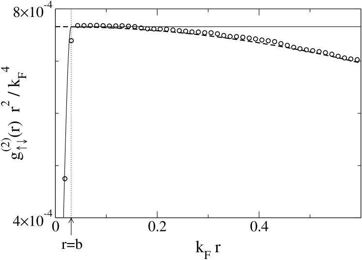
Figure 3: Pair distribution function $g_{\uparrow\downarrow}^{(2)}(r)=\langle\hat{\psi}^{\dagger}_{\uparrow}(\mathbf{r})\hat{\psi}^{\dagger}_{\downarrow}(\mathbf{0})\hat{\psi}_{\downarrow}(\mathbf{0})\hat{\psi}_{\uparrow}(\mathbf{r})\rangle$ of the homogeneous non-polarized unitary gas at zero temperature. Circles: fixed-node Monte Carlo results from Ref. Lobo et al. (2006). Solid line: analytic expression (181), where the value $\zeta=0.95$ was taken to fit the Monte Carlo results. The arrow indicates the range $b$ of the square-well interaction potential. Dashed line: analytic expression (184), with $\zeta_{e}=0.12$ Carlson et al. (2011).

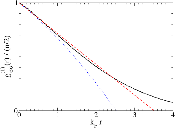
Figure 4: (Color online) One-body density matrix $g^{(1)}_{\sigma\sigma}(r)=\langle\hat{\psi}^{\dagger}_{\sigma}(\mathbf{r})\hat{\psi}_{\sigma}(\mathbf{0})\rangle$ of the homogeneous non-polarized unitary gas at zero temperature: comparison between the fixed-node Monte Carlo results from Ref. Astrakharchik et al. (2005) (black solid line) and the analytic expression (180) for the small-$k_{F}r$ expansion of $g^{(1)}_{\sigma\sigma}$ up to first order (red dashed straight line) and second order (blue dotted parabola) where we took the value $\zeta=0.95$ extracted from the Monte Carlo data for $g^{(2)}_{\uparrow\downarrow}$, see Fig. 3.

For the homogeneous non-polarized unitary gas (i.e. the spin-1/2 Fermi gas in $3D$ with $a=\infty$ and $N_{\uparrow}=N_{\downarrow}$) at zero temperature, we can compare our analytical expressions for the short-distance behavior of the one-body density matrix $g^{(1)}_{\sigma\sigma}$ and the pair distribution function $g^{(2)}_{\uparrow\downarrow}$ to the fixed-node Monte Carlo results in Astrakharchik et al. (2004, 2005); Lobo et al. (2006). In this case, $g^{(1)}_{\sigma\sigma}({\bf R}-\mathbf{r}/2,{\bf R}+\mathbf{r}/2)$ and $g^{(2)}_{\uparrow\downarrow}({\bf R}-\mathbf{r}/2,{\bf R}+\mathbf{r}/2)$ depend only on $r$ and not on $\sigma$, ${\bf R}$ and the direction of $\mathbf{r}$. Expanding the energy to first order in $1/(k_{F}a)$ around the unitary limit yields:

$$E=E_{\rm ideal}\left(\xi-\frac{\zeta}{k_{F}a}+\dots\right)$$ (179)

where $E_{\rm ideal}$ is the ground state energy of the ideal gas, $\xi$ and $\zeta$ are universal dimensionless numbers, and the Fermi wavevector is related to the density through $k_{F}=(3\pi^{2}n)^{1/3}$. Expressing $C$ in terms of $\zeta$ thanks to [Tab. II, Eqs. (2a,4a)] and Eq. (179), and inserting this into [Tab. II, Eq. (7a)], we get

$$g^{(1)}_{\sigma\sigma}(r)\simeq\frac{n}{2}\left[1-\frac{3\zeta}{10}k_{F}r-\frac{\xi}{10}(k_{F}r)^{2}+\dots\right].$$ (180)

For a finite interaction range $b$, this expression is valid for $b\ll r\ll k_{F}^{-1}$ . [Tab. IV, Eq. (4a)] yields

$$g^{(2)}_{\uparrow\downarrow}(r)\underset{k_{F}r\ll 1}{\simeq}\frac{\zeta}{40\pi^{3}}k_{F}^{4}|\phi(r)|^{2}.$$ (181)

The interaction potential used in the Monte Carlo simulations Astrakharchik et al. (2004, 2005); Lobo et al. (2006) is a square-well:

$$V(r)=-\left(\frac{\pi}{2}\right)^{2}\frac{\hbar^{2}}{mb^{2}}\,\theta(b-r)$$ (182)

The corresponding zero-energy scattering state is

$$\phi(r)=\frac{\sin\left(\frac{\pi r}{2b}\right)}{r}\ \ \mbox{for}\ \ r<b,\ \phi(r)=\frac{1}{r}\ \ \mbox{for}\ \ r>b$$ (183)

and the range $b$ was taken such that $nb^{3}=10^{-6}$ i.e. $k_{F}b=0.0309367\dots$. Thus we can assume that we are in the zero-range limit $k_{F}b\ll 1$, so that (180,181) are applicable.

Figure 3 shows that the expression (181) for $g^{(2)}_{\uparrow\downarrow}$ fits well the Monte Carlo data of Lobo et al. (2006) if one adjusts the value of $\zeta$ to $0.95$. This value is close to the value $\zeta\simeq 1.0$ extracted from (179) and the $E(1/a)$-data of Astrakharchik et al. (2004).

Using $\zeta=0.95$ we can compare the expression (180) for $g^{(1)}_{\sigma\sigma}$ with Monte Carlo data of Astrakharchik et al. (2005) without adjustable parameters. Figure 4 shows that the first order derivatives agree, while the second order derivatives are compatible within the statistical noise. This provides an interesting check of the numerical results, even though any wavefunction satisfying the contact condition [Tab. I, Eq. (1a)] leads to $g^{(1)}_{\sigma\sigma}$ and $g^{(2)}_{\uparrow\downarrow}$ functions satisfying [Tab. II, Eqs. (3a,6a)] with values of $C$ compatible with each other.

A more interesting check is provided by our expression [Tab. V, Eq.(3a)] for the subleading term in the short range behavior of $g^{(2)}_{\uparrow\downarrow}(r)$, which here reduces to

$$g^{(2)}_{\uparrow\downarrow}(r)=\frac{\zeta}{40\pi^{3}}\frac{k_{F}^{4}}{r^{2}}-\frac{\zeta_{e}}{20\pi^{3}}k_{F}^{6}+O(r)$$ (184)

where $\zeta_{e}$ is defined in Eq. (186). Remarkably, this expression is consistent with the fixed node Monte Carlo results of Lobo et al. (2006) if one uses the value of $\zeta_{e}$ of Carlson et al. (2011), see Fig. 3.

X.5 Finite-range correction in simulations and experiments

We recall that, as we have seen in Section VII, the finite-range corrections to eigenenergies are, to leading order, of the form $(\partial E/\partial r_{e})\,r_{e}$ for continuous-space models or (117) for lattice models, where the coefficients $\partial E/\partial r_{e}$, and $\partial E/\partial R_{e}$ for lattice models, are model-independent. This can be used in practice by extracting the values of these coefficients from numerical simulations, done with some convenient continuous-space or lattice models (usually a dramatic simplification of the atomic physics reality); then, knowing the value of $r_{e}$ in an experiment, one can compute the finite-range corrections present in the measurements, assuming that the universality of finite range corrections, derived in section VII for compact support potentials, also applies for multichannel $O(1/r^{6})$ models. The value of $r_{e}$ is predicted in Ref. Gao (2011) to be

$$r_{e}=-2\,R_{*}\,\left(1-\frac{a_{\rm bg}}{a}\right)^{2}\\ +\frac{4\pi\,b}{3\,\Gamma^{2}(1/4)}\,\left[\left(\frac{\Gamma^{2}(1/4)}{2\pi}-\frac{b}{a}\right)^{2}+\frac{b^{2}}{a^{2}}\right]$$ (185)

where $b$ is the van der Waals length $b=(mC_{6}/\hbar^{2})^{1/4}$, $a_{\rm bg}$ is the background scattering length and $R_{*}$ is the so-called Feshbach length Petrov (2004). We recall that the magnetic-field dependence of $a$ close to a Feshbach resonance reads $a(B)=a_{\rm bg}[1-\Delta B/(B-B_{0})]$ where $B_{0}$ is the resonance location and $\Delta B$ is the resonance width, and that $R_{*}=\hbar^{2}/(ma_{\rm bg}\mu_{b}\Delta B)$ where $\mu_{b}$ is the effective magnetic moment of the closed-channel molecule. We note that the $a$-dependent terms in the second term of (185) are $O(b^{2})$ and thus do not contribute to the leading-order correction in $b$. In contrast, the $a$-dependence of the first term of  (185) can be significant since $a_{\rm bg}$ can be much larger than $b$ (this is indeed the case for ${}^{6}{\rm Li}$) . A key assumption of Ref. Gao (2011) is that the open-channel interaction potential is well approximated by $-C_{6}/r^{6}$ down to interatomic distances $r\ll b$. This assumption is well satisfied for alkali atoms Gao (2011, 1998). Although we have not calculated the off-shell length $\rho_{e}$ explicitly, we have checked that it is finite for a $-C_{6}/r^{6}$ potential Castin (a).

As an illustration, we estimate the finite-range corrections to the non-polarized unitary gas energy in typical experiments. Similarly to (179), we have the expansion

$$E=E_{\rm ideal}\left(\xi+\zeta_{e}k_{F}r_{e}+\dots\right)$$ (186)

where $E$ and $E_{\rm ideal}$ are the ground state energies of the homogeneous Fermi gas (of fixed density $n=k_{F}^{3}/(3\pi^{2})$) for $1/a=0$ and $a=0$ respectively. The value of $\zeta_{e}$ was estimated both from fixed-node Monte Carlo and Auxiliary Field Quantum Monte Carlo to be $\zeta_{e}=0.12(3)$  Carlson et al. (2011) . The value of $r_{e}$ as given by Eq. (185) is $4.7\,{\rm nm}$ for the $B_{0}\simeq 834\,{\rm G}$ resonance of ${}^{6}{\rm Li}$ (in accordance with Simonucci et al. (2005)) and $6.7\,{\rm nm}$ for the $B_{0}\simeq 202.1\,{\rm G}$ resonance of ${}^{40}{\rm K}$. The typical value of $1/k_{F}$ is $\simeq 400\,{\rm nm}$ in Ku et al. (2012), while $1/k_{F}$ at the trap center is $\simeq 250\,{\rm nm}$ in Partridge et al. (2005) and $\simeq 100\,{\rm nm}$ in Stewart et al. (2006), which respectively leads to a finite range correction to the homogeneous gas energy:

$$\frac{\delta E}{E}\simeq 0.4\%,0.6\%\ \mbox{and}\ 2\%.$$ (187)

In the case of lithium, this type of analysis was used in Ku et al. (2012) to estimate the resulting experimental uncertainty on $\xi$.

XI Conclusion

We derived relations between various observables for $N$ spin-1/2 fermions in an external potential with zero-range or short-range interactions, in continuous space or on a lattice, in two or three dimensions. Some of our results generalize the ones of Olshanii and Dunjko (2003); Tan (2008b, a); Zhang and Leggett (2009); Tan (a); Combescot et al. (2009a): Large-momentum behavior of the momentum distribution, short-distance behavior of the pair distribution function and of the one-body density matrix, derivative of the energy with respect to the scattering length or to time, norm of the regular part of the wavefunction (defined through the behavior of the wavefunction when two particles approach each other), and, in the case of finite-range interactions, interaction energy, are all related to the same quantity $C$; and the difference between the total energy and the trapping potential energy is related to $C$ and to a functional of the momentum distribution (which is also equal to the second order term in the short-distance expansion of the one-body density matrix). We also obtained entirely new relations: The second order derivative of the energy with respect to the inverse scattering length (or to the logarithm of the scattering length in two dimensions) is related to the regular part of the wavefunctions, and is negative at fixed entropy; and the derivative of the energy with respect to the effective range $r_{e}$ of the interaction potential (or to $r_{e}^{2}$ in $2D$) is also related to the regular part, to the subleading short distance behavior of the pair distribution function, and to the subleading $1/k^{6}$ tail of the momentum distribution. We have found unexpected subtleties in the validity condition of the derived expression of this derivative in $2D$: Our expression for $\partial E/\partial(r_{e}^{2})$ applies because, for the class of interaction potentials that we have specified, the effective range squared $r_{e}^{2}$ is much larger than the true range squared $b^{2}$, than the length squared $\rho_{e}^{2}$ characterizing the low-energy $s$-wave off-shell $T$-matrix, and than the length squared $R_{1}^{2}$ characterizing the low energy $p$-wave scattering amplitude, by logarithmic factors that diverge in the zero-range limit. In $3D$, for lattice models, our expression for $\partial E/\partial r_{e}$ applies only for magic dispersion relations where an extra parameter $R_{e}$ quantifying the breaking of Galilean invariance (as predicted in Burovski et al. (2006b)) vanishes; also, the magic dispersion relation should not have cusps at the border of the first Brillouin zone otherwise the so-called Juillet effect compromises the validity of our $\partial E/\partial r_{e}$ expression for finite size systems. We have explicitly constructed such a magic relation, that may be useful to reduce lattice discretization effects in Quantum Monte Carlo simulations. We also considered models with a momentum cut-off used in Quantum Monte Carlo calculations, either in continuous space Burovski et al. (2008) or on a lattice Bulgac et al. (2006, 2008); Magierski et al. (2009, 2011): Surprisingly, in the infinite cut-off limit, the breaking of Galilean invariance survives and one does not exactly recover the unitary gas.

Applications of general relations were presented in three dimensions. For two particles in an isotropic harmonic trap, finite-interaction-range corrections were obtained, and were found to be universal up to order $r_{e}^{2}$ included in $3D$; in particular, this clarifies analytically the validity of some approximation and self-consistent equation introduced in Bolda et al. (2002); Naidon et al. (2007); Blume and Greene (2002); Chen and Gao (2007) that neglect the effect of the trapping potential within the interaction range. For the universal states of three particles with an infinite scattering length in an isotropic harmonic trap, the derivatives of the energy with respect to the inverse scattering length and with respect to the effective range were computed analytically and found to agree with available numerics. For the unitary gas in an isotropic harmonic trap, which has a $SO(2,1)$ dynamical symmetry and an undamped breathing mode of frequency $2\omega$, we have determined the relative finite-$1/a$ and finite range energy corrections within each $SO(2,1)$ ladder, which allows in the large-$N$ limit to obtain the frequency shift and the collapse time of the breathing mode. For the bulk unitary Fermi gas, existing fixed-node Monte Carlo data were checked to satisfy exact relations. Also, the finite-interaction-range correction to the unitary gas energy expected from our results to be (to leading order) model-independent and thus extractable from Quantum Monte Carlo results, was estimated for typical experiments: This quantifies one of the experimental uncertainties on the Bertsch parameter $\xi$.

The relations obtained here may be used in various other contexts. For example, the result [Tab. II, Eqs. (11a,11b)] on the sign of the second order derivative of $E$ at constant entropy is relevant to adiabatic ramp experiments Carr et al. (2004); Bartenstein et al. (2004); Stewart et al. (2006); Luo et al. (2007); Luo and Thomas (2009), and the relation [Tab. III, Eq. (8a)] allows to directly compute $C$ using determinantal diagrammatic Monte Carlo Goulko and Wingate (2010) and bold diagrammatic Monte Carlo Van Houcke et al. (2012); Fel ; Van Houcke et al. . $C$ is directly related to the closed-channel fraction in a two-channel model Braaten et al. (2008); Werner et al. (2009), which allowed to extract it Werner et al. (2009) from the experimental photoassociation measurements in Partridge et al. (2005). $C$ was measured from the tail of the momentum distribution Stewart et al. (2010). For the homogeneous gas $C$ was extracted from measurements of the equation of state Nascimbène et al. (2010b). $C$ also plays an important role in the theory of radiofrequency spectra Punk and Zwerger (2007); Baym et al. (2007); Zhang and Leggett (2009); Pieri et al. (2009); Schneider et al. ; Haussmann et al. (2009) and in finite-$a$ virial theorems Tan (2008c); Braaten and Platter (2008); Werner (2008b), as verified experimentally Stewart et al. (2010). $C$ was also extracted from the momentum tail of the static structure factor $S(k)$, which is the Fourier transform of the spin-independent pair distribution function $\langle\hat{n}(\mathbf{r})\hat{n}(\mathbf{0})\rangle$ and was measured by Bragg spectroscopy Kuhnle et al. (2010, 2011). In principle one can also measure via $S(k)$ the parameter $\zeta_{e}$ quantifying the finite range correction to the unitary gas energy, from the relation

$$\frac{\partial E}{\partial r_{e}}=-\frac{\pi\hbar^{2}}{m}\int\frac{d^{3}k}{(2\pi)^{3}}\left[S(k)-\frac{C}{4k}\right]$$ (188)

resulting from [Tab. V, Eq. (3a)]. This procedure is not hampered by the small value of $k_{F}r_{e}$ in present experiments, contrarily to the extraction of $\zeta_{e}$ from a direct measurement of the gas relative energy correction $\propto\zeta_{e}k_{F}r_{e}\lesssim 10^{-2}$.

We can think of several generalizations of the relations presented here. All relations can be extended to the case of periodic boundary conditions. The techniques used here can be applied to the one-dimensional case to generalize the relations of Olshanii and Dunjko (2003). For two-channel or multi-channel models one may derive relations other than the ones of Braaten et al. (2008); Werner et al. (2009); Zhang and Leggett (2009). Generalization of the present relations to arbitrary mixtures of atomic species, and to situations (such as indistinguishable bosons) where the Efimov effect takes place, was given in Werner and Castin (b).

Note

[Tab. II, Eq. (4b)], as well as [Tab. II, Eq. (12b)], were obtained independently by Tan Tan (c) using the formalism of Tan (a). After our preprint Werner and Castin (a) appeared, some of our $2D$ relations were tested in Bertaina and Giorgini (2011) and some of them were rederived in Valiente et al. (2011).

Appendix A Two-body scattering for the lattice model

For the lattice model defined in Sec. III.2, we recall that $\phi(\mathbf{r})$ denotes the zero-energy two-body scattering state with the normalization (9,10). In this Appendix we derive the relation (11,12) between the coupling constant $g_{0}$ and the scattering length, as well as the expressions (15,16,17,18) of $\phi(\mathbf{0})$. Some of the calculation resemble the ones in Mora and Castin (2003); Castin (b).

We consider a low-energy scattering state $\Phi_{\mathbf{q}}(\mathbf{r})$ of wavevector $q\ll b^{-1}$ and energy $E=2\epsilon_{\mathbf{q}}\simeq\hbar^{2}q^{2}/m$, i.e. the solution of the two-body Schrödinger equation (with the center of mass at rest):

$$(H_{0}+V)|\Phi_{\mathbf{q}}\rangle=E|\Phi_{\mathbf{q}}\rangle$$ (189)

where $H_{0}=\int_{D}d^{d}k/(2\pi)^{d}\,2\epsilon_{\mathbf{k}}|\mathbf{k}\rangle\langle\mathbf{k}|$ and $V=g_{0}|\mathbf{r}=\mathbf{0}\rangle\langle\mathbf{r}=\mathbf{0}|$, with the asymptotic behavior

$$\Phi_{\mathbf{q}}(\mathbf{r}) \underset{r\to\infty}{=} e^{i\mathbf{q}\cdot\mathbf{r}}+f_{\mathbf{q}}\frac{e^{iqr}}{r}+\ldots\ \ \ \ {\rm in}\ 3D$$ (190)

$$\Phi_{\mathbf{q}}(\mathbf{r}) \underset{r\to\infty}{=} e^{i\mathbf{q}\cdot\mathbf{r}}+f_{\mathbf{q}}\sqrt{\frac{2}{i\pi qr}}e^{iqr}+\ldots\ \ {\rm in}\ 2D.$$ (191)

Here $f_{\mathbf{q}}$ is the scattering amplitude , which in the present case is independent of the direction of $\mathbf{r}$ as we will see. Note that, in $2D$, the present definition corresponds to the convention (96), it differs e.g. from Petrov et al. by a factor $1/(4i)$. Also $\sqrt{i}\equiv e^{i\pi/4}$. We then have the well-known expression

$$|\Phi_{\mathbf{q}}\rangle=(1+GV)|\mathbf{q}\rangle$$ (192)

where $G\equiv(E+i0^{+}-H)^{-1}$. Since $G=G_{0}+G_{0}VG$, with $G_{0}\equiv(E+i0^{+}-H_{0})^{-1}$, Eq. (192) is equivalent to

$$|\Phi_{\mathbf{q}}\rangle=(1+G_{0}T)|\mathbf{q}\rangle$$ (193)

where the $T$-matrix is $T=V+VGV$. Indeed, (192) clearly solves (189), and one can check [using the fact that $\langle\mathbf{r}|G_{0}|\mathbf{r}=\mathbf{0}\rangle$ behaves for $r\to\infty$ as $-m/(4\pi\hbar^{2})\,e^{iqr}/r$ in $3D$ and $-(m/\hbar^{2})\sqrt{i/(8\pi qr)}e^{iqr}$ in $2D$] that (193) satisfies (190,191) with

$$f_{\mathbf{q}} = -\frac{m}{4\pi\hbar^{2}}b^{3}\langle\mathbf{r}=\mathbf{0}|T|\mathbf{q}\rangle\ \ \ \ {\rm in}\ 3D$$ (194)

$$f_{\mathbf{q}} = \frac{m}{4i\hbar^{2}}b^{2}\langle\mathbf{r}=\mathbf{0}|T|\mathbf{q}\rangle\ \ \ \ {\rm in}\ 2D.$$ (195)

Using $T=V+VGV$ and $G=G_{0}+G_{0}VG$ one gets

$$\langle\mathbf{r}=\mathbf{0}|T|\mathbf{q}\rangle=b^{-d}\left[\frac{1}{g_{0}}-\int_{D}\frac{d^{d}k}{(2\pi)^{d}}\,\frac{1}{E+i0^{+}-2\epsilon_{\mathbf{k}}}\right]^{-1}.$$ (196)

In $3D$ the scattering length in defined by $\displaystyle f_{\mathbf{q}}\underset{q\to 0}{\rightarrow}-a$, which gives the relation (11) between $a$ and $g_{0}$. In $2D$,

$$f_{\mathbf{q}}\underset{q\to 0}{=}\frac{i\pi/2}{\ln(qae^{\gamma}/2)-i\pi/2+o(1)}$$ (197)

where $a$ is by definition the $2D$ scattering length. Identifying the inverse of the right-hand-sides of Eqs. (195) and (197) and taking the real part gives the desired (12). We note that Eqs. (197,12) remain true if $q\to 0$ is replaced by the limit $b\to 0$ taken for fixed $a$.

To derive (15,16) we start from $V|\Phi_{\mathbf{q}}\rangle=T|\mathbf{q}\rangle$, which directly follows from (192). Applying $\langle\mathbf{r}=\mathbf{0}|$ on the left and using (194,195) yields

$$g_{0}\Phi_{\mathbf{q}}(\mathbf{0}) = -\frac{4\pi\hbar^{2}}{m}f_{\mathbf{q}}\ \ \ {\rm in}\ 3D$$ (198)

$$g_{0}\Phi_{\mathbf{q}}(\mathbf{0}) = \frac{4i\hbar^{2}}{m}f_{\mathbf{q}}\ \ \ {\rm in}\ 2D.$$ (199)

In $3D$, we simply have $\displaystyle\phi=-a^{-1}\underset{q\to 0}{\lim}\Phi_{\mathbf{q}}$ , and the result (15) follows. In $2D$, the situation is a bit more tricky because $\underset{q\to 0}{\lim}\Phi_{\mathbf{q}}(\mathbf{0})=0$. We thus start with $q>0$, and we will take the limit $q\to 0$ later on. At finite $q$, we define $\phi_{\mathbf{q}}(\mathbf{r})$ as being proportional to $\Phi_{\mathbf{q}}(\mathbf{r})$, and normalized by imposing the same condition (10) than at zero energy, but only for $b\ll r\ll q^{-1}$. Inserting (197) into (199) gives an expression for $\Phi_{\mathbf{q}}(\mathbf{0})$. To deduce the value of $\phi(\mathbf{0})$, it remains to calculate the $\mathbf{r}$-independent ratio $\phi_{\mathbf{q}}(\mathbf{r})/\Phi_{\mathbf{q}}(\mathbf{r})$. But for $r\gg b$ we can replace $\phi_{\mathbf{q}}(\mathbf{r})$ and $\Phi_{\mathbf{q}}(\mathbf{r})$ by their values within the zero-range model (since we also have $b\ll q^{-1}$) which we denote by $\phi_{\mathbf{q}}^{\rm ZR}(\mathbf{r})$ and $\Phi_{\mathbf{q}}^{\rm ZR}(\mathbf{r})$. The two-body Schrödinger equation

$$-\frac{\hbar^{2}}{m}\Delta\Phi_{\mathbf{q}}^{\rm ZR}=E\,\Phi_{\mathbf{q}}^{\rm ZR},\ \forall r>0$$ (200)

implies that

$$\Phi_{\mathbf{q}}^{\rm ZR}(\mathbf{r})=e^{i\mathbf{q}\cdot\mathbf{r}}+\mathcal{N}H_{0}^{(1)}(qr)$$ (201)

where $\mathcal{N}$ is a constant and $H_{0}^{(1)}$ is an outgoing Hankel function. The contact condition

$$\exists A/\ \Phi_{\mathbf{q}}^{\rm ZR}(\mathbf{r})\underset{r\to 0}{=}A\ln(r/a)+O(r)$$ (202)

together with the known short-$r$ expansion of the Hankel function Lebedev (1965) then gives

$$A=\frac{-1}{\ln(qae^{\gamma}/2)-i\pi/2}.$$ (203)

Of course we also have $\Phi_{\mathbf{q}}^{\rm ZR}/\phi_{\mathbf{q}}^{\rm ZR}=A$, which gives (16).

Finally, Eqs. (17,18) are obtained from (15,16) using the relations $d(m/(4\pi\hbar^{2}a))/d(1/g_{0})=1$ in $3D$ and $d(1/g_{0})/d(\ln a)=-m/(2\pi\hbar^{2})$ in $2D$, which are direct consequences of the relations (11,12) between $g_{0}$ and $a$.

Appendix B Derivation of a lemma

In this Appendix, we derive the lemma (33) in three dimensions, as well as its two-dimensional version (35).

Three dimensions:
By definition we have

$$\langle\psi_{1},H\psi_{2}\rangle-\langle H\psi_{1},\psi_{2}\rangle=-\frac{\hbar^{2}}{2m}\int^{\prime}d^{3}r_{1}\ldots d^{3}r_{N}\\ \sum_{i=1}^{N}\left[\psi_{1}^{*}\Delta_{\mathbf{r}_{i}}\psi_{2}-\psi_{2}\Delta_{\mathbf{r}_{i}}\psi_{1}^{*}\right].$$ (204)

Here the notation $\int^{\prime}$ means that the integral is restricted to the set where none of the particle positions coincide . We rewrite this as:

$$\langle\psi_{1},H\psi_{2}\rangle-\langle H\psi_{1},\psi_{2}\rangle=-\frac{\hbar^{2}}{2m}\sum_{i=1}^{N}\int^{\prime}\Big{(}\prod_{k\neq i}d^{3}r_{k}\Big{)}\\ \lim_{\epsilon\to 0}\int_{\{\mathbf{r}_{i}/\forall j\neq i,r_{ij}>\epsilon\}}d^{3}r_{i}\left[\psi_{1}^{*}\Delta_{\mathbf{r}_{i}}\psi_{2}-\psi_{2}\Delta_{\mathbf{r}_{i}}\psi_{1}^{*}\right].$$ (205)

We note that this step is not trivial to justify mathematically. The order of integration has been changed and the limit $\epsilon\to 0$ has been exchanged with the integral over $\mathbf{r}_{i}$. We expect that this is valid in the presently considered case of equal mass fermions, and more generally provided the wavefunctions are sufficiently regular in the limit where several particles tend to each other.

Since the integrand is the divergence of $\psi_{1}^{*}\nabla_{\mathbf{r}_{i}}\psi_{2}-\psi_{2}\nabla_{\mathbf{r}_{i}}\psi_{1}^{*}$, the divergence theorem gives

$$\langle\psi_{1},H\psi_{2}\rangle-\langle H\psi_{1},\psi_{2}\rangle=\frac{\hbar^{2}}{2m}\sum_{i=1}^{N}\int^{\prime}\Big{(}\prod_{k\neq i}d^{3}r_{k}\Big{)}\\ \lim_{\epsilon\to 0}\sum_{j,j\neq i}\ \oiint_{S_{\epsilon}(\mathbf{r}_{j})}\left[\psi_{1}^{*}\nabla_{\mathbf{r}_{i}}\psi_{2}-\psi_{2}\nabla_{\mathbf{r}_{i}}\psi_{1}^{*}\right]\cdot\mathbf{dS}$$ (206)

where the surface integral is for $\mathbf{r}_{i}$ belonging to the sphere $S_{\epsilon}(\mathbf{r}_{j})$ of center $\mathbf{r}_{j}$ and radius $\epsilon$, and the vector area $\mathbf{dS}$ points out of the sphere. We then expand the integrand by using the contact condition, in the limit $r_{ij}=\epsilon\to 0$ taken for fixed $\mathbf{r}_{j}$ and fixed $(\mathbf{r}_{k})_{k\neq i,j}$. Using $\mathbf{R}_{ij}=\mathbf{r}_{j}+\epsilon\mathbf{u}/2$ with $\mathbf{u}\equiv(\mathbf{r}_{i}-\mathbf{r}_{j})/r_{ij}$ we get

$$\!\!\!\psi_{n}\!\!\!\! \underset{\epsilon\to 0}{=} \!\!\!\!\left(\frac{1}{\epsilon}-\frac{1}{a_{n}}\right)A_{ij}^{(n)}+\frac{1}{2}\mathbf{u}\cdot\nabla_{\mathbf{R}_{ij}}A_{ij}^{(n)}+O(\epsilon)$$ (207)

$$\!\!\!\nabla_{\mathbf{r}_{i}}\psi_{n}\!\!\!\! \underset{\epsilon\to 0}{=} \!\!\!\!-\frac{\mathbf{u}}{\epsilon^{2}}A_{ij}^{(n)}\!\!\!+\!\frac{1}{2\epsilon}\!\left[\nabla_{\mathbf{R}_{ij}}A_{ij}^{(n)}\!\!-\!\mathbf{u}(\mathbf{u}\cdot\!\nabla_{\mathbf{R}_{ij}}A_{ij}^{(n)})\right]\!\!+\!O(1)$$

where $n$ equals $1$ or $2$, and the functions $A_{ij}^{(n)}$ and $\nabla_{\mathbf{R}_{ij}}A_{ij}^{(n)}$ are taken at $\left(\mathbf{r}_{j},(\mathbf{r}_{k})_{k\neq i,j}\right)$. This simply gives

$$\oiint_{S_{\epsilon}(\mathbf{r}_{j})}\left[\psi_{1}^{*}\nabla_{\mathbf{r}_{i}}\psi_{2}-\psi_{2}\nabla_{\mathbf{r}_{i}}\psi_{1}^{*}\right]\cdot\mathbf{dS}\underset{\epsilon\to 0}{=}4\pi\left(\frac{1}{a_{1}}-\frac{1}{a_{2}}\right)\\ \times A_{ij}^{(1)\,*}A_{ij}^{(2)}+O(\epsilon)$$ (209)

because the leading order term cancels and most angular integrals vanish. Inserting this into (206) gives the desired lemma (33).

Two dimensions:
The derivation is analogous to the $3D$ case. In (206), the double integral on the sphere of course has to be replaced by a simple integral on the circle. Instead of (207,LABEL:eq:grad_psi_n_3D), we now obtain, from the $2D$ contact condition [Tab. I, Eq. (1b)],

$$\psi_{n} \underset{\epsilon\to 0}{=} \ln(\epsilon/a_{n})\ A_{ij}^{(n)}+O(\epsilon\ln\epsilon)$$ (210)

$$\nabla_{\mathbf{r}_{i}}\psi_{n} \underset{\epsilon\to 0}{=} \frac{\mathbf{u}}{\epsilon}A_{ij}^{(n)}+O(\ln\epsilon),$$ (211)

which gives

$$\oint_{S_{\epsilon}(\mathbf{r}_{j})}\left[\psi_{1}^{*}\nabla_{\mathbf{r}_{i}}\psi_{2}-\psi_{2}\nabla_{\mathbf{r}_{i}}\psi_{1}^{*}\right]\cdot\mathbf{dS}\underset{\epsilon\to 0}{=}2\pi\ln(a_{2}/a_{1})\\ \times A_{ij}^{(1)\,*}A_{ij}^{(2)}+O(\epsilon\ln^{2}\epsilon)$$ (212)

and yields the lemma (35).

Appendix C Zero-range limit of the lattice model’s contact

In this appendix, we show that our definition [Tab. III, Eqs. (1a,1b)] of the contact operator $\hat{C}$ within the lattice model agrees in the zero-range limit $b\to 0$ with the way [Tab. II, Eq. (1)] $C$ is usually defined within the zero-range model.

C.1 Stationary state

Let us first consider an eigenstate $|\psi\rangle$ of the zero-range model with an energy $E$. Let $|\psi_{b}\rangle$ denote the eigenstate of the lattice model which tends to $|\psi\rangle$ when $b\to 0$, and $E_{b}$ the corresponding eigenenergy. Then, $C_{b}\equiv\langle\psi_{b}|\hat{C}|\psi_{b}\rangle$ tends to the contact $C$ of the state $\psi$ [defined in Tab. II, Eq. (1)] when $b\to 0$. Indeed, $C$ is related to $dE/d(-1/a)$ by [Tab. II, Eq. (4a)]; $C_{b}$ is related to $dE_{b}/d(-1/a)$ by [Tab. II, Eq. (4a)]; and the function $E_{b}(1/a)$ should tend smoothly to $E(1/a)$ when $b\to 0$.

C.2 Arbitrary pure state

We now consider any pure state $|\psi\rangle$ satisfying the contact condition [Tab. I, Eq. (1a)]. We will show that $C_{b}\equiv\langle\psi_{b}|\hat{C}|\psi_{b}\rangle$ tends to the contact $C$ of the state $|\psi\rangle$ [defined in Tab. II, Eq. (1)] when $b\to 0$, where $|\psi_{b}\rangle$ is defined as follows: Writing $|\psi\rangle$ as a linear combination $\sum_{n}c^{(n)}|\psi^{(n)}\rangle$ of the zero-range model’s eigenstates $|\psi^{(n)}\rangle$, we define the linear combination $|\psi_{b}\rangle\equiv\sum_{n}c^{(n)}|\psi_{b}^{(n)}\rangle$ of the lattice-model’s eigenstates $|\psi_{b}^{(n)}\rangle$.

We consider only the $3D$ case, the derivation being almost identical in $2D$. Let $A$ and $A^{(n)}$ denote the regular parts of $\psi$ and $\psi^{(n)}$ [defined by the contact condition Tab. I, Eq. (1a)], and $A_{b}$ and $A_{b}^{(n)}$ denote the regular parts of $\psi_{b}$ and $\psi_{b}^{(n)}$ [defined by (19)]. Linearity immediately gives $A=\sum_{n}c^{(n)}A^{(n)}$ and $A_{b}=\sum_{n}c^{(n)}A_{b}^{(n)}$, as well as $C_{b}=\sum_{n,m}(c^{(n)}_{b})^{*}c^{(m)}_{b}\langle\psi^{(n)}_{b}|\hat{C}|\psi^{(m)}_{b}\rangle$. Expressing $\hat{C}$ in terms of $H_{\rm int}$ thanks to [Tab. III, Eq. (2)], and using the lemma (56) as well as (15), we get $\langle\psi^{(n)}_{b}|\hat{C}|\psi^{(m)}_{b}\rangle=(4\pi)^{2}\,(A^{(n)}_{b},A^{(m)}_{b})$. When $b\to 0$, we expect that this last quantity tends to $(4\pi)^{2}\,(A^{(n)},A^{(m)})$ because $A_{b}^{(n)}\to A^{(n)}$ [see (19) and the discussion thereafter]. Thus $C_{b}$ indeed tends to $C$.

Appendix D Spectral effect of the trapping potential within the interaction range

The motivation of this Appendix is to justify the fact that, in Eq. (88) and in its equivalent form in $2D$ for a $N$-body problem, we have neglected the effect of the trapping potential within the interaction range. In the case of an isotropic harmonic trap, the exact form of Eq. (88) contains the external potential term $\frac{1}{4}m\omega^{2}r_{ij}^{2}$. This issue is thus mappable to the two-body problem in a trap with a finite range interaction, which was the object of numerous studies in $3D$ Blume and Greene (2002); Bolda et al. (2002); Naidon et al. (2007); Chen and Gao (2007) that have however not analytically quantified the effect of the trapping potential within the interaction range. After elimination of the center of mass motion and restriction to a zero angular momentum, one faces the $3D$ or $2D$ eigenvalue problem

$$E\psi(r)=-\frac{\hbar^{2}}{m}\Delta\psi(r)+\left[\frac{1}{4}m\omega^{2}r^{2}+V(r;b)\right]\psi(r)$$ (213)

with the conditions that $\psi$ diverges neither in $r=0$ nor at infinity. The rotationally invariant compact support potential $V(r;b)$ of range $b$ is of the minimal depth ensuring a fixed scattering length $a$ (as discussed in subsection VII.2). In the limit $b\to 0$, where $E$ converges to a finite value, we show that neglecting the effect of the trapping potential within the interaction range $r\leq b$, as done in subsection VII.1, introduces on the eigenenergy $E$ an error $O(b^{3})$ in $3D$ and $O[b^{4}\ln^{2}(a/b)]$ in $2D$, which thus does not affect the results [Tab. V, Eqs. (1a,1b)].

The starting point is the Hellmann-Feynman theorem, with $\psi$ real and normalized to unity:

$$\frac{dE}{db}=\int d^{d}r\,\psi^{2}(r)\,\partial_{b}V(r;b).$$ (214)

To reexpress this integral in a more operational way, we introduce the solution $\tilde{\psi}(r)$ of Schrödinger’s equation with the same eigenvalue $E$ but for the interaction potential $V(r;\tilde{b})$ of a different range $\tilde{b}$. This solution $\tilde{\psi}(r)$ remains finite in $r=0$ but it diverges at infinity and cannot be $L^{2}$-normalized. In what follows we take a convenient normalization of $\tilde{\psi}$ such that $\lim_{\tilde{b}\to b}\tilde{\psi}=\psi$.

We multiply Schrödinger’s equation for $\psi$ (respectively $\tilde{\psi}$) by $\tilde{\psi}$ (respectively $\psi$) and we integrate the difference of the two resulting equations over the domain $r<R$. Using the divergence theorem, the Wronskian $W(R)$ appears,

$$W(r)\equiv\tilde{\psi}(r)\psi^{\prime}(r)-\psi(r)\tilde{\psi}^{\prime}(r).$$ (215)

For $r>b,\tilde{b}$, the Wronskian satisfies the differential equation $W^{\prime}(r)=-\frac{d-1}{r^{d-1}}W(r)$, so that, for large $R$, $W(R)=\frac{w}{R^{d-1}}$ and

$$w=\frac{m}{\hbar^{2}}\int_{0}^{+\infty}\!\!\!dr\,r^{d-1}[V(r;b)-V(r;\tilde{b})]\tilde{\psi}(r)\psi(r).$$ (216)

Turning back to the Hellmann-Feynman formula (214), we obtain the exact relation

$$\frac{dE}{db}=\frac{2(d-1)\pi\hbar^{2}}{m}\lim_{\tilde{b}\to b}\frac{w}{b-\tilde{b}}$$ (217)

It remains to calculate $w$ treating perturbatively the trapping potential within the interaction range.

To zeroth order, one neglects the trapping potential for $r\leq b$ [or $r\leq\tilde{b}$ for $\tilde{\psi}$], so that $\psi^{(0)}(r)=\mathcal{A}\chi(r)$, where $\chi$ is the scattering state of energy $E$ for $V(r;b)$. Taking for simplicity $E>0$, we set $E=\hbar^{2}k^{2}/m$, $k>0$, and $\chi$ is normalized as in Eqs. (89,95). Note that $\mathcal{A}$ is then fully specified by the continuous matching of $\psi^{(0)}$ in $r=b$ to the outer solution in the trapping potential (that can be expressed in terms of Whittaker functions, see subsection X.1) and by the fact that $\psi$ is normalized to unity. We also have $\tilde{\psi}^{(0)}(r)=\mathcal{A}\tilde{\chi}(r)$ for $r\leq\tilde{b}$, where $\tilde{\chi}$ is the scattering state of energy $E$ for $V(r;\tilde{b})$ and the same prefactor $\mathcal{A}$ was taken for convenience. The zeroth-order Wronskian $W^{(0)}$ can then be calculated explicitly, in particular using relations 8.477(1) and 8.473(4,5) of Gradshteyn and Ryzhik (1994). We use Eqs. (93,97), with $\ldots=O[(kb)^{4}\ln(a/b)]$ in (97) [as we have checked for the square well], to obtain

$$\left(\frac{dE}{db}\right)^{(0)} \stackrel{{\scriptstyle 3D}}{{=}} 2\pi E\mathcal{A}^{2}\frac{dr_{e}}{db}+O(b^{2})$$ (218)

$$\left(\frac{dE}{db}\right)^{(0)} \stackrel{{\scriptstyle 2D}}{{=}} \pi E\mathcal{A}^{2}\frac{d}{db}(r_{e}^{2})+O[b^{3}\ln(a/b)]$$ (219)

We have checked that the $b\to 0$ limit of these relations coincide with [Tab. V, Eqs. (1a,1b)].

To first order, we treat the trapping potential perturbatively within the interaction range. We rescale the distance by $b$, so that $\psi^{(1)}(r)=f(x)$, and $\chi(r)=\mathcal{N}u(x)$, where $x=r/b$ and the function $u(x)$ is normalized by the condition $u(0)=1$. The function $f$ solves the inhomogeneous Schrödinger equation:

$$\!\!\!\!\!\!f^{\prime\prime}(x)+\frac{d-1}{x}f^{\prime}(x)+\left[k^{2}b^{2}\!-\!\frac{mb^{2}}{\hbar^{2}}V(bx;b)\right]\!f(x)=\mathcal{F}x^{2}u(x)\\ \mbox{with}\ \mathcal{F}=\frac{1}{4}\mathcal{A}\mathcal{N}\frac{m^{2}\omega^{2}}{\hbar^{2}}b^{4}$$ (220)

The function $u(x)$ is a solution of the corresponding homogeneous equation. A second solution $v(x)$ can be constructed, that diverges for $x\to 0$. It is of the form $v(x)=-\frac{u(x)}{x}+Z_{3}(x)$ with $Z_{3}(x)=O(x)$ for $x\to 0$ in $3D$, and $v(x)=u(x)\ln x+Z_{2}(x)$ with $Z_{2}(x)=O(x^{2})$ for $x\to 0$ in $2D$. More precisely, one has $Z_{d}(x)=u(x)\int_{0}^{x}dy\,y^{1-d}[-1+1/u^{2}(y)]$. Since the expression between square brackets in the left-hand side of Eq. (220) is $O(1)$, $u(x)$ and $Z_{d}(x)$ are $O(1)$ for $x\leq 1$. A first consequence is that the factor $\mathcal{N}$ scales as $1/b$ in $3D$ and as $\ln(a/b)$ in $2D$ . A second consequence is that, both in two and three dimensions,

$$\psi^{(1)}(b)\ \mbox{and}\ b\,\psi^{(1)^{\prime}}\!(b)=O(\mathcal{F}).$$ (221)

This can be seen with the method of variation of constants, where one sets $(f(x),f^{\prime}(x))=\alpha(x)(u(x),u^{\prime}(x))+\beta(x)(v(x),v^{\prime}(x))$, with the boundary conditions $\alpha(0)=0$ (so that $\psi^{(1)}$ does not duplicates the zeroth order solution) and $\beta(0)=0$ (so that $\psi^{(1)}$ does not diverge in $r=0$). This leads to

$$\alpha(x) = -\mathcal{F}\int_{0}^{x}dy\,y^{d+1}u(y)v(y)$$ (222)

$$\beta(x) = \mathcal{F}\int_{0}^{x}dy\,y^{d+1}u^{2}(y)$$ (223)

Similar results hold for $\tilde{\psi}^{(1)}$. From Eq. (221) and its counterpart for $\tilde{\psi}^{(1)}(\tilde{b})$, $\tilde{\psi}^{(1)^{\prime}}(\tilde{b})$, we can estimate the variation of the Wronskian $W(R)$ for $R$ close to $b,\tilde{b}$, and thus the variation $w^{(1)}$ of $w$ due to the trapping potential. Dividing by $b-\tilde{b}$ and taking the limit $\tilde{b}\to b$ as in Eq. (217) amounts to taking a derivative with respect to $\tilde{b}$, which gives an additional factor $O(1/b)$. Finally the error $\delta E$ introduced on the eigenenergy by the neglection of the trapping potential within the interaction range is bounded in the zero range limit $b\to 0$ as

$$\delta E \stackrel{{\scriptstyle 3D}}{{=}} O(m\omega^{2}b^{3}\mathcal{A}^{2})$$ (224)

$$\delta E \stackrel{{\scriptstyle 2D}}{{=}} O[m\omega^{2}b^{4}\mathcal{A}^{2}\ln^{2}(a/b)]$$ (225)

where the factor $\mathcal{A}$ converges to a finite, energy-dependent value for $b\to 0$.

Appendix E Low-energy $T$-matrix parameters in $2D$

We derive the hierarchy (109,110,111) for a $2D$ non-positive minimal-depth potential of finite range $b$, $V(r)=\frac{\hbar^{2}k_{0}^{2}}{m}v(r/b)$, for $b\to 0$ and $k_{0}$ adjusted to have a constant $s$-wave scattering length $a$. The key point is then that $k_{0}b\to 0$ (differently from $3D$).

In the $s$-wave channel, we write the zero-energy scattering wavefunction as $\psi(r)=f(x)$, with $x=r/b$. The function $f$ solves $f^{\prime\prime}(x)+\frac{1}{x}f^{\prime}(x)=(k_{0}b)^{2}v(x)f(x)$ and it is normalized as $f(0)=1$. We expand $f(x)$ in powers of $(k_{0}b)^{2}$. To zeroth order, $f_{0}(x)=1$. To first order, $f_{1}^{\prime\prime}+\frac{1}{x}f_{1}^{\prime}=(k_{0}b)^{2}v(x)$, with $f_{1}(0)=0$. This is integrated with the method of variation of constants, $f_{1}(x)=\alpha(x)+\beta(x)\ln x$ and $f_{1}^{\prime}(x)=\beta(x)/x$:

$$\alpha(x) = -(k_{0}b)^{2}\int_{0}^{x}dy\,y\,v(y)\ln y$$ (226)

$$\beta(x) = (k_{0}b)^{2}\int_{0}^{x}dy\,y\,v(y).$$ (227)

Expressing that $f_{1}(x)\simeq\beta(+\infty)\ln(r/a)$ at infinity gives

$$-\frac{1}{\ln(a/b)}\simeq\frac{\beta(+\infty)}{1+\alpha(+\infty)}\simeq\frac{m}{\hbar^{2}}\int_{0}^{+\infty}dr\,r\,V(r)$$ (228)

and further using Eq. (106) leads to

$$\frac{1}{2}\rho_{e}^{2}\sim b^{2}\int_{0}^{+\infty}\!\!\!\!dx\,x\left[\frac{\beta(x)-\beta(+\infty)}{\beta(+\infty)}\ln x+\frac{\alpha(x)-\alpha(+\infty)}{\beta(+\infty)}\right]$$ (229)

Integration by parts then gives Eq. (110). Using Eqs. (105,228,229) and realizing that $\phi(r)+\ln(r/a)=\frac{2}{\beta(+\infty)}+O(1)$ for $b\to 0$ with $0<r/b\leq 1$ fixed, gives Eq. (109). Reproducing this perturbative expansion with the same $v(x)$ in the $l$-wave, one gets

$$R_{l}^{2l}\underset{b\to 0}{\sim}\left(\frac{b^{l}}{2^{l}l!}\right)^{2}\frac{1}{\ln(a/b)}\frac{\int_{0}^{\infty}dx\,x^{2l+1}v(x)}{\int_{0}^{\infty}dx\,x\,v(x)}$$ (230)

This relation for $l=1$, combined with Eq. (110), gives Eq. (111).

Appendix F Some maths for the Juillet effect

Here, in the context of the Juillet effect for lattice models, we justify the expansion (133). The quantity $R_{1}$ defined in Eq. (130) may be expressed in terms of the difference between an integral and a $3D$ Riemann sum. We are then guided by the following type of results: If $f(\mathbf{x})$ is a $C^{\infty}$ function inside the cube $B=[-1/2,1/2]^{3}$, then for $\varepsilon=1/(2N+1)$, with the integer $N\to+\infty$:

$$\int_{B}d^{3}x\,f(\mathbf{x})-\varepsilon^{3}\sum_{\mathbf{n}}f(\varepsilon\mathbf{n})=\frac{\varepsilon^{2}}{24}\int_{B}d^{3}x\,\Delta f(\mathbf{x})+O(\varepsilon^{4})$$ (231)

where $\Delta f$ is the Laplacian of $f$ and the sum over $\mathbf{n}$ ranges over $\{-N,\ldots,N\}^{3}$. To show this lemma, we introduce the short-hand notation $S[f]$ for the left-hand side of (231) and we pave $B$ with little cubes of volume $\varepsilon^{3}$ and of centers $\varepsilon\mathbf{n}$:

$$S[f]=\sum_{\mathbf{n}}\varepsilon^{3}\int_{B}d^{3}x[f(\varepsilon\mathbf{n}+\varepsilon\mathbf{x})-f(\varepsilon\mathbf{n})].$$ (232)

Then we use the fourth-order Taylor-Lagrange formula for $f$ restricted to the line connecting $\varepsilon\mathbf{n}$ to $\varepsilon\mathbf{n}+\varepsilon\mathbf{x}$: $f(\varepsilon\mathbf{n}+\varepsilon\mathbf{x})-f(\varepsilon\mathbf{n})=\frac{\varepsilon^{2}}{2}\sum_{i,j}x_{i}x_{j}\partial_{i}\partial_{j}f(\varepsilon\mathbf{n})+\mbox{odd}+O(\varepsilon^{4})$ where “odd” stands for terms that are linear and cubic in the components of $\mathbf{x}$, and $O(\varepsilon^{4})$ results from the fact that the fourth-order derivatives of $f$ are uniformly bounded on $B$. Integration over $\mathbf{x}$ inside the cube $B$ eliminates the odd terms, and the $i\neq j$ quadratic terms, so that

$$S[f]=\frac{\varepsilon^{5}}{24}\sum_{\mathbf{n}}\left[\Delta f(\varepsilon\mathbf{n})+O(\varepsilon^{2})\right].$$ (233)

A Riemann sum thus deviates from the integral by $O(\varepsilon^{2})$, for a $C^{\infty}$ integrand. Applying this conclusion to Eq. (233), where $\Delta f$ is $C^{\infty}$, we obtain the desired Eq. (231). This result is however not immediate to apply to the quantity $R_{1}$ because the integrand of $R_{1}$ is singular in $\mathbf{k}=\mathbf{0}$. We thus use several steps.

We first consider the quantity $R_{1}$ for a quadratic dispersion relation that is cut in a smooth way: One twice replaces $1/(2\epsilon_{\mathbf{k}})$ in Eq. (130) by $\phi(\mathbf{k}b/2\pi)/(\hbar^{2}k^{2}/m)$ where $\phi(\mathbf{x})$ is a $C^{\infty}$ rotationally invariant function, equal to $1$ in $\mathbf{x}=\mathbf{0}$, and of compact support included inside $B\equiv[-1/2,1/2]^{3}$ (which allows to replace the set $D$ by $\mathbb{R}^{3}$ in the integration and in the summation). After the change of variable $\mathbf{k}=2\pi\mathbf{x}/L$, we decompose $\mathbb{R}^{3}$ as a collection of cubes of size unity (as in Pricoupenko and Castin (2007b)), to obtain

$$\!\!\!\!\!\frac{h^{2}L}{m}R_{1}^{\phi}=\!\!\!\!\sum_{\mathbf{n}\in\mathbb{Z}^{3*}}\!\int_{B}\!\!\!d^{3}x\!\left[\frac{\phi(\varepsilon\mathbf{n}+\varepsilon\mathbf{x})}{(\mathbf{n}+\mathbf{x})^{2}}-\frac{\phi(\varepsilon\mathbf{n})}{n^{2}}\right]+\!\int_{B}\!\!d^{3}x\frac{\phi(\varepsilon\mathbf{x})}{x^{2}}$$ (234)

with $h=2\pi\hbar$ is Planck’s constant and $\varepsilon\equiv b/L$ is the small parameter. As shown in Pricoupenko and Castin (2007b), the right-hand side of Eq. (234) has a finite limit when $\varepsilon\to 0$, here called $\mathcal{C}\simeq 8.91363$, that one can obtain by taking $\varepsilon$ to zero inside the sum and the integral, which amounts to replacing $\phi$ by unity. The deviation of Eq. (234) from its $\varepsilon\to 0$ limit can thus be exactly written as $\{S[f]+\varepsilon^{3}f(\mathbf{0})\}/\varepsilon$, with $S[f]=\varepsilon^{3}\sum_{\mathbf{n}\in\mathbb{Z}^{3}}\int_{B}d^{3}x[f(\varepsilon\mathbf{n}+\varepsilon\mathbf{x})-f(\varepsilon\mathbf{n})]$, that we treat as we did for Eq. (232). Here $f(\mathbf{x})=[\phi(\mathbf{x})-1]/x^{2}$ (extended by continuity to $\mathbf{x}=\mathbf{0}$) is a $C^{\infty}$ function since $\phi$ is rotationally invariant. In the fourth-order Taylor-Lagrange formula, $O(\varepsilon^{4})$ is replaced with the more accurate $O(\frac{\varepsilon^{4}}{(1+\varepsilon^{2}n^{2})^{3}})$, due to the fact that the fourth order derivatives of $f(\mathbf{x})$ are uniformly bounded and decrease as $1/x^{6}$ at infinity. The integral of the Laplacian of $f$ appears as in Eq. (231), except that is in integrated over the whole $\mathbb{R}^{3}$ space, which gives zero. We finally obtain

$$\frac{h^{2}L}{m}R_{1}^{\phi}\underset{b\to 0}{=}\mathcal{C}+\left(\frac{b}{L}\right)^{2}\lim_{\mathbf{x}\to\mathbf{0}}\frac{\phi(\mathbf{x})-1}{x^{2}}+O(b/L)^{3}.$$ (235)

Turning back to the lattice model, we now evaluate how $R_{1}$ deviates from its $b\to 0$ limit for the uncut parabolic dispersion relation $\mathbf{k}\to\hbar^{2}k^{2}/(2m)$. The difference between the smoothly-cut $R_{1}^{\phi}$ and the uncut $R_{1}^{\rm parab}$ (times $h^{2}L/m$) is now of the form $\varepsilon^{2}f(\mathbf{0})$ plus $\frac{1}{\varepsilon}$ times the difference $S[f]$ between an integral and a Riemann sum, with $f(\mathbf{x})=[\phi(\mathbf{x})-1]/x^{2}$ as before is $C^{\infty}$. We then use the result (231), the key point being that the integration domain is $B$ (rather than the whole space), so that the integral of the Laplacian of $f$ over $B$ gives a non-zero surface contribution, equals to the flux of the gradient of $f$ through the surface of $B$. This leads to Eq. (133) for the particular case of the parabolic dispersion relation. The surface term can be evaluated explicitly, as in subsection VII.2, from the integral evaluated in polar coordinates:

$$\int_{[-1,1]^{2}}\frac{dxdy}{(1+x^{2}+y^{2})^{2}}=\sqrt{8}\arcsin\frac{1}{\sqrt{3}}$$ (236)

Finally, we consider a general dispersion relation (132), with $\eta_{\mathbf{x}}=\frac{1}{2}x^{2}+O(x^{4})$ for $\mathbf{x}\to\mathbf{0}$. One can consider the difference between the corresponding $R_{1}$ and $R_{1}^{\rm parab}$. The corresponding function $f(\mathbf{x})=1/(2\eta_{\mathbf{x}})-1/x^{2}$ is then not $C^{\infty}$ in $\mathbf{x}=\mathbf{0}$. E.g. for the Hubbard model, $\eta_{\mathbf{x}}=[3-\sum_{i}\cos 2\pi x_{i}]/(2\pi)^{2}$ is not rotationally invariant and $f(\mathbf{x})$ behaves as $\sum_{i}x_{i}^{4}/x^{4}$ at low $x$, its $\mathbf{x}\to\mathbf{0}$ limit depends on the direction of $\mathbf{x}$. This limiting behavior is however scaling invariant, a feature that holds for a general dispersion relation. The $n^{\rm th}$ order derivatives of $f$ are then $O(1/x^{n})$ for $\mathbf{x}\to\mathbf{0}$. For this class of functions, we introduce $S^{*}[f]$ defined as $S[f]$ in Eq. (231) except that one excludes the term $\mathbf{n}=\mathbf{0}$ in the sum. This implies that in the equivalent of Eq. (232), there is an isolated contribution, the integral of $f$ over $\varepsilon B$, which is $O(\varepsilon^{3})$ and negligible. Then reproducing the analysis with the fourth-order Taylor-Lagrange formula we obtain

$$S^{*}[f]=\frac{\varepsilon^{2}}{24}\int_{B}d^{3}x\,\Delta f(\mathbf{x})+O(\varepsilon^{3}).$$ (237)

As $\frac{h^{2}L}{m}(R_{1}-R_{1}^{\rm parab})=S^{*}[f]/\varepsilon$, we obtain Eq. (133).

Appendix G Isentropic derivatives of the mean energy in the canonical ensemble

One considers a system with a Hamiltonian $H(\lambda)$ depending on some parameter $\lambda$, and at thermal equilibrium in the canonical ensemble at temperature $T$, with a density operator $\rho=\exp(-\beta H)/Z$. In terms of the partition function $Z(T,\lambda)=\mbox{Tr}\,e^{-\beta H(\lambda)}$, with $\beta=1/(k_{B}T)$, one has the usual relations for the free energy $F$, the mean energy $\bar{E}=\mbox{Tr}(\rho H)$ and the entropy $S=-k_{B}\mbox{Tr}(\rho\ln\rho)$:

$$F(T,\lambda) = -k_{B}T\ln Z(T,\lambda)$$ (238)

$$F(T,\lambda) = \bar{E}(T,\lambda)-TS(T,\lambda)$$ (239)

$$\partial_{T}F(T,\lambda) = -S(T,\lambda).$$ (240)

One now varies $\lambda$ for a fixed entropy $S$. The temperature is thus a function $T(\lambda)$ of $\lambda$ such that $S(T(\lambda),\lambda)=\mbox{constant}$. The derivatives of the mean energy for fixed entropy are $(\frac{d\bar{E}}{d\lambda})_{S}\equiv\frac{d}{d\lambda}[\bar{E}(T(\lambda),\lambda)]$ and $(\frac{d^{2}\bar{E}}{d\lambda^{2}})_{S}\equiv\frac{d^{2}}{d\lambda^{2}}[\bar{E}(T(\lambda),\lambda)]$. Writing (239) for $T=T(\lambda)$ and taking the first order and the second order derivatives of the resulting equation with respect to $\lambda$, one finds

$$\left(\frac{d\bar{E}}{d\lambda}\right)_{S}\!\!\!\! = \!\!\partial_{\lambda}F(T(\lambda),\lambda)$$ (241)

$$\left(\frac{d^{2}\bar{E}}{d\lambda^{2}}\right)_{S}\!\!\!\! = \!\!\partial_{\lambda}^{2}F(T(\lambda),\lambda)-\frac{\left[\partial_{T}\partial_{\lambda}F(T(\lambda),\lambda)\right]^{2}}{\partial_{T}^{2}F(T(\lambda),\lambda)}$$ (242)

It remains to use (238) to obtain a microscopic expression of the above partial derivatives of $F$, from the partition function expressed as a sum $Z=\sum_{n}e^{-\beta E_{n}}$ over the eigenstates $n$ of the Hamiltonian:

$$\partial_{\lambda}F(T,\lambda) = \overline{\frac{dE}{d\lambda}}$$ (243)

$$\partial_{\lambda}^{2}F(T,\lambda) = \overline{\frac{d^{2}E}{d\lambda^{2}}}-\beta\,\mbox{Var}\!\left(\frac{dE}{d\lambda}\right)$$ (244)

$$\partial_{T}^{2}F(T,\lambda) = -\frac{\mbox{Var}E}{k_{B}T^{3}}$$ (245)

$$\partial_{T}\partial_{\lambda}F(T,\lambda) = \frac{\mbox{Cov}(E,dE/d\lambda)}{k_{B}T^{2}}.$$ (246)

Here the expectation value $\overline{(\ldots)}$ stands for a sum over the eigenenergies with the canonical probability weights, and Var and Cov are the corresponding variance and covariance, e.g. $\mbox{Cov}(E,dE/d\lambda)\!\!\equiv\!\!\sum_{n}E_{n}\frac{dE_{n}}{d\lambda}\frac{e^{-\beta E_{n}}}{Z}-\overline{E}\ \overline{\frac{dE}{d\lambda}}$. Insertion of (243) into (241) gives (146). Insertion of (244,245,246) into (242) gives (150).

Appendix H Non-zero $1/a$ and $r_{e}$ corrections within a ladder of the trapped unitary gas

For $N$ spin-1/2 fermions at the unitary limit in an isotropic harmonic trap, there is separability of the wavefunction in internal hyperspherical coordinates Werner and Castin (2006b):

$$\psi(\mathbf{r}_{1},\ldots,\mathbf{r}_{N})=\psi_{\rm cm}(\mathbf{C})R^{-(3N-5)/2}F(R)\Phi(\Omega)$$ (247)

where $\mathbf{C}$ is the center-of-mass location of the $N$ fermions, $R$ is the hyperradius and $\Omega$ is a set of $3N-4$ hyperangles constructed from the Jacobi coordinates (see e.g. Castin and Werner ). One has the general formulas $\mathbf{C}=\sum_{i=1}^{N}m_{i}\mathbf{r}_{i}/M$ and $R^{2}=\sum_{i=1}^{N}m_{i}(\mathbf{r}_{i}-\mathbf{C})^{2}/\bar{m}$, where $M=\sum_{i=1}^{N}m_{i}$ is the total mass, $\bar{m}$ an arbitrary mass unit, and $m_{i}$ is the mass of particle $i$ (here equal to $m$). We shall not need the expression of the hyperangles. Eq. (247) is due to the separability of the non-interacting Hamiltonian in a harmonic trap, and to the fact that the Bethe-Peierls contact condition do not break this separability for $1/a=0$. One finds that $\Phi(\Omega)$ is an eigenstate of the Laplacian on the unit sphere of dimension $3N-4$, with contact conditions. Corresponding eigenvalues are conveniently written as $(\frac{3N-5}{2})^{2}-s^{2}$, $s>0$. In the $N$-body case, $s$ is not known analytically. On the contrary, $F(R)$ solves a simple $2D$ Schrödinger-like equation

$$(E-E_{\rm cm})F(R)=-\frac{\hbar^{2}}{2\bar{m}}\left[F^{\prime\prime}(R)+\frac{1}{R}F^{\prime}(R)\right]\\ +\left(\frac{\hbar^{2}s^{2}}{2\bar{m}R^{2}}+\frac{1}{2}\bar{m}\omega^{2}R^{2}\right)F(R)$$ (248)

This leads to a spectrum of the form (165), with eigenfunctions expressed in terms of generalized Laguerre polynomials multiplied by a Gaussian Werner and Castin (2006b).

To derive Eqs. (169,170), one uses the fact that this separability extends to the functions $A_{ij}(\mathbf{R}_{ij},(\mathbf{r}_{k})_{k\neq i,j})$. One takes the limit $r_{ij}\to 0$ for a fixed $\mathbf{R}_{ij}$ in (247): $\Phi(\Omega)$ diverges as $R/r_{ij}$ (since it depends on the hyperangles only), $\mathbf{C}$ and $R$ respectively tend to the center-of-mass position $\check{\mathbf{C}}$ and the hyperradius $\check{R}$ of a fictitious system of $N-1$ particles of total mass $M=Nm$, composed of a particle of position $\mathbf{R}_{ij}$ and mass $2m$, and $N-2$ fermions of positions $\mathbf{r}_{k}$, $k\neq i,j$ and mass $m$ . We thus obtain the form

$$A_{ij}(\mathbf{R}_{ij},(\mathbf{r}_{k})_{k\neq i,j})=\psi_{\rm cm}(\check{C})\check{R}^{-(3N-7)/2}F(\check{R})\check{\Phi}(\check{\Omega})$$ (249)

It remains to express the Hamiltonian [Tab. V, Eq. (2)] of the fictitious system in terms of its center-of-mass $\check{\mathbf{C}}$ and hyperspherical coordinates $(\check{R},\check{\Omega})$: $\mathcal{H}_{ij}=-\frac{\hbar^{2}}{2M}\Delta_{\check{C}}+\frac{1}{2}M\omega^{2}\check{C}^{2}-\frac{\hbar^{2}}{2\bar{m}}[\partial_{\check{R}}^{2}+\frac{3N-7}{\check{R}}\partial_{\check{R}}+\frac{1}{\check{R}^{2}}\Delta_{\check{\Omega}}]+\frac{1}{2}\bar{m}\omega^{2}\check{R}^{2}$. In the integral over $\check{R}$, we use the fact that $F$ solves (248) and we integrate by parts to obtain for $s>1/2$ :

$$(A,A)=\int_{0}^{\infty}\!\!\!\!d\check{R}\,F^{2}(\check{R})\!\int\!\!d\check{\Omega}\,\check{\Phi}^{2}(\check{\Omega})\ \ \ \ \ \ \ \ \ \ \ \ \ \ \ \ \ \ \ \ \ \ \ \ \ \ \ \$$ (250)

$$\!\!\!(A,(\mathcal{H}\!-\!E)A)=\!\!\int_{0}^{\infty}\!\!\!\!\!\!d\check{R}\,\frac{\hbar^{2}F^{2}(\check{R})}{2\bar{m}R^{2}}\!\!\int\!\!d\check{\Omega}\check{\Phi}(\check{\Omega})[\Lambda\!-\!\Delta_{\check{\Omega}}]\check{\Phi}(\check{\Omega})\ \$$ (251)

with $\Lambda=(\frac{3N-8}{2})^{2}+\frac{1}{4}-s^{2}$. Within a given $SO(2,1)$ energy ladder, $\check{\Phi}$ is fixed, only $F$ depends on the quantum number $q$. The normalization of $\psi$ to unity imposes that $\int_{0}^{+\infty}dR\,RF^{2}(R)$ is also fixed within a ladder. From known integrals involving the Laguerre polynomials, see e.g. Eq. (F7) in Castin and Tignone (2011), one gets Eqs. (169,170). Another byproduct is for $N=3$, where $\check{\Phi}(\check{\Omega})$ is a spherical harmonic of spin $l$: This leads to $\partial_{r_{e}}E/\partial_{(-1/a)}E=\frac{m\omega}{4\hbar}\frac{\Gamma(s-1/2)}{\Gamma(s+1/2)}[s^{2}-\frac{1}{2}-l(l+1)]$.

References

• Anderson et al. (1995) M. Anderson, J. Ensher, M. Matthews, C. Wieman, and E. Cornell, Science 269, 198 (1995).
• Bradley et al. (1995) C. Bradley, C. Sackett, J. Tollett, and R. Hulet, Phys. Rev. Lett. 75, 1687 (1995).
• Davis et al. (1995) K. Davis, M. Mewes, M. Andrews, D. D. N.J. van Druten, D. Kurn, and W. Ketterle, Phys. Rev. Lett. 75, 3969 (1995).
• Bloch et al. (2008) I. Bloch, J. Dalibard, and W. Zwerger, Rev. Mod. Phys. 80, 885 (2008).
• Giorgini et al. (2008) S. Giorgini, L. P. Pitaevskii, and S. Stringari, Rev. Mod. Phys. 80, 1215 (2008).
• Hou (2001) Coherent atomic matter waves, Lecture Notes of Les Houches Summer School, R. Kaiser, C. Westbrook, and F. David eds. (EDP Sciences and Springer-Verlag, 2001).
• Hou (2004) Quantum Gases in Low Dimensions, Lecture notes of Les Houches Spring School, M. Olshanii, H. Perrin, L. Pricoupenko eds., J. Phys. IV France 116, 89-132 (2004).
• Var (2007) Ultra-Cold Fermi gases, Proceedings of the International School of Physics “Enrico Fermi”, M. Inguscio, W. Ketterle and C. Salomon eds. (SIF, Bologna, 2007).
• Lee et al. (1957a) T. D. Lee, K. Huang, and C. N. Yang, Phys. Rev. 106, 1135 (1957a).
• Wu (1959) T. Wu, Phys. Rev. 115, 1390 (1959).
• Giuliani and Seiringer (2009) A. Giuliani and R. Seiringer, J. Stat. Phys. 135, 915 (2009).
• Schick (1971) M. Schick, Phys. Rev. A 3, 1067 (1971).
• Popov (1972) V. Popov, Theor. Math. Phys. 11, 565 (1972).
• Lieb and Yngvason (2001) E. Lieb and J. Yngvason, J. Stat. Phys. 103, 509 (2001).
• Mora and Castin (2003) C. Mora and Y. Castin, Phys. Rev. A 67, 053615 (2003).
• Mora and Castin (2009) C. Mora and Y. Castin, Phys. Rev. Lett. 102, 180404 (2009).
• L.W.Bruch and Tjon (1979) L.W.Bruch and T. Tjon, Phys. Rev. A 19, 425 (1979).
• Nielsen et al. (1999) E. Nielsen, D. Fedorov, and A. Jensen, Few Body Syst. 27, 15 (1999).
• Platter et al. (2004) L. Platter, H.-W. Hammer, and U.-G. Meißner, Few Body Syst. 35, 169 (2004).
• Hammer and Son (2004) H.-W. Hammer and D. T. Son, Phys. Rev. Lett. 93, 250408 (2004).
• Lee (2006) D. Lee, Phys. Rev. A 73, 063204 (2006).
• Lieb and Liniger (1963) E. H. Lieb and W. Liniger, Phys. Rev. 130, 1605 (1963).
• Mc Guire (1964) J. Mc Guire, J. Math. Phys. 5, 622 (1964).
• Castin and Herzog (2001) Y. Castin and C. Herzog, C. R. Acad. Sci. Paris 2, 419 (2001).
• Calabrese and Caux (2007) P. Calabrese and J.-S. Caux, J. Stat. Mech. P08032 (2007).
• Lee and Yang (1957) T. D. Lee and C. N. Yang, Phys. Rev. 105, 1119 (1957).
• Huang and Yang (1957) K. Huang and C. N. Yang, Phys. Rev. 105, 767 (1957).
• Abrikosov and Khalatnikov (1958) A. A. Abrikosov and I. M. Khalatnikov, Sov. Phys. JETP 6, 888 (1958), [J.E.T.P. (USSR) 33, 1154 (1957)].
• Galitskii (1958) V. M. Galitskii, Sov. Phys. JETP 7, 104 (1958), [J.E.T.P. (USSR) 34, 151 (1958)].
• Lieb et al. (2005) E. H. Lieb, R. Seiringer, and J. P. Solovej, Phys. Rev. A 71, 053605 (2005).
• Seiringer (2006) R. Seiringer, Commun. Math. Phys. 261, 729 (2006).
• Bloom (1975) P. Bloom, Phys. Rev. B 12, 125 (1975).
• Gaudin (1967) M. Gaudin, Phys. Lett. 24A, 55 (1967).
• Gaudin (1983) M. Gaudin, La fonction d’onde de Bethe (Masson, Paris, 1983).
• Partridge et al. (2005) G. B. Partridge, K. E. Strecker, R. I. Kamar, M. W. Jack, and R. G. Hulet, Phys. Rev. Lett. 95, 020404 (2005).
• Partridge et al. (2006) G. B. Partridge, W. Li, R. I. Kamar, Y. Liao, and R. G. Hulet, Science 311, 503 (2006).
• Thomas et al. (2005) J. E. Thomas, J. Kinast, and A. Turlapov, Phys. Rev. Lett. 95, 120402 (2005).
• Luo et al. (2007) L. Luo, B. Clancy, J. Joseph, J. Kinast, and J. E. Thomas, Phys. Rev. Lett. 98, 080402 (2007).
• Luo and Thomas (2009) L. Luo and J. E. Thomas, J. Low Temp. Phys. 154, 1 (2009).
• Stewart et al. (2008) J. T. Stewart, J. P. Gaebler, and D. S. Jin, Nature 454, 744 (2008).
• Schirotzek et al. (2008) A. Schirotzek, Y. Shin, C. H. Schunck, and W. Ketterle, Phys. Rev. Lett. 101, 140403 (2008).
• Riedl et al. (2008) S. Riedl, E. R. S. Guajardo, C. Kohstall, A. Altmeyer, M. J. Wright, J. H. Denschlag, R. Grimm, G. M. Bruun, and H. Smith, Phys. Rev. A 78, 053609 (2008).
• Schirotzek et al. (2009) A. Schirotzek, C.-H. Wu, A. Sommer, and M. W. Zwierlein, Phys. Rev. Lett. 102, 230402 (2009).
• Nascimbène et al. (2010a) S. Nascimbène, N. Navon, K. J. Jiang, L. Tarruell, M. Teichmann, J. McKeever, F. Chevy, and C. Salomon, Phys. Rev. Lett. 103, 170402 (2010a).
• Nascimbène et al. (2010b) S. Nascimbène, N. Navon, K. J. Jiang, F. Chevy, and C. Salomon, Nature 463, 1057 (2010b).
• Horikoshi et al. (2010) M. Horikoshi, S. Nakajima, M. Ueda, and T. Mukaiyama, Science 327, 442 (2010).
• Navon et al. (2010) N. Navon, S. Nascimbène, F. Chevy, and C. Salomon, Science 328, 729 (2010).
• Ku et al. (2012) M. Ku, A. Sommer, L. Cheuk, and M. Zwierlein, Science 335, 563 (2012).
• Gaebler et al. (2010) J. P. Gaebler, J. T. Stewart, T. E. Drake, D. S. Jin, A. Perali, P. Pieri, and G. C. Strinati, Nature Physics 6, 569 (2010).
• Kuhnle et al. (2010) E. D. Kuhnle, H. Hu, X.-J. Liu, P. Dyke, M. Mark, P. D. Drummond, P. Hannaford, and C. J. Vale, Phys. Rev. Lett. 105, 070402 (2010).
• Kuhnle et al. (2011) E. D. Kuhnle, S. Hoinka, P. Dyke, H. Hu, P. Hannaford, and C. J. Vale, Phys. Rev. Lett. 106, 170402 (2011).
• Stewart et al. (2010) J. T. Stewart, J. P. Gaebler, T. E. Drake, and D. S. Jin, Phys. Rev. Lett. 104, 235301 (2010).
• Bulgac et al. (2006) A. Bulgac, J. E. Drut, and P. Magierski, Phys. Rev. Lett. 96, 090404 (2006).
• Burovski et al. (2006a) E. Burovski, N. Prokof’ev, B. Svistunov, and M. Troyer, Phys. Rev. Lett. 96, 160402 (2006a).
• Juillet (2007) O. Juillet, New J. Phys. 9, 163 (2007).
• Bulgac et al. (2008) A. Bulgac, J. E. Drut, and P. Magierski, Phys. Rev. A 78, 023625 (2008).
• Burovski et al. (2008) E. Burovski, E. Kozik, N. Prokof’ev, B. Svistunov, and M. Troyer, Phys. Rev. Lett. 101, 090402 (2008).
• Chang (2008) S. Y. Chang, Phys. Rev. A 77, 051602(R) (2008).
• Van Houcke et al. (2012) K. Van Houcke, F. Werner, E. Kozik, N. Prokof’ev, B. Svistunov, M. J. H. Ku, A. T. Sommer, L. W. Cheuk, A. Schirotzek, and M. W. Zwierlein, Nature Physics [doi:10.1038/nphys2273] (2012).
• Petrov et al. (2003) D. S. Petrov, M. A. Baranov, and G. V. Shlyapnikov, Phys. Rev. A 67, 031601 (2003).
• Miyake (1983) K. Miyake, Prog. Theor. Phys. 69, 1794 (1983).
• Randeria et al. (1989) M. Randeria, J.-M. Duan, and L.-Y. Shieh, Phys. Rev. Lett. 62, 981 (1989).
• Drechsler and Zwerger (1992) M. Drechsler and W. Zwerger, Ann. Phys. (Leipzig) 1, 15 (1992).
• Brodsky et al. (2006) I. V. Brodsky, M. Y. Kagan, A. V. Klaptsov, R. Combescot, and X. Leyronas, Phys. Rev. A 73, 032724 (2006).
• Bertaina and Giorgini (2011) G. Bertaina and S. Giorgini, Phys. Rev. Lett. 106, 110403 (2011).
• Feld et al. (2011) M. Feld, B. Fröhlich, E. Vogt, M. Koschorreck, and M. Köhl, Nature 480, 75 (2011).
• Vogt et al. (2012) E. Vogt, M. Feld, B. Fröhlich, D. Pertot, M. Koschorreck, and M. Köhl, Phys. Rev. Lett. 108, 070404 (2012).
• Dell’Antonio et al. (1994) G. Dell’Antonio, R. Figari, and A. Teta, Ann. Inst. Henri Poincaré 60, 253 (1994).
• Minlos and Faddeev (1961a) R. A. Minlos and L. D. Faddeev, JETP 41, 1850 (1961a), [Sov. Phys. JETP 14, 1315 (1962)].
• Minlos and Faddeev (1961b) R. A. Minlos and L. D. Faddeev, DAN SSSR 141, 1335 (1961b), [Sov. Phys. Dokl. 6, 1072 (1962)].
• Vugalter and Zhislin (1982) S. A. Vugalter and G. M. Zhislin, Commun. Math. Phys. 87, 89 (1982).
• Shermatov (2003) M. K. Shermatov, Theor. Math. Phys. 136, 1119 (2003).
• Albeverio et al. (1981) S. Albeverio, R. Høegh-Krohn, and T. T. Wu, Phys. Lett. A 83, 105 (1981).
• Petrov et al. (2007) D. S. Petrov, G. E. Astrakharchik, D. J. Papoular, C. Salomon, and G. V. Shlyapnikov, Phys. Rev. Lett. 99, 130407 (2007).
• Pricoupenko and Pedri (2010) L. Pricoupenko and P. Pedri, Phys. Rev. A 82, 033625 (2010).
• Efimov (1973) V. Efimov, Nucl. Phys. A 210, 157 (1973).
• Baranov et al. (2008) M. A. Baranov, C. Lobo, and G. V. Shlyapnikov, Phys. Rev. A 78, 033620 (2008).
• Castin et al. (2010) Y. Castin, C. Mora, and L. Pricoupenko, Phys. Rev. Lett. 105, 223201 (2010).
• Efimov (1970) V. N. Efimov, Yad. Fiz. 12, 1080 (1970), [Sov. J. Nucl. Phys. 12, 589 (1971)].
• Braaten and Hammer (2006) E. Braaten and H.-W. Hammer, Phys. Rept. 428, 259 (2006).
• Kraemer et al. (2006) T. Kraemer, M. Mark, P. Waldburger, J. G. Danzl, C. Chin, B. Engeser, A. D. Lange, K. Pilch, A. Jaakkola, H.-C. Naegerl, et al., Nature 440, 315 (2006).
• Zaccanti et al. (2009) M. Zaccanti, B. Deissler, C. D’Errico, M. Fattori, M. Jona-Lasinio, S. Müller, G. Roati, M. Inguscio, and G. Modugno, Nature Physics 5, 586 (2009).
• Gross et al. (2009) N. Gross, Z. Shotan, S. Kokkelmans, and L. Khaykovich, Phys. Rev. Lett. 103, 163202 (2009).
• Efimov (2009) V. Efimov, Nature Physics 5, 533 (2009).
• Pollack et al. (2009) S. E. Pollack, D. Dries, and R. G. Hulet, Science 326, 1683 (2009).
• Gross et al. (2010) N. Gross, Z. Shotan, S. Kokkelmans, and L. Khaykovich, Phys. Rev. Lett 105, 103203 (2010).
• Lompe et al. (2010) T. Lompe, T. B. Ottenstein, F. Serwane, A. N. Wenz, G. Zürn, and S. Jochim, Science 330, 940 (2010).
• Werner and Castin (a) F. Werner and Y. Castin, eprint arXiv:1001.0774v1.
• Olshanii and Dunjko (2003) M. Olshanii and V. Dunjko, Phys. Rev. Lett. 91, 090401 (2003).
• Lee et al. (1957b) T. Lee, K. Huang, and C. Yang, Phys. Rev. 106, 1135 (1957b).
• Holzmann and Castin (1999) M. Holzmann and Y. Castin, Eur. Phys. J. D 7, 425 (1999).
• Naraschewki and Glauber (1999) M. Naraschewki and R. Glauber, Phys. Rev. A 59, 4595 (1999).
• Bruun et al. (1999) G. Bruun, Y. Castin, R. Dum, and K. Burnett, Eur. Phys. J. D 7, 433 (1999).
• Castin and Carusotto (2004) Y. Castin and I. Carusotto, Opt. Comm. 243, 81 (2004).
• Tan (2008a) S. Tan, Ann. Phys. 323, 2952 (2008a).
• Tan (2008b) S. Tan, Ann. Phys. 323, 2971 (2008b).
• Braaten and Platter (2008) E. Braaten and L. Platter, Phys. Rev. Lett. 100, 205301 (2008).
• Braaten et al. (2008) E. Braaten, D. Kang, and L. Platter, Phys. Rev. A 78, 053606 (2008).
• Zhang and Leggett (2009) S. Zhang and A. J. Leggett, Phys. Rev. A 79, 023601 (2009).
• Werner et al. (2009) F. Werner, L. Tarruell, and Y. Castin, Eur. Phys. J. B 68, 401 (2009).
• Blume and Daily (2009) D. Blume and K. M. Daily, Phys. Rev. A 80, 053626 (2009).
• Tan (a) S. Tan, eprint cond-mat/0505615v1.
• Combescot et al. (2009a) R. Combescot, F. Alzetto, and X. Leyronas, Phys. Rev. A 79, 053640 (2009a).
• Werner and Castin (b) F. Werner and Y. Castin, eprint Sections III and IV of arXiv:1001:0774v1.
• Astrakharchik et al. (2004) G. E. Astrakharchik, J. Boronat, J. Casulleras, and S. Giorgini, Phys. Rev. Lett. 93, 200404 (2004).
• Astrakharchik et al. (2005) G. E. Astrakharchik, J. Boronat, J. Casulleras, and S. Giorgini, Phys. Rev. Lett. 95, 230405 (2005).
• Lobo et al. (2006) C. Lobo, I. Carusotto, S. Giorgini, A. Recati, and S. Stringari, Phys. Rev. Lett. 97, 100405 (2006).
• Albeverio et al. (1988) S. Albeverio, F. Gesztesy, R. Hoegh-Krohn, and H. Holden, Solvable models in quantum mechanics (Springer-Verlag, Berlin, 1988).
• Castin (2001) Y. Castin, Coherent atomic matter waves, Lecture Notes of 1999 Les Houches Summer School, R. Kaiser, C. Westbrook, and F. David eds. (EDP Sciences and Springer-Verlag, 2001).
• Petrov et al. (2005) D. S. Petrov, C. Salomon, and G. V. Shlyapnikov, J. Phys. B 38, S645 (2005).
• Pricoupenko and Olshanii (2007) L. Pricoupenko and M. Olshanii, J. Phys. B 40, 2065 (2007).
• Castin (2007) Y. Castin, Ultracold Fermi gases, Proceedings of the International School of Physics “Enrico Fermi”, edited by M. Inguscio, W. Ketterle and C. Salomon (SIF, Bologna, 2007).
• Werner (2008a) F. Werner, PhD Thesis (Université Paris VI, 2008a), URL http://tel.archives-ouvertes.fr/tel-00285587.
• Burovski et al. (2006b) E. Burovski, N. Prokof’ev, B. Svistunov, and M. Troyer, New J. Phys. 8, 153 (2006b).
• Pricoupenko and Castin (2007a) L. Pricoupenko and Y. Castin, J. Phys. A 40, 12863 (2007a).
• Carlson et al. (2003) J. Carlson, S.-Y. Chang, V. R. Pandharipande, and K. E. Schmidt, Phys. Rev. Lett. 91, 050401 (2003).
• Blume et al. (2007) D. Blume, J. von Stecher, and C. H. Greene, Phys. Rev. Lett. 99, 233201 (2007).
• von Stecher et al. (2008) J. von Stecher, C. H. Greene, and D. Blume, Phys. Rev. A 77, 043619 (2008).
• Gezerlis and Carlson (2008) A. Gezerlis and J. Carlson, Phys. Rev. C 77, 032801(R) (2008).
• Tarruell (Ecole Normale Supérieure, Paris, 2008) L. Tarruell, PhD defence (Ecole Normale Supérieure, Paris, 2008).
• Castin (2004) Y. Castin, Comptes Rendus Physique 5, 407 (2004).
• Efimov (1993) V. Efimov, Phys. Rev. C 47, 1876 (1993).
• Petrov (2004) D. S. Petrov, Phys. Rev. Lett. 93, 143201 (2004).
• Platter et al. (2009) L. Platter, C. Ji, and D. R. Phillips, Phys. Rev. A 79, 022702 (2009).
• Gogolin et al. (2008) A. O. Gogolin, C. Mora, and R. Egger, Phys. Rev. Lett. 100, 140404 (2008).
• Jona-Lasinio and Pricoupenko (2010) M. Jona-Lasinio and L. Pricoupenko, Phys. Rev. Lett 104, 023201 (2010).
• Blume and Greene (2002) D. Blume and C. H. Greene, Phys. Rev. A 65, 043613 (2002).
• Tiesinga et al. (2002) E. Tiesinga, C. J. Williams, F. H. Mies, and P. S. Julienne, Phys. Rev. A 61, 063416 (2002).
• Naidon et al. (2007) P. Naidon, E. Tiesinga, W. Mitchell, and P. Julienne, New J. Phys. 9, 19 (2007), and references therein.
• Pricoupenko (2006) L. Pricoupenko, Phys. Rev. A 73, 012701 (2006).
• Helfrich and Hammer (2011) K. Helfrich and H.-W. Hammer, Phys. Rev. A 83, 052703 (2011).
• Verhaar et al. (1984) B. Verhaar, J. van den Eijnde, M. Voermans, and M. Schaffrath, J. Phys. A 17, 595 (1984).
• Khuri et al. (2009) N. Khuri, A. Martin, J.-M. Richard, and T. T. Wu, Journal of Mathematical Physics 50, 072105 (2009).
• Adhikari and Gibson (1992) S. Adhikari and W. Gibson, Phys. Rev. A 46, 3967 (1992).
• Landau et al. (2000) L. D. Landau, E. M. Lifshitz, and L. P. Pitaevskii, Statistical Physics part 2 (Butterworth-Heinemann, Oxford, 2000).
• Fetter and Walecka (2003) A. L. Fetter and J. D. Walecka, Quantum Theory of Many-Particle Systems (Dover, Mineola, New York, 2003).
• Gibson (1972) W. Gibson, Phys. Rev. A 6, 2469 (1972).
• Chang et al. (2004) S. Y. Chang, V. R. Pandharipande, J. Carlson, and K. E. Schmidt, Phys. Rev. A 70, 043602 (2004).
• Blatt and Weisskopf (1952) J. M. Blatt and V. F. Weisskopf, Theoretical Nuclear Physics (Wiley, New York, 1952).
• Fregoso and Baym (2006) B. M. Fregoso and G. Baym, Phys. Rev. A 73, 043616 (2006).
• Landau and Lifschitz (1985) L. D. Landau and E. M. Lifschitz, Quantenmechanik (Akademie-Verlag, Berlin, 1985).
• (142) Y. Castin and F. Werner, eprint in The BCS-BEC Crossover and the Unitary Fermi Gas, Lecture Notes in Physics, W. Zwerger ed. (Springer, Heidelberg, 2012) [available on arXiv:1103.2851].
• Pricoupenko and Castin (2007b) L. Pricoupenko and Y. Castin, J. Phys. A 40, 12863 (2007b).
• Carlson et al. (2011) J. Carlson, S. Gandolfi, K. E. Schmidt, and S. Zhang, Phys. Rev. A 84, 061602(R) (2011).
• (145) O. Juillet, eprint private communication (July 2011).
• Magierski et al. (2009) P. Magierski, G. Wlazłowski, A. Bulgac, and J. E. Drut, Phys. Rev. Lett. 103, 210403 (2009).
• Magierski et al. (2011) P. Magierski, G. Wlazłowski, and A. Bulgac, Phys. Rev. Lett. 107, 145304 (2011).
• Cubizolles et al. (2003) J. Cubizolles, T. Bourdel, S. J. J. M. F. Kokkelmans, G. V. Shlyapnikov, and C. Salomon, Phys. Rev. Lett. 91, 240401 (2003).
• Strecker et al. (2003) K. E. Strecker, G. B. Partridge, and R. G. Hulet, Phys. Rev. Lett. 91, 080406 (2003).
• Bartenstein et al. (2004) M. Bartenstein, A. Altmeyer, S. Riedl, S. Jochim, C. Chin, J. Hecker Denschlag, and R. Grimm, Phys. Rev. Lett. 92, 120401 (2004).
• Landau and Lifchitz (1994) L. Landau and E. Lifchitz, Physique Théorique: Physique Statistique (Mir-Ellipses, 1994).
• Carr et al. (2004) L. D. Carr, G. V. Shlyapnikov, and Y. Castin, Phys. Rev. Lett. 92, 150404 (2004).
• Werner et al. (2005) F. Werner, O. Parcollet, A. Georges, and S. R. Hassan, Phys. Rev. Lett. 95, 056401 (2005).
• Kato (1950) T. Kato, J. Phys. Soc. Jpn. 5, 435 (1950).
• Avron and Elgart (1999) J. E. Avron and A. Elgart, Commun. Math. Phys. 203, 445 (1999).
• Deutsch (1991) J. Deutsch, Phys. Rev. A 43, 2046 (1991).
• Srednicki (1994) M. Srednicki, Phys. Rev. E 50, 888 (1994).
• Srednicki (1996) M. Srednicki, J. Phys. A 29, L75 (1996).
• Srednicki (1999) M. Srednicki, J. Phys. A 32, 1163 (1999).
• Rigol et al. (2008) M. Rigol, V. Dunjko, and M. Olshanii, Nature 452, 854 (2008).
• Rigol (2009a) M. Rigol, Phys. Rev. Lett. 103, 100403 (2009a).
• Rigol (2009b) M. Rigol, Phys. Rev. A 80, 053607 (2009b).
• Sinatra et al. (2009) A. Sinatra, Y. Castin, and E. Witkowska, Phys. Rev. A 80, 033614 (2009).
• Abramowitz and Stegun (1970) M. Abramowitz and I. A. Stegun, Handbook of Mathematical Functions, Applied Mathematics Series 55 (NBS, Washington DC, 1970), ninth printing.
• Busch et al. (1998) T. Busch, B. G. Englert, K. Rzazewski, and M. Wilkens, Found. Phys. 28, 549 (1998).
• Bolda et al. (2002) E. L. Bolda, E. Tiesinga, and P. S. Julienne, Phys. Rev. A 66, 013403 (2002).
• Chen and Gao (2007) Y. Chen and B. Gao, Phys. Rev. A 75, 053601 (2007).
• Gradshteyn and Ryzhik (1994) I. S. Gradshteyn and I. M. Ryzhik, Tables of integrals, series, and products (Academic Press, 1994), 5th Edition, A. Jeffrey, Editor.
• Castin (a) Y. Castin, in preparation.
• Idziaszek and Calarco (2006) Z. Idziaszek and T. Calarco, Phys. Rev. Lett. 96, 013201 (2006).
• Werner and Castin (2006a) F. Werner and Y. Castin, Phys. Rev. Lett. 97, 150401 (2006a).
• Jonsell et al. (2002) S. Jonsell, H. Heiselberg, and C. J. Pethick, Phys. Rev. Lett. 89, 250401 (2002).
• Tan (b) S. Tan, eprint arXiv:cond-mat/0412764.
• Werner and Castin (2006b) F. Werner and Y. Castin, Phys. Rev. A 74, 053604 (2006b).
• Moroz (2012) S. Moroz, Phys. Rev. A 86, 011601 (2012).
• Bulgac and Bertsch (2005) A. Bulgac and G. F. Bertsch, Phys. Rev. Lett. 94, 070401 (2005).
• Combescot and Leyronas (2004) R. Combescot and X. Leyronas, Phys. Rev. Lett. 93, 138901 (2004).
• Li and Stringari (2011) Y. Li and S. Stringari, Phys. Rev. A 84, 023628 (2011).
• Dalfovo et al. (1997) F. Dalfovo, C. Minniti, and L. P. Pitaevskii, Phys. Rev. A 56, 4855 (1997).
• Castin and Dum (1997) Y. Castin and R. Dum, Phys. Rev. Lett. 79, 3553 (1997).
• Yurke and Stoler (1986) B. Yurke and D. Stoler, Phys. Rev. Lett. 57, 13 (1986).
• Gao (2011) B. Gao, Phys. Rev. A 84, 022706 (2011).
• Gao (1998) B. Gao, Phys. Rev. A 58, 4222 (1998).
• Simonucci et al. (2005) S. Simonucci, P. Pieri, and G. Strinati, Europhys. Lett. 69, 713 (2005).
• Stewart et al. (2006) J. T. Stewart, J. P. Gaebler, C. A. Regal, and D. S. Jin, Phys. Rev. Lett. 97, 220406 (2006).
• Goulko and Wingate (2010) O. Goulko and M. Wingate, PoS Lattice2010 187 (2010).
• (187) eprint Talk by F. Werner at INT Program 11-1 “Fermions from cold atoms to neutron stars: Benchmarking the many-body problem”, URL http://www.int.washington.edu/talks/WorkShops/int_11_1/.
• (188) K. Van Houcke, F. Werner, E. Kozik, N. Prokof’ev, and B. Svistunov, in preparation.
• Punk and Zwerger (2007) M. Punk and W. Zwerger, Phys. Rev. Lett. 99, 170404 (2007).
• Baym et al. (2007) G. Baym, C. J. Pethick, Z. Yu, and M. W. Zwierlein, Phys. Rev. Lett. 99, 190407 (2007).
• Pieri et al. (2009) P. Pieri, A. Perali, and G. C. Strinati, Nature Physics 5, 736 (2009).
• (192) W. Schneider, V. B. Shenoy, and M. Randeria, eprint arXiv:0903.3006v1.
• Haussmann et al. (2009) R. Haussmann, M. Punk, and W. Zwerger, Phys. Rev. A 80, 063612 (2009).
• Tan (2008c) S. Tan, Ann. Phys. 323, 2987 (2008c).
• Werner (2008b) F. Werner, Phys. Rev. A 78, 025601 (2008b).
• Thøgersen (2009) M. Thøgersen, PhD Thesis (Århus University, 2009).
• Tan (c) S. Tan, unpublished.
• Valiente et al. (2011) M. Valiente, N. T. Zinner, and K. Mølmer, Phys. Rev. A 84, 063626 (2011).
• Castin (b) Y. Castin, in Hou (2004).
• (200) D. S. Petrov, D. M. Gangardt, and G. V. Shlyapnikov, in Hou (2004).
• Lebedev (1965) N. N. Lebedev, Special functions and their applications (Prentice-Hall, 1965).
• Castin and Tignone (2011) Y. Castin and E. Tignone, Phys. Rev. A 84, 062704 (2011).
• Minlos (1995) R. Minlos, On pointlike interaction between $n$ fermions and another particle, Proceedings of the Workshop on Singular Schrödinger Operators, Trieste, 1994, Eds. G.F. Dell’Antonio, R. Figari, and A. Teta (SISSA, Trieste, 1995).
• Minlos (2011) R. Minlos, Moscow Mathematical Journal 11, 113 (2011).
• Haussmann (1994) R. Haussmann, Phys. Rev. B 49, 12975 (1994).
• Petrov et al. (2004) D. S. Petrov, C. Salomon, and G. V. Shlyapnikov, Phys. Rev. Lett. 93, 090404 (2004).
• Pricoupenko (2008) L. Pricoupenko, Phys. Rev. Lett. 100, 170404 (2008).
• Petrov and Shlyapnikov (2001) D. S. Petrov and G. V. Shlyapnikov, Phys. Rev. A 64, 012706 (2001).
• Combescot et al. (2009b) R. Combescot, S. Giraud, and X. Leyronas, Europhys. Lett. 88, 60007 (2009b).
• Punk et al. (2009) M. Punk, P. Dumitrescu, and W. Zwerger, Phys. Rev. A 80, 053605 (2009).
• Giraud (2010) S. Giraud, PhD Thesis (Université Paris VI, 2010), URL http://tel.archives-ouvertes.fr/tel-00492339.
• Tan (2011) S. Tan, Phys. Rev. Lett. 107, 145302 (2011).
• Collin et al. (2007) A. Collin, P. Massignan, and C. J. Pethick, Phys. Rev. A 75, 013615 (2007).
• Naidon and Ueda (2011) P. Naidon and M. Ueda, Comptes Rendus Physique 12, 13 (2011).