On the low-frequency boundary of Sun-generated MHD turbulence in the slow solar wind

Abstract

New aspects of the slow solar wind turbulent heating and acceleration are investigated. A physical meaning of the lower boundary of the Alfvén wave turbulent spectra in the solar atmosphere and the solar wind is studied and the significance of this natural parameter is demonstrated. Via an analytical and quantitative treatment of the problem we show that a truncation of the wave spectra from the lower frequency side, which is a consequence of the solar magnetic field structure and its cyclic changes, results in a significant reduction of the heat production and acceleration rates. An appropriate analysis is presented regarding the link of the considered problem with existing observational data and slow solar wind initiation scenarios.

1 Introduction and the physical content of the problem

An understanding of the heating and acceleration processes of the solar atmosphere expanding into interplanetary space as a continuous solar wind and solar eruptions such as coronal mass ejections is one of main targets of solar physics. It has been realized that the observationally determined characteristic Reynolds numbers provide suitable conditions to develop MHD turbulence in the strongly magnetized solar (stellar) wind. The interplanetary space represents a ‘natural laboratory’ able to sustain turbulent flows and allows one to test results obtained from basic physical grounds. In the latter context, for instance, recently Chen et al. (2010) studied an anisotropy of the solar wind turbulence between the ion and electron scales. Kasper et al. (2008) provided evidence in favor of the Alfvén-cyclotron dissipation heating process based on the observations of helium and hydrogen temperatures; Sahraoui et al. (2009) reported the first direct determination of the dissipation range of MHD turbulence in the solar wind at the electron scales. These and many other similar studies naturally include and are complemented by astrophysical consequences: Marino et al. (2008) gave an estimation of the rate of turbulent energy transfer, which can contribute to the in situ heating of the wind; Luo & Wu (2010) revealed the scale-dependent anisotropy of the wave power spectrum. In addition, suprathermal ions and plasma wave spectra upstream of interplanetary shocks driven by coronal mass ejection events have been analyzed by Bamert et al. (2008).

Already in the 70s of the last century the turbulent cascade of Alfvén waves has been suggested as an efficient process to transfer energy from large-scale waves to small-scale ones, which are more easily subject to damping by different transport processes possibly operating in the plasma flow. Fundamental work, particularly for the solar context, has been done by Tu and collaborators (Tu et al., 1984; Tu & Marsch, 1996) by developing basic aspects of the theory of MHD turbulence in the solar wind. More recent works demonstrate a consistency of the wave heating process with the observed temperature and velocity especially in coronal holes (Hu et al., 1999; Vainio et al., 2003). We know that similar processes can operate in stellar atmospheres (Narain & Agarwal, 1994; Ulmschneider et al., 2001; Elfimov et al., 2004). Therefore, proper modeling of the turbulence is of broad astrophysical interest.

When the modeling concerns the equatorial regions (even at solar minimum characterized by the ‘double structure’ of slow and fast wind) the wave heating scenario is rather complex because of several reasons. Firstly, at low latitudes the magnetic field topology drastically differs from that of the polar regions and, secondly, there is clear observational evidence for multiple sources sustaining the observed heating and acceleration rates in equatorial regions (Kasper et al., 2007) through the solar cycle. Many analytical and numerical models use artificial ad-hoc functions (see, e.g., van der Holst et al., 2007; Kleimann et al., 2009) mimicking the observed latitudinal variation of the solar wind structure at solar minimum. The modeling is even more complex close to solar maximum when the solar wind becomes a complicated mixture of ‘channels’ of fast (above coronal holes) and slow (above coronal streamers) wind regions.

It is well known that the solar (and plausibly many stellar) atmosphere(s) is (are) abundantly populated with Alfvén waves (see, e.g., Cirtain et al., 2007; dePontieu et al., 2007).

A stochastic nature of the wave excitation and propagation processes naturally led in the past to the notion of MHD turbulence in the context of the heating and acceleration of the solar wind. It is now conventionally accepted that an engagement of the clearly observed Alfvén wave spectrum into the turbulent cascades represents one of the important processes (e.g., Chen et al., 2010; Marino et al., 2008; Oughton & Matthaeus, 2005) for a transmission of the wave energy from large (non-dissipative) to small (damping) scales (Kasper et al., 2008).

Non-modal cascading was suggested by Shergelashvili et al. (2006) as an alternative process that can be specifically relevant for the boundaries of coronal holes in the regions where the transition from fast to slow wind occurs. Actual realizations of such processes and their proper testing in comparison with observational data is one of the paramount challenges of modern solar (and generally stellar) physics.

In order to perform a proper analysis of the solar wind formation processes one should model the complex and very dynamic structure of the solar atmosphere and outflowing wind. There are many processes with a wide range of characteristic spatio-temporal scales which govern the complex topological configuration of the magnetic field. The aspects playing a dominant role in the distribution and properties of the Alfvén wave sources are the time-varying streamer belt and the related heliospheric current sheet. At solar minimum the streamer-like structures and the current sheet are concentrated in the vicinity of the ecliptic plane. This configuration reproduces the double (slow-fast) structure of the solar wind. Namely, at low latitudes the slow wind is generated (with characteristic velocity at solar minimum of about 400 km/s), while almost all of the rest of the solar surface in both hemispheres is covered by huge ‘polar’ coronal holes giving origin to the fast wind (of about 800 km/s). There is a relatively sharp boundary between these two zones. At this stage there are no spatial constraints on the wave sources as the central streamer structures are rather wide and maintain a larger range of frequencies within the streamers. In general, however, we suppose that there is still some restriction on the frequency domain (as we model below) within the streamer belt even at the cycle minimum manifested by the presence of the slow wind at low latitudes. However, with the advance of the solar cycle this topological picture changes drastically. In particular, the latitudinal width of the streamer generating zone widens gradually reaching very high latitudes at solar maximum (up to 70^∘ and even further). This zone becomes more densely populated with the streamer-like structures with significantly smaller transverse spatial scales compared to those at solar minimum. As a result, characteristic wavelengths (frequencies) of waves excited in these structures can be bound from above (below). Observations clearly evidence that the shape of the solar wind evolves accordingly (Richardson et al., 2001). The velocity profile becomes ‘homogeneous’ (characteristic speed 600 km/s) throughout the streamer zone and the transition to the high speed wind (800 km/s) occurs only within small polar caps to which the polar coronal holes are confined.

The second aspect contributing to the shaping of the Alfvén wave spectra are active regions hosting other open field structures, which mainly can contribute to the high frequency part of the spectrum. The resulting magnetic structures as sources of the waves are known as active region sources (Liewer et al., 2004). The proper and analytically consistent modeling of this factor requires a separate effort bringing the issue beyond the scope of the current paper. Here we point out at least some implications how the contribution from the active region sources could be modeled, and a rigorous study of the issue will be published elswhere. In the present paper, which is based on the simple analytical framework for the solar wind wave turbulent heating developed by Vainio et al. (2003), we focus on the effect of the frequency truncation from below, which must be expected to have an effect on the overall process of the wave cascading and damping when this lower ferequency boundary is located within the inertial range. The range of Alfvén wave frequencies observed in the solar atmosphere is determined by wave excitation and damping. The wave damping has received great attention in the past and is well elaborated in the related literature (including the citations above), and the analyses carried out in those works clearly indicate the significance of the high-frequency (small spatial scale) boundary position, which is determined by the interconnection between the spatial scales of waves and damping processes at work. In order to make clear the subject of the analysis that we are presenting in this paper we should state that, we focus here on the low-frequency boundary of the domain based on physical grounds, and we treat it as a natural parameter playing a significant role for the relative efficiency of turbulent processes in different regions of the solar atmosphere. The locations of the latter depend on the transversal spatial scales of the magnetic field structures and related wave excitation sources, which are responsible for the creation of the wave spectrum. This issue requires more attention because its significance usually has been diminished in existing models. This is the main goal of the proposed analysis, and therefore in what follows we give a mathematical formulation of the above statements and parametrize the modeling in terms of the relevant physical quantities using a notation that is conventional for models of the wave spectral power diffusion due to the turbulent cascade in the solar atmosphere.

2 The model equations

A quantitative model of the contribution of the MHD turbulence into the total heat balance of the expanding solar atmosphere has been developed and condensed into the balance equation governing a steady-state spatial configuration of the spectral wave power $P$ (Tu et al., 1984):

$${\vec{\nabla}}\cdot[({\vec{u}}+{\vec{v}_{A}})P]+\frac{P}{2}({\vec{\nabla}}\cdot{\vec{u}})=-\frac{\partial F}{\partial f}$$ (1)

where $\vec{u}$ and $\vec{v}_{A}$ are the background and the Alfvén velocity, respectively, and $F$ represents a ’cascading’ of the spectral power because of the presence of the turbulent cascade. For an explicit form of the cascading function $F$ see, e.g., Vainio et al. (2003). This equation usually is generalized to its dynamical counterpart to obtain the temporal evolution of the spectral power (Hu et al., 1999):

$$\frac{\partial P}{\partial t}+{\vec{\nabla}}\cdot[({\vec{u}}+{\vec{v}_{A}})P]+\frac{P}{2}({\vec{\nabla}}\cdot{\vec{u}})=-\frac{\partial F}{\partial f}$$ (2)

Following the conventional notation we define the pressure produced by waves as:

$$p_{w}=\frac{1}{8\pi}\int_{f_{0}}^{f_{H}}P{\rm d}f.$$ (3)

Here, $f_{0}$ and $f_{H}$ are the ’boundaries’ of the considered wave spectrum. These two parameters play key roles in the wave heating models and they include links between the Alfvén wave spectrum frequency domain and the physical conditions in the environment where those waves propagate and interact. In particular, $f_{0}$ represents a minimal frequency at which the wave energy is injected into the cascade and it contains information on the characteristic spatial and temporal scales of the wave sources, while $f_{H}$ is a maximum frequency beyond which the turbulent spectrum is truncated because of strong damping and it manifests properties and typical scales at which the considered wave dissipation processes are active. We turn to this issue again below.

Taking the integral of equation (2) w.r.t. wave frequencies within the mentioned frequency range $f_{0}<f<f_{H}$, after straightforward manipulations and taking into account that

$$\int_{f_{0}}^{f_{H}}\vec{\nabla}P{\rm d}f=\vec{\nabla}\left(\int_{f_{0}}^{f_{H}}P{\rm d}f\right)+P(f_{0})\vec{\nabla}f_{0}-P(f_{H})\vec{\nabla}f_{H}$$ (4)

as well as

$$\int_{f_{0}}^{f_{H}}\frac{\partial F}{\partial f}{\rm d}f=F(f_{H})-F(f_{0})$$ (5)

one arrives at the familiar equation for the wave pressure:

$$\frac{\partial p_{w}}{\partial t}+{\vec{\nabla}}\cdot[({\vec{u}}+{\vec{v}_{A}})p_{w}]+\frac{p_{w}}{2}({\vec{\nabla}}\cdot{\vec{u}})+\frac{Q_{w}}{2}=0$$ (6)

with heating contribution $Q_{w}$ from the Alfvén wave spectrum, which we write in general form as:

$$Q_{w}=Q_{w1}+Q_{w2}=\frac{1}{4\pi}\left[F(f_{H})-F(f_{0})\right]+\frac{({\vec{u}}+{\vec{v}_{A}})}{4\pi}\cdot\left[P(f_{0})\vec{\nabla}f_{0}-P(f_{H})\vec{\nabla}f_{H}\right]$$ (7)

In the standard models of the solar wind wave heating main attention has traditionally been given to the spectral truncation limit $f_{H}$, and corresponding explicit expressions (derived on the ground of the underlying microscopic transport processes in a plasma, say cyclotron damping etc.) for this frequency have been given in the related literature (see, e.g. Hu et al., 1999). Even a gradient of this limit along the radial distance from the Sun has been taken into account manifesting itself in the erosion (shrinking from the high frequency side) of the turbulent spectrum. However, a contribution from the lower frequency limit $f_{0}$ has always been omitted. It was assumed that the characteristic frequency, where the actual wave spectrum begins, is constant – implying a vanishing gradient of $f_{0}$ in the expression (7) – and at values significantly below the inertial range of the spectrum within which the MHD turbulence operates effectively and as a result waves mainly follow the WKB behavior. This latter assumption removes the wave power cascading term $F(f_{0})=0$ and leads, therefore, to a simplified version of (7) as given, for instance, in Hu et al. (1999). In the latter work $f_{0}$ is even set to zero with the corresponding physical reasoning in the fast solar wind.

We agree that, in principle, the above argumentation can be valid, but only for the case when the lower boundary of the spectrum always remains outside the inertial range. However, we argue here that this assumption cannot be true for the slow solar wind regions populated with curved and isolated islands of magnetic structures even if both terms containing $f_{0}$ in expression (7) remain vanishing because of no cascading to the cut-off frequency from lower frequencies (leading to $F(f_{0})=0$ and $P(f_{0})=0$). The effect of the spectral truncation still plays a role when $f_{0}$ appears within the inertial range, as it systematically enhances the wave power deficit with increasing distance from the Sun. Many theoretical and numerical models of the solar wind include physical quantities set artificially as discontinuous functions of latitude for the sake of mimicking the real structure of the solar outer atmosphere. However, if one wants to develop a consistent model for the evolution of the solar wind, then gradual changes with heliographic latitude in the topology of the magnetic fields and corresponding scales of the Alfvén wave sources should be taken into account. Therefore, our main intention is to study wave turbulent processes in connection with the variable source properties and probabilities of their appearance during the solar cycle. In this study we use simple modeling of the mentioned variability, in order to create a framework for further more complex modeling of the dynamical processes in the solar atmosphere responsible for the formation of the solar wind. Understanding both the methodology how to do this and possible ways of realizations linked with the actual spatial distribution of the observable physical quantities represent the goals of the present paper.

Figure 1: Plot of the function $g(x)=I(x,0)=H(1-x)/x$ (solid line). The dashed line shows the part of the spectrum that has been truncated.

3 Solution of the wave transport equation

3.1 A class of solutions with a low-frequency cut-off

For the subsequent analysis we require a solution of the wave transport equation that includes a lower frequency boundary of the wave power spectrum. Like in the reference model (Vainio et al., 2003) we start from the equation:

$$\frac{\partial I}{\partial\tau}-I^{1/2}\frac{\partial I}{\partial x}=0,$$ (8)

where, the function $I$ and the independent variables $\tau$ and $x$ are defined like in Vainio et al. (2003), i.e.:

$$x=\left(\frac{f_{0}}{f}\right)^{2/3}$$ (9)

$$\tau=2\pi f_{0}\epsilon_{p}^{1/2}\int\limits_{r_{\odot}}^{r}\frac{C^{2}(r^{\prime})V_{\odot}v_{A}(r^{\prime})}{V^{3}(r^{\prime})}\left(\frac{n_{e\odot}}{n_{e}(r^{\prime})}\right)^{1/4}dr^{\prime}.$$ (10)

where we have chosen the normalisation frequency as $f_{n}=f_{0}$. The above equation (8) describes a simple ‘dynamics’ of the dimensionless wave power $I$ in the ($x,\tau$)-space and can be solved by the method of characteristics, implying the following set of equations:

$$dI=0,$$ (11)

$$d\tau=dx/I^{1/2}.$$ (12)

As in the reference model, this implies that the characteristic “time” variable (we refer to this variable as time only formally, it actually corresponds to the heliocentric distance $r$) satisfies $\tau^{\prime}=\tau$ and that the “Lagrangian” differential of $dI=0$ vanishes so that $I=I_{c}={\rm const.}$ as well as $x+I^{1/2}\tau=x_{c}={\rm const.}$ along stream lines in the ($x,\tau$)-space.

Therefore, to find the solution one should look for it in the form:

$$I=g(x+I^{1/2}\tau),$$ (13)

where

$$g(x)=I(x,0)$$ (14)

determines the shape of the spectrum at the solar surface $\tau=0$. For the sake of clarity we invert the analysis and search the solution $x(I,\tau)$ of Eq.12, which is:

$$x(I,\tau)=F(I)-I^{1/2}\tau,$$ (15)

with $F(I)$ being the inverse function of $g(x)$ and $\tau<I^{-1/2}F(I)$ determining a characteristic distance of the wave transport, where the waves reach certain small scales $x\rightarrow 0$ and dissipate. In order to make our current derivation directly comparable with the reference model we define the spectrum at the surface as

$$g(x)=I(x,0)=H\left(1-x\right)x^{\frac{3q-5}{2}}=H\left(1-x\right)g_{0}(x),$$ (16)

where $H$ denotes the Heaviside function, $q<5/3$ (Vainio et al., 2003), the subscript 0 indicates functions defined as in the reference model, and the value $x=1$ corresponds to the frequency $f_{0}$ where the spectrum is cut abruptly because of the deficit of low-frequency waves in the spectra, incorporated by the factor $H(1-x)$. The function $g(x)$, which is shown for $q=1$ in Figure 1, corresponds to the following spectrum at the surface:

$$P(f,r_{\sun})=H\left(1-\left(\frac{f_{0}}{f}\right)^{\frac{2}{3}}\right)\frac{\epsilon_{p}B_{\odot}^{2}}{f_{o}}\left(\frac{f_{0}}{f}\right)^{q}=H\left(1-\left(\frac{f_{0}}{f}\right)^{\frac{2}{3}}\right)P_{0}(f,r_{\sun}).$$ (17)

The function $F(I)$ can be represented in this case in the following form:

$$F(I)=\left\{\begin{array}[c]{ll}1&\text{if }0<I<1\\ I^{\frac{2}{3q-5}}&\text{if }I\geq 1\end{array}\right.$$ (18)

Using the solution (15) we arrive at a set of algebraic equations governing the relation between $I$, $x$ and $\tau$ within the entire domain under consideration:

$$\left\{\begin{array}[c]{ll}1-\left[x\left(I,\tau\right)+I^{1/2}\tau\right]=0,\hskip 8.5359pt\tau<I^{-1/2}&\text{if }0<I<1\\ I^{\frac{2}{3q-5}}-\left[x\left(I,\tau\right)+I^{1/2}\tau\right]=0,\hskip 8.5359pt\tau<I^{\frac{3(3-q)}{2(3q-5)}}&\text{if }I\geq 1\end{array}\right.$$ (19)

It is straightforward to show that for $x\gg I^{1/2}\tau$ the approximate solution is $I(x,\tau)\approx I(x,0)$ and that we obtain the same WKB behaviour as in the reference model. The only difference is that the spectrum $P(f,r_{\sun})$ is truncated from below at the frequency $f=f_{0}$.

Now we turn to the other limit $x\ll I^{1/2}\tau$. In this case one finds:

$$I\approx\left\{\begin{array}[c]{ll}\frac{1}{\tau^{2}}&\text{if }\tau>1\\ \tau^{\frac{2\left(3q-5\right)}{3\left(3-q\right)}}&\text{if }\tau\leq 1\end{array}\right.$$ (20)

which can be readily rewritten as:

$$P\left(f,r\right)\approx\left\{\begin{array}[c]{ll}P_{0}\left(f,r\right)\left(\frac{f_{g}}{f_{0}}\right)^{\frac{4}{3}}=P_{\rm{WKB}}(f,r)\left(\frac{f_{g}}{f_{0}}\right)^{3-q}\left(\frac{f_{0}}{f}\right)^{\frac{5}{3}-q}&\text{if }\tau>1\\ P_{0}\left(f,r\right)=P_{\rm{WKB}}(f,r)\left(\frac{f_{g}}{f}\right)^{\frac{5}{3}-q}&\text{if }\tau\leq 1\end{array}\right.,$$ (21)

where $f_{g}=f_{0}\tau^{\frac{2}{q-3}}$ is a generalized breakpoint frequency.

3.2 Comparison with the reference model

In the previous subsection we have derived a class of solutions of the wave transport equation, parametrized by the value of the exponent $q$, taking into account a truncation of the spectrum towards low frequencies. In order to perform a direct comparison with the quantitative analysis carried out in the reference model, we briefly list the relevant equations for the solution for $q=1$ (see Figure 1):

$$g(x)=\frac{H\left(1-x\right)}{x}$$ (22)

$$P(f,r_{\odot})=H\left(1-\left(\frac{f_{0}}{f}\right)^{\frac{2}{3}}\right)\epsilon_{p}\frac{B_{\odot}^{2}}{f}$$ (23)

$$F(I)=\left\{\begin{array}[c]{ll}1&\text{if }0<I<1\\ \frac{1}{I}&\text{if }I\geq 1\end{array}\right.$$ (24)

In the limit $x\ll I^{1/2}\tau$ one has:

$$I\approx\left\{\begin{array}[c]{ll}\frac{1}{\tau^{2}}&\text{if }\tau>1\\ \frac{1}{\tau^{\frac{2}{3}}}&\text{if }\tau\leq 1\end{array}\right.$$ (25)

and

$$P\left(f,r\right)\approx\left\{\begin{array}[c]{ll}P_{0}\left(f,r\right)\left(\frac{f_{c}}{f_{0}}\right)^{\frac{4}{3}}=P_{WKB}\left(\frac{f_{c}}{f_{0}}\right)^{2}\left(\frac{f_{0}}{f}\right)^{\frac{2}{3}}&\text{if }\tau>1\\ P_{0}\left(f,r\right)=P_{WKB}\left(\frac{f_{c}}{f}\right)^{\frac{2}{3}}&\text{if }\tau\leq 1\end{array}\right.$$ (26)

where $f_{c}=f_{0}/\tau$ is the breakpoint frequency as defined in the reference model.

There are several conclusions one can draw based on the above derivation. In particular, the solutions given in the reference model are independent of the frequency normalization constant $f_{n}$, while the new solution explicitly depends on it. As the most convenient value we have chosen $f_{n}=f_{0}$. Further, we can see that the truncation of the initial spectrum results in a significant modification of the spectra at all heliocentric distances and, consequently, one can expect a related modification of the heating as well as acceleration rates. Exactly the quantitative investigation of the latter is the subject of the following sections.

4 A variable lower boundary of the frequency domain

We start our analysis from the concept of structured magnetic fields within the streamer zone as opposed to the non-structured ‘straight’ magnetic fields in coronal hole regions. It is apparent that the characteristic rate of curvature of the magnetic field should depend on the statistical distribution of the magnetic structures fed by means of two main known contributors - shearing due to the random velocity fields and random emergence of the magnetic flux. The topological structure of the magnetically governed zones, of course, also depends on the phase of the solar cycle which leads to the time variable strength of the magnetic field and to a corresponding variation of the internal structure of the streamer structures.

As we have mentioned above, the presence of the lower frequency boundary in the spectra contains information on the scales and distribution of wave sources across the solar disk. This information can be imported into the model from the observations of the distribution of magnetic structures apart from the turbulent cascade process itself. In order to calculate properly the lower frequency limit we have to establish a relation between the location of the magnetic structures developed during the solar cycle and the scales of wave sources.

Before we calculate the physical quantities determining characteristic temporal and spatial scales of wave sources it has to be mentioned that we use Vainio et al. (2003) as a reference model and throughout the following text we adopt evaluations of physical quantities taken from the subsection 2.1 of that work.

We formulate a simple model of the observed variability of several physical quantities assuming the corresponding distribution to be related to the wave source probability distribution over latitude within both streamer zones and coronal holes. For the sake of simplicity we use the smoothed Heaviside function:

$$H(x)=\frac{1}{1+e^{-2kx}},x\in(-\infty,\infty)$$ (27)

where $k$ is the parameter determining the sharpness of the transition. The dynamical changes in the magnetic field topology (as described in the introduction) should impose constraints on the available scales $Sc$ (measured in Mm) of the wave sources, which we approximate in the following manner:

$$Sc=\frac{300-200|\sin(\frac{\pi}{11}t^{\prime})|}{H(\vartheta_{2}-\vartheta)},$$ (28)

here $\vartheta_{2}=(7\pi/18)|\sin(\pi t^{\prime}/11)|$ is the location of the transition from the zone of finite $f_{0}$ to that of a vanishing one. At the solar minimum ($t^{\prime}=0$) $\vartheta_{2}=0$ represents the fact that there is no truncation of the spectrum even if streamers are at the equator. We calculate the lower frequency boundary of the spectrum (using the Alfvén speed) as $f_{0}=v_{A}(r_{\sun})/Sc$ to obtain four curves of $f_{0}$ vs. latitude, each corresponding to four different stages of the solar cycle: $t^{\prime}=0$, $1.5$, $3.5$ and $5.5$ years. We plot the corresponding curves of $f_{0}$ in Figure 2, Panel A, for the mentioned stages of the solar cycle.

Further we write $V=u+v_{A}$ as a function of time:

$$V(t^{\prime},\vartheta)=V_{1}(t^{\prime})+(800-V_{1}(t^{\prime}))H(\vartheta-\vartheta_{1}),$$ (29)

where $\vartheta_{1}=\pi/12+(5\pi/18)|\sin(\pi t^{\prime}/11)|$ is the variable boundary of the velocity transition, $t^{\prime}$ is time measured in years, $k=50$, $V$ and $V_{1}$ are measured in km/s and

$$V_{1}(t^{\prime})=400+200\left|\sin\left(\frac{\pi}{11}t^{\prime}\right)\right|.$$ (30)

Corresponding curves are shown in Figure 2, Panel B, in the same order as described above.

In order to demonstrate how the above scenario operates in practice and to prove the validity of the approach we perform further a quantitative analysis based on the proposed updated model of the solar wind turbulent heating.

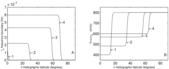
Figure 2: Panel A: Sketch of the latitudinal distribution of the lower boundary of the frequency spectrum. The curves correspond to four different phases of the solar cycle: $t^{\prime}=0,1.5,3.5$ and $5.5$ (years counted from minimum activity) labeled 1 to 4, respectively. Panel B: Sketch of the observed distribution of the total speed $V$ vs. latitude. The four curves are shown in the same order as in Panel A.

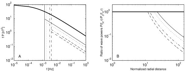
Figure 3: The linestyles correspond to four different stages of the solar cycle in the following order: $t^{\prime}=0$ (thin solid line), $t^{\prime}=1.5$ (dotted line), $t^{\prime}=3.5$ (dashed-dotted line) and $t^{\prime}=5.5$ (dashed line). Panel A: The scaled wave power spectra ($fP$) vs. frequency at 0.3 AU. The thick solid line is the complete spectrum of the reference model. The vertical lines mark the cut-off frequencies $f_{0}$ at four different stages of the solar cycle. Panel B: Ratio of the spectral powers, at the corresponding dissipation frequencies, calculated using the considered frequency domain truncation and the one taken from the reference model: The difference between the reference values (thick horizontal line ) and the updated turbulence spectra (the curves) is a result of their low-frequency truncation within the inertial range.

5 Quantitative analysis and proof of the concept’s validity

We aim to perform an appropriate quantitative study of the problem in order to obtain a consistent proof of the proposed concept. As we study the possibility of the presence of lower frequency cut-offs in the Alfvén wave spectra above streamer-like structures, it is natural to assume that the locations of such restricted sources are linked with the latitudinal extent of the streamer generating zone and its variation with the solar cycle.

In this paper we show how the frequency cut-off affects the wave spectrum as well as the heating and acceleration rates. Therefore, like in Vainio et al. (2003), we use $V=400$ km s^-1 as a target velocity. Using this value we derive four characteristic values of the cut-off frequencies: 1) $f_{0}=10^{-6}$ Hz. This is the case recovering the one in reference model (case of no truncation) as in this case the cut-off frequency remains outside the inertial range along the entire domain of computation so that there is no modification of the spectrum. 2) the other valuas are calculated and shown in Panel A of Fig. 3 as vertical lines at $f_{0}=1.3\cdot 10^{-3}$ Hz. (solar minimum, $t^{\prime}=0$ (solid line), $f_{0}=1.8\cdot 10^{-3}$ Hz ($t^{\prime}=1.5$ (dotted line)), $f_{0}=3.0\cdot 10^{-3}$ Hz. ($t^{\prime}=3.5$ (dashed-dotted line)) and $f_{0}=4.0\cdot 10^{-3}$ Hz. (solar maximum, $t^{\prime}=5.5$ (dashed line))). In the same panel we plot the spectra at 0.3 AU corresponding to these five cases. In panel B of Fig. 3 we plot the ratio of the spectral powers calculated using the considered frequency domain truncation and the one taken from the reference model. The points of break at which the curves corresponding to the updated spectra start to deviate from the reference values (the thick horizontal line) mart the distances at which $\tau=1$ ($f_{c}=f_{0}$). These curves were obtained using updated spectra acurately calculated in this paper and given by expression (26) (case $q=1$). In Vainio et al. (2003) it has been shown that there is only a small difference between convective and diffusive formulations of the flux function $F$. We concentrate on the first approach and consequently use:

$$F=2\pi C^{2}\frac{v_{A}}{V}\frac{f^{5/2}P^{3/2}}{B}.$$ (31)

The physical quantities in the latter expression are defined as follows:

$$P\left(f,r\right)\approx\left\{\begin{array}[c]{ll}\frac{P_{\rm{WKB}}(f,r)}{1+\left[f/f_{c}(r)\right]^{2/3}}&\text{if }f_{0}\leq f_{c}\\ \frac{P_{\rm{WKB}}(f,r)}{1+\left[f_{0}/f_{c}(r)\right]^{2}\left[f/f_{0}\right]^{5/3}}&\text{if }f_{0}>f_{c}\end{array}\right.$$ (32)

with

$$P_{\rm{WKB}}(f,r)=P(f,r_{\sun})\frac{B(r)v_{A}(r)}{B_{\sun}v_{A\sun}},$$ (33)

representing the part of the spectral power outside the inertial range where waves follow predominantly a WKB behaviour and where

$$P(f,r_{\sun})=\varepsilon_{P}\frac{B_{\sun}^{2}}{f}H\left(1-\left(\frac{f_{0}}{f}\right)^{\frac{2}{3}}\right),$$ (34)

and $f_{c}(r)$ is the breakpoint frequency at which the Kolmogorov type of the spectrum starts to prevail:

$$\frac{1}{f_{c}(r)}=2\pi\varepsilon_{P}^{1/2}\int_{r_{\sun}}^{r}\frac{C^{2}(r^{\prime})v_{A}(r^{\prime})}{V^{2}}\left(\frac{n_{e\sun}}{n_{e}(r^{\prime})}\right)^{1/4}dr^{\prime}.$$ (35)

Here $\varepsilon_{P}$ is a dimensionless spectral parameter determining the intensity of wave excitation. Its value in the case of absence of additional wave sources is set to $5\cdot 10^{-5}$. In general, a more complete model of the solar wind must include also angular components of velocities, however for the sake of simplicity we assume those components to be vanishing. $C^{2}(r)=\alpha\alpha_{1}(r)$ is a model parameter, where $\alpha$ is a cascading constant and

$$\alpha_{1}=\left\{\begin{array}[]{l l}\alpha_{0}\left(\frac{r-r_{\sun}}{9r_{\sun}}\right)&\hskip 5.69046ptr_{\sun}\leq r<10r_{\sun}\\ \alpha_{0}&\hskip 5.69046ptr\geq 10r_{\sun}\\ \end{array}\right.,$$ (36)

with $\alpha_{0}$ another dimensionless parameter determining the ratio of outward and inward propagating wave intensities. Its value when additional sources are absent is set to 0.05.

We have also performed computations for the solar wind acceleration due to the wave pressure gradient ${\vec{\nabla}}p_{w}$. As in Vainio et al. (2003), we use explicit the expression:

$$p_{w}=\frac{v_{A}}{v_{A\sun}}\frac{A_{\sun}}{A}p_{w\sun}-\frac{v_{A}}{2VA}\int_{r_{\sun}}^{r}\frac{A(r^{\prime})}{v_{A}(r^{\prime})}Q(r^{\prime})dr^{\prime},$$ (37)

where $A\propto 1/B$ is a cross sectional area of the open field structure. The results of calculations are shown in Fig. 4 Panel B. Again, the thick solid curve shows the radial distribution of the wave pressure gradient $-(m_{p}n_{e})^{-1}\partial p_{w0}/\partial r$ corresponding to the case of no cut-off and, thus, the reference model. The calculations for $-(m_{p}n_{e})^{-1}\partial p_{w}/\partial r$ are done for the above-mentioned four epochs of the solar cycle shown by the thin curves with the same order of the linestyles as in Panel A. It is seen that the acceleration rate decreases significantly (according to these calculation by 15-25 percent) within the first ten solar radii from the solar surface, while it monotonically decreases in absolute value beyond this distance. To summarise this part of our investigation we conclude that the truncation of the available wave spectrum from the lower frequency side leads to a significant decrease in both heating and acceleration rates and, therefore, this proves the main message of this paper that the effect of the lower frequency boundary $f_{0}$ should not be abandoned in the slow wind models.

The analysis above lets us conclude that if only one kind of wave sources would operate in the equatorial zone then the appearance of more and more streamer-like open structures with increasing solar activity – leading to a gradual decrease of their transversal spatial scales – would result in significant cooling of the wind plasma above the distance of 10 solar radii and deceleration of the wind stream even within that zone (what is actually observed outside the sunspot generating zone at high latitudes (Richardson et al., 2001)). However, observations evidence (Kasper et al., 2007) that there clearly operate two kinds of wave sources with relative significance at different stages of the solar cycle. It is reasonable to assume that these growing number of small-scale magnetic structures in the vicinity of active zones increases the probability of reconnections, on the one hand, and leads to creation of additional small-scale open field structures anchored in active zones, on the other hand. It is conventionally presumed that those reconnection processes shake these open structures and, thus, represent so-called active region sources of additional wave power. A significant number of such small structures has a reasonable potential to compensate the losses of energy arising from the truncation of the lower frequency part of the spectrum. In other words, even though for low frequency modes the equatorial part of the atmosphere is not accessible, increased wave power is nevertheless available in the high-frequency part of the spectrum above the cut-off frequencies $f_{0}$. One could ask here: what should be an actual value of the higher frequency wave power to compensate the losses in thermal and mechanical energy production rates obtained above? As we mentioned above this issue stays outside the scope of the current study. It should be noted that observed wave spectra (e.g. see in Tu & Marsch, 1996) contain a combined wave power supplied by the sources from entire coronal holes (including polar regions) and some possible local sources not located on the Sun, but in the solar wind. This is why, possibly, the truncation of the power spectra as shown in Figure 3 is not observationally resolvable so far. However, large error bars in the spectra below the frequencies 10^-2 Hz maybe the indication that the significant decline in the wave power for low frequencies could be observable with higher spectral resolution.

6 Discussion and conclusions

As is conventionally accepted, the physical grounds underlying the appearance of the fast and slow winds are substantially different. The fast wind originates in the unipolar magnetic configurations of coronal holes with open field line topology, while most of the indirect measurements of the active region evolution during the solar cycle, like detections of the helium abundance in the solar wind, indicate that multiple processes for slow wind heating and acceleration should operate in the different proportions at different phases of the solar cycle (Kasper et al., 2007). There is the process related to the heliographic current sheet and the streamer belt (Einaudi et al., 2000, 2001), which at the equatorial region is most active at solar minimum (Kasper et al., 2007). With the uptrend of the activity cycle the significance of the streamer belt contribution decreases gradually reaching some smaller but finite rates at maximum. At the same time more and more streamer-like structures appear at high latitudes covering practically the entire solar disk at maximum activity with relatively small-scale structures. These structures lead to the cut-off frequencies of the wave spectra generated within those streamers resulting in reduced acceleration and heating of the plasma outflow. This scenario is in good agreement with the observations at high latitudes.

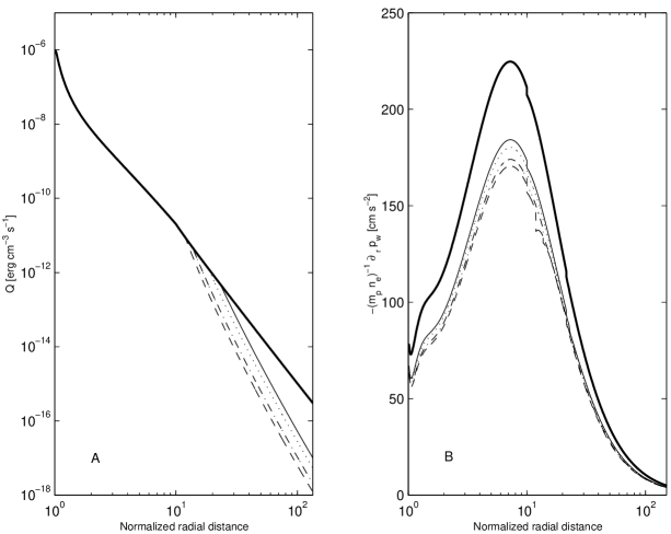
Figure 4: Panel A: Calculated heating rates $Q_{0}$ (reference model, thick solid line), $Q$ (modified heating using the four truncated spectra shown in Fig. 3. Panel B: Calculated wave pressure gradients for the reference model $-(m_{p}n_{e})^{-1}\left(\partial p_{w0}/\partial r\right)$ (thick solid line) and for the truncated spectra $-(m_{p}n_{e})^{-1}\left(\partial p_{w}/\partial r\right)$. The linestyles correspond to Panel A.

A detailed numerical validation of the presented paradigm of the wave spectra formation is beyond the primary scope of the current paper where we focus on the physical grounds of the underlying the concept. While more extended numerical studies via direct simulations will be published elsewhere, here we demonstrate in general terms a correspondence of the above-stated scenario with the existing data and modern understanding of the solar wind acceleration scenarios.

At the solar minimum the sources located in the current sheet and streamer belt dominate and the dynamics of the process is governed by the ambient low frequency Alfvén waves (Einaudi et al., 2001) for which the equatorial region is accessible to some extent because of the more regular spatial structure of the magnetic field below the cusp. The structure of the magnetic field resembles a dipole field at that stage. With the change of the magnetic field topology the streamer zone spreads to very high latitudes and, at the same time, new open field lines appear which are anchored in the active regions and are fed from the latter with the modified spectrum of Alfvén wave disturbances (Liewer et al., 2004; Kasper et al., 2007). Therefore, the excited wave spectrum, following the spatial scales of the modified sources, becomes truncated from the low frequency side. Besides, with the increasing number of these new active magnetic structures, the rate of confinement of the plasma at low heliospheric distances leading to a significant modification of the density profile may also grow.

In fact, the scenario developed in this paper is an attempt to formulate a mathematical scheme for a modeling of the slow solar wind throughout the entire latitudinal domain and throughout the solar activity cycle. Of course, our considerations are based on substantial assumptions regarding the fine structure of temporal and latitudinal variation of physical quantities. More rigorous astrophysical modeling is needed to explore further specifics of the Alfvén wave frequency domain in the solar atmosphere that should comprise, e.g., the north-south asymmetry of the sunspot distribution, deviation from normal latitudinal distributions, or non-equilibrium components of the observed statistics. The results can have far reaching impact on the understanding of the solar and, in general, stellar wind origin. This aspect is also of interest in the stellar wind context in connection with the currently emerging field of stellar wind dynamics and interaction with extrasolar planets.

References

- Bamert et al. (2008) Bamert, K., Kallenbach, R., le Roux, J. A., Hilchenbach, M., Smith, C. W., and Wurz, P., (2008), ApJ, 675, L45
- Chen et al. (2010) Chen, C. H. K., Horbury, T. S., Schekochihin, A. A., Wicks, R. T., Alexandrova, O., and Mitchell, J., (2010), Phys. Rev. Lett. 104, 255002
- Cirtain et al. (2007) Cirtain J. W. et al., (2007), Science, 318, 1580
- dePontieu et al. (2007) De Pontieu, B. et al., (2007), Science, 318, 1574
- Einaudi et al. (2000) Einaudi G., Boncinelli, P., Dahlburg, R. B., and Karpen, J. T., Advances in Space Research, (2000), 25, 1931
- Einaudi et al. (2001) Einaudi, G., Chibbaro, S., Dahlburg, R. B., and Velli, M., (2001), ApJ, 547, 1167
- Elfimov et al. (2004) Elfimov, A. G., Galvão, R. M. O., Jatenco-Pereiredra, V., and Opher, R., (2004), ApJ, 600, 292
- van der Holst et al. (2007) van der Holst, B., Jacobs, C., and Poedts, S., (2007), ApJ 671, L77
- Hu et al. (1999) Hu, Y. Q., Habbal, S. R., and Li, X., (1999), J. Geophys. Res., 104, 24819
- Kasper et al. (2008) Kasper, J. C., Lazarus, A. J., and Gary, S. P., (2008), Phys. Rev. Lett. 101, 261103
- Kasper et al. (2007) Kasper, J. C., Stevens, M. L., Lazarus, A. J., Steinberg, J. T., and Ogilvie, K. W., (2007), ApJ, 660, 901
- Kleimann et al. (2009) Kleimann, J., Kopp, A., Fichtner, H., and Grauer, R., (2009), Annales Geophysicae, 27, 989
- Liewer et al. (2004) Liewer, P. C., Neugebauer, M., and Zurbuchen, T., (2004), Solar Phys., 223, 209
- Luo & Wu (2010) Luo, Q. Y. and Wu, D. J., (2010), ApJ, 714, L138
- Marino et al. (2008) Marino, R., Sorriso-Valvo, L., Carbone, V., Noullez, A., Bruno, R., and Bavassano, B., (2008), ApJ 677, L71
- Narain & Agarwal (1994) Narain, U. and Agarwal, P., (1994), Bulletin of the Astronomical Society of India, 22, 111
- Oughton & Matthaeus (2005) Oughton, S., and Matthaeus, W. H., (2005), Nonlin. Processes Geophys., 12, 299
- Richardson et al. (2001) Richardson, J. D., Wang C., and Paularena, K.I., (2001), Adv. Space. Res, 27, 471
- Sahraoui et al. (2009) Sahraoui, F., Goldstein, M. L., Robert, P., and Khotyaintsev, Y. V., (2009), Phys. Rev. Lett. 102, 231102 .
- Shergelashvili et al. (2006) Shergelashvili, B. M., Poedts, S., and Pataraya, A. D., (2006), ApJ, 642, L73
- Tu et al. (1984) Tu, C., Pu, Z., and Wei, F., (1984), J. Geophys. Res. 89, 9695 .
- Tu & Marsch (1996) Tu, C. and Marsch, E., (1996), Space Sci. Rev. 77, 372
- Ulmschneider et al. (2001) Ulmschneider, P., Fawzy, D., Musielak, Z. E., and Stepień, K., (2001), ApJ 559, L167
- Vainio et al. (2003) Vainio, R., Laitinen, T., and Fichtner, H., (2003), A&A 407, 713