Driving Markov chain Monte Carlo with a dependent random stream

Abstract

Markov chain Monte Carlo is a widely-used technique for generating a dependent sequence of samples from complex distributions. Conventionally, these methods require a source of independent random variates. Most implementations use pseudo-random numbers instead because generating true independent variates with a physical system is not straightforward. In this paper we show how to modify some commonly used Markov chains to use a dependent stream of random numbers in place of independent uniform variates. The resulting Markov chains have the correct invariant distribution without requiring detailed knowledge of the stream’s dependencies or even its marginal distribution. As a side-effect, sometimes far fewer random numbers are required to obtain accurate results.

1 Introduction

Markov chain Monte Carlo (MCMC) is a long-established, widely-used method for drawing samples from complex distributions (e.g., Neal, 1993). Simulating a Markov chain yields a sequence of states that can be used as dependent samples from a target distribution of interest. If the initial state of the chain is drawn from the target distribution, the marginal distribution of every state in the chain will be equal to the target distribution. It is usually not possible to draw a sample directly from the target distribution. In that case the chain can be initialized arbitrarily, and the marginal distributions of the states will converge to the target distribution as the simulation progresses. The states of the chain are often used to approximate expectations, such as those required by stochastic approximation optimization algorithms, or Bayesian inference. Estimating expectations does not require independent samples, and any bias from an arbitrary initialization disappears in the limit of long Markov chain simulations. Bias can also be reduced by discarding all samples collected during an initial ‘burn-in’ period, and estimating an expectation using only the samples collected after a certain point in the chain.

Usually Markov chains are simulated with deterministic computer code that makes choices based on an independent stream of random variates, often drawn from $\mathrm{Uniform}[0,1]$. In practice, most implementations use pseudo-random numbers as a proxy for ‘real’ random numbers. Noisy physical systems can potentially be used to provide ‘real’ random numbers, although these are slow when used rigorously (see section 2). Early hardware implementations of stochastic neural networks had problems with dependencies in their noise sources (Alspector et al., 1989). Back then, hope and empirical performance (rather than theory) were used to justify using dependent random numbers.

Taking a standard MCMC code and replacing its independent variates with dependent variates will usually lead to biases. As a simple tractable example, consider the Gaussian random walk

$$x_{t+1}\;\leftarrow\;\alpha x_{t}+\sqrt{1-\alpha^{2}}\;\nu_{t},\qquad\nu_{t}\sim\mathcal{N}(0,1),$$ (1)

where $0\!<\!\alpha\!<\!1$. This chain will explore a unit Gaussian distribution: $x_{t}$ will be distributed as $\mathcal{N}(0,1)$, either in the limit $t\!\rightarrow\!\infty$, or for all $t$ if $x_{1}$ was drawn from $\mathcal{N}(0,1)$. If the noise terms were dependent in some way, then the variance of the equilibrium distribution could be altered. For example, if the random variates at even time-steps were a copy of the variate at the previous time step (i.e., $\nu_{2}\!=\!\nu_{1}$, $\nu_{4}\!=\!\nu_{3}$, …) then the equilibrium variance would increase from 1 to $(1+\alpha)^{2}/(1+\alpha^{2})$. In most MCMC algorithms the random variates driving the Markov chain — $\nu$ in this example — must be independent and come from a specified marginal distribution.

Given that the output of an MCMC algorithm is a dependent sequence, it is not clear that the variates used to drive the chain must necessarily be independent. In this paper we give a constructive demonstration that it is possible to modify many standard MCMC codes so that they can be driven by a dependent random sequence. Surprisingly, our construction does not depend on the functional form of the dependencies, or on the marginal distribution of the dependent stream.

2 Random number generation in practice

Recent papers using MCMC methods rarely discuss or specify the underlying random number generator used to perform Markov chain simulations. A common view is that many pseudo-random number generators are good enough for many purposes, but only some of the slower more complex generators are completely trusted. For example, Skilling (personal communication) reports his experience on using one of the generators from Numerical Recipes (Press et al., 2002) within BayeSys (Skilling, 2004):

“Although I used this procedure heavily for more than ten years without noticing any damage, one recent test gave weakly but reproducibly biased results. This bias vanished on replacing the generator, so I have discarded ran3 despite its speed.”

Similarly there are known problems with the default, although fast, random number generator provided by Matlab (Savicky, 2006). Switching to more modern generators is easy to do, and it is widely thought that the state-of-the-art pseudo-random number generators are good enough for most Monte Carlo purposes. Nevertheless, it is hard to be certain there will not be problems with using pseudo-random numbers in a given application.

The “Flexible Bayesian Modelling” (FBM) software by Neal (2004) calls a standard Unix pseudo-random number generator known as drand48. Although this pseudo-random number generator performs reasonably, it has known problems in some circumstances (Entacher, 1998), which (in a seemingly isolated incident) have lead to errors in an application (Gärtner, 2000). Although FBM would probably have no practical problems using drand48 only, the code is somewhat robust to possible difficulties by also making use of a file of 100,000 ‘real’ random numbers.

Combining numbers from a physical source and a pseudo-random generator is also common in cryptography. For example the Intel generator works in this way (Jun and Kocher, 1999). However, most of the development of these methods has been focussed on ensuring that the random bits are unpredictable enough to prevent encryption schemes from being cracked, and also that the discovery of the internal state of the generator does not allow the bits to be easily reconstructed. The Intel team were careful to be quite guarded about the quality of the random numbers from their hardware. Some deviations from independent uniform randomness are possible, but no analysis of the resulting potential bias in Monte Carlo work has been reported.

From a computer science theory perspective, obtaining independent random bits from a random source is known as ‘randomness extraction’ (e.g., Shaltiel, 2002), and can come with a variety of guarantees. In practice, generating independent uniform random numbers from a physical source is tricky and slow. See the HotBits online service (http://www.fourmilab.ch/hotbits/) for an example of what can be involved. The Linux random number generators (/dev/random and /dev/urandom) operate by gleaning entropy from system events. But their entropy pool can be exhausted quickly (Gutterman et al., 2006).

Random number generating hardware could potentially be made simpler and faster if the requirement for independent uniform variates were removed. We will show that it is indeed possible to adapt Markov chain Monte Carlo to use any source of random numbers, and that far less randomness may be required than is commonly used.

3 Markov chain Monte Carlo, setup and preliminaries

A Markov chain transition operator $T(x^{\prime}\!\leftarrow\!x)$ specifies a probability distribution over the next state $x^{\prime}$ given the current state $x$. If the Markov chain is defined over a finite set of states, then $T(x^{\prime}\!\leftarrow\!x)$ is a probability mass function over $x^{\prime}$ for every fixed $x$. Otherwise, if the states are continuous, then $T(x^{\prime}\!\leftarrow\!x)$ is a probability density. Given a target distribution $\pi(x)$, standard MCMC techniques require a transition operator that leaves the target invariant:

$$\pi(x^{\prime})=\sum_{x}T(x^{\prime}\!\leftarrow\!x)\,\pi(x)\qquad\text{or}\qquad\pi(x^{\prime})=\int T(x^{\prime}\!\leftarrow\!x)\,\pi(x)\;\mathrm{d}{x}.$$ (2)

The Markov chain produced by the operator should also be ergodic, meaning that any starting state should eventually be ‘forgotten’ and the marginal distribution of the chain should converge to the target distribution, $\pi(x)$. Such ergodic chains have the target distribution as their equilibrium distribution. A simple sufficient condition for ergodicity in the discrete setting is that there is a non-zero probability of transitioning from any state to any other state in $K$ transitions for some finite $K$ (e.g., Neal, 1993). Some care is required for defining ergodicity in the continuous setting. The technical details, and more formal definitions of the above, are outlined by Tierney (1994).

A transition operator that leaves the target distribution invariant (one that satisfies equation 2) can be created by concatenating together several operators that each satisfy (2) individually. The component operators do not need to be ergodic in isolation. To build an MCMC method, first one finds a useful set of operators that each satisfy (2), and second, one checks ergodicity for the composition of the operators (e.g., Tierney, 1994).

For any transition operator satisfying (2), one can define a reverse operator:

$$\widetilde{T}(x\!\leftarrow\!x^{\prime})=\frac{T(x^{\prime}\!\leftarrow\!x)\,\pi(x)}{\int T(x^{\prime}\!\leftarrow\!x)\,\pi(x)\;\mathrm{d}{x}}=\frac{T(x^{\prime}\!\leftarrow\!x)\,\pi(x)}{\pi(x^{\prime})}\,.$$ (3)

The existence of such a reverse operator is a necessary condition for any operator that leaves the target distribution invariant. This condition is also sufficient: if the reverse operator exists, then we can form a symmetric version of (3),

$$\widetilde{T}(x\!\leftarrow\!x^{\prime})\,\pi(x^{\prime})=T(x^{\prime}\!\leftarrow\!x)\,\pi(x),$$ (4)

which, integrated or summed over $x$ on both sides, implies (2). If an operator is reversible, $T\!=\!\widetilde{T}$, the condition is known as detailed balance.

In many MCMC algorithms involving distributions on random vectors, the coordinates of the vector are updated sequentially by component operators of the algorithm. For such algorithms, we need only consider operators that act on one-dimensional random variables. Suppose $T$ is a component operator of an MCMC algorithm. Often $T$ is implemented as a deterministic function of a uniform variate $u$, $x^{\prime}\!=\!\tau(u;x)$. In this case, the Markov chain can be driven using a sequence of uniform random variates $u_{1},u_{2},\ldots$, by initializing the chain at $x_{1}$ and computing $x_{2}\!=\!\tau(u_{1};x_{1}),x_{3}\!=\!\tau(u_{2},x_{2}),\ldots$.

For a transition operator that acts on a continuous random variable, we can take $\tau$ to be the inverse cumulative distribution function (cdf) of the transition operator:

$$\tau^{-1}(x^{\prime};x)=\int_{-\infty}^{x^{\prime}}T(\hat{x}\!\leftarrow\!x)\;\mathrm{d}\hat{x}.$$ (5)

Evaluating the inverse cdf, $\tau(\,\cdot\,;x)$, at a uniform variate $u$ produces a sample from the transition operator. If an independent uniform variate $u$ is drawn for each update, then the Markov chain will have the desired equilibrium distribution.

For discrete variables

$$\tau(u;x)=\min\left\{x^{\prime}:u>\sum_{\hat{x}<x^{\prime}}T(\hat{x}\!\leftarrow\!x)\right\},$$ (6)

is the analogous deterministic function. We can implement the reverse transition operator as a deterministic function of a uniform variate by setting $x\!=\!\tilde{\tau}(u;x^{\prime})$ where

$$\tilde{\tau}^{-1}(x;x^{\prime})=\int_{-\infty}^{x}\widetilde{T}(\hat{x}\!\leftarrow\!x^{\prime})\;\mathrm{d}\hat{x}.$$ (7)

The reverse move for discrete variables is defined analogously.

4 Constructing a Markov chain from a dependent stream

We now assume that we do not have access to independent random variates with which to drive the chain. Instead, we have access to a stream of random variates, $d_{t}$, with arbitrary dependencies. We will find that it is possible to construct valid Markov chain Monte Carlo algorithms — chains with the correct invariant distribution — without knowing any details of the dependency structure of the stream, or even the marginal distribution of its output. The speed with which the chain reaches equilibrium will depend on properties of the stream. Proving ergodicity will require some additional, but weak, conditions.

We wish to adapt existing MCMC algorithms to use dependent streams. We initially restrict attention to operators driven by a single uniform random variate, as outlined in section 3. Given that we do not have an external source of uniform variates, we will include one in our state; we will run a Markov chain on a pair $(x,u)$ with target distribution

$$\pi_{a}(x,u)=\begin{cases}\pi(x)&\text{if~{}~{}$0<u<1$}\\ 0&\text{otherwise.}\\ \end{cases}$$ (8)

To obtain samples from the target distribution we can simulate a Markov chain that has equilibrium distribution (8), and discard the auxiliary $u$ samples. Our Markov chain Monte Carlo algorithm will concatenate transition operators that each leave the joint auxiliary distribution invariant.

4.1 Operator 1

We define an operator that adds the current stream output, $d_{t}$, to the uniform variate with a wraparound at one:

$$u_{t+1}=(u_{t}+d_{t})\,~{}\mathrm{mod}~{}1.$$ (9)

By $u\;\mathrm{mod}\;1$ we mean $u\!-\!\lfloor u\rfloor$ (e.g., $9.1\,~{}\mathrm{mod}~{}1=0.1$  and  $-8.3\,~{}\mathrm{mod}~{}1=0.7$). This operation leaves the target uniform distribution invariant: the marginal distribution of the sum modulo one of any real number and a uniform draw is $\mathrm{Uniform}[0,1]$.

4.2 Operator 2

Given a sample $(x,u)$ from the auxiliary distribution 8, we could obtain another dependent sample from the target distribution, $\pi(x)$, by using the uniform variate to take a Markov chain step:

$$x^{\prime}=\tau(u;x).$$ (10)

The function $\tau$ is the inverse of the cumulative distribution function (5) for the transition operator of the MCMC algorithm that we are adapting. To create an update that leaves the joint auxiliary distribution invariant we must also modify the uniform variate such that a reverse procedure exists that will map $(x^{\prime},u^{\prime})\!\rightarrow\!(x,u)$. Such a reverse procedure must exist if we wish to satisfy the balance condition (4) for the joint auxiliary distribution.

For continuous variables we simply set the uniform variate to the value that would drive the reverse transition operator to move from ${x^{\prime}\!\rightarrow\!x}$:

$$u^{\prime}=\int_{-\infty}^{x}\widetilde{T}(\hat{x}\!\leftarrow\!x^{\prime})\;\mathrm{d}\hat{x}.$$ (11)

The new $(x^{\prime},u^{\prime})$ pair is the result of the two changes of variable in equations (10) and (11). Therefore, the joint distribution of $(x^{\prime},u^{\prime})$ can be found by multiplying $\pi_{a}(x,u)$ by the Jacobian of the change of variables:

$$P(x^{\prime},u^{\prime}) =\pi_{a}(x,u)\cdot\left|\frac{\partial u}{\partial x^{\prime}}\right|\cdot\left|\frac{\partial x}{\partial u^{\prime}}\right|$$ (12)

$$=\pi(x)\cdot T(x^{\prime}\!\leftarrow\!x)\cdot 1/\widetilde{T}(x\!\leftarrow\!x^{\prime})$$ (13)

$$=\pi(x^{\prime}).$$ (14)

We substituted (3) and (8), assuming that the initial state is feasible (i.e., that $u\in[0,1]$). By construction, $u^{\prime}\in[0,1]$ and so the probability of the final pair is given by the target distribution, $\pi_{a}(x^{\prime},u^{\prime})$. Thus $\pi_{a}$, the target distribution (8), is invariant under this operator.

For discrete variables there are a range of uniform values, $u\in[u_{\mathrm{min}},u_{\mathrm{max}}]$, that yield the same forwards move $x^{\prime}\!=\!\tau(u;x)$. Similarly a reverse move, $x\!=\!\tilde{\tau}(u^{\prime};x^{\prime})$, defined with the reverse transition operator could be made using any value in the range $u^{\prime}\in[u^{\prime}_{\mathrm{min}},u^{\prime}_{\mathrm{max}}]$. The ranges are given by:

$$u_{\mathrm{min}} =\sum_{\hat{x}<x^{\prime}}T(\hat{x}\!\leftarrow\!x) u^{\prime}_{\mathrm{min}} =\sum_{\hat{x}<x}\widetilde{T}(\hat{x}\!\leftarrow\!x^{\prime})$$

$$u_{\mathrm{max}} =u_{\mathrm{min}}+T(x^{\prime}\!\leftarrow\!x) u^{\prime}_{\mathrm{max}} =u^{\prime}_{\mathrm{min}}+\widetilde{T}(x\!\leftarrow\!x^{\prime}).$$ (15)

We need a procedure that picks a new uniform variate $u^{\prime}$ in a way that could be reversed to recover the original variate $u$. We choose the procedure that leaves the fraction through the available ranges constant:

$$u^{\prime} =u^{\prime}_{\mathrm{min}}+(u^{\prime}_{\mathrm{max}}-u^{\prime}_{\mathrm{min}})\frac{u-u_{\mathrm{min}}}{u_{\mathrm{max}}-u_{\mathrm{min}}}$$ (16)

$$=\sum_{\hat{x}<x}\widetilde{T}(\hat{x}\!\leftarrow\!x^{\prime})+\frac{\widetilde{T}(x\!\leftarrow\!x^{\prime})}{T(x^{\prime}\!\leftarrow\!x)}\bigg{(}u-\sum_{\hat{x}<x^{\prime}}T(\hat{x}\!\leftarrow\!x)\bigg{)}.$$ (17)

In the discrete setting, the probability of the state update (10) is one. The probability of obtaining a new joint state, deterministically transformed from an equilibrium state, is:

$$P(x^{\prime},u^{\prime})=\pi(x,u)\cdot 1\cdot\left|\frac{\partial u}{\partial u^{\prime}}\right|=\pi(x)\frac{T(x^{\prime}\!\leftarrow\!x)}{\widetilde{T}(x\!\leftarrow\!x^{\prime})}=\pi(x^{\prime}).$$ (18)

Again the update leaves the joint auxiliary distribution invariant.

4.3 The algorithm and its properties

Applying Operators 1 and 2 alternately in sequence will leave the joint auxiliary distribution invariant. If the transition operator of the MCMC algorithm that we are adapting is formed by a composition of transition operators, then the underlying transition distribution $T$ used in Operator 2 should cycle through each component of the composition. The algorithm is presented in Fig. 1.

Although the sequence resulting from this algorithm will always leave the auxiliary distribution invariant, it will only be ergodic if the random stream satisfies some conditions. For example, if the stream were to always emit a zero, then Operator 1 will have no effect. In this case, if $T$ were given by a single reversible component, then the sequence would alternate between $x_{1}$ and $\tau(0,x_{1})$ and would thus not be ergodic. At the other extreme, if the stream is actually an independent source of $\mathrm{Uniform}[0,1]$ random variates, then $u^{\prime}\!=\!\left(u+d\right)\,\mathrm{mod}~{}1$ is also a uniform variate that is independent of the current Markov chain state $(u,x)$. In this case, the statistics of the original Markov chain are recovered exactly.

If the original transition operator that we are modifying is ergodic, it will have sets $X^{\prime}$ that can be reached with positive probability from any given state $x$ in a finite number of steps. The transitions to a set $X^{\prime}$ can be realized by a set of sequences of driving random numbers. If every sequence of stream outputs can be realized (i.e., if the density of $d_{t}$ dominates the Uniform$[0,1]$ distribution for every possible stream history), then our method will have the same reachable sets. Thus, the proofs of ergodicity for most algorithms will be maintained. Our method may also produce ergodic chains for some more constrained dependent streams, although a proof would depend on the MCMC algorithm being modified.

If ideal independent random numbers are available, but are slow to obtain, these could be used for a small fraction of iterations and a pseudo-random stream used for the remaining iterations. The resulting chain will leave the target distribution invariant, and under weak conditions it will also be ergodic. For example, the usual proofs of ergodicity rely on sets of states that have positive probability measure after $K$ transition steps, regardless of starting position, for some finite $K$. These sets are still accessible if we regularly perform $K$ of the original transitions, using independent Uniform$[0,1]$ numbers. In between these sequences of updates we can interleave long runs of transitions driven by the dependent stream. These intermediate runs might each be constrained to some partition of the space, but the combined chain can potentially get anywhere and will still converge. In contrast, ad-hoc schemes for combining poor-quality random numbers with an ideal physical source provide no such guarantees.

Inputs: Initial augmented state $(x,u)$; dependent stream $\mathcal{D}$; operators $\{T_{n}(x^{\prime}\!\leftarrow\!x)\}_{n=1}^{N}$,

Inputs: with inverse cumulatives $\tau_{n}(u;x)$ and reverse operators $\{\widetilde{T}_{n}(x^{\prime}\!\leftarrow\!x)\}$ (see (3))

1. for $n=1\dots N$: Operator 1: 2. Query the stream: $d\sim\mathcal{D}$ 3. $u\leftarrow\left(u+d\right)\,\mathrm{mod}~{}1$   — introduces randomness, replaces $u\sim\mathrm{Uniform}[0,1]$ Operator 2: 4. $x_{\mathrm{old}}\leftarrow x$ 5. $x\leftarrow\tau_{n}(u;x)$      — as in conventional update with random uniform $u$ 6. if $x$ is discrete: 7. $u\leftarrow\sum_{\hat{x}<x_{\mathrm{old}}}\widetilde{T}(\hat{x}\!\leftarrow\!x)+\frac{\widetilde{T}(x_{\mathrm{old}}\,\!\leftarrow\!\,x)}{T(x\,\!\leftarrow\!\,x_{\mathrm{old}})}\Big{(}u-\sum_{\hat{x}<x}T(\hat{x}\!\leftarrow\!x_{\mathrm{old}})\Big{)}$ (17) 8. else: 9. $u\leftarrow\int_{-\infty}^{x_{\mathrm{old}}}\widetilde{T}_{n}(\hat{x}\!\leftarrow\!x)\;\mathrm{d}\hat{x}.$ (5)

Figure 1: Procedure for applying a set of simple conventional Markov chain transition operators while using a dependent stream. Section 5 discusses applicability to less-tractable transition operators.

5 Application to common MCMC algorithms

Not all commonly-used MCMC procedures have transition operators that use a single driving random number $u$, and that are tractable enough to apply the method described in the previous section. However, if a method can be implemented in practice, it can usually be broken down into a series of deterministic operations driven by a set of uniform variates. Also, a corresponding reverse operator will have been identified to prove that the necessary balance condition (4) holds. These observations allow us to generalize our procedure (Fig. 1) to other algorithms.

Our strategy for adapting existing Markov chain Monte Carlo algorithms to use a dependent stream will be as follows: 1) include the required random numbers in the state; 2) update uniform variates by addition module-one with the stream; 3) apply deterministic moves that change the variables of interest using the uniform variates, and update the uniform variates so that the move would be reversed under the reverse operator. We now give some details of applying this strategy to some of the most commonly-used MCMC algorithms.

5.1 Gibbs Sampling

Gibbs sampling is one of the most commonly used MCMC methods for sampling a set of variables $x\!=\![x_{1},\dots,x_{N}]$. Each variable is resampled in turn from its conditional distribution. For continuous variables:

$$T_{n}(x^{\prime}\!\leftarrow\!x)=\pi(x^{\prime}_{n}\!\mid\!x_{m\neq n})\,\delta(x^{\prime}_{m\neq n}-x_{m\neq n}),$$ (19)

and for discrete:

$$T_{n}(x^{\prime}\!\leftarrow\!x)=\begin{cases}\pi(x^{\prime}_{n}\!\mid\!x_{m\neq n})&x^{\prime}_{m\neq n}=x_{m\neq n}\\ 0&\text{otherwise.}\end{cases}$$ (20)

Provided these conditional distributions are sufficiently tractable, the algorithm in Fig. 1 applies directly. Example code is provided as supplementary material.

Gibbs sampling is also performed on distributions without tractable conditional distributions. The techniques for sampling from these distributions often require a random number of independent uniform variates (e.g., Gilks and Wild, 1992; Gilks, 1992; Devroye, 1986). An example application to a method with this flavor is given in Section 5.3.

5.2 Metropolis–Hastings

In the Metropolis–Hastings transition rule (Hastings, 1970), a sample is drawn from an arbitrary proposal density $q(x^{\prime};x)$. The proposal is accepted with probability

$$a(x^{\prime};x)=\min\left(1,\;\frac{q(x;x^{\prime})\,\pi(x^{\prime})}{q(x^{\prime};x)\,\pi(x)}\right),$$ (21)

otherwise the proposal is rejected and the Markov chain state stays fixed for a time step. The method is often implemented by drawing a $\mathrm{Uniform}[0,1]$ variate, $u_{a}$, and accepting if it is less than the acceptance probability.

We consider cases where the proposal is implemented by drawing a uniform variate, $u_{q}$, and using the inverse cdf to compute the proposal $x^{\prime}$ that satisfies

$$u_{q}=\int_{-\infty}^{x^{\prime}}q(\tilde{x};x)\;\mathrm{d}\tilde{x}.$$ (22)

As in section 4, we include the uniform variates in our Markov chain state. In this augmented state space the target equilibrium probability of the triple $(x,u_{q},u_{a})$ is $\pi(x)\!\cdot\!1\!\cdot\!1$ or zero if the uniform variates are outside $[0,1]$. As before, the uniform variates can be updated by addition of the stream output modulo-one.

The triple can be deterministically transformed with three changes of variable: $u_{q}\!\rightarrow\!x^{\prime}$, $u_{a}\!\rightarrow\!u_{a}^{\prime}$, $x\!\rightarrow\!u_{q}^{\prime}$. First $u_{q}$ is used to make the proposal $x^{\prime}$ satisfying Equation (22). If the proposal is rejected (i.e., $u_{a}\!>\!a(x^{\prime};x)$), then the whole Markov chain state $(x,u_{a},u_{q})$ will be left unchanged. If the proposal is accepted we continue by creating

$$u_{a}^{\prime}=\frac{u_{a}}{a(x^{\prime};x)}\,a(x;x^{\prime})=u_{a}\,\frac{\pi(x)\,q(x^{\prime};x)}{\pi(x^{\prime})q(x;x^{\prime})},$$ (23)

a variate that would accept the reverse move $x^{\prime}\!\rightarrow\!x$, with $u_{a}^{\prime}$ the same fraction through the acceptable range as $u_{a}$ was for the forward transition. Finally, we create

$$u_{q}^{\prime}=\int_{-\infty}^{x}q(\tilde{x};x^{\prime})\;\mathrm{d}\tilde{x},$$ (24)

the uniform variate that would propose the original state from the new state.

The probability of a new state is:

$$\begin{split}p(x^{\prime},u_{q}^{\prime},u_{a}^{\prime})&=\pi(x,u_{q},u_{a})\cdot\left|\frac{\partial u_{q}}{\partial x^{\prime}}\right|\cdot\left|\frac{\partial u_{a}}{\partial x_{a^{\prime}}}\right|\cdot\left|\frac{\partial x}{\partial u_{q^{\prime}}}\right|\\ &=\pi(x)\cdot q(x^{\prime};x)\cdot\frac{\pi(x^{\prime})\,q(x;x^{\prime})}{\pi(x)\,q(x^{\prime};x)}\cdot\frac{1}{q(x;x^{\prime})}\\ &=\pi(x^{\prime})=\pi(x^{\prime},u_{q}^{\prime},u_{a}^{\prime}),\end{split}$$ (25)

the target invariant distribution. Our version of Metropolis–Hastings with a simple proposal distribution could be used to sample target distributions with arbitrary probability density functions. Therefore, sampling using a dependent random stream is always possible in principle.

5.3 More complex operators: slice sampling

Slice sampling (Neal, 2003) is a family of methods that combine an auxiliary variable sampler with an adaptive search procedure. The technical requirements are similar to Metropolis–Hastings methods, yet slice sampling tends to be easier to use as it is more robust to any initial choices of step-size parameters. We use slice sampling as a case study of a method that requires a random number of uniform variates within an update.

A slice sampler augmented for use with dependent streams is given in Fig. 2. Only a few additions have been made to the standard “linear stepping out” slice sampling algorithm by Neal (2003). As with standard slice sampling, the code only needs to evaluate an unnormalized version of the target distribution at a set of points.

An arbitrary number of random draws are used during a standard slice sampling update. We must augment the state space with all of the variates used in an update in order to ensure that the reverse operator satisfies the balance condition (4). We would like our augmented state space to be of finite dimension, and so we choose a finite $K$ and augment our state space with $K$ variates with independent Uniform$[0,1]$ target distributions. Unlike in standard slice sampling, our augmented version might ‘reject’ a sample. This will happen if if all $K$ variates are exhausted before an acceptable move is found. In that case, our slice sampling iteration gives up and the chain stays fixed for a time step. Including these rejections leaves the distribution invariant.

Inputs: Output: Initial augmented state $(x,u_{1},u_{2},\dots,u_{K})$; dependent stream $\mathcal{D}$;

Output: unnormalized target distribution $\pi^{*}(x)=Z\pi(x)$; step-size $w$

Output:Output: Updated augmented state.

Set target probability threshold: 1. $u_{1}\leftarrow\left(u_{1}+d\right)\,\mathrm{mod}~{}1,\quad d\sim\mathcal{D}$ 2. $y=u_{1}\pi^{*}(x)$ Initialize bracket on which to make proposals: 3. $u_{2}\leftarrow\left(u_{2}+d\right)\,\mathrm{mod}~{}1,\quad d\sim\mathcal{D}$ 4. $x_{L,1}\leftarrow x-u_{2}w$ 5. $[x_{L},x_{R}]\leftarrow[x_{L,1},\,x_{L,1}\!+\!w]$ 6. while $(\pi^{*}(x_{L})>y)$: 7. $x_{L}=x_{L}-w$ 8. while $(\pi^{*}(x_{R})>y)$: 9. $x_{R}=x_{R}+w$ Bookkeeping for which uniform variate to use (exit if none are left): 10. $k\leftarrow 2$ 11. $k\leftarrow k+1$ 12. if $k>K$: 13. return $(x,u_{1},u_{2},\dots u_{K})$ Make proposal on $[x_{L},x_{R}]$ bracket 14. $u_{k}=\left(u_{k}+d\right)\,\mathrm{mod}~{}1,\quad d\sim\mathcal{D}$ 15. $x^{\prime}\leftarrow x_{L}+u_{k}(x_{R}-x_{L})$ 16. if $\pi^{*}(x^{\prime})<y$: Proposal rejected. Shrink bracket and try again: 17. if $x^{\prime}>x$: $x_{R}\leftarrow x^{\prime}$  else: $x_{L}\leftarrow x^{\prime}$ 18. goto 11 Proposal accepted. Set uniform variates that could reverse this iteration: 19. $u_{1}\leftarrow y/\pi^{*}(x^{\prime})$ 20. $u_{2}\leftarrow(x^{\prime}-x_{L,1})/w\,~{}\mathrm{mod}~{}1$ 21. $u_{k}\leftarrow(x-x_{L})/(x_{R}-x_{L})$ 22. return $(x^{\prime},u_{1},u_{2},\dots,u_{K})$

Figure 2: A univariate slice sampler with “linear stepping out” (Neal, 2003) adapted to use a dependent stream. The differences from the original algorithm are: the $u_{k}$ were previously drawn independently from $\mathrm{Uniform}[0,1]$ (steps 1, 3 and 14); the $u_{k}$ values are now returned and steps 19–21 are new; although valid, there is usually no reason to limit $k$, steps 12–13 are new.

The algorithm in Fig. 2 provides a deterministic rule for advancing from $(x,u_{1},\ldots,u_{K})$ to $(x^{\prime},u_{1}^{\prime},\ldots,u_{K}^{\prime})$. The final updates to the auxiliary $u$ variables (steps 19–21) were chosen by identifying a reverse algorithm that would reverse the move. Our chosen reverse algorithm first returns the variable of interest, $x^{\prime}\rightarrow x$, by running the forwards algorithm without the random stream updates (omitting steps 1, 3, and 14). The original auxiliary variables are then recovered by running the dependent stream $\mathcal{D}$ in time-reverse order and updating $u_{k},u_{k-1},\dots,u_{1}$ to their previous values (with $u\leftarrow u\!-\!d\,~{}\mathrm{mod}~{}1$).

We verify that the target distribution, $\pi(x)$, is left invariant by the algorithm in Fig. 2, by computing the Jacobian of the change of variables implied by the algorithm:

$$P(x^{\prime},u_{1}^{\prime},u_{2}^{\prime},\dots,u_{K}^{\prime}) =\pi(x)\cdot\left|\frac{\partial u_{1}}{\partial y}\right|\cdot\left|\frac{\partial u_{2}}{\partial x_{L,1}}\right|\cdot\left|\frac{\partial u_{k}}{\partial x^{\prime}}\right|\cdot\left|\frac{\partial y}{\partial u_{1}^{\prime}}\right|\cdot\left|\frac{\partial x_{L,1}}{\partial u_{2}^{\prime}}\right|\cdot\left|\frac{\partial x}{\partial u_{k}^{\prime}}\right|$$ (26)

$$=\pi(x)\cdot\frac{1}{\pi^{*}(x)}\cdot\frac{1}{w}\cdot\frac{1}{x_{R}-x_{L}}\cdot\pi^{*}(x^{\prime})\cdot w\cdot(x_{R}-x_{L})$$ (27)

$$=\pi(x^{\prime}).$$ (28)

The variables $x_{L,1},x_{L},x_{R}$ are initial and final endpoints of the slice sampling bracket (these are defined in Fig. 2), and $\pi^{*}(x)$ is an unnormalized version of the target distribution.

We have demonstrated that it is possible to adapt an MCMC method that uses a variable number of uniform variates per iteration for use with dependent streams. Another possible complication for Markov chain algorithms is a variable state space size, such as in Reversible Jump MCMC (Green, 1995), or samplers for non-parametric Bayesian methods (e.g., Neal, 2000). The potentially unbounded state space in these samplers does not necessarily introduce any additional problems. As long as the number of uniform variates required at each iteration can be bounded, it is possible to use a dependent stream using the techniques developed in this section.

6 Effects of dependencies

Although perfectly independent and uniform samples are difficult to produce, streams that ostensibly have this property are easily produced by pseudo-random number generators. Our algorithm will have the same behavior as standard MCMC in these circumstances, although it will be a constant factor more expensive due to additional bookkeeping. Using a stream with strong dependencies will alter the convergence properties of the chain. In this case, our method will always leave the target distribution invariant, whereas conventional methods will usually not.

6.1 Practical demonstration: the funnel distribution

We tested our approach on an example target distribution explored in (Neal, 2003). This setup is designed to reflect some of the realistic challenges found in statistical problems. For simplicity, in what follows we used a pseudo-random number generator to simulate the dependent streams. Our code is available as supplementary material, and the algorithm used for the pseudo-random number generator can be easily changed.

The target ‘funnel’ distribution is defined over a ten-dimensional vector $[v,\mathbf{x}]$. The first component, $v$, has a Gaussian marginal distribution, $v\!\sim\!\mathcal{N}(0,3^{2})$. The conditional log-variance of the remaining 9 components is specified by $v$: $x_{i}\!\sim\!\mathcal{N}(0,e^{v}),~{}i\!=\!1\ldots 9$. It is trivially possible to sample from this distribution exactly by first sampling $v$ and then sampling each of the $x_{i}$. Instead, we used MCMC methods to update each variable in turn, as is often the situation in real applications. It is hard to ‘mix’ across the support of this distribution using simple Metropolis methods, but slice sampling alleviates some of this difficulty (Neal, 2003). In our experiments we used slice sampling procedures to explore the effect of dependent streams in MCMC. We initialised our Markov chains with a draw from the true distribution to simplify the discussion (although running with an arbitrary initialization and discarding some initial ‘burn-in’ samples does not significantly change the results).

Consider a ‘sticky’ stream of random variates $\mathcal{D}_{p}$, where each draw is a copy of the previous value with ‘sticking probability’ $p$, and is otherwise an independent Uniform$[0,1]$ variate. We compared simulations with two slice samplers, driven by the dependent stream $\mathcal{D}_{p}$: 1) our proposed slice sampler, Fig. 2, with $K\!=\!10$, 2) an ‘incorrect’ sampler that uses the usual slice sampling algorithm, but replaces independent uniform variates with draws from the dependent stream. We explored a range of dependent streams with different sticking probabilities, $p$. When $p\!=\!0$, $\mathcal{D}_{p}$ produces independent uniform variates, and the algorithms revert to their conventional MCMC counterparts.

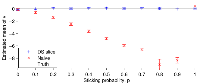
Figure 3: Estimates of the mean of $v$ from the funnel distribution (the true mean is 0) when using slice samplers driven by a dependent, ‘sticky’ stream of random variates. The error bars show $\pm$2 standard errors, using the effective sample size estimated by R-CODA (Plummer et al., 2006). The naive approach uses existing sampling code and treats the stream as if it gave independent uniform outputs, which leads to bias. Our ‘DS slice’ sampler, adapted to dependent streams (Fig. 2), theoretically gives no bias but could mix poorly. In practice, the empirical diagnostics find that our method works equally well (for this task) no matter how sticky the dependent stream is.

Following the setup of Neal (2003), we ran simulations for 240,000 single-variable slice-sampling updates of each variable. Fig. 3 shows the estimated means of the log-variance $v$. When the source stream of random variates never sticks (i.e., when $p\!=\!0$) the estimates of the mean are consistent with the true value of zero. The naive use of the dependent stream in a standard slice sampling code rapidly breaks down, returning confidently wrong answers for $p\!>\!0$.

Our slice sampler, modified for use with the dependent stream by the procedure described in section 5.3, continues to provide good estimates of the mean for the sticky streams. In fact, we obtain good estimates even when the stream always returns a constant and the chain is deterministic (i.e., when $p\!=\!0$). The behavior of trace plots, such as Fig. 4, is indistinguishable from those originally reported in Neal (2003).

This trace plot (Fig. 4) suggests that, for the funnel distribution, the interactions between the updates for each component are complicated enough to explore the distribution without the need for any external randomness. In this deterministic limit, only a countable set of points can be reached by the chain for a given initial condition, and so the chain is not Harris recurrent. Its behavior, however, appears to be indistinguishable from the ergodic chains with $p\!>\!0$.

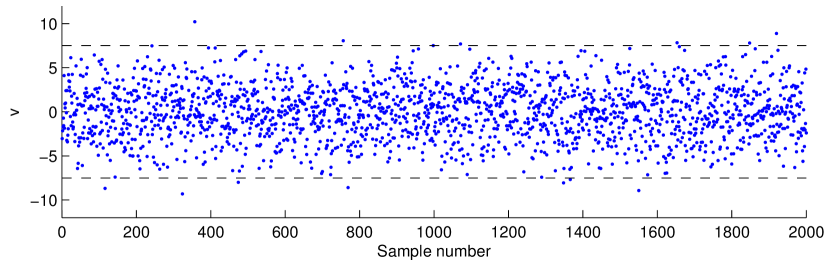
Figure 4: This figure shows samples of $v$ from the funnel distribution, taken after every 120 slice sampling updates of every component of the distribution, to match the bottom pane of Neal’s (2003) Figure 14. We used our dependent stream slice sampler (Fig. 2), using the sticky stream with $p\!=\!1$. That is, after the initialization, no external randomness is added. The pseudo-randomness here is entirely due to the complexity of the slice sampling algorithm itself.

6.2 Dependent streams can improve MCMC algorithms

Dependencies in the noise source used to drive an MCMC algorithm are not necessarily just a problem to be avoided. Introducing dependencies can actually improve MCMC performance. As an example, we consider the artificial problem of sampling uniformly from the integers modulo 100. By symmetry, applying the following update rule to a pair $(x,u)$ will yield a walk that spends equal amounts of time at each integer $x\!\in\!\{0,\dots,99\}$ on average:

1. $d_{1}\sim\mathcal{D},~{}~{}d_{2}\sim\mathcal{D},~{}~{}u\leftarrow\left(u+d_{1}-d_{2}\right)\,\mathrm{mod}~{}1$

2. if $u<0.5$:

3. $x\leftarrow\mathrm{mod}(x+1,100)$

4. else:

5. $x\leftarrow\mathrm{mod}(x-1,100)$

If the random stream $\mathcal{D}$ gives independent uniform variates, then the walk will take around $50^{2}\!=\!2500$ steps to move half way around the ring. However, if adjacent numbers from the stream $\mathcal{D}$ are very similar, then motion of the state will persist in a single direction for a long time. For strong dependencies, the typical time to move half way around the ring is more like $50$ steps, which is 50 times faster.

There is a similarity here with Hamiltonian Monte Carlo methods (e.g., Neal, 2011; Girolami and Calderhead, 2011). In these methods, an auxiliary momentum variable is included in the state space of the chain. A deterministic simulation jointly moves the original and auxiliary variables in a way that reduces random walk behavior of the chain. Hamiltonian dynamics cannot be simulated exactly. Instead, a discrete approximation is performed, which does not itself leave the target distribution invariant and requires correction with a Metropolis step. Standard Hamiltonian dynamics are only defined for differentiable log-densities. It is possible that the methods presented in this paper can use dependencies in random streams to improve mixing in more general problems. Identifying such practical ways to exploit dependencies is an interesting future direction of research.

7 Discussion

We have shown that arbitrary streams of numbers can be used to drive a Markov chain Monte Carlo algorithm that leaves a target distribution invariant. If the stream has sufficient variability, or if a source of ideal random numbers is used occasionally, the algorithm will also be ergodic. This claim may be counter-intuitive: what if an adversary set the numbers in the stream? Given our initial condition, an adversary could make our Markov chain walk to any state of their choosing, including one with incredibly low probability. However, if we replaced the initial condition with another drawn from the target distribution, it is unlikely that the same stream would direct us to an atypical state. The stream of numbers must be picked without looking at the state of our chain, but otherwise it really can be picked arbitrarily.

This work was originally motivated by theoretical neuroscience research into Markov chain Monte Carlo implementations in networks of neurons. The idea that MCMC may be implemented in the brain is present from early neural network models (Alspector et al., 1989), to more recent models of cognition (Ullman et al., 2010) and spiking neurons (Buesing et al., 2011). Our theoretical contribution shows that a source of independent random variates is not required to construct Markov chains for complex target distributions. Indeed a system driven by dependent randomness may even perform better. The particular algorithms suggested here may not be neurally plausible, but it seems unlikely that if MCMC is implemented in the brain, truly independent variates are used.

8 Future work

In certain circumstances, sequences of pseudo-random numbers can be used to obtain consistent estimates from Markov chains (Chentsov, 1967). Recent work has used quasi-random numbers, which are deliberately ‘more uniform’ than pseudo-random numbers, to drive a Metropolis method (Owen and Tribble, 2005), obtaining lower variance estimation in certain circumstances. Our work has a different purpose: we wish to use arbitrary sequences, potentially with any MCMC algorithm, and get an operator that leaves the target distribution invariant. In doing so, we can safely interleave our operators with any other MCMC operators. However, relating our work to that on quasi-Monte Carlo, and trying to exploit dependencies in practice (as suggested in section 6.2) is an interesting future direction.

In this work, we have adopted a model for non-uniform random variate generation that uses continuous random inputs. This model is commonly adopted, although it is also possible to use random bits as input instead (Devroye, 1986). Another interesting future direction might be attempting to sample from a discrete target distribution using a stream of discrete dependent variates.

There are several popular software packages for automatically constructing samplers from user-specified models. Examples include the long-standing BUGS project (Lunn et al., 2009), and more recently, Church (Goodman et al., 2008). Developing our strategy into an automatic code transformation procedure would allow widespread use of Monte Carlo methods that require fewer high-quality random numbers. Such developments may be useful as more large-scale parallel simulations are deployed.

9 Conclusion

For most statistical purposes, current MCMC practice with pseudo-random number generators works well. This situation can change with computational paradigms: for example, care is required when generating many parallel streams of pseudo-random numbers or when pseudo-random numbers are combined with physical sources of entropy. This paper provides a means to make MCMC robust to poor-quality random numbers, and so provides a new standard to check against. Our practical example demonstrated a very long run of a deterministic Markov chain, with no source of randomness at all, that gave useful results. In general it would be wise to randomize at least some of the steps. However, with our modifications, the commonly-perceived need for vast numbers of random variates for MCMC simulations may be illusory.

References

- Alspector et al. (1989) Alspector, J., B. Gupta, and R. B. Allen (1989). Performance of a stochastic learning microchip. In D. S. Touretzky (Ed.), Advances in Neural Information Processing Systems I, pp. 748–760.
- Buesing et al. (2011) Buesing, L., J. Bill, B. Nessler, and W. Maass (2011). Neural dynamics as sampling: A model for stochastic computation in recurrent networks of spiking neurons. PLoS Computational Biology 7(11), e1002211.
- Chentsov (1967) Chentsov, N. N. (1967). Pseudorandom numbers for modelling Markov chains. USSR Computational Mathematics and Mathematical Physics 7(3), 218–233.
- Devroye (1986) Devroye, L. (1986). Non-uniform random variate generation. Springer–Verlag.
- Entacher (1998) Entacher, K. (1998). Bad subsequences of well-known linear congruential pseudorandom number generators. ACM Transactions on Modeling and Computer Simulation 8(1), 61–70.
- Gärtner (2000) Gärtner, B. (2000). Pitfalls in computing with pseudorandom determinants. In Proceedings of the sixteenth annual symposium on Computational geometry, pp. 148–155.
- Gilks (1992) Gilks, W. R. (1992). Derivative-free adaptive rejection sampling for Gibbs sampling. In J. Bernardo, J. Berger, A. P. Dawid, and A. F. M. Smith (Eds.), Bayesian Statistics 4, pp. 337–348.
- Gilks and Wild (1992) Gilks, W. R. and P. Wild (1992). Adaptive rejection sampling for Gibbs sampling. Applied Statistics 41(2), 337–348.
- Girolami and Calderhead (2011) Girolami, M. and B. Calderhead (2011). Riemann manifold Langevin and Hamiltonian Monte Carlo methods. Journal of the Royal Statistical Society, Series B 73(2), 123–214.
- Goodman et al. (2008) Goodman, N. D., V. K. Mansinghka, D. M. Roy, K. Bonawitz, and J. B. Tenenbaum (2008). Church: a language for generative models. In Proceedings of the Twenty-Fourth Conference Annual Conference on Uncertainty in Artificial Intelligence, pp. 220–229.
- Green (1995) Green, P. J. (1995). Reversible jump Markov chain Monte Carlo computation and Bayesian model determination. Biometrika 82(4), 711–732.
- Gutterman et al. (2006) Gutterman, Z., B. Pinkas, and T. Reinman (2006). Analysis of the Linux random number generator. In IEEE Symposium on Security and Privacy, pp. 371–385.
- Hastings (1970) Hastings, W. K. (1970). Monte Carlo sampling methods using Markov chains and their applications. Biometrika 57(1), 97–109.
- Jun and Kocher (1999) Jun, B. and P. Kocher (1999). The Intel random number generator. Cryptography Research Inc., White Paper.
- Lunn et al. (2009) Lunn, D., D. Spiegelhalter, A. Thomas, and N. Best (2009). The BUGS project: evolution, critique and future directions. Statistics in Medicine 4(30), 3049–3067.
- Neal (2000) Neal, R. (2000). Markov chain sampling methods for Dirichlet process mixture models. Journal of computational and graphical statistics 9(2), 249–265.
- Neal (1993) Neal, R. M. (1993). Probabilistic inference using Markov chain Monte Carlo methods. Technical Report CRG-TR-93-1, Department of Computer Science, University of Toronto.
- Neal (2004) Neal, R. M. (1995–2004). Software for flexible Bayesian modeling and Markov chain sampling (FBM). Available from: http://www.cs.toronto.edu/~radford/fbm.software.html.
- Neal (2003) Neal, R. M. (2003). Slice sampling. Annals of Statistics 31(3), 705–767.
- Neal (2011) Neal, R. M. (2011). MCMC using Hamiltonian dynamics. In Handbook of Markov Chain Monte Carlo, pp. 113–143. Chapman & Hall / CRC Press.
- Owen and Tribble (2005) Owen, A. and S. Tribble (2005). A quasi-Monte Carlo Metropolis algorithm. Proceedings of the National Academy of Sciences of the United States of America 102(25), 8844–8849.
- Plummer et al. (2006) Plummer, M., N. Best, K. Cowles, and K. Vines (2006). CODA: Convergence diagnosis and output analysis for MCMC. R News 6(1), 7–11.
- Press et al. (2002) Press, W. H., S. A. Teukolsky, W. T. Vetterlin, and B. P. Flannery (2002). Numerical recipes in C. Cambridge University Press.
- Savicky (2006) Savicky, P. (2006). A strong nonrandom pattern in Matlab default random number generator. Manuscript available from http://www2.cs.cas.cz/~savicky/papers/.
- Shaltiel (2002) Shaltiel, R. (2002). Recent developments in explicit constructions of extractors. Bulletin of the European Association For Theoretical Computer Science 77, 67–95.
- Skilling (2004) Skilling, J. (2004). BayeSys and MassInf. Maximum Entropy Data Consultants Ltd.
- Tierney (1994) Tierney, L. (1994). Markov chains for exploring posterior distributions. The Annals of Statistics 22(4), 1701–1728.
- Ullman et al. (2010) Ullman, T. D., N. D. Goodman, and J. B. Tenenbaum (2010). Theory acquisition as stochastic search. In Proceedings of the 32nd Annual Conference of the Cognitive Science Society, pp. 2840–2845.