Asymptotic expansions for high-contrast elliptic equations

1 Abstract

In this paper, we present a high-order expansion for elliptic equations in high-contrast media. The background conductivity is taken to be one and we assume the medium contains high (or low) conductivity inclusions. We derive an asymptotic expansion with respect to the contrast and provide a procedure to compute the terms in the expansion. The computation of the expansion does not depend on the contrast which is important for simulations. The latter allows avoiding increased mesh resolution around high conductivity features. This work is partly motivated by our earlier work in [22] where we design efficient numerical procedures for solving high-contrast problems. These multiscale approaches require local solutions and our proposed high-order expansion can be used to approximate these local solutions inexpensively. In the case of a large-number of inclusions, the proposed analysis can help to design localization techniques for computing the terms in the expansion. In the paper, we present a rigorous analysis of the proposed high-order expansion and estimate the remainder of it. We consider both high and low conductivity inclusions.

2 Introduction

The mathematical analysis and numerical analysis of partial differential equations in high-contrast and multiscale media are important for many practical applications. For instance, in porous media applications, the permeability of subsurface regions is described as a quantity with high-contrast and multiscale features. A main goal is to understand the effects and complexity related to this multiscale variation and high-contrast in the coefficients. This is specially important for the computation of numerical solutions and quantities of interest. Many tools and methods have been developed and used to study high contrast problems. We mention few recent works where numerical methods are designed that target problems with difficult variation in the coefficients. The numerical analysis of these methods require accurate descriptions of the variation of the coefficients. In [19, 10, 12, 13, 31, 2, 8, 7, 36, 37] multiscale methods for problems with high-contrast coefficients are described. For domain decomposition methods with discontinuous coefficients we mention [34, 15, 30, 35, 28] and references therein. Some domain decomposition techniques for multiscale partial differential equations with complicated variations in the coefficients are developed in [29, 18, 24, 33, 22, 16, 23]. Additionally, we mention [11, 17, 38] among others, which focus on multilevel methods targeting problems with high-contrast and discontinuous coefficients. Numerical methods based on different asymptotic analysis are detailed in [4, 21, 27, 14, 9].

In the case of elliptic problems with oscillating coefficients and bounded contrast, multiscale methods and homogenizations techniques have been successfully applied to study solutions of elliptic differential equations (c.f., [20, 3, 32] and references therein). Many homogenization and multiscale methods start with the derivation of an asymptotic expansion for the solution of the partial differential equation. The expansion is written in terms of the problem parameter(s): e.g., the period in the case of oscillating periodic coefficients. The asymptotic expansion is then used to study the problem at hand.

In this paper and in the same spirit, we derive asymptotic expansions for the solutions of elliptic problems with high-contrast. In this case the parameter to be consider is the contrast in the coefficient. In particular, we consider the problem

$$-\mbox{div}(\kappa(x)\nabla u)=f,\mbox{ in }D$$ (1)

with Dirichlet data given by $u=g$ on $\partial D$. We assume that $\kappa(x)>0$. The contrast in the coefficient, $\|\kappa\|_{L^{\infty}(D)}\|\kappa^{-1}\|_{L^{\infty}(D)}$, is the important parameter considered here. For the analysis, we consider a binary media $\kappa(x)$ with background one and with multiple (connected) inclusions. We consider high-conductivity inclusions (with conductivity $\eta$) and low-conductivity inclusions (with conductivity $1/\eta$). We derive expansions of the form

$$u_{\eta}=\eta u_{-1}+u_{0}+\frac{1}{\eta}u_{1}+\frac{1}{\eta^{2}}u_{2}+\dots.$$ (2)

In the case with only high-conductivity inclusions we have $u_{-1}=0$ and (2) reduces to

$$u_{\eta}=u_{0}+\frac{1}{\eta}u_{1}+\frac{1}{\eta^{2}}u_{2}+\dots.$$ (3)

In the presence of low-conductivity inclusions we may have $u_{-1}\not=0$ depending on the support of the forcing term. We mention here that, in order to derive the expansions, we use the weak formulation associated to (1). In this case, using the integral formulation has the advantage that the boundary, interface and transmission conditions are self-revealing.

The asymptotic problems for the case of only high-conductivity or only low-conductivity are studied in detail. For the study of the high-conductivity inclusions asymptotic problem we use harmonic characteristic functions. These functions are defined as being constant inside the inclusions and harmonic in the background domain. The asymptotic solution can be obtained by solving a Dirichlet problem in the background domain and a finite dimensional problem in the space spanned by the harmonic characteristic functions. The solution of the finite dimensional problem gives a closed formula for the constant values of the limit solution inside the high-conductivity inclusions. The resulting system can be large, in general, and one can consider some localization techniques (c.f., [4, 5]).

The asymptotic problem and approximations of the asymptotic problem, in the case of high-conductivity inclusions, have been studied in the literature. We mention [4, 6, 9] where a discrete network approximation is considered for the problem of computing the effective conductivity of high-contrast, randomly, and densely packed composites with high-conductivity inclusions. The network approximation depends on the geometry of the inclusions and the behavior of the solution between nearby inclusions. The authors can localize the interaction of high-conductivity inclusions using graph-theoretical concepts. Furthermore, they propose a finite element approach for solving the resulting system and identifying the first order approximation of the solution. In [5] the authors study the homogenization of the asymptotic problem in terms of geometric parameters such as the shapes of inclusions and the distance between the inclusions. They develop an asymptotic analysis for periodic structures with absolutely conductive square inclusions. The small scales considered here are the period of the structure and the distance between inclusions. We refer to the works [4, 5, 6] and references therein.

We also write a low-conductivity asymptotic problem valid only in the case where the forcing term vanishes inside the low-conductivity inclusions. This problem is important in flow applications where low conductivity regions represent shale regions and can substantially alter the overall flow behavior. To our best knowledge, this problem is not extensively studied in the literature. The asymptotic solution can be obtained by solving: 1) a mixed boundary condition problem in the background domain, and then, 2) a Dirichlet problem inside the inclusion with zero forcing term and the Dirichlet data from 1).

We show how to obtain all the coefficients in the expansions. The procedure to compute the coefficients, coincide with a Dirichlet-to-Neumann procedure as in Domain Decompositions Methods; see [28, 35]. For the case of high-conductivity inclusions, the Neumann problems are solved in the interior inclusions and therefore, a compatibility condition needs to be verified. Obtaining the right balance of fluxes for the compatibility condition involves the solution of a finite dimensional problem in the space spanned by the harmonic characteristic functions mentioned above. For the case of low-conductivity inclusions the Neumann problems are solved in the background domain and no compatibility condition in required. The expansions derived in this paper are proven to converge in $H^{1}(D)$ for high-contrast bigger that a certain constant. This constant depends on the domains representing the inclusions and the background domain. Asymptotic expansions in the presence of boundary intersecting inclusions can be derived and analyzed using similar arguments. The presence of low- and high-conductivity inclusions can be also analyzed. More general geometrical configurations and partial differential equations can be studied as well.

Having a practical procedure to compute the next leading order terms in (2) is useful for applications. For instance, the quantity $u_{1}$ in (3) may have considerable contribution to some quantity of interest in some regions, e.g., in the velocity $\kappa|\nabla u_{\eta}|$ expansion, the solution is multiplied by $\eta$. A high-order expansion is also useful when constructing multiscale and multilevel methods. The expansion (2) can be used to construct multiscale finite element basis functions; see [20, 12]. Such an expansion will allow the construction of basis functions independent of the contrast and depending only on the limiting problem. In the case of expansion (2), the asymptotic problem depends only on the geometry configuration describing the inclusions (see Section 4.3.1). These basis functions will capture the effect on the solution of the geometric arrangement describing the conductivity. The next order terms in (2) can be used to construct correction terms to account for the effect of the contrast in the coefficient. Expansion (2) can be used to improve existing advanced multiscale finite element techniques for a better sub-grid capturing; see [10, 20]. Fast numerical upscaling techniques can also be constructed with the first order terms of (2) or (3). See [21] where the authors develop fast numerical upscaling methods based on some asymptotic analysis. We also mention [27, 14] where numerical approximations are designed using asymptotic analysis.

The rest of the paper is organized as follows. In Section 3 we recall the weak formulation of (1). In Section 4 we derive the expansion for the case of high-conductivity inclusions. We study the asymptotic problem and the convergence of the expansions. Section 5 is dedicated to the case of low-conductivity inclusions. In Section 6 we consider the case with low- and high-conductivity inclusions and in Section 7 we make some conclusion and final comments.

3 Problem Setting

Let $D\subset\mathbb{R}^{d}$ polygonal domain or a domain with smooth boundary. We consider the following weak formulation of (1). Find $u\in H^{1}(D)$ such that

$$\left\{\begin{array}[]{ll}a(u,v)=f(v)&\forall v\in H_{0}^{1}(D),\\ \hskip 21.68121ptu=g&\mbox{ on }\partial D.\end{array}\right.$$ (4)

Here the bilinear form $a$ and the linear functional $f$ are defined by

$$a(u,v) =\int_{D}\kappa(x)\nabla u(x)\cdot\nabla v(x) \forall u,v\in H_{0}^{1}(D)$$ (5)

$$f(v) =\int_{D}f(x)v(x) \forall v\in H_{0}^{1}(D).$$ (6)

We assume that $D$ is the disjoint union of a background domain and inclusions, $D=D_{0}\cup(\cup_{m=1}^{M}D_{m}).$ We assume that $D_{0},D_{1},\dots,D_{M},$ are polygonal domains (or domains with smooth boundaries). We also assume that each $D_{m}$ is a connected domain, $m=0,1,\dots,M$. Let $D_{0}$ represent the background domain and the subdomains $\{D_{m}\}_{m=1}^{M}$ represent the inclusions. For simplicity of the presentation we consider only interior inclusions. See Figure 1 for two dimensional illustrations.

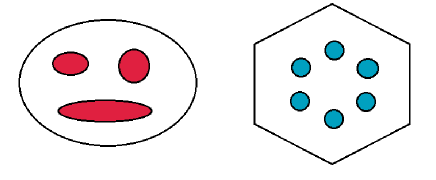
Figure 1: Examples of geometry configurations with interior inclusions.

Given $w\in H^{1}(D)$ we will use the notation $w^{(m)}$, for the restriction of $w$ to the domain $D_{m}$, that is,

$$w^{(m)}=w|_{D_{m}},\quad m=0,1,\dots,M.$$

4 Expansions for high-conductivity inclusions

In this section we derive and analyze expansions for the case of high conductivity inclusions. For the sake of readability and presentation, we consider first the case of only one high-conductivity inclusion in Section 4.1 and study the convergence of this expansion in Section 4.2. We present the multiple high-conductivity inclusions case in Section 4.3, where we describe the expansion and analyze its convergence, following the structure presented in Sections 4.1 and 4.2.

4.1 Derivation for one high-conductivity inclusion

Let $\kappa$ be defined by

$$\kappa(x)=\left\{\begin{array}[]{cc}\eta,&x\in D_{1},\\ 1,&x\in D_{0}=D\setminus\overline{D}_{1},\end{array}\right.$$ (7)

and denote by $u_{\eta}$ the solution of the weak formulation  (4). We assume that $D_{1}$ is compactly included in $D$ ($\overline{D}_{1}\subset D$). Since $u_{\eta}$ is solution of (4) with the coefficient (7), we have

$$\int_{D_{0}}\nabla u_{\eta}\cdot\nabla v+\eta\int_{D_{1}}\nabla u_{\eta}\cdot\nabla v=\int_{D}fv\quad\forall v\in H_{0}^{1}(D).$$ (8)

We seek to determine $\{u_{i}\}_{i=0}^{\infty}\subset H^{1}(D)$ such that,

$$u_{\eta}=u_{0}+\frac{1}{\eta}u_{1}+\frac{1}{\eta^{2}}u_{2}+\dots=\sum_{i=0}^{\infty}\eta^{-i}u_{i},$$ (9)

and such that they satisfy the following Dirichlet boundary conditions,

$$u_{0}=g\mbox{ on }\partial D\quad\mbox{ and }\quad u_{i}=0\mbox{ on }\partial D\mbox{ for }i\geq 1.$$ (10)

We substitute (9) into (8) to obtain that for all $v\in H^{1}_{0}(D)$ we have,

$$\sum_{i=0}^{\infty}\eta^{-i}\int_{D_{0}}\nabla u_{i}\cdot\nabla v+\sum_{i=0}^{\infty}\eta^{-i+1}\int_{D_{1}}\nabla u_{i}\cdot\nabla v=\int_{D}fv$$

or

$$\eta\int_{D_{1}}\nabla u_{0}\cdot\nabla v+\sum_{i=0}^{\infty}\eta^{-i}\left(\int_{D_{0}}\nabla u_{i}\cdot\nabla v+\int_{D_{1}}\nabla u_{i+1}\cdot\nabla v\right)=\int_{D}fv.$$ (11)

Now we collect terms with equal powers of $\eta$ and analyze the resulting subdommain equations.

4.1.1 Term corresponding to $\eta=\eta^{1}$

In (11) there is one term corresponding to $\eta$ to the power 1, thus we obtain the following equation

$$\int_{D_{1}}\nabla u_{0}\cdot\nabla v=0\mbox{ for all }v\in H^{1}_{0}(D).$$ (12)

In the general case, the meaning of this equation depends on the relative position of the inclusion $D_{1}$ with respect to the boundary. It may need to take the boundary data into account. Since we are assuming that $\overline{D}_{1}\subset D$, we conclude that $\nabla u_{0}^{(1)}=0$ in $D_{1}$ and then $u_{0}^{(1)}$ (the restriction of $u_{0}$ on $D_{1}$) is a constant.

4.1.2 Terms corresponding to $\eta^{0}=1$

Equation (11) contains three terms corresponding to $\eta$ to the power 0, which are:

$$\int_{D_{0}}\nabla u_{0}\cdot\nabla v+\int_{D_{1}}\nabla u_{1}\cdot\nabla v=\int_{D}fv\mbox{ for all }v\in H^{1}_{0}(D).$$ (13)

Let

$$V_{const}=\{v\in H^{1}_{0}(D),\mbox{ such that }v^{(1)}=v|_{D_{1}}\mbox{ is constant}\}.$$

If we consider $z\in V_{const}$ in equation (13) we conclude that $u_{0}$ satisfies the following problem,

$$\displaystyle\left(\int_{D}\nabla u_{0}\cdot\nabla z=\right)\quad\int_{D_{0}}\nabla u_{0}\cdot\nabla z =\int_{D}fz \forall z\in V_{const}$$ (14)

$$u_{0} =g \mbox{ on }\partial D$$ (15)

The problem (14) is elliptic and it has a unique solution. To analyze this problem further, it is natural to define a harmonic characteristic function $\chi_{D_{1}}\in H^{1}_{0}(D)$ such that

$$\chi_{D_{1}}^{(1)}=1\quad\mbox{ in }D_{1},$$

and the harmonic extension of its boundary data in $D_{0}$ is given by

$$\displaystyle\int_{D_{0}}\nabla\chi_{D_{1}}^{(0)}\cdot\nabla z =0 \forall z\in H^{1}_{0}(D_{0})$$

$$\chi_{D_{1}}^{(0)} =1 \mbox{ on }\partial D_{1},$$ (16)

$$\chi_{D_{1}}^{(0)} =0 \mbox{ on }\partial D.$$

To obtain an explicit formula for $u_{0}$ we will use the following facts: $(i)$ problem (14) is elliptic and has a unique solution, and $(ii)$ a property of the harmonic characteristic functions described in the Remark below.

Remark 1

Let $w$ be a harmonic extension to $D_{0}$ of its Neumann data on $\partial D_{0}$. That is, $w$ satisfy the following problem,

$$\int_{D_{0}}\nabla w\cdot\nabla z=\int_{\partial D_{0}}\nabla w\cdot n_{0}\,z\quad\mbox{ for all }z\in H^{1}(D_{0}).$$

Since $\chi_{D_{1}}=0$ on $\partial D$ and $\chi_{D_{1}}=1$ on $\partial D_{1}$, we readily have that

$$\int_{D_{0}}\nabla\chi_{D_{1}}\cdot\nabla w=\int_{\partial D_{0}}\nabla w\cdot n\chi_{D_{1}}=0\left(\int_{\partial D}\nabla w\cdot n\right)+1\left(\int_{\partial D_{1}}\nabla w\cdot n_{0}\right)$$

and we conclude that for every harmonic function on $D_{0}$,

$$\int_{D_{0}}\nabla\chi_{D_{1}}\cdot\nabla w=\int_{\partial D_{1}}\nabla w\cdot n_{0}.$$ (17)

In particular, taking $w=\chi_{D_{1}}$ we have:

$$\int_{D}|\nabla\chi_{D_{1}}|^{2}=\int_{D_{0}}|\nabla\chi_{D_{1}}|^{2}=\int_{\partial D_{1}}\nabla\chi_{D_{1}}\cdot n_{0}.$$ (18)

Note also that if $\xi\in H^{1}(D)$ is such that $\xi^{(1)}=\xi|_{D_{1}}=c$ is constant in $D_{1}$ and $\xi^{(0)}=\xi|_{D_{0}}$ is harmonic in $D_{0}$, then, $\xi=c\chi_{D_{1}}$.

We can decompose $u_{0}$ into the harmonic extension of its constant value in $D_{1}$, $c(u_{0})$, plus the remainder $u_{0,0}\in H^{1}(D_{0})$. Thus, we write,

$$u_{0}=u_{0,0}+c(u_{0})\chi_{D_{1}}$$

where $u_{0,0}\in H^{1}(D)$ is defined by $u_{0,0}^{(1)}=0$ in $D^{(1)}$ and $u_{0,0}^{(0)}$ solves the following Dirichlet problem,

$$\displaystyle\int_{D_{0}}\nabla u_{0,0}^{(0)}\cdot\nabla z =\int_{D_{0}}fz \forall z\in H^{1}_{0}(D_{0}).$$ (19)

$$u_{0,0}^{(0)} =0 \mbox{ on }\partial D_{1},$$

$$u_{0,0}^{(0)} =g \mbox{ on }\partial D.$$

From equation (14) and the observations in Remark 1 we get that

$$\int_{D_{0}}\nabla(u_{0,0}+c(u_{0})\chi_{D_{1}})\cdot\nabla\chi_{D_{1}}=\int_{D}f\chi_{D_{1}}$$

from which we can obtain

$$c(u_{0})=\frac{\int_{D}f\chi_{D_{1}}-\int_{D_{0}}\nabla u_{0,0}\cdot\nabla\chi_{D_{1}}}{\int_{D_{0}}|\nabla\chi_{D_{1}}|^{2}}.$$ (20)

There is a useful alternative expression for $c(u_{0})$ in (20) that we also use. By using the Neumann problem related to $u_{0,0}$ we have that,

$$\int_{D_{0}}\nabla u_{0,0}\cdot\nabla\chi_{D_{1}} = \int_{D_{0}}f\chi_{D_{1}}+\int_{\partial D_{0}}\nabla u_{0,0}\cdot n_{0}\chi_{D_{1}}$$

$$= \int_{D_{0}}f\chi_{D_{1}}+\int_{\partial D_{1}}\nabla u_{0,0}\cdot n_{0}1$$

and then noting that $\int_{D}f\chi_{D_{1}}=\int_{D_{0}}f\chi_{D_{1}}+\int_{D_{1}}f$ we get,

$$c(u_{0})=\dfrac{\int_{D_{1}}f-\int_{\partial D_{1}}\nabla u_{0,0}\cdot n_{0}}{\int_{\partial D_{1}}\nabla\chi_{D_{1}}\cdot n_{0}},$$ (21)

which reveals that $c(u_{0})$ balances the fluxes across $\partial D_{1}$. To summarize the results obtained to this point, we can express $u_{0}$ as follows:

$$u_{0} =u_{0,0}+\dfrac{\int_{D}f\chi_{D_{1}}-\int_{D_{0}}\nabla u_{0,0}\cdot\nabla\chi_{D_{1}}}{\int_{D_{0}}|\nabla\chi_{D_{1}}|^{2}}\chi_{D_{1}}$$ (22)

$$=u_{0,0}+{\dfrac{\int_{D_{1}}f-\int_{\partial D_{1}}\nabla u_{0,0}\cdot n_{0}}{\int_{\partial D_{1}}\nabla\chi_{D_{1}}\cdot n_{0}}}\chi_{D_{1}}$$ (23)

Given the explicit form of $u_{0}$, we use it in (13) to find $u_{1}^{(1)}=u_{1}|_{D_{1}}$, from if we conclude that $u_{0}^{(0)}$ and $u_{1}^{(1)}$ satisfy the local Dirichlet problems

$$\int_{D_{0}}\nabla u_{0}\cdot\nabla z =\int_{D_{0}}fz \forall z\in H^{1}_{0}(D_{0}),$$

$$\int_{D_{1}}\nabla u_{1}\cdot\nabla z =\int_{D_{1}}fz \forall z\in H^{1}_{0}(D_{1}),$$

with given boundary data on $\partial D_{0}$ and $\partial D_{1}$. Equation (13) also represents the transmission conditions across $\partial D_{1}$ for the functions $u_{0}^{(0)}$ and $u_{1}^{(1)}$. This is easier to see when the forcing $f$ is square integrable. From now on, in order to simplify the presentation, we assume that $f\in L^{2}(D)$. If $f\in L^{2}(D)$, we have that $u_{0}^{(0)}$ and $u_{1}^{(1)}$ are the only solutions of the problems:

$$\int_{D_{0}}\nabla u_{0}^{(0)}\cdot\nabla z=\int_{D_{0}}fz+\int_{\partial{D_{0}}\setminus\partial D}\nabla u_{0}^{(0)}\cdot n_{0}z\quad\forall z\in H^{1}({D_{0}})\mbox{ with }z=0\mbox{ on }\partial D$$

with $u_{0}^{(0)}={g}$ on $\partial D$, and

$$\int_{D_{1}}\nabla u_{1}^{(1)}\cdot\nabla z=\int_{D_{1}}fz+\int_{\partial D_{1}}\nabla u_{1}^{(1)}\cdot n_{1}z\quad\mbox{ for all }z\in H^{1}(D_{1}).$$

Replacing these last two equations back into (13) we conclude that

$$\int_{\partial D_{1}}(\nabla u_{0}^{(0)}\cdot n_{0}+\nabla u_{1}^{(1)}\cdot n_{1})z=0\quad\mbox{ for all }z\in H^{1}(D),$$

which implies

$$\nabla u_{1}^{(1)}\cdot n_{1}=-\nabla u_{0}^{(0)}\cdot n_{0}\quad\mbox{ on }\partial D_{1}.$$

Using this interface condition we can obtain $u_{1}^{(1)}$ in $D_{1}$ by writing

$$u_{1}^{(1)}=\widetilde{u}_{1}^{(1)}+c_{1}\quad\mbox{ where }\int_{D_{1}}\widetilde{u}_{1}^{(1)}=0$$

and $\widetilde{u}_{1}^{(1)}$ solves the Neumann problem

$$\int_{D_{1}}\nabla\widetilde{u}_{1}^{(1)}\cdot\nabla z=\int_{D_{1}}fz-\int_{\partial D_{1}}\nabla u_{0}^{(0)}\cdot n_{1}z\quad\mbox{ for all }z\in H^{1}(D_{1}).$$ (24)

The constant $c_{1}$ will be chosen later. Problem (24) satisfies the compatibility condition,

$$\int_{\partial D_{1}}\nabla\widetilde{u}_{1}^{(1)}\cdot n_{1} = -\int_{\partial D_{1}}\nabla u_{0}^{(0)}\cdot n_{0}$$

$$= -\int_{\partial D_{1}}\nabla u_{0}^{(0)}\cdot n_{0}-c(u_{0})\int_{\partial D}\nabla\chi_{D_{1}}\cdot n_{0}=\int_{D_{1}}f.$$

Here we use the value of $c(u_{0})$ is given in (21).

Next, we discuss how to compute $u_{1}^{(0)}$ and $\widetilde{u}_{1}^{(0)}$ to completely define the functions $u_{1}\in H^{1}(D)$ and $\widetilde{u}_{1}\in H^{1}(D)$. These are presented for general $i\geq 1$ since the construction is independent of $i$ in this range.

4.1.3 Term corresponding to $\eta^{-i}$ with $i\geq 1$:

For powers of ${1}/{\eta}$ larger or equal to one there are only two terms in the summation that lead to the following system:

$$\int_{D_{0}}\nabla u_{i}\cdot\nabla v+\int_{D_{1}}\nabla u_{i+1}\cdot\nabla v=0\quad\mbox{ for all }v\in H^{1}_{0}(D).$$ (25)

This equation represents both the subdomain problems and the transmission conditions across $\partial D_{1}$ for $u_{i}^{(0)}$ and $u_{i+1}^{(1)}$. Following a similar argument to the one given above, we conclude that $u_{i}^{(0)}$ is harmonic in $D_{0}$ for all $i\geq 1$ and that $u_{i}^{(1)}$ is harmonic in $D_{1}$ for $i\geq 2$. As before, we have

$$\nabla u_{i+1}^{(1)}\cdot n_{1}=-\nabla u_{i}^{(0)}\cdot n_{0}.$$ (26)

We note that $u_{i}^{(1)}$ in $D_{1}$, (e.g., $u_{1}^{(1)}$ above) is given by the solution of a Neumann problem in $D_{1}$. To uniquely determine $u_{i}^{(1)}$, we impose the condition $\int_{D_{1}}u_{i}^{(1)}=c_{i}$ and write

$$u_{i}^{(1)}=\widetilde{u}_{i}^{(1)}+c_{i}\quad\mbox{ where }\int_{D_{1}}\widetilde{u}_{i}=0.$$ (27)

where the appropriate $c_{i}$ will be determined later.

Given $u_{i}^{(1)}$ in $D_{1}$ we find $u_{i}^{(0)}$ in $D_{0}$ by solving a Dirichlet problem with known Dirichlet data, that is,

$$\begin{array}[]{l}\displaystyle\int_{D_{0}}\nabla u_{i}^{(0)}\cdot\nabla z=0\mbox{ for all }z\in H^{1}_{0}(D_{0})\\ \\ u_{i}^{(0)}=u_{i}^{(1)}~{}~{}(=\widetilde{u}_{i}^{(1)}+c_{i})\mbox{ on }\partial D_{1}\quad\mbox{ and }\quad u_{i}=0\mbox{ on }\partial D.\end{array}$$ (28)

Since $c_{i}$, $i=1,\dots,$ are constants, their harmonic extensions are given by $c_{i}\chi_{D_{1}}$, $i=1,\dots$; see Remark 1. Then, we conclude that

$$u_{i}=\widetilde{u}_{i}+c_{i}\chi_{D_{1}}$$ (29)

where $\widetilde{u}_{i}^{(0)}$ is defined by (28) replacing $c_{i}$ by $0$. This completes the construction of $u_{i}$.

Now we proceed to show how to to find $u_{i+1}^{(1)}$ in $D_{1}$. For this, we use (25) and (26) which lead to the following Neumann problem

$$\int_{D_{1}}\nabla\widetilde{u}_{i+1}^{(1)}\cdot\nabla z=-\int_{\partial D_{1}}\nabla u_{i}^{(0)}\cdot n_{0}z\quad\mbox{ for all }z\in H^{1}(D_{1}).$$ (30)

The compatibility condition for this Neumann problem is satisfied if we choose

$$c_{i}=-\frac{\int_{\partial D_{1}}\nabla\widetilde{u}_{i}^{(0)}\cdot n_{0}}{\int_{\partial D_{1}}\nabla\chi_{D_{1}}^{(0)}\cdot n_{0}}=-\frac{\int_{D_{0}}\nabla\widetilde{u}_{i}\cdot\nabla\chi_{D_{1}}}{\int_{D_{0}}|\nabla\chi_{D_{1}}|^{2}}.$$ (31)

For the second equality see Remark 1 below and Equations (20) and (21). The compatibility conditions trivially satisfy

$$\int_{\partial D_{1}}\nabla\widetilde{u}_{i+1}^{(1)}\cdot n_{1} =-\int_{\partial D_{1}}\nabla u_{i}^{(0)}\cdot n_{0}$$

$$=-\int_{\partial D_{1}}\nabla(\widetilde{u}_{i}^{(0)}+c_{i}\chi_{D_{1}}^{(0)})\cdot n_{0}$$

$$=-\int_{\partial D_{1}}\nabla\widetilde{u}_{i}^{(0)}\cdot n_{0}-c_{i}\int_{\partial D_{1}}\nabla\chi_{D_{1}}^{(0)}\cdot n_{0}$$

$$=0.$$

where we have used the definitions of $c_{i}$ given in (31).

We can choose $u_{i+1}^{(1)}$ in $D_{1}$ such that

$$u_{i}^{(1)}=\widetilde{u}_{i+1}^{(1)}+c_{i+1}\quad\mbox{ where }\int_{D_{1}}\widetilde{u}_{i+1}=0,$$

and, as before,

$$c_{i+1}=-\frac{\int_{\partial D_{1}}\nabla\widetilde{u}_{i+1}^{(0)}\cdot n_{0}}{\int_{\partial D_{1}}\nabla\chi_{D_{1}}^{(0)}\cdot n_{0}}=-\frac{\int_{D_{0}}\nabla\widetilde{u}_{i+1}\cdot\nabla\chi_{D_{1}}}{\int_{D_{0}}|\nabla\chi_{D_{1}}|^{2}},$$

so we have the compatibility condition of the Neumann problem to compute $u_{i+2}^{(1)}$. See the Equation (30).

4.1.4 Summary

We summarize the Dirichlet-to-Neumann procedure to compute the terms of the asymptotic expansion for $u_{\eta}$ in (9)-(10).

1. Compute $u_{0}$ using formulae (22) or (23).

2. Compute $u_{1}^{(1)}$ in $D_{1}$ by solving the Neumann problem (24). Compute $u_{1}^{(0)}$ in $D_{0}$ solving the Dirichlet problem (28) with $i=1$.

3. For $i=2,3,\dots$ compute $u_{i}^{(1)}$ in $D_{1}$ by solving the Neumann problem (30). Then, compute $u_{i}^{(0)}$ in $D_{0}$ solving the Dirichlet problem (28).

Other cases can be considered. For instance, an expansion for the case where we interchange $D_{0}$ and $D_{1}$ can also be analyzed. In this case the asymptotic solution is not constant in the high-conducting part. Multiple inclusions will be consider in Section 4.3.

4.2 Convergence in $H^{1}(D)$

In this section we study the convergence of the expansion (9)-(10). For simplicity of the presentation we consider the case of one high-conductivity inclusion. The converge results will be extended to the multiple high-conductivity inclusions in Section 4.3. We assume that $\partial D$ and $\partial D_{1}$ are sufficiently smooth, see [25].

Lemma 2

Let $u_{0}$ in (22), with $u_{0,0}$ defined in (19), and $u_{1}$ be defined by (24) and (28) with $i=1$. We have that,

$$|u_{0}|_{H^{1}(D)}\preceq\|f\|_{H^{-1}(D)}+\|g\|_{H^{1/2}(\partial D)},$$ (32)

$$\|\widetilde{u}_{1}\|_{H^{1}(D_{1})} \preceq \|f\|_{H^{-1}(D_{1})}+\|g\|_{H^{1/2}(D)}$$ (33)

and

$$\|\widetilde{u}_{1}\|_{H^{1}(D_{0})}\preceq\|\widetilde{u}_{1}\|_{H^{1/2}(\partial D_{1})}\preceq\|\widetilde{u}_{1}\|_{H^{1}(D_{1})}.$$ (34)

Proof. From the definition of $u_{0,0}$ in (19) we have that

$$\|u_{0,0}\|_{H^{1}(D_{0})}\preceq\|f\|_{H^{-1}(D_{0})}+\|g\|_{H^{1/2}(\partial D)}.$$

Using (22) we have that

$$|u_{0}|_{H^{1}(D)} = |u_{0}|_{H^{1}(D_{0})}\leq|u_{0,0}|_{H^{1}(D_{0})}+|c(u_{0})||\chi_{D_{1}}|_{H^{1}(D_{0})}$$ (35)

and we observe that

$$|c(u_{0})||\chi_{D_{1}}|_{H^{1}(D_{0})} \preceq |\frac{\int_{D}f\chi_{D_{1}}-\int_{D_{0}}\nabla u_{0,0}\cdot\nabla\chi_{D_{1}}}{|\chi_{D_{1}}|_{H^{1}(D_{0})}}|$$

$$\preceq \|f\|_{H^{-1}(D)}+\|g\|_{H^{1/2}(\partial D)}.$$

This proves (32). Equation (33) follows from the classical estimate for problem (24). Equation (34) follows from problem (28) with $i=1$ and a trace theorem; see [25].  

The following lemma can be obtained using orthogonality relations of Galerkin projections.

Lemma 3

If $\widetilde{w}\in H^{1}(D)$, $\widetilde{w}$ is harmonic in $D_{0}$ and we define

$$w=\widetilde{w}+c(w)\chi_{D_{1}}$$

where

$$c(w)=-\frac{\int_{\partial D_{1}}\nabla\widetilde{w}\cdot n_{0}}{\int_{\partial D_{1}}\nabla\chi_{D_{1}}\cdot n_{0}}=-\frac{\int_{D_{0}}\nabla\widetilde{w}\cdot\nabla\chi_{D_{1}}}{\int_{D_{0}}|\nabla\chi_{D_{1}}|^{2}},$$

then, $w$ and $\chi_{D_{1}}$ are orthogonal in the operator norm induced by the Dirichlet operator, that is, $\int_{D}\nabla w\nabla\chi_{D_{1}}=0$. We also have $|\widetilde{w}|^{2}_{H^{1}(D)}=|w|^{2}_{H^{1}(D)}+c(w)^{2}|\chi_{D_{1}}|^{2}_{H^{1}(D)}$,

$$|w|_{H^{1}(D)}\leq|\widetilde{w}|_{H^{1}(D)}\mbox{ and }\|w\|_{H^{1}(D)}\preceq\|\widetilde{w}\|_{H^{1}(D)}.$$

Here, the hidden constant is the Poincaré-Friedrichs inequality constant on $D$.

The next lemma bound the norm of the $i-$th term by the norm of the $(i-1)-$th in the asymptotic expansion (9).

Lemma 4

Let $\widetilde{u}_{i}$ defined on $D_{0}$ by (28) with $c_{i}=0$, and $u_{i+1}$ defined on $D_{1}$ by (30). For $i\geq 1$ we have that

$$\|u_{i+1}\|_{H^{1}(D)}\preceq\|\widetilde{u}_{i}\|_{H^{1}(D_{0})}.$$

Proof. Let $i\geq 1$. Consider $\widetilde{u}_{i+1}$ defined by the Dirichlet problem (28). From classical estimates of the solution on $D_{0}$ and the trace theorem on $D_{1}$, we have

$$\|\widetilde{u}_{i+1}\|_{H^{1}(D_{0})}\preceq\|\widetilde{u}_{i+1}\|_{H^{1/2}(\partial D_{1})}\preceq\|\widetilde{u}_{i+1}\|_{H^{1}(D_{1})}.$$

By considering the problem (30) we conclude that

$$\|\widetilde{u}_{i+1}\|_{H^{1}(D_{1})}\preceq\|{u}_{i}\|_{H^{1}(D_{0})}.$$

We have, form (31) and Lemma 3, we have

$$\|{u}_{i+1}\|_{H^{1}(D)}\preceq\|\widetilde{u}_{i+1}\|_{H^{1}(D)}.$$

Combining this last three inequalities we have

$$\|{u}_{i+1}\|_{H^{1}(D)}\preceq\|\widetilde{u}_{i+1}\|_{H^{1}(D)}\preceq\|u_{i}\|_{H^{1}(D_{0})}.$$

The constants are independent of $i$ and depend only on the domain geometry and configuration, that is, on $D_{1}$ and $D_{0}$. In fact, the hidden constants depend on the trace theorem and solution estimates in $D_{1}$ and $D_{0}$, see [25].

 

Theorem 5

There is a constant $C>0$ such that for every $\eta>C$, the expansion (9) converges (absolutely) in $H^{1}(D)$. The asymptotic limit $u_{0}$ satisfies problem (14) and $u_{0}$ can be computed using formula (22).

Proof. From Lemma 4 applied repeatedly $i-1$ times, we get that for every $i\geq 2$ there is a constant $C$ such that

$$\|u_{i}\|_{H^{1}(D)} \leq C\|u_{i-1}\|_{H^{1}(D_{0})}\leq C\|u_{i-1}\|_{H^{1}(D)}$$

$$\leq \dots$$

$$\leq C^{i-1}\|\widetilde{u}_{1}\|_{H^{1}(D_{0})}$$

and then

$$\|\sum_{i=2}^{\infty}\eta^{-i}u_{i}\|_{H^{1}(D)}\leq\frac{\|\widetilde{u}_{1}\|_{H^{1}(D_{0})}}{C}\sum_{i=2}^{\infty}\left(\frac{C}{\eta}\right)^{i}.$$

The last expansion converges when $\eta>C$. Using (32) and (33) we conclude there is a constant $C_{1}$ such that that

$$\|\sum_{i=0}^{\infty}\eta^{-i}u_{i}\|_{H^{1}(D)}\preceq C_{1}(\|f\|_{H^{-1}(D_{1})}+\|g\|_{H^{1/2}(D)})\sum_{i=0}^{\infty}\left(\frac{C}{\eta}\right)^{i}.$$

Moreover, the asymptotic limit $u_{0}$ satisfies problem (14).  

Corollary 6

There are positive constants $C$ and $C_{1}$ such that for every $\eta>C$, we have

$$\|u-\sum_{i=0}^{I}\eta^{-i}u_{i}\|_{H^{1}(D)}\leq C_{1}(\|f\|_{H^{-1}(D_{1})}+\|g\|_{H^{1/2}(D)})\sum_{i=I+1}^{\infty}\left(\frac{C}{\eta}\right)^{i},$$

for $I\geq 0$.

We note that in the case of smooth boundaries $\partial D_{1}$, $\partial D$ and smooth Dirichlet data and forcing term, we have $H^{1+s}(D_{1})$ and $H^{1+s}(D_{0})$ regularity of all functions involved for $s>0$; see [12, 25] and references therein. Estimates similar to the ones presented in this section will warrant that for $\eta$ sufficiently large, the expansion (9)-(10) will be absolutely converging in $H^{1+s}(D_{1})$ and $H^{1+s}(D_{0})$ for $\eta$ sufficiently large. A more delicate case is the case with non-smooth boundaries. This case and the convergence of the expansion in $H^{1+\tau}(D)$ for some small $\tau>0$ will object of future research.

4.3 Multiple high-conductivity inclusions

In this section we consider a coefficient with multiple high-conductivity inclusions. Let $\kappa$ be defined by

$$\kappa(x)=\left\{\begin{array}[]{cc}\eta,&x\in D_{m},~{}~{}m=1,\dots,M,\\ 1,&x\in D_{0}=D\setminus\cup_{m=1}^{M}\overline{D}_{m},\end{array}\right.$$ (36)

and denote by $u_{\eta}$ the solution of (4) with zero Dirichlet boundary condition. We assume that $D_{i}$ is compactly included in the open set $D\setminus\cup_{\ell=1,\ell\not=m}^{M}\overline{D}_{\ell}$, i.e., $\overline{D}_{m}\subset D\setminus\cup_{\ell=1,\ell\not=m}^{M}\overline{D}_{\ell}$, and we define $D_{0}:=D\setminus\cup_{m=1}^{M}\overline{D}_{m}$.

Expansion (9)-(10) holds in this case. We first describe the asymptotic problem in the next Section 4.3.1. Then we will quickly describe the expansion in Section 4.3.2 below.

4.3.1 The solution of the asymptotic problem

Define the set of constant functions inside the inclusions,

$$V_{const}=\{v\in H^{1}_{0}(D),\mbox{ such that }v|_{D_{m}}\mbox{ is constant for all }m=1,\ldots,\,M\}.$$

By analogy with the case of one high-conductivity inclusion, the asymptotic solution for the coefficient (36) is $u_{0}$ that is constant in each high-conductivity inclusions. Moreover, $u_{0}$ solves the problem,

$$\begin{array}[]{c}\int_{D_{0}}\nabla u_{0}\cdot\nabla z=\int_{D}fz\mbox{ for all }z\in V_{const},\\ \\ u_{0}=g\mbox{ on }\partial D.\end{array}$$ (37)

The problem above is elliptic and it has a unique solution. For $m=1,\dots,M$, define the harmonic characteristic function $\chi_{D_{m}}\in H^{1}_{0}(D)$ by

$$\quad\chi_{D_{m}}\equiv\delta_{m\ell}\mbox{ on }D_{\ell}\quad\text{ for }\ell=1,\ldots,\,M,$$

and, in $D_{0}$, $\chi_{D_{m}}$ is defined as the harmonic extension of its boundary data in $D_{0}$, i.e.,

$$\begin{array}[]{rl}\displaystyle\int_{D_{0}}\nabla\chi_{D_{m}}\cdot\nabla z=&0\quad\mbox{ for all }z\in H^{1}_{0}(D_{0})\\ \chi_{D_{m}}=&\delta_{m\ell}\mbox{ on }\partial D_{\ell}\mbox{ for }\ell=1,\dots,M,\\ \chi_{D_{m}}=&0\mbox{ on }\partial D.\end{array}$$ (38)

Here, $\delta_{m\ell}$ represent the Kronecker delta, which is equal to 1 when $m=l$ and 0 otherwise. Remark 1 holds if we replace the one inclusion case $\chi_{D_{1}}$ with the multi-inclusion case $\chi_{D_{\ell}}$ defined in (38). For instance, if $w\in H^{1}(D)$ is harmonic in $D_{0}$ and constant $w=c_{m}$ in $D_{m}$, $m=1,\dots,M$, then, we can write $w=\sum_{m=1}^{M}c_{m}\chi_{D_{m}}$.

We decompose $u_{0}$ into the harmonic extension (to $D_{0}$) of a function in $V_{const}$, plus a function, $u_{0,0}$, with $g$ boundary condition on $\partial D$ and zero boundary condition on $\partial D_{m}$, $m=1,\dots,M$. We write,

$$u_{0}=u_{0,0}+\sum_{m=1}^{M}c_{m}(u_{0})\chi_{D_{m}},$$ (39)

where $u_{0,0}\in H^{1}(D)$ with $u_{0,0}=0$ in $D_{m}$, $m=1,\dots,M,$ and $u_{0,0}$ solves the following problem in $D_{0}$,

$$\begin{array}[]{c}\int_{D_{0}}\nabla u_{0,0}\cdot\nabla z=\int_{D_{0}}fz\mbox{ for all }z\in H^{1}_{0}(D_{0}),\\ \\ u_{0,0}=0\mbox{ on }\partial D_{m},\quad m=1,\dots,M,\quad\mbox{ and }u_{0,0}=g\mbox{ on }\partial D.\end{array}$$ (40)

Equation (39) is the analogous to Equation (22). Now we show how to compute the constants $c_{i}(u_{0})$ using the same procedure as before. From (14), we have

$$\int_{D_{0}}\nabla(u_{0,0}+\sum_{m=1}^{M}c_{m}(u_{0})\chi_{D_{m}})\cdot\nabla\chi_{D_{\ell}}=\int_{D}f\chi_{D_{\ell}},\quad\text{for }\ell=1,\ldots,\,M,$$

which is equivalent to the $M\times M$ linear system,

$$A_{geom}X=B$$ (41)

where $A=[a_{ij}]$, and $B=(b_{1},\dots,b_{M})\in\mathbb{R}^{M}$ are defined by

$$a_{ij}=\int_{D}\nabla\chi_{D_{i}}\nabla\chi_{D_{j}}=\int_{D_{0}}\nabla\chi_{D_{i}}\nabla\chi_{D_{j}},$$ (42)

$$b_{j}=\int_{D}f\chi_{D_{j}}-\int_{D_{0}}\nabla u_{0,0}\nabla\chi_{D_{j}}$$

and $X=(c_{1}(u_{0}),\dots,c_{M}(u_{0}))\in\mathbb{R}^{M}$. We conclude that

$$X=A_{geom}^{-1}B.$$ (43)

We note that using $(\ref{eq:def:property-of-chiD1})$ for $\chi_{D_{i}}$ we have that

$$a_{ij}=\int_{D}\nabla\chi_{D_{i}}\nabla\chi_{D_{j}}=\int_{\partial D_{i}}\nabla\chi_{D_{j}}\cdot n_{i}=\int_{\partial D_{j}}\nabla\chi_{D_{j}}\cdot n_{j}.$$ (44)

Note that $\sum_{m=1}^{M}c_{m}(u_{0})\chi_{D_{m}}$ is the solution of a Galerkin projection in the space $\mbox{Span}\{\chi_{D_{m}}\}_{m=1}^{M}$. The forcing term for this problem is $f$ and there is Neumann boundary data on $\partial D_{m}$ coming form $\nabla u_{0,0}\cdot n_{0}$. Matrix $A_{geom}$ encodes the geometry information concerning the distribution of the inclusions inside the domain $D$, while it is independent of the contrast $\eta$. Note that in general $A_{geom}$ can be a large dense matrix. Because $\chi_{D_{j}}$ decay, one can approximate the system by a sparser system (e.g., see [4, 6, 9]). Moreover, we can use concepts similar to multiscale finite element methods and seek smaller dimensional approximations for this large system.

4.3.2 Expansion

Now we describe how to compute the individual terms of the asymptotic expansion (9)-(10) for the case of multiple high-conductivity inclusions.

• The function $u_{0}$ solves (37).

• The restriction of $u_{1}$ to the subdomain $D_{m}$, $u_{1}^{(m)}$, can be written

  $$u_{1}^{(m)}=\widetilde{u}_{1}^{(m)}+c_{1,m}\mbox{ where }\int_{D_{m}}\widetilde{u}^{(m)}=0,$$

  and $\widetilde{u}_{1}^{(m)}$ satisfies the Neumann problem,

  $$\int_{D_{m}}\nabla\widetilde{u}_{1}^{(m)}\cdot\nabla z=\int_{D_{m}}fz-\int_{\partial D_{m}}\nabla u_{0}^{(0)}\cdot n_{m}z\quad\mbox{ for all }z\in H^{1}(D_{m}),$$ (45)

  for $m=1,\dots,M$. The constants $c_{1,m}$, $m=1,\dots,M,$ will be chosen later.

• For $i=1,2,\dots$, we have that given $u_{i}^{(m)}$ in $D_{m}$, $m=1,\dots,M$, we can find $u_{i}^{(0)}$ in $D_{0}$ by solving the Dirichlet problem

  $$\begin{array}[]{l}\displaystyle\int_{D_{0}}\nabla u_{i}^{(0)}\cdot\nabla z=0\mbox{ for all }z\in H^{1}_{0}(D_{0})\\ \\ u_{i}^{(0)}=u_{i}^{(m)}~{}~{}(=\widetilde{u}_{i}^{(m)}+c_{i,m})\mbox{ on }\partial D_{m},\quad m=1,\dots,M,\quad\mbox{ and }\\ u_{i}^{(0)}=0\mbox{ on }\partial D.\end{array}$$ (46)

  Since $c_{i,m}$ are constants, the corresponding harmonic extension is given by $\sum_{m}c_{i,m}\chi_{D_{\ell}}$. Then, we conclude that

  $$u_{i}=\widetilde{u}_{i}+\sum_{m}c_{i,m}\chi_{D_{m}}$$ (47)

  where $\widetilde{u}_{i}^{(0)}$ is defined by (46) replacing all the constants $c_{i,m}$ by $0$.

  The $u_{i+1}^{(m)}$ in $D_{m}$ satisfy the following Neumann problem

  $$\int_{D_{m}}\nabla u_{i+1}^{(m)}\cdot\nabla z=-\int_{\partial D_{m}}\nabla u_{i}^{(0)}\cdot n_{0}z\quad\mbox{ for all }z\in H^{1}(D_{\ell}).$$ (48)

  For the compatibility condition we need that for $\ell=1,\dots,M$,

  $$0=\int_{\partial D_{\ell}}\nabla u_{i+1}^{(\ell)}\cdot n_{\ell} = -\int_{\partial D_{\ell}}\nabla u_{i}^{(0)}\cdot n_{0}$$

  $$= -\int_{\partial D_{\ell}}\nabla(\widetilde{u}_{i}^{(0)}+\sum_{m=1}^{M}c_{i,m}\chi_{D_{m}}^{(0)})\cdot n_{0}$$

  $$= -\int_{\partial D_{\ell}}\nabla\widetilde{u}_{i}^{(0)}\cdot n_{0}-\sum_{m=1}^{M}c_{i,m}\int_{\partial D_{\ell}}\nabla\chi_{D_{m}}^{(0)}\cdot n_{0}.$$

  From (42) and (44) we conclude that $Y_{i}=(c_{i,1},\dots,c_{i,M})$ is the solution of

  $$A_{geom}Y_{i}={U}_{i}$$ (49)

  where

  $${U}=(-\int_{\partial D_{1}}\nabla\widetilde{u}_{i}^{(0)}\cdot n_{0},\dots,-\int_{\partial D_{m}}\widetilde{u}_{i}^{(0)}\cdot n_{0}).$$

  or (using Remark 1),

  $${U}=(-\int_{D_{0}}\nabla\widetilde{u}_{i}^{(0)}\nabla\chi_{D_{1}},\dots,-\int_{D_{0}}\nabla\widetilde{u}_{i}^{(0)}\nabla\chi_{D_{M}}).$$

4.3.3 Convergence in $H^{1}(D)$

We first prove the result analogous to Lemma 3.

Lemma 7

Let $\widetilde{w}\in H^{1}(D)$ be harmonic in $D_{0}$ and define $w=\widetilde{w}+\sum_{m=1}^{M}c_{m}\chi_{D_{m}},$ where $Y=(c_{1},\dots,c_{M})$ is the solution of the $M$ dimensional linear system

$$A_{geom}Y=-W$$

with $W=(\int_{D_{0}}\nabla w\nabla\chi_{D_{1}},\dots,\int_{D_{0}}\nabla w\nabla\chi_{D_{m}})$. Then,

$$\|w\|_{H^{1}(D)}\preceq\|\widetilde{w}\|_{H^{1}(D)}$$

where the hidden constant is the Poincaré-Friedrichs inequality constant of $D$.

Proof. Note that $\sum_{m}^{M}c_{m}\chi_{D_{m}}$ is the Galerkin projection of $\widetilde{w}$ into the space $\mbox{span}\{\chi_{D_{i}}\}_{i=1}^{M}$. Then, as usual in Finite Element analysis of Galerkin formulations, we have

$$\displaystyle\int_{D_{0}}|\sum_{m=1}^{M}c_{i}\nabla\chi_{D_{m}}|^{2} =Y^{T}A_{geom}Y=-Y^{T}W$$

$$=-\sum_{m=1}^{M}c_{m}\int_{D_{0}}\nabla w\nabla\chi_{{D_{m}}}$$

$$=-\int_{D_{0}}\nabla w\nabla(\sum_{m=1}^{M}c_{m}\chi_{D_{m}})$$

$$\leq|w|_{H^{1}(D_{0})}\left|\sum_{m=1}^{M}c_{m}\chi_{D_{m}}\right|_{D_{0}}$$

and then $\left|\sum_{m=1}^{M}c_{m}\chi_{D_{m}}\right|\leq|w|_{H^{1}(D_{0})}$. Using a Poincaré-Friedrichs inequality we can write,

$$\|w\|_{H^{1}(D)}\leq\|\widetilde{w}\|_{H^{1}(D)}+\left\|\sum_{m=1}^{M}c_{m}\chi_{D_{m}}\right\|\preceq\|\widetilde{w}\|_{H^{1}(D)}.$$

 

Combining Lemma 7 with results analogous to Lemmas 2 and 4 we get convergence for the expansion (9)-(10).

Theorem 8

Consider the problem (4) with coefficient (36). The corresponding expansion (9)-(10) converges absolutely in $H^{1}(D)$ for $\eta$ sufficiently large. Moreover, there exist positive constants $C$ and $C_{1}$ such that for every $\eta>C$, we have

$$\|u-\sum_{i=0}^{I}\eta^{-i}u_{i}\|_{H^{1}(D)}\leq C_{1}\left(\|f\|_{H^{-1}(D_{1})}+\|g\|_{H^{1/2}(D)}\right)\sum_{i=I+1}^{\infty}\left(\frac{C}{\eta}\right)^{i},$$

for $I\geq 0$.

5 The case of low-conductivity inclusions

In this section we derive and analyze expansions for the case of low-conductivity inclusions. As before, we present the case of one single inclusion first (see Section 5.1) and analyze the general case in Section 5.3.

5.1 Expansion derivation: one low-conductivity inclusion

Let $\kappa$ be defined by

$$\kappa(x)=\left\{\begin{array}[]{ll}\epsilon,&x\in D_{1},\\ 1,&x\in D_{0}=D\setminus\overline{D}_{1},\end{array}\right.$$ (50)

and denote by $u_{\epsilon}$ the solution of (4). We assume that $D_{1}$ is compactly included in $D$ ($\overline{D}_{1}\subset D$). Since $u_{\epsilon}$ is solution of (4) with the coefficient (50) we have

$$\int_{D_{0}}\nabla u_{\epsilon}\cdot\nabla v+\epsilon\int_{D_{1}}\nabla u_{\epsilon}\cdot\nabla v=\int_{D}fv\quad\mbox{ for all }v\in H_{0}^{1}(D).$$ (51)

We try to determine $\{u_{i}\}_{i=-1}^{\infty}\subset H^{1}_{0}(D)$ such that,

$$u_{\epsilon}=\epsilon^{-1}u_{-1}+u_{0}+\epsilon u_{1}+\epsilon^{2}u_{2}+\dots=\sum_{i=-1}^{\infty}\epsilon^{i}u_{i},$$ (52)

and such that they satisfy the following Dirichlet boundary conditions,

$$u_{0}=g\mbox{ on }\partial D\quad\mbox{ and }\quad u_{i}=0\mbox{ on }\partial D\mbox{ for }i=-1,\mbox{ and }i\geq 1.$$ (53)

Observe that when $u_{-1}\not=0$, then, $u_{\epsilon}$ does not converge when $\epsilon\to 0$.

If we substitute (52) into (51) we obtain that for all $v\in H^{1}_{0}(D)$ we have,

$$\epsilon^{-1}\int_{D_{0}}\nabla u_{0}\cdot\nabla v+\sum_{i=0}^{\infty}\epsilon^{i}\left(\int_{D_{0}}\nabla u_{i}\cdot\nabla v+\int_{D_{1}}\nabla u_{i-1}\cdot\nabla v\right)=\int_{D}fv.$$

Now we equate powers of $\epsilon$ and analyze all the resulting subdommain equations.

Term corresponding to $\epsilon^{-1}:$

We obtain the equation

$$\int_{D_{0}}\nabla u_{-1}\cdot\nabla v=0\mbox{ for all }v\in H^{1}_{0}(D).$$ (54)

Since we assumed $u_{-1}=0$ on $\partial D$, we conclude that $\nabla u_{-1}=0$ in $D_{0}$ and then $u_{-1}^{(0)}=0$ in $D_{0}$.

Term corresponding to $\epsilon^{0}=1:$

We get the equation

$$\int_{D_{0}}\nabla u_{0}\cdot\nabla v+\int_{D_{1}}\nabla u_{-1}\cdot\nabla v=\int_{D}fv\mbox{ for all }v\in H^{1}_{0}(D).$$ (55)

Since $u_{-1}^{(0)}=0$ in $D_{0}$, we conclude that $u_{-1}^{(1)}$ satisfies the following Dirichlet problem in $D_{1}$,

$$\begin{array}[]{c}\int_{D_{1}}\nabla u_{-1}^{(1)}\cdot\nabla z=\int_{D_{1}}fz\quad\mbox{ for all }z\in H^{1}_{0}(D_{1})\\ \\ u_{-1}^{(1)}=0\mbox{ on }\partial D_{1}.\end{array}$$ (56)

Now we compute $u_{0}^{(0)}$ in $D_{0}$. As before, from (55),

$$\nabla u_{0}^{(0)}\cdot n_{0}=-\nabla u_{-1}^{(1)}\cdot n_{1}\mbox{ on }\partial D_{1}.$$

Then we can obtain $u_{0}^{(0)}$ in $D_{0}$ by solving the following problem

$$\begin{array}[]{c}\int_{D_{0}}\nabla u_{0}^{(0)}\cdot\nabla z=\int_{D_{0}}fz-\int_{\partial D_{1}}\nabla u_{-1}^{(1)}\cdot n_{1}z\quad\forall z\in H^{1}(D_{0})\mbox{ with }z=0\mbox{ on }\partial D,\\ \\ u_{0}^{(0)}=g\mbox{ on }\partial D\subset\partial D_{0}.\end{array}$$ (57)

Term corresponding to $\epsilon^{i}$ with $i\geq 1$:

We get the equation

$$\int_{D_{0}}\nabla u_{i}\cdot\nabla v+\int_{D_{1}}\nabla u_{i-1}\cdot\nabla v=0$$

which implies that $u_{i}^{(1)}$ is harmonic in $D_{1}$ for all $i\geq 0$ and that $u_{i}^{(0)}$ is harmonic in $D_{0}$ for $i\geq 1$. Also,

$$\nabla u_{i}^{(0)}\cdot n_{0}=-\nabla u_{i-1}^{(1)}\cdot n_{1}.$$

Given $u_{i-1}^{(0)}$ in $D_{0}$ (e.g., $u_{0}$ in $D_{0}$ above) we can find $u_{i-1}^{(1)}$ in $D_{1}$ by solving the Dirichlet problem with the known Dirichlet data,

$$\begin{array}[]{c}\int_{D_{1}}\nabla u_{i-1}^{(1)}\cdot\nabla z=0\mbox{ for all }z\in H^{1}_{0}(D_{1})\\ \\ u_{i-1}^{(1)}=u_{i-1}^{(0)}\mbox{ on }\partial D_{1}.\end{array}$$ (58)

To find $u_{i}^{(0)}$ in $D_{0}$ we solve the problem

$$\begin{array}[]{c}\displaystyle\int_{D_{0}}\nabla u_{i}^{(0)}\cdot\nabla z=-\int_{\partial D_{0}}\nabla u_{i-1}^{(1)}\cdot n_{1}z\quad\mbox{ for all }z\in H^{1}(D_{0})\mbox{ with }z=0\mbox{ on }\partial D,\\ \\ u_{i}^{(0)}=0\mbox{ on }\partial D.\end{array}$$ (59)

5.2 Convergence in $H^{1}(D)$

In this section we study the convergence of the expansion (52)-(53). The following lemma is obtained using classical estimates and trace theorems in the involved subdomains.

Lemma 9

Let $u_{-1}$ vanish in $D_{0}$ and be defined using problem (56) in $D_{1}$. We have

$$\|u_{-1}\|_{H^{1}(D_{1})}\preceq\|f\|_{H^{-1}(D_{1})}$$

and

$$\|u_{0}\|_{H^{1}(D_{0})}\preceq\|f\|_{H^{-1}(D_{0})}+\|u_{-1}\|_{H^{1}(D_{1})}+\|g\|_{H^{1/2}(\partial D)}.$$

Moreover, if we consider problems (58) and (59), we have that for $i\geq 1$, $\|u_{i}\|_{H^{1}(D_{1})}\preceq\|u_{i}\|_{H^{1}(D_{0})},$ $\|u_{i}\|_{H^{1}(D_{0})}\preceq\|u_{i-1}\|_{H^{1}(D_{1})}$ and

$$\|u_{i}\|_{H^{1}(D)}\preceq\|u_{i-1}\|_{H^{1}(D_{1})}.$$

The convergence of the expansion follows.

Theorem 10

There is a constant $C>0$ such that for every $\epsilon<1/C$, the expansion (52) converges (absolutely) in $H^{1}(D)$.

Proof. There is a constant $C$ such that, for every $i\geq 1$ we have

$$\|u_{i}\|_{H^{1}(D)} \leq C\|u_{i-1}\|_{H^{1}(D_{1})}\leq C\|u_{i-1}\|_{H^{1}(D)}$$ (60)

$$\leq \dots$$ (61)

$$\leq C^{i}\|{u}_{0}\|_{H^{1}(D_{1})}$$ (62)

and then

$$\|\sum_{i=1}^{\infty}\epsilon^{i}u_{i}\|_{H^{1}(D)}\leq\frac{\|{u}_{1}\|_{H^{1}(D_{0})}}{C}\sum_{i=1}^{\infty}\left(C\epsilon\right)^{i}.$$

The last series converges when $\epsilon<1/C$. Using the bound for $u_{0},u_{1}$ and $u_{-1}$ we obtain that there is a constant $C_{1}$ such that

$$\|\sum_{i=0}^{\infty}\epsilon^{i}u_{i}\|_{H^{1}(D)}\leq C_{1}(\|f\|_{H^{-1}(D_{0})}+\|f\|_{H^{-1}(D_{1})}+\|g\|_{H^{1/2}(\partial D)})\sum_{i=1}^{\infty}\left(C\epsilon\right)^{i}.$$

 

Corollary 11

There are positive constants $C_{1}$ and $C$ such that for every $\epsilon<1/C$, we have

$$\|u-u_{-1}-\sum_{i=1}^{I}\epsilon^{i}u_{i}\|_{H^{1}(D)}\leq$$

$$C_{1}(\|f\|_{H^{-1}(D_{0})}+\|f\|_{H^{-1}(D_{1})}+\|g\|_{H^{1/2}(\partial D)})\sum_{i=I+1}^{\infty}\left(C\epsilon\right)^{i},$$

for $I\geq 0$.

Using the asymptotic expansion (52)-(53) we can write an asymptotic problem for $\epsilon\to 0$.

Corollary 12

If $f=0$ in $D_{1}$, we can write

$$u_{\epsilon}=u_{0}+\epsilon u_{1}+\epsilon^{2}u_{2}+\dots$$

where $u_{0}^{(0)}=u_{0}|_{D_{0}}$ satisfy the following problem with Dirichlet data on $\partial D$ and zero Neumann data on $\partial D_{1}$.

$$\begin{array}[]{c}\int_{D_{0}}\nabla u_{0}^{(0)}\cdot\nabla z=\int_{D_{0}}fz\quad\forall z\in H^{1}_{0}(D_{0})\mbox{ with }z=0\mbox{ on }\partial D,\\ \\ u_{0}^{(0)}=g\mbox{ on }\partial D\subset\partial D_{0}.\end{array}$$

Additionally, we can find $u_{0}^{(1)}=u_{0}|_{D_{1}}$ by extending harmonically to $D_{1}$ the known Dirichlet data on $\partial D$, that is,

$$\int_{D_{1}}\nabla u_{i-1}^{(1)}\cdot\nabla z=0\mbox{ for all }z\in H^{1}_{0}(D_{1})$$ (63)

with

$$u_{0}^{(1)}=u_{0}^{(0)}\mbox{ on }\partial D_{1}.$$

The series converges absolutely in $H^{1}(D)$ for $\epsilon$ sufficiently small.

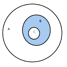
Figure 2: Example of disconnected background. Here $D_{0}=A\cup C$ and $D_{1}=B$ is a low-conductivity inclusion. See Remark 13.

When $D_{0}$ is not connected, the following observation can be made.

Remark 13

In the case of $D_{0}$ being disconnected, we have that (54) implies that $u_{-1}$ is constant in each connected component of $D_{0}$ and it vanishes only in the connected components whose boundary intersects $\partial D$. The function $u_{-1}$ will be constant in the other interior connected components. This is similar to the case of high-conductivity inclusions. The function $u_{-1}$ will be zero only if the forcing term vanishes in these interior components also; see Equations (20) and (49). For instance, consider the case illustrated in Figure 2 where the background domain are $D_{0}=A\cup C$ and the inclusions is given by $D_{1}=B$. In this case it is easy to see that $u_{-1}$ satisfies a problem similar to problem (14) in $B\cup\overline{C}$. Then, $u_{-1}$ will vanish only if the forcing term vanishes in $B\cup\overline{C}$. In this case, a result similar to Corollary 12 above can be stated.

5.3 Multiple low-conductivity inclusions

Let $\kappa$ be defined by

$$\kappa(x)=\left\{\begin{array}[]{cc}\epsilon&x\in D_{m},~{}~{}m=1,\dots,M,\\ 1,&x\in D_{0}=D\setminus\cup_{m=1}^{M}\overline{D}_{m},\end{array}\right.$$ (64)

and denote by $u_{\epsilon}$ the solution of (4) with coefficient (64). We assume that $D_{i}$ is compactly included in the open set $D\setminus\cup_{\ell=1,\ell\not=m}^{M}\overline{D}_{\ell}$, i.e., $\overline{D}_{m}\subset D\setminus\cup_{\ell=1,\ell\not=m}^{M}\overline{D}_{\ell}$, and we define $D_{0}:=D\setminus\cup_{m=1}^{M}\overline{D}_{m}$.

Expansion (52)-(53) extends easily to this case of multiple low-conductivity inclusions, that is,

• We have $u_{-1}^{(0)}=0$ on $D_{0}$. Also, that each, $u_{-1}^{(\ell)}$ satisfies the following Dirichlet problem in $D_{\ell}$,

  $$\begin{array}[]{c}\int_{D_{\ell}}\nabla u_{-1}^{(\ell)}\cdot\nabla z=\int_{D_{\ell}}fz\quad\mbox{ for all }z\in H^{1}_{0}(D_{\ell})\\ \\ u_{-1}^{(\ell)}=0\quad\mbox{ on }\partial D_{\ell}.\end{array}$$ (65)

• We can obtain $u_{0}^{(0)}$ in $D_{0}$ by solving the problem

  $$\begin{array}[]{c}\displaystyle\int_{D_{0}}\nabla u_{0}^{(0)}\cdot\nabla z=\int_{D_{0}}fz-\sum_{\ell=1}^{M}\int_{\partial D_{\ell}}\nabla u_{-1}^{(\ell)}\cdot n_{1}z\quad\forall z\in H^{1}(D_{0}),z|_{\partial D}=0,\\ \\ u_{0}^{(0)}=g\mbox{ on }\partial D.\end{array}$$ (66)

• Finally, we have that $u_{i}^{(\ell)}$ is harmonic in $D_{\ell}$ for all $i\geq 0$ and that $u_{i}^{(0)}$ is harmonic in $D_{0}$ for $i\geq 1$.

  Given $u_{i-1}^{(0)}$ in $D_{0}$, we can find $u_{i-1}^{(\ell)}$ in $D_{\ell}$ by solving the following Dirichlet problem with the known Dirichlet data,

  $$\begin{array}[]{c}\displaystyle\int_{D_{\ell}}\nabla u_{i-1}^{(\ell)}\cdot\nabla z=0\mbox{ for all }z\in H^{1}_{0}(D_{\ell})\\ u_{i-1}^{(\ell)}=u_{i-1}^{(0)}\mbox{ on }\partial D_{\ell}.\end{array}$$ (67)

  To find $u_{i}^{(0)}$ in $D_{0}$ we solve the problem

  $$\begin{array}[]{c}\displaystyle\int_{D_{0}}\nabla u_{i}^{(0)}\cdot\nabla z=-\sum_{\ell=1}^{M}\int_{\partial D_{\ell}}\nabla u_{i-1}^{(\ell)}\cdot n_{\ell}z\quad\forall z\in H^{1}_{0}(D_{0})\mbox{ with }z|_{\partial D}=0,\\ \\ u_{i}=0\mbox{ on }\partial D\subset\partial D_{0}.\end{array}$$ (68)

The convergence of the expansion (52)-(53) is similar to the case of one low-conductivity inclusion. In particular Corollary 11 holds in this case.

6 An example with low- and high- conductivity inclusions

In this section we show an example with a high- and a low-conductivity inclusion. The procedures were introduced in detail in Sections 4 and 5. We show only how to write the subdomains problems for the leading terms of the expansion.

Consider $\kappa$ to be defined by

$$\kappa(x)=\left\{\begin{array}[]{cc}\eta,&x\in D_{1},\\ {1}/{\eta},&x\in D_{2},\\ 1,&x\in D_{0}=D\setminus(\overline{D}_{1}\cup\overline{D}_{2}).\end{array}\right.$$ (69)

As before we write $u_{\eta}=\eta u_{-1}+u_{0}+\frac{1}{\eta}u_{1}+\frac{1}{\eta^{2}}u_{2}+\dots=\sum_{i=-1}^{\infty}\eta^{-i}u_{i},$ with $u_{0}=g$ on $\partial D$ and $u_{i}=0$ on $\partial D$ for $i\not=0$. We need that

$$\eta^{2}\int_{D_{1}}\nabla u_{-1}\cdot\nabla v+\eta\left(\int_{D_{0}}\nabla u_{-1}\cdot\nabla v+\int_{D_{1}}\nabla u_{0}\cdot\nabla v\right)+$$

$$\quad\sum_{i=0}^{\infty}\eta^{i}\left(\int_{D_{0}}\nabla u_{i}\cdot\nabla v+\int_{D_{1}}\nabla u_{i+1}\cdot\nabla v+\int_{D_{2}}\nabla u_{i-1}\cdot\nabla v\right)=\int_{D}fv.$$

Now we equate powers and analyze the subdomain equations. We assume that $D_{i}$ is connected and compactly included in $D$ ($\overline{D}_{i}\subset D$), $i=1,2$. We also assume that the distance between $D_{1}$ and $D_{2}$ is strictly positive, then $u_{-1}^{(0)}=0$, $u_{-1}^{(1)}=0$ and $u_{-1}^{(2)}$ solves the following Dirichlet problem in $D_{1}$,

$$\begin{array}[]{c}\int_{D_{1}}\nabla u_{-1}^{(2)}\cdot\nabla z=\int_{D_{1}}fz\quad\mbox{ for all }z\in H^{1}_{0}(D_{1})\\ \\ u_{-1}^{(2)}=0\mbox{ on }\partial D_{1}.\end{array}$$ (70)

This defines the function $u_{-1}$. To write a problem for $u_{0}$, let

$$V_{const}=\{v\in H^{1}(D\setminus\overline{D}_{2}),\mbox{ such that }v=0\mbox{ on }\partial D\mbox{ and }v^{(1)}=v|_{D_{1}}\mbox{ is constant }\}.$$

We have that

$$\begin{array}[]{c}\int_{D_{0}}\nabla u_{0}\cdot\nabla z=\int_{D}fz-\int_{\partial D_{2}}\nabla u_{-1}^{(2)}\cdot n_{2}z\mbox{ for all }z\in V_{const},\\ \\ u_{0}=g\mbox{ on }\partial D.\end{array}$$ (71)

The problem above can be analyzed using the harmonic characteristic function $\chi_{D_{1}}\in H^{1}_{0}(D)$ defined in (38) with $M=2$. The solution of the asymptotic problem above gives $u_{0}^{(0)}$ and the constant function $u_{0}^{(1)}$. As before, the constant $u_{0}^{(1)}$ can be determined explicitly using an expression similar to (21). To complete the definition of $u_{0}$ we observe that $u_{0}^{(2)}$ satisfies the following Dirichlet problem with the known Dirichlet data,

$$\begin{array}[]{c}\int_{D_{2}}\nabla u_{0}^{(2)}\cdot\nabla z=0\mbox{ for all }z\in H^{1}_{0}(D_{1})\\ \\ u_{0}^{(2)}=u_{0}^{(0)}\mbox{ on }\partial D_{1}.\end{array}$$ (72)

The functions $u_{i}$, $i=1,\dots$, can be determined form the equation

$$\int_{D_{0}}\nabla u_{i}\cdot\nabla v+\int_{D_{1}}\nabla u_{i+1}\cdot\nabla v+\int_{D_{2}}\nabla u_{i-1}\cdot\nabla v=0\quad\mbox{ for all }v\in H^{1}_{0}(D).$$

This procedure is similar to the ones developed before and presented in detail in Sections 4 and 5. As before, $u_{i}$ is harmonic in each region. Its restriction to subregions can be determined by solving subdomain problems involving Dirichlet, Neumann or mixed boundary conditions on the inclusions boundaries.

7 Conclusions and comments

We use asymptotic expansions to study high-contrast problems. We derive and analyze asymptotic power series for high-contrast elliptic problems. We mostly consider the case of binary media with interior isolated inclusions. High- or low-conductivity inclusion configurations are considered. The coefficients in the expansions are determined sequentially by a Dirichlet-to-Neumann procedure. In the case of high-conductivity inclusions, the Neumann problem needs to satisfy a compatibility of fluxes. This flux-compatibility condition is obtained using an auxiliary finite dimensional projection problem. The related finite dimensional space is spanned by harmonic extension of characteristic functions of each subdomain.

The asymptotic limits when the contrast increases to infinity are recovered and analyzed; see Theorems 5 and 8 and Corollary 12. The convergence of the expansions in $H^{1}(D)$ is obtained provided that the contrast is larger than a constant $C$ that depends on the background domains and the domains representing the inclusions. The convergence rate is algebraic. We consider the case of isolated interior inclusions which can be high and low conductivities. Other more complex configurations can be analyzed following a similar procedure. The analysis covers the cases with high- and low-conductivity inclusions. See Figure 3 for schematic representations of two dimensional configurations. If the low-conductivity value is $\epsilon$ and the high-conductivity value is $\eta=1/\epsilon$, then, an expansion similar to (52)-(53) can be used for all the examples in Figure 3. For general values of $\eta(\epsilon)=\epsilon^{-\rho}$, an expansion similar to (52)-(53) can also be derived where the coefficients in front of spatial terms will scale as $\epsilon^{l+m\rho}$, where $l\geq-1$ and $m\geq 0$ are integers.

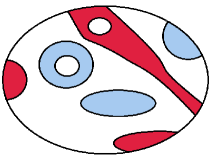
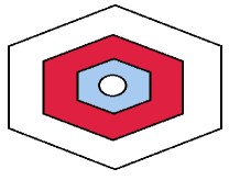
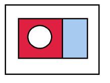
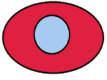
Figure 3: Four different configurations with high-conductivity $1/\epsilon$ (red) and low-conductivity $\epsilon$ (blue) regions. Expansion (52) can be obtained in these cases.

More general coefficients can also be studied. Similar expansions for other problems related with flows in high-contrast multiscale media can be obtained, e.g., models like heat conduction, wave propagation, Darcy or Brinkman flow, and elasticity problems. Efficient solution techniques for solving the system of linear equations (41) will be a subject of future research, in particular, localization procedures for the harmonic characteristic functions will be studied. Questions concerning the convergence of the series in stronger norms as well as computing quantities of interest will be studied in the future. Reduced contrast approximation and related multiscale methods as in [13, 12] will be the subject of future studies.

References

- [1] J. Aarnes and T. Hou, Multiscale domain decomposition methods for elliptic problems with high aspect ratios, Acta Math. Appl. Sin. Engl. Ser., 18(1):63-76, 2002.
- [2] I. Babuška and R. Lipton, Optimal Local approximation spaces for generalized finite element methods with application to multiscale problems, submitted.
- [3] A. Bensoussan, J. L. Lions, and G. Papanicolaou, Asymptotic analysis for periodic structures, Volume 5 of Studies in Mathematics and Its Applications, North-Holland Publ., 1978.
- [4] L. Berlyand and A. Novikov, Error of the network approximation for densely packed composites with irregular geometry, SIAM Journal on Mathematical Analysis, 34(2) (2002). 385-408.
- [5] Berlyand, Leonid; Cardone, Giuseppe; Gorb, Yuliya; Panasenko, Gregory. Asymptotic analysis of an array of closely spaced absolutely conductive inclusions. Netw. Heterog. Media 1 (2006), no. 3, 353–377. MR2247782 (2007m:35008) Add to clipboard
- [6] Berlyand, Leonid; Gorb, Yuliya; Novikov, Alexei. Discrete network approximation for highly-packed composites with irregular geometry in three dimensions. Multiscale methods in science and engineering, 21–57, Lect. Notes Comput. Sci. Eng., 44, Springer, Berlin, 2005.
- [7] L. Berlyand and H. Owhadi, A new approach to homogenization with arbitrary rough high contrast coefficients for scalar and vectorial problems, submitted.
- [8] L. Berlyand and H. Owhadi, Flux norm approach to finite dimensional homogenization approximations with non-separated scales and high contrast, Archives for Rational Mechanics and Analysis (2010, Volume 198, Number 2, 677-721).
- [9] L. Borcea and G.C. Papanicolaou, Network approximation for transport properties of high contrast materials, SIAM Journal on Applied Mathematics, vol. 58, no. 2, 1998, 501-539.
- [10] V. M. Calo, Y. Efendiev, and J. Galvis, A note on vatiational multiscale methods for high-contrast heterogeneous flows with rough source terms, 34 (9), September 2011, pp. 1177-1185.
- [11] T. Chartier, R. Falgout, V.E. Henson, J. Jones, T. Manteuffel, S. McCormick, J. Ruge, and P.S. Vassilevski, Spectral element agglomerate AMGe, in Domain Decomposition Methods in Science and Engineering XVI, Lecture Notes in Computational Science and Engineering, Springer-Verlag, Berlin Heidelberg 55(2007), 515-524.
- [12] C.C. Chu, I.G. Graham, and T.Y. Hou, A new multiscale finite element method for high-contrast elliptic interface problem, Math. Comp., 79 , 1915-1955, 2010.
- [13] E. Chung and Y. Efendiev, Reduced-contrast approximations for high-contrast multiscale flow problems, Multiscale Model. Simul. 8 (2010), no. 4, pp. 1128-1153.
- [14] Dang Quang A. Approximate method for solving an elliptic problem with discontinuous coefficients. J. Comput. Appl. Math. 51 (1994), no. 2, 193–203.
- [15] M. Dryja, Multilevel Methods for Elliptic Problems with Discontinuous Coefficients in Three Dimensions, Seventh International Conference of Domain Decomposition Methods in Scientific and Engineering Computing, by David E. Keyes and Jinchao Xu, vol. 180, 1994, 43-47.
- [16] Y. Efendiev and J. Galvis, A domain decomposition preconditioner for multiscale high-contrast problems, in Domain Decomposition Methods in Science and Engineering XIX, Huang, Y.; Kornhuber, R.; Widlund, O.; Xu, J. (Eds.), Volume 78 of Lecture Notes in Computational Science and Engineering, Springer-Verlag, 2011, Part 2, 189-196.
- [17] Y. Efendiev, J. Galvis and P. Vassielvski, Spectral element agglomerate algebraic multigrid methods for elliptic problems with high-Contrast coefficients, in Domain Decomposition Methods in Science and Engineering XIX, Huang, Y.; Kornhuber, R.; Widlund, O.; Xu, J. (Eds.), Volume 78 of Lecture Notes in Computational Science and Engineering, Springer-Verlag, 2011, Part 3, 407-414.
- [18] Y. Efendiev, J. Galvis, R. Lazarov and J. Willems, Robust domain decomposition preconditioners for abstract symmetric positive definite bilinear forms, submitted.
- [19] Y. Efendiev, J. Galvis, and X. H. Wu, Multiscale finite element methods for high-contrast problems using local spectral basis functions, Journal of Computational Physics. Volume 230, Issue 4, 20 February 2011, Pages 937-955.
- [20] Y. Efendiev and T. Hou, Multiscale finite element methods. Theory and applications, Springer, 2009.
- [21] R.E. Ewing, O. Iliev, R.D. Lazarov, I. Rybak, and J. Willems. A simplified method for upscaling composite materials with high contrast of the conductivity. SIAM Journal on Scientific Computing, 31(4):2568–2586, 2009.
- [22] J. Galvis and Y. Efendiev, Domain decomposition preconditioners for multiscale flows in high contrast media, SIAM MMS, Volume 8, Issue 4, 1461-1483 (2010).
- [23] J. Galvis and Y. Efendiev, Domain decomposition preconditioners for multiscale flows in high-contrast media: Reduced dimension coarse spaces, SIAM MMS, Volume 8, Issue 5, 1621-1644 (2010).
- [24] I. G. Graham, P. O. Lechner, and R. Scheichl, Domain decomposition for multiscale PDEs, Numer. Math., 106(4):589-626, 2007.
- [25] Grisvard, P. Elliptic problems in nonsmooth domains. Monographs and Studies in Mathematics, 24. Pitman (Advanced Publishing Program), Boston, MA, 1985.
- [26] T.Y. Hou and X.H. Wu, A multiscale finite element method for elliptic problems in composite materials and porous media, Journal of Computational Physics, 134 (1997), 169-189.
- [27] Klapper, I.; Shaw, T. A large jump asymptotic framework for solving elliptic and parabolic equations with interfaces and strong coefficient discontinuities. Appl. Numer. Math. 57 (2007), no. 5-7, 657–671
- [28] T. P. A. Mathew, Domain decomposition methods for the numerical solution of partial differential equations, volume 61 of Lecture Notes in Computational Science and Engineering, Springer-Verlag, Berlin, 2008.
- [29] F. Nataf, H. Xiang, V. Dolean, N. Spillane, A coarse space construction based on local Dirichlet to Neumann maps, accepted for publication in SIAM J. Sci Comput., 2011.
- [30] S.V. Nepomnyaschikh, Mesh theorems on traces, normalizations of function traces and their inversion, Soviet J. Numer. Anal. Math. Modelling, 6(2):151-168, 1991.
- [31] H. Owhadi and L. Zhang, Localized bases for finite dimensional homogenization approximations with non-separated scales and high-contrast, submitted to SIAM MMS, Available at Caltech ACM Tech Report No 2010-04. arXiv:1011.0986
- [32] Pavliotis, Grigorios A.; Stuart, Andrew M. Multiscale methods. Averaging and homogenization. Texts in Applied Mathematics, 53. Springer, New York, 2008.
- [33] C. Pechstein and R. Scheichl, Analysis of FETI methods for multiscale PDEs, Numerische Mathematik 111(2):293-333, 2008.
- [34] M. Sarkis, Nonstandard coarse spaces and Schwarz methods for elliptic problems with discontinuous coefficients using non-conforming elements, Numer. Math., 77(3), 383-406, 1997.
- [35] A. Toselli and O. Widlund. Domain decomposition methods—algorithms and theory, volume 34 of Springer Series in Computational Mathematics, Springer-Verlag, Berlin, 2005.
- [36] J. Van lent, R. Scheichl, and I.G. Graham, Energy-minimizing coarse spaces for two-level Schwarz methods for multiscale PDEs. Numer. Linear Algebra Appl. 16 (2009), no. 10, 775-799.
- [37] P.S. Vassilevski, ”Coarse Spaces by Algebraic Multigrid: Multigrid Convergence and Upscaling Error Estimates, (2010) (to appear). Available as Lawrence Livermore National Laboratory Technical Report LLNL-PROC-432896, May 21, 2010.
- [38] J. Xu and L. Zikatanov, On an energy minimizing basis for algebraic multigrid methods, Comput. Visual Sci., 7:121-127, 2004.