Large collection of astrophysical S-factors and its compact representation

Abstract

Numerous nuclear reactions in the crust of accreting neutron stars are strongly affected by dense plasma environment. Simulations of superbursts, deep crustal heating and other nuclear burning phenomena in neutron stars require astrophysical $S$-factors for these reactions (as a function of center-of-mass energy $E$ of colliding nuclei). A large database of $S$-factors is created for about 5,000 non-resonant fusion reactions involving stable and unstable isotopes of Be, B, C, N, O, F, Ne, Na, Mg, and Si. It extends the previous database of about 1,000 reactions involving isotopes of C, O, Ne, and Mg. The calculations are performed using the São Paulo potential and the barrier penetration formalism. All calculated $S$-data are parameterized by an analytic model for $S(E)$ proposed before [Phys. Rev. C 82, 044609 (2010)] and further elaborated here. For a given reaction, the present $S(E)$-model contains three parameters. These parameters are easily interpolated along reactions involving isotopes of the same elements with only seven input parameters, giving an ultracompact, accurate, simple, and uniform database. The $S(E)$ approximation can also be used to estimate theoretical uncertainties of $S(E)$ and nuclear reaction rates in dense matter, as illustrated for the case of the ³⁴Ne+³⁴Ne reaction in the inner crust of an accreting neutron star.

I Introduction

Nuclear burning is an important ingredient of stellar structure and evolution bbfh57 ; fh64 ; clayton83 . Simulating the evolution and observational manifestations of different stars (from main-sequence, to giants and supergiants, presupernovae, white dwarfs and neutron stars), requires the rates of many reactions, involving different nuclei – light and heavy, stable and neutron-rich. These rates are derived from respective reaction cross sections $\sigma(E)$, where $E$ is the center-of-mass energy of reactants.

The rates of many reactions which occur in the classical thermonuclear regime – for instance, in main-sequence stars – are well known. However nuclear burning in dense plasma of white dwarfs and neutron stars st83 , which affects the evolution and many observational manifestations of these objects, may proceed in other regimes, under strong effects of plasma screening and pycnonuclear tunneling through Coulomb barrier (e.g., Refs. svh69 ; yak2006 ; cd09 ). The burning powers nuclear explosions in surface layers of accreting white dwarfs (nova events), in cores of massive accreting white dwarfs or in binary white dwarf mergers (type Ia supernovae) NiWo97 ; hoeflich06 ; vankerkwijketal2010 , and in surface layers of accreting neutron stars (type I X-ray bursts and superbursts; e.g., Refs. sb06 ; schatz03 ; cummingetal05 ; Brown06 ; cooperetal09 ). Nova events and type I X-ray bursts are mostly driven by the proton capture reactions of the hot CNO cycles and by the rp-process. This burning is thermonuclear, without any strong effects of dense plasma environment. Type Ia supernovae and superbursts are driven by the burning of carbon, oxygen, and heavier elements at high densities, where the plasma screening effects can be substantial. It is likely that pycnonuclear burning of neutron-rich nuclei (e.g., ³⁴Ne+³⁴Ne) in the inner crust of accreting neutron stars in X-ray transients (in binaries with low-mass companions; e.g. Refs. hz90 ; hz03 ; Brown06 ) provides an internal heat source for these stars. If so, it powers Brown98 thermal surface X-ray emission of neutron stars observed in quiescent states of X-ray transients (see, e.g., Refs. Brown06 ; pgw06 ; lh07 ) although other energy sources can also be important there (e.g., Ref. bk09 ).

Therefore, in dense plasma of evolved stars, standard classical thermonuclear reaction rates may be unavailable and/or inapplicable. Accordingly, one needs to construct many reaction rates, valid over all burning regimes, starting from reaction cross sections $\sigma(E)$. Here we focus on non-resonant fusion reactions involving $(A_{1},Z_{1})$ and $(A_{2},Z_{2})$ reactants ($A_{i}$ and $Z_{i}$ stand for their mass and charge numbers), which may occur in evolved stars. The cross section $\sigma(E)$ is conveniently expressed through the astrophysical $S$-factor,

$$\sigma(E)=E^{-1}\,\exp(-2\pi\eta)\,S(E),$$ (1)

where $\eta=\alpha/(\hbar v)=\sqrt{E_{R}/E}$ is the Sommerfeld parameter, $v=\sqrt{2E/\mu}$ is the relative velocity of the reactants at large separations, $\alpha=Z_{1}Z_{2}e^{2}$, $E_{R}=\alpha^{2}\mu/(2\hbar^{2})$ is analogous to the Rydberg energy in atomic physics, and $\mu$ is the reduced mass. The factor $\exp(-2\pi\eta)$ is proportional to the probability of penetration through the pure Coulomb barrier $U(r)=\alpha/r$ with zero angular orbital momentum, assuming that this pure Coulomb barrier extends to $r\to 0$ (as for point-like nuclei); $E^{-1}$ factorizes out the well-known pre-exponential low-energy dependence of $\sigma(E)$. The advantage of this representation is that $S(E)$ is a more slowly varying function of $E$ than $\sigma(E)$.

For astrophysical applications, one needs $S(E)$ at low energies, $E\lesssim$ a few MeV. Even for beta-stable nuclei experimental measurements of $\sigma(E)$ at such energies are mainly not available because the Coulomb barrier becomes extremely thick making $\sigma(E)$ exponentially small. It will be even more difficult to get such data for neutron-rich nuclei. Moreover, the modelling of the processes at different astrophysical sites (such as dynamic reaction network modeling of the neutron star crust composition at high densities MW-08 ) requires the knowledge of $S$-factors for a large variety of reactions, many of which involve neutron-rich nuclei. The experimental study of so many reactions is definitely beyond existing and near-future capabilities. Therefore, one must rely on theoretical calculations.

Previously paper1 we calculated $S(E)$ for 946 reactions involving isotopes of C, O, Ne, and Mg. Also, we proposed paper2 a simple analytic model for $S(E)$ and used it to fit calculated $S$-factors. The present paper significantly enlarges the database. We have extended the calculations to incorporate new reactions between even-even and odd($Z$)-even isotopes. In particular, we have calculated $S(E)$ between isotopes of  Be, B, C, N, O, F, Ne, Na, Mg, and Si. Our new database of $S(E)$ contains 4,851 reactions. Moreover, we elaborate and simplify the analytic $S(E)$-model, and use it to parameterize all $S$-factors with the minimum number of fit parameters producing thus an ultracompact and uniform database convenient in applications.

II Calculations

Consider a set of $S$-factors for non-resonant fusion reactions involving various isotopes of 10 elements, Be, B, C, N, O, F, Ne, Na, Mg, and Si. The $S$-factors for the reactions involving even-even isotopes of C, O, Ne, and Mg have been calculated recently in our previous paper paper1 . Calculations for other reactions are original and include even-even and odd($Z$)-even stable, proton-rich, neutron-rich, and very neutron-rich isotopes. Such isotopes can appear during nuclear burning in stellar matter, particularly, in the cores of white dwarfs and envelopes of neutron stars. The calculations have been performed using the São Paulo potential in the frame of the barrier penetration model gas2005 . Nuclear densities of reactants have been obtained in Relativitic Hartree-Bogoliubov (RHB) theory VALR.05 employing the NL3 parametrization for relativistic mean field Lagrangian NL3 and Gogny D1S force for pairing. The model is based on the standard partial wave decomposition ($\ell=0,1,\ldots$) and considers the motion of reacting nuclei in the effective potential discussed in Sec. III.3 [see Eq. (10) there]. The numerical scheme is parameter-free and relatively simple for generating a set of data for many non-resonant reactions involving different isotopes.

The reactions in question are listed in Table 1. All reactants are either even-even or odd-even nuclei. We consider 55 reaction types, such as Si+Si and Be+B, with the range of mass numbers for both species given in the columns 2 and 3 of Table 1. For each reaction, $S(E)$ has been computed on a dense grid of $E$ (with the energy step of 0.1 MeV) from 2 MeV to a maximum value $E_{\mathrm{max}}$ (also given in Table 1) covering wide energy ranges below and above the Coulomb barrier. The last column in Table 1 presents the number of considered reactions.

$S(E)$-factors calculated using the São Paulo potential have been compared previously yak2006 ; gas2005 ; saoPauloTool with experimental data and with theoretical calculations performed using other models such as coupled-channels and fermionic molecular dynamics ones. Let us stress that the calculated values of $S(E)$ are uncertain due to nuclear physics effects – due to using the São Paulo model with the NL3 nucleon density distribution. As shown, for instance, in Ref. saoPauloTool , typical expected uncertainties for the reactions involving stable nuclides are within a factor of 2, with maximum up to a factor of 4. For the reactions involving unstable nuclei, typical uncertainties can be as large as one order of magnitude, reaching two orders of magnitude at low energies for the reactions with very neutron-rich isotopes. These uncertainties reflect the current state of the art in our knowledge of $S(E)$.

III Analytic model

III.1 General remarks

Let us recall the main features of the analytic model for $S(E)$ proposed in Ref. paper2 and used there to fit the initial set of 946 $S$-factors. We will elaborate and simplify the model, and fit much larger set of data.

The model paper2 is based on semi-classical consideration of quantum tunneling through an effective potential $U(r)$ (which is purely Coulombic at large separations $r$ but is truncated by nuclear interactions at small $r$ when colliding nuclei merge). The reaction cross section at $E<E_{C}$ (where $E_{C}$ is the barrier height) is taken in the form

$$\sigma(E) = \frac{S_{0}}{E}\exp\left[-{2\over\hbar}\int_{r_{1}}^{r_{2}}{\rm d}r\,\sqrt{2\mu(U-E)}\right],$$ (2)

where $r_{1}$ and $r_{2}$ are classical turning points; $S_{0}$ is a slowly varying function of $E$ treated as a constant; it has the same dimension as $S(E)$, but should not be confused with it.

To obtain tractable formulae for $S(E)$, in Ref. paper2 we employed the natural and simplest approximation of $U(r)$,

$$U(r)={\alpha\over r}~{}~{}~{}\mathrm{at}~{}~{}r\geq R_{C1},$$

$$U(r)=E_{C}\left[1-\beta{(r-R_{C})^{2}\over R_{C}^{2}}\right]~{}~{}~{}\mathrm{at}~{}~{}r<R_{C1},$$ (3)

which is a pure Coulomb potential at $r\geq R_{C1}$ and an inverse parabolic potential at smaller $r$ (see Fig. 1 in Ref. paper2 ). The parabolic segment truncates the effective interaction at small separations; $E_{C}=U(R_{C})$ is the maximum of $U(r)$, that is the barrier height. We required $U(r)$ and its derivative to be continuous at $r=R_{C1}$. Instead of $\beta$ we will often use $\delta=(R_{C1}-R_{C})/R_{C}$, which characterizes the width of the peak maximum of $U(r)$. Then $U(r)$ is specified by two parameters, $E_{C}$ and $\delta$, with paper2

$$R_{C}={\alpha(2+3\delta)\over 2E_{C}(1+\delta)^{2}},\quad\beta={1\over\delta(2+3\delta)},$$

$$R_{C1}=R_{C}\,(1+\delta),\quad E_{C1}=U(R_{C1})=E_{C}\,{2+2\delta\over 2+3\delta}.$$ (4)

The potential $U(r)$ passes through zero at $r=R_{C0}=R_{C}(1-\beta^{-1/2})$; its behavior at smaller $r$ is unimportant (in our approximation). Realistic models should correspond to $\beta\gg 1$ (the small-$r$ slope of $U(r)$ should be sharp; $R_{C0}$ should be positive) which translates into $\delta\ll{1\over 3}$ (because $\beta=1$ corresponds to $\delta={1\over 3}$).

III.2 Sub-barrier energies

With the potential (3) at $E<E_{C}$ one has

$$S(E)=S_{0}\,\exp\Psi(E),$$ (5)

where $\Psi(E)$ is taken analytically and has a rather complicated form given by Eq. (9) in Ref. paper2 . Notice that in our semi-classical approximation $\Psi(E_{C})=2\pi\eta_{C}$, where $\eta_{C}=\eta(E_{C})$ is the Sommerfeld parameter at $E=E_{C}$.

In this paper we propose a simplified expression for $S(E)$ at $E<E_{C}$. Let us recall that $\Psi(E)$ at $E<E_{C}$ is accurately approximated paper2 by the Taylor expansion $\Psi(E)=g_{0}+g_{1}E+g_{2}E^{2}+\ldots$ The explicit expressions for the expansion coefficients $g_{0}$, $g_{1}$, and $g_{2}$ in terms of $E_{C}$ and $\delta$ are given by Eqs. (14) and (15) of Ref. paper2 . At $E<E_{C}$ we suggest the approximation

$$\Psi(E)=g_{0}+g_{1}E+g_{2}E^{2},$$ (6)

$$g_{2}=(2\pi\eta_{C}-g_{0}-g_{1}E_{C})/E_{C}^{2}.$$ (7)

The expressions for $g_{0}$ and $g_{1}$ will be taken from Ref. paper2 , while $g_{2}$ is introduced in such a way to satisfy the condition $\Psi(E_{C})=2\pi\eta_{C}$. Our polynomial approximation (6) is much simpler than the exact expression (9) of Ref. paper2 but gives nearly the same accuracy in approximating all $S(E)$-factors considered in Sec. II. Nevertheless, it is still not very convenient in applications because Eqs. (14) and (15) of Ref. paper2 for $g_{0}$ and $g_{1}$ are rather complicated. Therefore we further simplify these equations by adopting the limit of $\delta\ll 1$, which is sufficient for applications in Sec. IV. In this limit we have paper2

$$g_{0}=\sqrt{E_{R}\over E_{C}}\;(8-\pi\,\sqrt{2\delta}-2\delta),$$ (8)

$$g_{1}=-\sqrt{E_{R}\over E_{C}^{3}}\,\left({4\over 3}-\pi\sqrt{2\delta}-\delta\right).$$ (9)

Thus, Eqs. (5)–(9) give simple and practical expressions for $S(E)$ at $E<E_{C}$. In our model, $S(E)$ is determined by the three parameters, $E_{C}$, $\delta$, and $S_{0}$; $E_{C}$ and $\delta$ determine the shape of the potential $U(r)$; $S_{0}$ specifies the efficiency of fusion reaction.

III.3 Contribution of $\ell>0$ waves

The proposed model is phenomenological, being based on $s$-wave semi-classical tunneling through a spherical potential barrier $U(r)$. The actual reaction cross section $\sigma(E)$ contains contribution of different $\ell$ waves, with $\ell=0,1,2,\ldots$ For a given multipolarity $\ell$, we have a quantum mechanical scattering problem of two nuclei moving in an effective potential

$$V_{\mathrm{eff}}(r)=U(r)+V_{\ell}(r),\quad V_{\ell}(r)=\frac{\hbar^{2}\ell(\ell+1)}{2\mu r^{2}},$$ (10)

where $V_{\ell}(r)$ is the centrifugal potential. Then the cross section is (e.g., Refs. vas81 ; leandro04 )

$$\sigma(E)={\pi\over k^{2}}\,\sum_{\ell=0}^{\infty}(2\ell+1)T_{\ell}(E)\,P_{\ell}(E),$$ (11)

where $k$ is wave-number ($E=\hbar^{2}k^{2}/2\mu$), $T_{\ell}(E)$ is the transmission coefficient, and $P_{\ell}(E)$ is the fusion probability for the penetrating wave. At the low energies of our interest, one traditionally assumes $P_{\ell}(E)=1$.

Let us return to our $S(E)$-model at $E<E_{C}$. In accordance with (11), we have $S(E)=\sum_{\ell}S^{(\ell)}(E)$, where $S^{(\ell)}(E)$ is an $\ell$-wave contribution to $S(E)$ to be calculated using the effective potential $V_{\mathrm{eff}}(r)$. At $E<E_{C}$, all $\ell$ waves refer to subbarrier motion, and the transmission coefficient $T_{\ell}(E)$ decreases evidently with the growth of $\ell$. Then $S(E)$ can be written as

$$S(E)=S^{(0)}(E)\,J(E),\quad J(E)=1+\sum_{\ell=1}^{\infty}(2\ell+1){T_{\ell}(E)\over T_{0}(E)}.$$ (12)

Here, $S^{(0)}(E)$ is the $s$-wave contribution, and the sum in $J(E)$ is the correction due to waves with $\ell\geq 1$.

A simple analysis shows that $S(E)$ is typically determined by several lowest $\ell$ at $E<E_{C}$ for reactions considered in Sec. II. The correction factor $J(E)$ appears to be essentially higher than 1 (values $\ell>0$ are important) but is a slowly varying function of $E$. In other words, the transmission coefficients $T_{\ell}(E)$ at these $\ell$ are similar functions of $E$. Their main energy dependence is the same as for $s$-wave, $S^{(0)}(E)$. A crude estimate at $E$ noticeably below $E_{C}$ gives $J(E)\sim 1+\sqrt{E_{C}/E_{0}}$, where $E_{0}=\hbar^{2}/(2\mu R_{C}^{2})$ is the characteristic quantum of centrifugal energy (typically, $E_{0}\ll E_{C}$). To simplify the model, at $E<E_{C}$ we suggest the approximation

$$S(E) = S_{0s}J_{0}\,\exp(g_{0}+g_{1}E+g_{2}E^{2}),$$ (13)

$$J_{0} = 1+j_{0}\sqrt{E_{C}/E_{0}}.$$ (14)

Here, $S_{0s}$ is the $s$-wave contribution to $S_{0}$, $J(E)$ is approximated by energy-independent constant $J_{0}$ (that is specified by a constant $j_{0}$); $J_{0}$ (or $j_{0}$) can be treated as a parameter which characterizes the importance of higher multipolarities $\ell>0$. One often states in quantum mechanics that the main contribution to scattering at low $E$ comes from $\ell=0$. This statement does not apply to the potential considered here, which has strong attraction at $r=0$. In this case, higher $\ell$ are important even at very low $E$.

Finally, at $E=E_{C}$, the $s$-wave barrier is removed and we have $T_{0}(E_{C})=1$ in Eq. (11). Then the $s$-wave partial cross section is $\sigma_{0}(E_{C})=\pi/k_{C}^{2}$, where $k_{C}$ is the wave-number referring to $E=E_{C}$. From this $\sigma_{0}(E_{C})$ and Eq. (1) we immediately get:

$$S_{0s}={\pi\hbar^{2}\over 2\mu}=0.6566\,{A_{1}+A_{2}\over A_{1}A_{2}}~{}~{}\mathrm{MeV~{}barn}.$$ (15)

Therefore, $S_{0s}$ is specified by $A_{1}$ and $A_{2}$. The astrophysical $S$-factor at $E<E_{C}$ is determined by the parameters $E_{C}$ and $\beta$ (or $\delta$) of the $U(r)$ potential and by the factor $J_{0}$ (or $j_{0}$).

III.4 Above-barrier energies

At $E>E_{C}$ the effective barrier is transparent for some low-$\ell$ waves. In this case we adopt the simplest barrier-penetration model with $T_{\ell}(E)=1$ if the $V_{\mathrm{eff}}(r)$ barrier is transparent at a given $E$, and with $T_{\ell}(E)=0$ otherwise. The cross section is then given by Eq. (11) with $T_{\ell}=1$ and $P_{\ell}=1$, where the sum is taken from $\ell=0$ to some maximum $\ell_{0}(E)$ at which $V_{\mathrm{eff}}(r)$ becomes classically forbidden. To be transparent at lower $\ell$, the $V_{\mathrm{eff}}(r)$ potential should have a pocket (with a local minimum) and a barrier (with a local peak) at $r<R_{C}$; let $r=r_{0}<R_{C}$ be the peak point. It is well known that in this case at $E>E_{C}$ the cross section becomes (e.g., Ref. vas81 )

$$\sigma(E)={\pi\over k^{2}}\,(\ell_{0}(E)+1)^{2}.$$ (16)

With increasing $E$, the range of $\ell\leq\ell_{0}(E)$ widens. In the spirit of semi-classical approximation, at $E>E_{C}$ we can treat $\ell_{0}(E)$ as a continuous variable. As long as $E$ is not too much higher than $E_{C}$, the local peak point $r_{0}$ of $V_{\mathrm{eff}}(r)$ is close to $R_{C}$. To locate this peak, it is convenient to introduce $x=(R_{C}-r)/R_{C}$ instead of $r$ and linearize $V_{\ell}(r)$ in terms of $x$, keeping constant and linear terms. The peak occurs at $x=x_{0}=(\ell+1)\ell E_{0}/(E_{C}\beta)$ at which ${\rm d}V_{\mathrm{eff}}/{\rm d}x=0$. The peak height is $V_{\mathrm{eff}}(r_{0})=E_{C}+(\ell+1)\ell E_{0}+(\ell+1)^{2}\ell^{2}E_{0}^{2}/(E_{C}\beta)$. At a given $E$ the barrier becomes classically forbidden when $V_{\mathrm{eff}}(r_{0})=E$, which gives a quadratic equation for $(\ell_{0}+1)\ell_{0}$. Solving this equation, we have

$$(\ell_{0}+1)\ell_{0}=\frac{\sqrt{E_{C}^{2}\beta^{2}+4E_{C}\beta(E-E_{C})}-E_{C}\beta}{2E_{0}}.$$ (17)

Now we can easily find $\ell_{0}(E)$. Substituting it into Eq. (16) gives a closed expression for $\sigma(E)$ at $E>E_{C}$.

However, such a solution seems overcomplicated. It can be further simplified if we notice that at not too high $E$ we typically have $E-E_{C}\ll\beta E_{C}$ and expand the expression containing square root. This gives

$$y(E)\equiv(\ell_{0}+1)\ell_{0}=\frac{E-E_{C}}{E_{0}}\,\left(1-\frac{E-E_{C}}{\beta E_{C}}\right),$$ (18)

the second term in the parentheses being a small correction.

One has $\ell_{0}(E)\gg 1$ very soon after $E$ exceeds the barrier $E_{C}$; then $(\ell_{0}+1)\ell_{0}\approx\ell_{0}^{2}$. On the other hand, at $E=E_{C}$ in the adopted approximation we should have $\ell_{0}(E_{C})=0$ and $\sigma_{0}(E_{C})=\pi/k_{C}^{2}$. Naturally, our approximation of continuous $\ell_{0}(E)$ is inaccurate just near the threshold ($E\to E_{C}$), where $s$-wave nuclear collisions proceed above the threshold, while higher-$\ell$ collisions operate either in the subbarrier regime or in the transition regime (emerging from under respective barriers with growing $E$). It is a complicated task to describe accurately $\sigma(E)$ and $S(E)$ at $E\approx E_{C}$. In order to preserve the simplicity of our $S(E)$ model we propose writing the cross section $\sigma(E)$ at $E>E_{C}$ as

$$\sigma(E)={\pi\over k^{2}}\,\sqrt{y^{2}(E)+J_{0}^{2}},$$ (19)

where $y(E)$ is given by Eq. (18) and $J_{0}$ by Eq. (14). Then at $E=E_{C}$ this equation matches the cross section model proposed for subbarrier energies (Sec. III.2) while at $E-E_{C}\gtrsim J_{0}E_{0}$ it reproduces the semi-classical cross section (16).

Translating the cross section (19) into $S(E)$, at $E>E_{C}$ we finally have

$$S(E)=S_{0s}\,\exp(2\pi\eta)\,\sqrt{y^{2}(E)+J_{0}^{2}}.$$ (20)

At $E-E_{C}\gg J_{0}E_{0}$ the leading term in the astrophysical $S$-factor is $S(E)\approx S_{0s}\,\exp(2\pi\eta)\,(E-E_{C})/E_{0}$. In the previous work we described $S(E)$ by a phenomenological expression (Eq. (6) in Ref. paper2 ). It reproduces this leading term at $J_{0}E_{0}\ll E-E_{C}\ll E_{C}$ (see the term containing $\xi$ in Eq. (6) of Ref. paper2 ) but diverges from it at higher $E$. Although we do not intend to propose an accurate approximation of $S(E)$ at high energies (few barrier energies $E_{C}$ and higher), we remark that the phenomenological expression (6) for $S(E)$ at $E>E_{C}$ in Ref. paper2 is now replaced by Eq. (20) which reproduces the correct semi-classical behavior of $S(E)$ above the barrier. Our new expression (20) is self-sufficient, it contains no extra input parameters in addition to those introduced for describing $S(E)$ at $E<E_{C}$ in Sec. III.2.

III.5 How to calculate $S(E)$

For any fusion reaction, $S(E)$ is determined by three input parameters, $E_{C}$, $\beta$ (or $\delta$, see Eq. (4)) and $J_{0}$ (or $j_{0}$, see Eq. (14)). The first two parameters specify the shape of the effective potential $U(r)$, Eq. (3); $J_{0}$ (or $j_{0}$) takes into account the contribution of higher $\ell=1,2,\ldots$ to $S(E)$. At $E<E_{C}$ the astrophysical factor $S(E)$ is given by Eq. (13), and at $E\geq E_{C}$ it is given by (20). The factor $S_{0s}$ entering these equations is defined by (15). The parameters $g_{0}$, $g_{1}$, and $g_{2}$ in Eq. (13) are given by (8), (9), and (7).

By construction, our $S(E)$ model can be accurate at $E$ up to a few $E_{C}$. Although the model is generally based on first principles, it is phenomenological in a narrow energy range near the barrier ($|E-E_{C}|\lesssim J_{0}E_{0}$). Our current $S(E)$ model is simpler than its previous version paper2 and contains 3 input parameters instead of 4 in paper2 . We will see that the current model is more accurate than the previous one.

Let us stress that our new version implies $\delta\ll 1$ (actually, $\delta\lesssim 0.1$) meaning that the maximum of the effective potential $U(r)$ [see Eq. (3)] is rather sharp. For broader maximum ($0.1\lesssim\delta\leq 1/3$), it would be more appropriate to use the same Eq. (20) at $E\geq E_{C}$ but replace our Eq. (13) at $E<E_{C}$ by Eqs. (5) and (9) of Ref. paper2 , setting $S_{0}=S_{0s}J_{0}$ in (9). Although this would complicate the expression for $S(E)$ at $E<E_{C}$, the fit parameters would preserve their meaning.

IV Fits

Let us approximate all calculated $S(E)$ using the analytic model of Sec. III. In Ref. paper2 we approximated $S(E)$ for the 946 reactions involving C, O, Ne, and Mg isotopes with the first version of the model. That approximation is sufficiently accurate, but we approximate those data again together with the new data using the elaborated $S(E)$-model to obtain a uniform database with minimum number of input parameters.

We consider reactions of each type (each line in Table 1) separately, and apply the analytic model (13) and (20) to every reaction. In this manner we determine 3 fit parameters, $E_{C}$, $\delta$ and $j_{0}$, for every reaction. For instance, we have $3\times 120=360$ parameters for Si+Si reactions. However, we notice that we can set $\delta$ and $j_{0}$ constant for all reactions of a given type (for example, $\delta=0.0409$ and $j_{0}=2.8162$ for all Si+Si reactions) without greatly increasing the fit errors. Such constant $\delta$ and $j_{0}$ are given in Table 2. Notice that while $j_{0}$ is constant for a given reaction type, $J_{0}$ is given by the scaling relation (14) and differs from one reaction to another.

Still, we need to specify the barrier height $E_{C}$ for every reaction. Collecting the values of $E_{C}$ for all reactions of each type, we were able to fit them by the same analytic expression as in Ref. paper2 :

$$E_{C} = {\alpha/R_{12}},\quad R_{12}=R+\Delta R_{1}\,|A_{1}-A_{10}|+\Delta R_{2}\,|A_{2}-A_{20}|,$$ (21)

where $A_{10}=2Z_{1}$ and $A_{20}=2Z_{2}$ are mass numbers of most stable isotopes; $\Delta R_{1}=\Delta R_{1a}$ at $A_{1}\geq A_{10}$; $\Delta R_{1}=\Delta R_{1b}$ at $A_{1}<A_{10}$; $\Delta R_{2}=\Delta R_{2a}$ at $A_{2}\geq A_{20}$; $\Delta R_{2}=\Delta R_{2b}$ at $A_{2}<A_{20}$. This gives 5 new fit parameters $R$, $\Delta R_{1a}$, $\Delta R_{2a}$, $\Delta R_{1b}$, $\Delta R_{2b}$ (also given in Table 2) for each reaction type, and, hence, 7 parameters in total.

As in Ref. paper2 , our fit procedure is based on standard relative deviations of calculated (calc) and fitted (fit) $S(E)$-factors. The absolute value of such a deviation in a point $E$ is $\eta(E)=|1-S_{\mathrm{fit}}(E)/S_{\mathrm{calc}}(E)|$. Fitting has been done by minimizing root-mean-square (rms) deviation $\eta_{\mathrm{rms}}$ over all energy grid points for all reactions involved in a fit. Column 9 of Table 2 lists $\eta_{\mathrm{rms}}$ for all reactions of a given type over all energy grid points (e.g., over $120\times 379=45,480$ points for the Si+Si reactions). Column 10 presents the maximum absolute value of the relative standard deviations, $\eta_{\mathrm{max}}$, over all these reactions and points. Root-mean-square values $\eta_{\mathrm{rms}}$ are reasonably small; they vary from $\eta_{\mathrm{rms}}\approx 0.07$ for B+B, B+C, and B+N reactions to $\eta_{\mathrm{rms}}\approx 0.28$ for Si+Si reactions. Maximum relative deviations are larger, reaching $\eta_{\mathrm{max}}\approx 1.12$ for Si+Si. Such large values of $\eta_{\mathrm{max}}$ hide the proper maximum difference of $S_{\mathrm{fit}}(E)$ to $S_{\mathrm{calc}}(E)$ in a fit.

To visualize this difference, in column 11 we list the maximum value of the parameter $\widetilde{\eta}(E)$ that we define as $\widetilde{\eta}(E)=S_{\mathrm{fit}}(E)/S_{\mathrm{calc}}(E)-1$ for $S_{\mathrm{fit}}(E)>S_{\mathrm{calc}}(E)$ and as $\widetilde{\eta}(E)=S_{\mathrm{calc}}(E)/S_{\mathrm{fit}}(E)-1$ for $S_{\mathrm{fit}}(E)\leq S_{\mathrm{calc}}(E)$. Thus defined, we have $\widetilde{\eta}=\eta$ at $S_{\mathrm{fit}}>S_{\mathrm{calc}}$ but $\widetilde{\eta}>\eta$ at $S_{\mathrm{fit}}<S_{\mathrm{calc}}$. For $\eta\ll 1$ we always have $\widetilde{\eta}\approx\eta$, but for $\eta\gtrsim 1$ the value of $\widetilde{\eta}$ can be much larger than $\eta$. One can see that $\widetilde{\eta}_{\mathrm{max}}+1$ is the maximum value among ratios $S_{\mathrm{fit}}/S_{\mathrm{calc}}$ (at $S_{\mathrm{fit}}>S_{\mathrm{calc}}$) and $S_{\mathrm{calc}}/S_{\mathrm{fit}}$ (at $S_{\mathrm{fit}}\leq S_{\mathrm{calc}}$) in a fit sample. For our Si+Si reactions we have $\widetilde{\eta}_{\mathrm{max}}+1\approx 5.40$. This relatively large difference between $S_{\mathrm{calc}}$ and $S_{\mathrm{fit}}$ occurs at one energy point in one of the 120 Si+Si reactions. Specifically, it happens for the ⁴⁸Si+⁴⁸Si reaction (at $E=12.1$ MeV) which involves very neutron-rich nuclei. Although $\widetilde{\eta}_{\mathrm{max}}+1$ is quite large, our fits are still acceptable because the expected nuclear physics uncertainties associated with calculating $S(E)$ for such nuclei are larger (Sec. II). Notice that $\eta_{\mathrm{max}}$ and $\widetilde{\eta}_{\mathrm{max}}$ in Table 2 can occur for the same reactions and in the same energy points, and they can even coincide there. This happens, for instance, for B+N reactions ($\eta_{\mathrm{max}}=\widetilde{\eta}_{\mathrm{max}}=0.37$ for ¹¹B+¹³N at $E=6.1$ MeV). However, they can also occur for different reactions and at different $E$ (for instance, in case of Si+Si we have $\eta_{\mathrm{max}}=1.12$ for the ⁴⁰Si+⁴⁰Si reaction at $E=14.2$ MeV). We could have changed the fit algorithm and obtain somewhat smaller $\widetilde{\eta}_{\mathrm{max}}$ (for instance, by minimizing $\widetilde{\eta}_{\mathrm{rms}}$ instead of $\eta_{\mathrm{rms}}$) but it would give somewhat larger ${\eta}_{\mathrm{rms}}$.

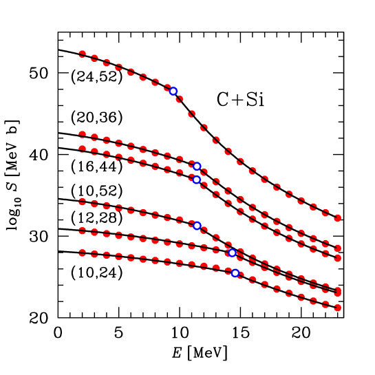
Figure 1: (Color online) $S$-factors for six C+Si reactions $A_{1}+A_{2}$ ($A_{1}$ and $A_{2}$ are given in parentheses). Filled dots are original calculations (on a rarefied grid of $E$ points); solid lines are our fits (Table 2); open dots show the fit values of $E_{C}$.

A graphical comparison of the previous fits with calculations for many reactions is presented in Figs. 3 and 4 of Ref. paper2 . The comparison with the new fits looks the same. For instance, in Fig. 1 we compare the fitted $S(E)$ (solid lines) with calculations (dots on a rarefied grid of $E$-points) for six C+Si reactions. The reactions are labeled by ($A_{1},A_{2}$), where $A_{1}$ and $A_{2}$ are mass numbers of C and Si isotopes, respectively. The lower line corresponds to the ¹⁰C+²⁴Si reaction involving the lightest (proton rich) nuclei from our collection (Table 1). The upper line is for the ²⁴C+⁵²Si reaction involving our most massive (neutron rich) C and Si isotopes. Other lines refer to intermediate cases, including the ¹²C+²⁸Si reaction of most stable nuclei. We see that the $S$-factors for C+Si reactions vary over many orders of magnitude but the fit accuracy remains acceptable.

The fit errors for the new $S(E)$-model are generally lower than for the previous one paper2 . For instance, for the O+O reactions we now have the maximum relative fit error $\eta_{\mathrm{max}}\approx 0.47$ and the rms relative fit error $\eta_{\mathrm{rms}}\approx 0.13$ while in Ref. paper2 we had $\eta_{\mathrm{max}}\approx 0.50$ and $\eta_{\mathrm{rms}}\approx 0.14$ (and we now have 7 fit parameters instead of 9). The fit accuracy is especially improved for reactions involving lower-$Z$ nuclei.

For some reaction types (e.g., for C+C), the fit errors of individual fits (made separately for every reaction) are noticeably lower than for all reactions of a given type. This indicates that the fit formula (21) for $E_{C}$ can be further improved. Also, we expect that the fit quality can be improved by introducing some slowly varying function $J(E)$ instead of constant $J_{0}$ at subbarrier energies in Eq. (14), and by elaborating the description of $S(E)$ at near-barrier energies $|E-E_{C}|\lesssim J_{0}E_{0}$. However, we think that the accuracy of the new fits is quite consistent with the quality of the present data (Sec. II). The fits give a compact and uniform description of calculated $S(E)$ for many reactions. They give reliable $S(E)$ in a wide range of energies $E$ because they are based on first principles. In addition, they are convenient for including into computer codes. We warn the readers that the calculated and fitted $S(E)$ do not take into account resonances. Therefore, one should add the resonance contribution in modeling nuclear burning which involves essentially resonant reactions.

Let us remark that our analytic model for $S(E)$ can also be used to reconstruct the interaction potential $U(r)$ by fitting the $S(E)$ data available from experiment or from calculations. Some examples have been presented in Ref. paper2 . Another example will be given below.

V Studying uncertainties of $S(E)$

This section illustrates another advantage of our analytic $S(E)$ model – its ability to study possible uncertainties of astrophysical reaction rates.

Clearly, any calculation of $S(E)$ contains some uncertainties. First of all, they can be associated with specific theoretical model. In our case (Sec. II) they are due to using the São Paulo potential, the barrier penetration model and the NL3 parametrization for deriving nuclear densities in the RHB theory. These uncertainties influence an effective potential $U(r)$ and, hence, $S(E)$. Fitting any given $S(E)$ with our model, one can estimate the effective potential $U(r)$ [find $\beta$ and $E_{C}$ in Eq. (3)]. Assuming reasonable uncertainties of $\beta$ and $E_{C}$ and using our $S(E)$-model again, one can easily estimate the expected range of $S(E)$ variations.

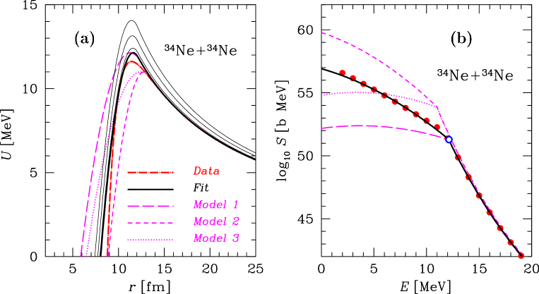
Figure 2: (Color online) Effective potentials $U(r)$ (left panel (a)) and respective astrophysical $S(E)$-factors (right panel (b)) for the ³⁴Ne+³⁴Ne reaction. The dot-dashed line on the left panel is the original São Paulo effective potential used in calculations (it slightly depends on $E$ and is taken at $E=10$ MeV); dots on the right panel are original calculated $S(E)$ on a rarefied grid of $E$-points. Thick solid lines show fitted $S(E)$ and $U(r)$ reconstructed from these fits. The three thin solid lines present appropriate effective potential $V_{\mathrm{eff}}(r)$ including the centrifugal term, Eq. (10), for $\ell$=5, 10, and 15 (from bottom to top). Long-dashed, short-dashed, and dotted lines refer to three models 1, 2, and 3, which illustrate possible effects of dense matter on the ³⁴Ne+³⁴Ne reaction (see text for details).

The $S(E)$-model can also be useful to estimate possible effects of dense matter. Consider, for instance, the heating of the inner crust of accreting neutron stars in X-ray transients (the so-called deep crustal heating hz90 ; hz03 ; Brown06 ). These transients are compact binary systems containing a neutron star and a low-mass companion. The deep crustal heating is thought to occur mainly due to pycnonuclear reactions in accreted matter when it sinks in the inner crust under the weight of newly accreted material. The heating can power Brown98 thermal surface emission of these neutron stars that is observed in quiescent states of transients (see, e.g., Refs. Brown06 ; lh07 ). Pycnonuclear reactions occur due to zero-point vibrations of atomic nuclei in a crystalline lattice. Their physics is described, for instance, by Salpeter and Van Horn svh69 and applied in later work (e.g. gas2005 ; yak2006 ; cdi07 ; cd09 and references therein). Pycnonuclear reactions occur at high densities and involve very neutron-rich nuclei hz90 ; hz03 , immersed in a sea of free neutrons available in the inner crust. For example, consider the powerful ³⁴Ne+³⁴Ne$\to^{68}$Ca reaction at $\rho\approx 1.7\times 10^{12}$ g cm^-3 in the scenario of Haensel and Zdunik hz90 . The fractional number of free neutrons among all nucleons in the burning layer is 0.39. The calculations of $S$-factors are performed for fusion of nuclei unaffected by dense fluid of free neutrons. However, such a fluid can compress the nuclei, modify their interaction potential $U(r)$, and hence $S(E)$.

Accurate calculations of $S(E)$ under these conditions have not been performed; they are complicated and do deserve a special study. Nevertheless, the $S(E)$-model allows us to estimate the range of expected $S(E)$ changes. This is illustrated in Fig. 2 which shows the model effective potentials (left panel (a)) and respective astrophysical factors $S(E)$ for the ³⁴Ne+³⁴Ne reaction (right panel (b)) without and with possible effects of dense matter.

The filled dots in the right panel of Fig. 2 are our calculated $S(E)$ on a rarefied grid of energies $E$ and the thick solid line is our fit (just like in Fig. 1 for some C+Si reactions). The dot-dashed line in the left panel is the effective potential $U(r)$ used in calculations. According to the São Paulo model, the theoretical effective potential slightly depends on $E$. In Fig. 2 it is taken at $E=10$ MeV. The thick solid line is our model effective potential $U(r)$, which is given by Eq. (3) and plotted for the parameters $E_{C}=12.137$ MeV and $\delta=0.0441$ inferred from the fit (Table 2). We see that fitting the available (here – calculated) $S(E)$ data with our analytic model allows us to reconstruct $U(r)$ with sufficiently good precision. More examples of successful reconstructions are given in Ref. paper2 . The three thin solid lines in Fig. 2 illustrate our discussion on the contribution of $\ell>0$ waves to nuclear fusion (Sec. III.3). These solid lines represent the reconstructed effective potential, $V_{\mathrm{eff}}(r)$, including the centrifugal terms $\ell=$5, 10, 15 (bottom to top). A few lowest $\ell$-waves penetrate the barrier almost with the same efficiency as the $s$-wave and contribute to $S(E)$ even at low $E$.

Other curves in Fig. 2 demonstrate possible effects of dense matter. Nuclear reaction rates are proportional to the value of $S(E)$ at a typical reaction energy $E$. In pycnonuclear reactions the energy $E$ is rather low svh69 , so that the reaction rate is actually determined by $S(0)$. It is reasonable to expect that the presence of free neutrons between the reacting nuclei broadens and/or lowers the maximum of $U(r)$. In Fig. 2 we consider three models of this phenomenon labeled as 1, 2, and 3. Model 1 (long-dashed lines) assumes extra broadening of the $U(r)$ peak at the same height ($E_{C}=12.137$ MeV as before but larger $\delta=0.1$). The barrier $U(r)$ becomes thicker (left panel) which lowers $S(0)$ by about eight orders of magnitude. The reaction rate will be strongly suppressed which may cause ygw06 a delayed ³⁴Ne burning after accretion stops in an X-ray transient. Model 2 (short dashed lines) assumes the same curvature of the $U(r)$ peak ($\delta=0.0441$) as for the initial potential but lower maximum, $E_{C}=11$ MeV. The lower barrier is naturally more transparent, which increases the initial value of $S(0)$ by about three orders of magnitude; the ³⁴Ne burning will react quicker to variations of accretion rate. This possibility has also been considered in Ref. ygw06 . Finally, model 3 (dotted lines) assumes that the medium effects simultaneously lower and broaden the barrier ($E_{C}=11$ MeV, $\delta=0.1$). The lowering makes the barrier more transparent while the broadening makes it more opaque. In this example, the broadening wins so that $S(0)$ is about two orders of magnitude smaller than the initial value. Therefore, we may expect that the medium effects can greatly enhance or suppress pycnonuclear reaction rates and the net effect is not clear. Also, the presence of free neutrons between the reacting nuclei may change $U(r)$ in such a way that the approximation (3) becomes poor. In addition, the theoretical expression for the pycnonuclear reaction rate through $S(E)$ contains serious uncertainties yak2006 ; ygw06 which complicate the problem. Further studies are required to clarify these points.

Let us add that nuclear reaction rates in dense stellar matter (especially, in the cores of white dwarfs and envelopes of neutron stars st83 ) can be greatly affected not only by the transition to pycnonuclear burning regime but also by plasma screening of the Coulomb interaction. The plasma effects were described by Salpeter and Van Horn svh69 (also see gas2005 ; yak2006 ; cdi07 ; cd09 ; pc12 and references therein). They modify the interaction potential $U(r)$ but mainly at sufficiently large $r$, typically larger than nuclear scales, whereas we discuss the nuclear physics effects which influence $U(r)$ at smaller $r$. It is commonly thought that the plasma physics and nuclear physics effects are distinctly different and can be considered separately. However, as we noticed in paper2 , in dense and not very hot stellar matter both effects become interrelated and should be studied together.

VI Conclusions

We have performed new calculations and created a large database of the $S$-factors for about 5,000 fusion reactions (Sec. II) involving various isotopes of Be, B, C, N, O, F, Ne, Na, Mg, and Si located between proton and neutron drip lines. Note that the drip lines are obtained in the RHB calculations with the NL3 parametrization. The $S$-factors were calculated using the São Paulo method and the barrier penetration model with nuclear densities obtained in the RHB calculations. We have elaborated and simplified (Sec. III) our model paper2 for describing the astrophysical $S$-factor as a function of center-of-mass energy $E$ of reacting nuclei for non-resonant fusion reactions. Our main results are:

• For any reaction, we present $S(E)$ in a simple analytic form in terms of three parameters (Sec. III.5). They are $E_{C}$, the height of the Coulomb barrier; $\delta$ that describes the broadening of the peak of the effective barrier potential $U(r)$; and $j_{0}$ that measures the contribution of $\ell>0$ waves at subbarrier energies. Analytic fits are expected to be sufficiently accurate for energies below and above $E_{C}$ (up to a few $E_{C}$).

• We succeeded to fit all our $S(E)$-data with only 7 fit parameters for any group of reactions involving isotopes of the same elements (Sec. IV, Table 2). The fit accuracy is well within estimated nuclear-physics uncertainties of calculated $S(E)$ (Sec. II).

• In this way we obtain a simple, accurate, uniform and ultracompact database for calculating $S(E)$; the instructions for users are given in Sec. III.5. It is easy to implement the database into computer codes (especially in network-type ones) which calculate nuclear reaction rates and simulate various nuclear burning phenomena in astrophysical environment.

• In comparison with our previous $S(E)$ model paper2 , the present version is simpler, more accurate and reliable. We have simplified the analytic expression for $S(E)$ at subbarrier energies (Sec. III.2). We have clarified the contribution of $\ell>0$ waves to $S(E)$ and introduced the parameter ($J_{0}$ or $j_{0}$) that accounts for this contribution (Sec. III.3). We have replaced a phenomenological analytic expression for $S(E)$ at energies above the barrier by a rigorous semi-classical expression (Sec. III.4). These modifications have allowed us to reduce the number of fit parameters (now 3 parameters instead of 4 for any given $S(E)$, and 7 parameters instead of 9 for any group of reactions involving isotopes of the same elements).

• We have discussed (Sec. V) the possibility of using our model for estimating uncertainties of $S(E)$ values and for studying the effects of dense matter on $S(E)$. For illustration, we have analyzed the range of variations of $S(E)$ due to in-medium deformations of interaction potential $U(r)$ for the pycnonuclear ³⁴Ne+³⁴Ne reaction in the inner crust of an accreting neutron star (with the conclusion that the variations can reach several orders of magnitude).

As detailed in Ref. paper2 , the analytic $S(E)$ model is practical for describing large uniform sets of $S(E)$ data. The parameters of the model can be interpolated from one reaction to another which can be useful in the case when some $S(E)$ data are not available. The functional form of our analytical $S(E)$ is flexible enough to describe different behaviors of $S(E)$ at low energies paper2 . Fitting a given $S(E)$ (computed or measured in laboratory) with our analytic model can be used to reconstruct the effective potential $U(r)$ (Sec. V; also see Ref. paper2 ). There is no doubt that the present model can be improved (Sec. III.5; Ref. paper2 ), particularly, by complicating the interaction potential $U(r)$. However, this would require the introduction of new parameters which would complicate the model. This will improve the description of $S(E)$ in some particular cases but the most attractive features of the model – its simplicity and universality – would be lost.

Table 1: Fusion reactions $(A_{1},Z_{1})+(A_{2},Z_{2})$ under consideration. See text for details

Reaction	$\quad A_{1}\quad$	$\quad A_{2}\quad$	$E_{\mathrm{max}}$	Number
type			MeV	of cases
Be+Be	8–14	8–14	15.9	10
Be+B	8–14	9–21	16.9	28
Be+C	8–14	10–24	16.9	32
Be+N	8–14	11–27	17.9	36
Be+O	8–14	12–28	18.9	36
Be+F	8–14	17–29	18.9	28
Be+Ne	8–14	18–40	19.9	48
Be+Na	8–14	19–43	21.9	52
Be+Mg	8–14	20–46	22.9	56
Be+Si	8–14	24–52	23.9	60
B+B	9–21	9–21	15.9	28
B+C	9–21	10–24	16.8	56
B+N	9–21	11–27	17.8	63
B+O	9–21	12–28	18.8	63
B+F	9–21	17–29	18.8	49
B+Ne	9–21	18–40	19.8	84
B+Na	9–21	19–43	21.8	91
B+Mg	9–21	20–46	22.8	98
B+Si	9–21	24–52	23.8	105
C+C	10–24	10–24	17.9	36
C+N	10–24	11–27	19.8	72
C+F	10–24	17–29	20.8	56
C+O	10–24	12–28	17.9	72
C+Ne	10–24	18–40	19.9	96
C+Na	10–24	19–43	21.8	104
C+Mg	10–24	20–46	19.9	112
C+Si	10–24	24–52	24.8	120
N+N	11–27	11–27	17.8	45
N+O	11–27	12–28	19.8	81
N+F	11–27	17–29	20.8	63
N+Ne	11–27	18–40	21.8	108
N+Na	11–27	19–43	21.9	117
N+Mg	11–27	20–46	21.9	126
N+Si	11–27	24–52	24.8	135
O+O	12–28	12–28	19.9	45
O+F	12–28	17–29	21.8	63
O+Ne	12–28	18–40	21.9	108
O+Na	12–28	19–43	21.8	117
O+Mg	12–28	18–46	21.9	126
O+Si	12–28	24–52	24.8	135
F+F	17–29	17–29	19.8	28
F+Ne	17–29	18–40	21.9	84
F+Na	17–29	19–43	24.9	91
F+Mg	17–29	20–46	24.9	98
F+Si	17–29	24–52	29.9	105
Ne+Ne	18–40	18–40	21.9	78
Ne+Na	18–40	19–43	29.9	156
Ne+Mg	18–40	20–46	24.9	168
Ne+Si	18–40	24–52	29.8	180
Na+Na	19–43	19–43	21.8	91
Na+Mg	19–43	20–46	29.9	182
Na+Si	19–43	24–52	37.9	195
Mg+Mg	20–46	20–46	29.9	105
Mg+Si	20–46	24–52	39.8	210
Si+Si	24–52	24–52	39.8	120

Table 2: Fit parameters of $S(E)$ for reactions $(A_{1},Z_{1})+(A_{2},Z_{2})$

Reaction	$R$	$\Delta R_{1a}$	$\Delta R_{2a}$	$\Delta R_{1b}$	$\Delta R_{2b}$	$\delta$	$j_{0}$	$\eta_{\mathrm{rms}}$	$\eta_{\mathrm{max}}$	$\widetilde{\eta}_{\mathrm{max}}$
type	fm	fm	fm	fm	fm
Be+Be	7.5010	0.2480	0.2480	0.1557	0.1557	0.0330	0.7453	0.08	0.37	0.59
Be+B	7.5065	0.2547	0.2223	–1.7469	0.0635	0.0370	0.7814	0.08	0.40	0.54
Be+C	7.6982	0.2543	0.1877	2.0844	–0.0012	0.0441	0.7349	0.09	0.47	0.67
Be+N	7.9324	0.2523	0.1546	7.7591	–0.0233	0.0484	0.7446	0.10	0.41	0.70
Be+O	8.0708	0.2507	0.1346	–0.0738	–0.0271	0.0509	0.7699	0.11	0.44	0.80
Be+F	8.1585	0.2510	0.1201	–0.6214	–0.0272	0.0509	0.8117	0.12	0.48	0.82
Be+Ne	8.1485	0.2510	0.1270	–1.5671	0.0007	0.0513	0.8697	0.13	0.59	1.26
Be+Na	8.2139	0.2494	0.1161	–1.3477	–0.0059	0.0505	0.9065	0.13	0.52	1.10
Be+Mg	8.2734	0.2481	0.1067	–0.5794	–0.0128	0.0499	0.9528	0.14	0.57	1.30
Be+Si	8.3390	0.2462	0.0937	1.8651	–0.0126	0.0481	1.0538	0.16	0.62	1.26
B+B	7.6600	0.2175	0.2175	0.0511	0.0511	0.0459	0.7772	0.07	0.51	0.51
B+C	7.8155	0.2155	0.1839	0.0414	–0.0148	0.0511	0.7919	0.07	0.40	0.43
B+N	8.0004	0.2132	0.1522	0.0334	–0.0359	0.0523	0.8523	0.07	0.37	0.37
B+O	8.1037	0.2117	0.1331	0.0338	–0.0378	0.0520	0.9001	0.08	0.47	0.47
B+F	8.1700	0.2114	0.1188	0.0349	–0.0379	0.0502	0.9575	0.09	0.48	0.51
B+Ne	8.1755	0.2088	0.1244	0.0113	–0.0098	0.0501	1.0353	0.12	0.57	1.08
B+Na	8.2418	0.2075	0.1137	0.0082	–0.0160	0.0492	1.0885	0.11	0.56	0.85
B+Mg	8.3033	0.2064	0.1047	0.0061	–0.0211	0.0485	1.1431	0.12	0.58	1.03
B+Si	8.3977	0.2048	0.0921	0.0035	–0.0201	0.0472	1.2073	0.14	0.59	1.05
C+C	7.8843	0.1836	0.1836	–0.0107	–0.0107	0.0524	0.8476	0.08	0.49	0.49
C+N	8.0464	0.1816	0.1516	–0.0181	–0.0375	0.0515	0.9341	0.08	0.45	0.45
C+O	8.1523	0.1806	0.1324	–0.0173	–0.0393	0.0507	0.9647	0.10	0.51	0.59
C+F	8.2103	0.1804	0.1184	–0.0164	–0.0383	0.0487	1.0425	0.10	0.53	0.58
C+Ne	8.2146	0.1790	0.1239	–0.0293	–0.0089	0.0487	1.1230	0.15	0.64	1.34
C+Na	8.2839	0.1780	0.1132	–0.0306	–0.0165	0.0479	1.1797	0.14	0.63	1.01
C+Mg	8.3785	0.1772	0.1043	–0.0305	–0.0214	0.0477	1.1405	0.16	0.61	1.24
C+Si	8.4392	0.1763	0.0916	–0.0320	–0.0205	0.0461	1.3190	0.16	0.66	1.28
N+N	8.2069	0.1504	0.1504	–0.0415	–0.0415	0.0503	1.0043	0.08	0.37	0.44
N+O	8.2988	0.1494	0.1316	–0.0425	–0.0425	0.0492	1.0732	0.10	0.45	0.62
N+F	8.3606	0.1493	0.1176	–0.0423	–0.0403	0.0473	1.1550	0.09	0.44	0.53
N+Ne	8.3526	0.1485	0.1227	–0.0539	–0.0112	0.0472	1.2964	0.15	0.58	1.31
N+Na	8.4329	0.1477	0.1121	–0.0559	–0.0190	0.0466	1.3367	0.14	0.53	0.97
N+Mg	8.5052	0.1471	0.1032	–0.0572	–0.0235	0.0462	1.3764	0.18	0.53	1.14
N+Si	8.5820	0.1463	0.0907	–0.0595	–0.0222	0.0448	1.5534	0.16	0.63	1.08
O+O	8.3972	0.1309	0.1309	–0.0439	–0.0439	0.0483	1.1199	0.13	0.47	0.87
O+F	8.4602	0.1306	0.1169	–0.0430	–0.0395	0.0464	1.2118	0.12	0.46	0.81
O+Ne	8.4521	0.1304	0.1219	–0.0524	–0.0107	0.0464	1.3703	0.18	0.64	1.67
O+Na	8.5366	0.1297	0.1113	–0.0540	–0.0192	0.0460	1.4007	0.17	0.59	1.42
O+Mg	8.5962	0.1292	0.1025	–0.0553	–0.0238	0.0453	1.4973	0.18	0.63	1.68
O+Si	8.6699	0.1286	0.0900	–0.0573	–0.0224	0.0440	1.7240	0.20	0.67	1.61
F+F	8.5607	0.1169	0.1169	–0.0355	–0.0355	0.0452	1.1785	0.12	0.46	0.69
F+Ne	8.5166	0.1169	0.1221	–0.0471	–0.0077	0.0449	1.4636	0.19	0.66	1.85
F+Na	8.5808	0.1164	0.1113	–0.0484	–0.0184	0.0441	1.6063	0.16	0.63	1.25
F+Mg	8.6505	0.1159	0.1024	–0.0489	–0.0232	0.0437	1.6786	0.18	0.61	1.53
F+Si	8.7286	0.1154	0.0899	–0.0497	–0.0220	0.0424	1.9341	0.18	0.71	1.43
Ne+Ne	8.4649	0.1214	0.1214	–0.0145	–0.0145	0.0441	1.8709	0.25	0.91	4.00
Ne+Na	8.5397	0.1205	0.1106	–0.0185	–0.0263	0.0435	2.0638	0.21	0.82	2.95
Ne+Mg	8.6277	0.1200	0.1020	–0.0189	–0.0297	0.0433	2.0390	0.27	0.80	3.53
Ne+Si	8.7139	0.1192	0.0896	–0.0193	–0.0273	0.0423	2.3281	0.26	0.99	3.17
Na+Na	8.6464	0.1100	0.1100	–0.0265	–0.0265	0.0434	1.9895	0.25	0.77	2.52
Na+Mg	8.7081	0.1093	0.1013	–0.0285	–0.0309	0.0429	2.1976	0.22	0.79	2.52
Na+Si	8.7972	0.1086	0.0890	–0.0296	–0.0284	0.0419	2.4993	0.23	0.88	2.68
Mg+Mg	8.7791	0.1009	0.1009	–0.0311	–0.0311	0.0425	2.2903	0.24	0.80	3.01
Mg+Si	8.8704	0.1002	0.0886	–0.0326	–0.0290	0.0416	2.6253	0.24	0.90	3.08
Si+Si	8.9765	0.0880	0.0880	–0.0292	–0.0292	0.0409	2.8162	0.28	1.12	4.40