Oscillation mode frequencies of 61 main sequence and subgiant stars observed by Kepler

Abstract

Context. Solar-like oscillations have been observed by Kepler and CoRoT in several solar-type stars, thereby providing a way to probe the stars using asteroseismology

Aims. We provide the mode frequencies of the oscillations of various stars required to perform a comparison with those obtained from stellar modelling.

Methods. We used a time series of nine months of data for each star. The 61 stars observed were categorised in three groups: simple, F-like and mixed-mode. The simple group includes stars for which the identification of the mode degree is obvious. The F-like group includes stars for which the identification of the degree is ambiguous. The mixed-mode group includes evolved stars for which the modes do not follow the asymptotic relation of low-degree frequencies. Following this categorisation, the power spectra of the 61 main sequence and subgiant stars were analysed using both maximum likelihood estimators and Bayesian estimators, providing individual mode characteristics such as frequencies, linewidths, and mode heights. We developed and describe a methodology for extracting a single set of mode frequencies from multiple sets derived by different methods and individual scientists. We report on how one can assess the quality of the fitted parameters using the likelihood ratio test and the posterior probabilities.

Results. We provide the mode frequencies of 61 stars (with their 1-$\sigma$ error bars), as well as their associated échelle diagrams.

1 Introduction

Stellar physics is undergoing a revolution thanks to the great wealth of asteroseismic data that have been made available by space missions such as CoRoT (Baglin, 2006) and Kepler (Borucki et al., 2009). With the seismic analyses of these stars providing the frequencies of the stellar eigenmodes and the large number of high quality observations, asteroseismology is rapidly becoming a valuable tool for understanding stellar physics.

Solar-type stars have been observed over periods exceeding six months using CoRoT providing significant results from their seismic analysis (Appourchaux et al., 2008; Benomar et al., 2009a; Gaulme et al., 2009; Gruberbauer et al., 2009; Barban et al., 2009; García et al., 2009; Mosser et al., 2009; Benomar et al., 2009b; Gaulme et al., 2010; Mathur et al., 2010; Deheuvels et al., 2010; Ballot et al., 2011b). The Kepler mission now provides a larger sample of stars observed for even longer durations (Chaplin et al., 2011). The seismic analyses of several solar-type and subgiant stars observed by Kepler were reported by Christensen-Dalsgaard et al. (2010), Metcalfe et al. (2010), Campante et al. (2011), Mathur et al. (2011) and Howell et al. (2012).

Owing to the ability of Kepler to perform longer observations of stars, the measurement of mode frequencies on several hundreds of stars becomes a challenge. The large-scale fitting of many stellar power spectra was anticipated by Appourchaux et al. (2003) for the now-defunct Eddington mission. All of the steps currently used to fit the p-mode power spectra were described in that paper. Appourchaux et al. (2003) also anticipated the difficulties that would be encountered for stars having modes departing from a simple frequency relation, i.e., with mixed modes. On the other hand, the problem of the degree tagging for HD49933 due to its large mode linewidth, which was first reported by Appourchaux et al. (2008), was not anticipated by Appourchaux et al. (2006), even though they simulated such large linewidths.

In this paper, we provide mode frequencies for 61 Kepler main sequence and subgiant stars observed for about nine months by Kepler. Some of these stars have characteristics that create difficulties cited above when fitting power spectra.

The next section describes how the time series and power spectra were obtained. Section 3 describes the peak bagging procedure. Section 4 details how we derive a single data set from the several frequency sets provided by the fitters. Section 5 provides product-and-assurance-quality tools needed to validate the mode frequencies. Finally, we provide a short conclusion. The paper includes five examples of the table of frequencies and échelle diagrams, while tables of frequencies of 56 stars and échelle diagrams for all 61 stars are available online.

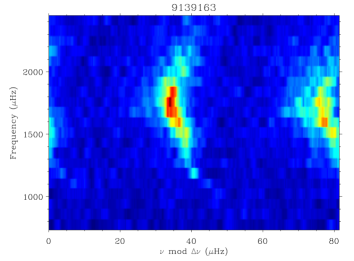
Figure 1: Echelle diagrams of the power spectra of two simple stars (KIC 3427720 and KIC 9139163). The power spectra are normalised by the background and smoothed over 3 $\mu$Hz.

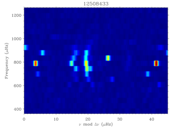
Figure 2: Echelle diagrams of the power spectra of two mixed-mode stars (KIC 5955122 and KIC 12508433). The power spectra are normalised by the background and smoothed over 3 $\mu$Hz. The $l=1$ ridges are broken and pass through the $l=0-2$ ridges; the plot on the left hand side shows an example of a mixed-mode star with the $l=1$ modes not aligned along a ridge but still passing through the $l=0-2$ ridges. The plot on the right hand side shows a faint $l=3$ ridge at 32 $\mu$Hz.

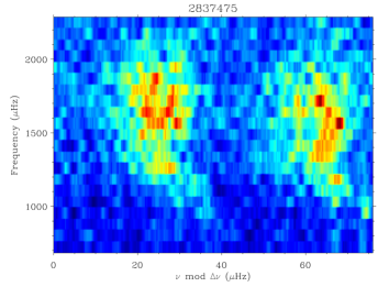
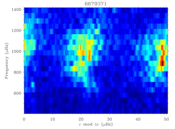
Figure 3: Echelle diagrams of the power spectra of two F-like stars (KIC 2837475 and KIC 6679371). The power spectra are normalised by the background and smoothed over 3 $\mu$Hz.

2 Time series and power spectra

Kepler observations are obtained in two different operating modes: long cadence (LC) and short cadence (SC) (Gilliland et al., 2010; Jenkins et al., 2010). This work is based on SC data. For the brightest stars (down to Kepler magnitude, $Kp\approx 12$), SC observations can be obtained for a limited number of stars (up to 512 at any given time) with a faster sampling cadence of 58.84876 s (Nyquist frequency of $\sim$ 8.5 mHz), which permits a more precise transit timing and the performance of asteroseismology. Kepler observations are divided into three-month-long quarters (Q). A subset of 61 solar-type stars observed during quarters Q5, Q6, and Q7 (March 22, 2010 to December 22, 2010) were chosen because they have oscillation modes with high signal-to-noise ratios. This length of data gives a frequency resolution of about 0.04 $\mu$Hz.

To maximise the signal-to-noise ratio for asteroseismology, the time series were corrected for outliers, occasional jumps, and drifts (see García et al., 2011), and the mean levels between the quarters were normalised. Finally, the resulting light curves were high-pass filtered using a triangular smoothing of width of one day, to minimise the effects of the long-period instrumental drifts. The typical amount of data missing from the time series ranges from 3% to 7%, depending on the star. All the power spectra were produced by one of the co-authors using the Lomb-Scargle periodogram (Scargle, 1982), properly calibrated to comply with Parseval’s theorem (see Appourchaux, 2011).

3 Star categories

To simplify the extraction of mode parameters, three categories of star were identified: simple (sun-like), F-like (also known as the HD49933 syndrome), and mixed modes. The categorisation was performed using the échelle diagram that was first introduced by Grec (1981). The construction of the diagram is based on the low-degree modes being essentially equidistant in frequency for a given $l$, with a typical spacing of the large separation ($\Delta\nu$). The equidistance of the mode frequency $\nu_{nl}$ is the result of an approximation derived by Tassoul (1980) as

$$\nu_{nl}\approx\Delta\nu\left(n+\frac{l}{2}+\epsilon\right)-\delta_{nl},$$ (1)

where $l$ is the degree of the mode, $n$ is the radial order, $\epsilon$ is a parameter related to stellar surface properties, and $\delta_{nl}$ is the small separation. The spectrum is cut into pieces of length $\Delta\nu$, which are stacked on top of each other. Since the modes are not exactly equidistant in frequency, the échelle diagram shows up power due to the modes as curved ridges. Examples of these échelle diagrams are given in Figs. 1 to 3, which represents the three main categories used in this paper. Fig 1 shows examples for simple stars. Fig 2 shows examples for mixed-mode stars where an avoided crossing is present. Fig 3 shows examples for F-like stars, which are hotter stars (spectral type F, having large linewidths).

Figure 4 shows the measured median large-frequency-separation of the 61 stars as a function of their effective temperature, together with their categories resulting from the visual assessment of the échelle diagram. Out of the 61 stars, we have 28 simple stars, 15 F-like stars, and 18 mixed-mode stars. Figure 4 shows that the boundary between simple stars and F-like stars is about 6400 K, which roughly corresponds to a linewidth at maximum mode height of about 4 $\mu$Hz (Appourchaux et al., 2012). For these F-like stars, the frequency separation between the $l=0$ and $l=2$ modes (=small separation) ranges from 4 $\mu$Hz to 12 $\mu$Hz, which, combined with a linewidth of at least 4 $\mu$Hz, explains why the detection of the $l=0$ and 2 ridges is more difficult for these stars.

4 Mode parameter extraction

4.1 Power spectrum model

Table 1: Characteristics of the fit performed by each fitting group. The first column provides the fitter identification; the fitter in italics indicates whether it was a final fitter. The second column provides methods used by the fitters. The third column provides the category of stars fitted; the category in italic indicates which stars were finally fitted. The fourth column provides the number of identifications used. The fifth column provides the number of parameters used per order. The sixth column provides the number of additional parameters common to the modes and the background. The seventh column provides the number of fitted orders. The eighth column provides the range over which the fit is performed. The last column provides how the error bars are computed. The final fitters are indicated in bold. MLE stands for maximum likelihood estimators. MCMC stands for Monte Carlo Markov chain.

Fitter	Method	Star	Iden.	Param.	Add.	Orders	Window	Error
		category		per order	parameters		size
Appourchaux, IAS	MLE Globala	simple / mixed-mode	1	5	5	$\leq$20	$\leq 20\Delta\nu$	Hessian
Howe, NSO	MLE Globalb	simple / mixed-mode	1	5	5	$\leq$15	$\leq 15\Delta\nu$	Hessian
Salabert, A2Z	MLE Globala	simple / mixed-mode	1	5	5	$\leq$15	$\leq 15\Delta\nu$	Hessian
Chaplin, BIR	MLE Pseudo-globalc	simple / mixed-mode	1	5	4	$\leq$20	$\Delta\nu$, $\leq 20\Delta\nu$	Hessian
Deheuvels, YAL	MLE Globala	simple / mixed-mode	1	5	6	$\leq$16	$\leq 16\Delta\nu$	Hessian
Antia, TAT	MLE Locald	simple / mixed-mode	1	12	None	$\leq$15	$\Delta\nu$	Hessian
Verner, QML	MLE Globala	simple / mixed-mode	1	5	5	$\leq$14	$\leq 14\Delta\nu$	Hessian
Benomar, SYD	MCMCe	F-like	2	5	10	$>$10	$>10\Delta\nu$	Credible
Gruberbauer, MAR	Nested samplingf	F-like	2	5	5	$\leq$15	$\leq 15\Delta\nu$	Credible
Handberg, AAU	MCMCg	F-like	2	5	5	$>$10	$>10\Delta\nu$	Credible

• Appourchaux et al. (2008)

• derived from Howe & Hill (1998)

• Fletcher et al. (2009)

• Anderson et al. (1990)

• Benomar et al. (2009a)

• Gruberbauer et al. (2009); Feroz et al. (2009)

• Handberg & Campante (2011)

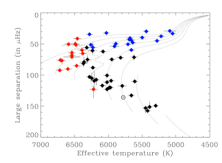
Figure 4: Large separation as a function of effective temperature for the stars in this study; (black) simple stars, (blue) mixed-mode stars, (red) F-like stars, and ($\odot$) the Sun. The effective temperatures were derived from Pinsonneault et al. (2012) except where noted in Table 2. The uncertainties in the large separation represent the minimum and maximum variations with respect to the median measured in this study (see Table 2); some of these uncertainties are within the thicknesses of symbols. The dotted lines are evolutionary tracks for stars of mass from 0.8 M_⊙(farthest right) to 1.5 M_⊙ (farthest left), in steps of 0.1 M_⊙ derived from Christensen-Dalsgaard & Houdek (2010) for solar metallicity.

The mode parameter extraction was performed by ten teams of fitters whose leaders are listed in Table 1. The power spectra were modelled over a frequency range typically covering 10 to 20 large separations (=$\Delta\nu$). The background was modelled using a multi-component Harvey model (Harvey, 1985), each component with two parameters, and a white noise component. The background was fitted prior to the extraction of the mode parameters and then held at a fixed value. For each radial order, the model parameters were mode frequencies (one each for $l$=0,1,2), a single mode height (with assumed ratios of $h_{1}/h_{0}=1.5$, $h_{2}/h_{0}$=0.5 where the subscript refers to the degree), and a single mode linewidth. The ratios taken in this paper are typical of those expected for Kepler stars (Ballot et al., 2011a). In the case of the AAU fitter only, the $l=0$ linewidths were fitted and the linewidths of the other degrees were interpolated in between two $l=0$ mode linewidths. The relative heights $h_{(l,m)}$ (where $m$ is the azimuthal order) of the rotationally split components of the modes depend on the stellar inclination angle, as given by Gizon & Solanki (2003). For each star, the rotational splitting and stellar inclination angle were chosen to be common across all the modes. The mode profile was assumed to be Lorentzian. We used a single Harvey component for all stars other than the 16 stars fitted by QML for which we used a double component. In total, the number of free parameters for 15 orders was at least $5\times 15+2=77$.

The two models described above were used to fit the parameters of 46 stars (28 simple and 18 mixed-mode) using maximum likelihood estimators (MLE). Formal uncertainties in each parameter were derived from the inverse of the Hessian matrix (for more details on MLE, significance, and formal errors, see Appourchaux, 2011).

The 15 F-like stars were fitted with a Bayesian approach using different sampling methods. Both SYD and AAU employed Monte Carlo Markov chain (MCMC) (Benomar et al., 2009a; Handberg & Campante, 2011), while MAR used nested sampling via the code MultiNest (Feroz et al., 2009). For the latter sampling approach, the large number of parameters forced us to use MultiNest’s constant-efficiency, mono-modal mode. The priors on the central frequency and inclination angle were uniform. The prior on the splitting was either uniform in the range $0-15\leavevmode\nobreak\ \mu$Hz (MAR) or a combination of a uniform prior in the range $0-2\leavevmode\nobreak\ \mu$Hz and a decaying Gaussian (SYD, AAU). The priors on mode height were modified Jeffreys priors (Jeffreys, 1939; Benomar et al., 2009a; Gruberbauer et al., 2009), and the priors on the linewidth were either uniform (MAR) or modified Jeffreys priors (SYD, AAU). The error bars were derived from the marginal posterior distribution of each parameter. Each Bayesian fitter had seven stars to fit: four stars + three common stars. The latter were used for comparison with the Bayesian methods. Priors on the frequencies were set after visual inspection of the power spectrum. Modes of degree $l=2$ were assumed to be on the low-frequency side of the $l=0$ (i.e., the small spacing $d_{02}$ was assumed to be positive). To avoid spurious results, two of the Bayesian fitters (SYD, MAR) also used a smoothness condition on the frequency for each degree, in a similar way to Benomar et al. (2012b).

Table 1 provides a summary of how the different fits were performed.

4.2 Initial guesses for parameters

Of all the parameters describing the modes, the frequencies are the most difficult to guess. Given the number of stars, initial guesses for these mode frequencies were obtained using different techniques:

• The automatic detection of modes based on the values of $\Delta\nu$ and $\nu_{\rm max}$ (see Verner et al., 2011, and references therein), that were then manually tweaked if required.

• Visual detection using the échelle diagram (especially for mixed-mode stars).

• Derivation from fitted parameters obtained from previous reported observations of the stars (see Table 2).

The degree tagging could then be done quite easily for the simple and mixed-mode stars (see Figs. 1 and 2). The mere visual assessment of the échelle diagrams was enough to permit the tagging of the ridges with the proper degree where the $l=1$ stands alone, while the $l=0-2$ pair appears as a double ridge. For the mixed-mode stars, the tagging was also done by inspection of the échelle diagram, but required the input of model frequencies as the $l=1$ modes go through the $l=0-2$ ridges; some ambiguity could be caused by the avoided crossing. For the F stars, the fit was performed for both possible identifications ($l=0-2$ and $l=1$, or vice versa), and the model probabilities were calculated to obtain the most likely identification (Benomar et al., 2009a; Handberg & Campante, 2011). For these latter stars, other tools are available that compare the measured value of $\epsilon$ (see Eq. 1) with that of the theoretical values derived for other stars with similar effective temperatures (White et al., 2011).

4.3 Fitting procedure

The steps that we adopted to perform the fit are as follows:

1. We fit the power spectrum as the sum of a background made of a combination of Lorentzian profiles (one or two) and white noise, as well as a Gaussian oscillation mode envelope with three parameters (the frequency of the maximum mode power, the maximum power, and the linewidth of the mode power).

2. We fit the power spectrum with $n$ orders using the mode profile model described above, with no splitting and the background fixed as determined in step 1

3. We follow step 2 but define the splitting and the stellar inclination angle as free parameters, and then apply a likelihood ratio test to assess the significance of the fitted splitting and angle.

The steps above were sometimes varied slightly depending on the assumptions that were made. For instance, the mode height ratio could instead be defined as a free parameters to study the impact of its variations on the derivation of the mode parameters such as linewidth and mode height.

5 Derivation of mode frequency set

The derivation of a single frequency set from the several sets obtained by different fitters has been a source of considerable concern since we started this work. The measurements performed by Kepler for a given star are done only by this mission; there is no additional source of photometry. Hence, this single measurement of oscillation modes in the photometry of a given star must provide a single frequency set. The main question that arose was how to derive a single frequency set from the different fits.

We now explain the chain of thought that led to the procedure used in this paper. This procedure had constantly evolved until we reached the final procedure. Since anyone having to derive a common data set from several data sets derived from a single observable will face the same challenge as we faced, it is useful to understand how we decided on this procedure to avoid repeating the same chain of thoughts.

The final procedure can be applied to any data set to be derived from a single observable, such as mode linewidth, mode amplitude, and so forth. An example of the application of this procedure for mode linewidth can be found in Appourchaux et al. (2012).

Hereafter, we describe the final procedure in three steps. The first step is common to all variants of the procedure, while the second step had several versions. We present all the second-step versions used, including the step used in the final procedure.

5.1 Common first step

The goal of the first step is to provide an average frequency set and to quantify how a given frequency set provided by a fitter differs from the average.

5.1.1 Rejection of outliers

For a given ($n,l$) mode, one frequency is derived from several (if not all) fitters and outliers may need to be rejected. The rejection of outliers can be done either using the well-known 3-$\sigma$ threshold or using Peirce’s criterion (Peirce, 1852). The main disadvantage of the 3-$\sigma$ threshold is that it is not applicable when the number of measurements is small. Peirce’s criterion explicitly assumes that the number of measurements is small and that the root mean square (rms) deviation can be corrected for the rejection of outliers. Peirce’s criterion is based on rigourous probability calculation and not on any ad hoc assumption. To cite Peirce’s explanation of his criterion: “The proposed observations should be rejected when the probability of the system of errors obtained by retaining them is less than that of the system of errors obtained by their rejection multiplied by the probability of making so many, and no more, abnormal observations.” This logic calls for an iterative assessment of the rejection when one or more datasets are rejected. The iteration stops when no improvement is possible.

Following the work of Gould (1855), we implemented Peirce’s criterion for a sample of $x_{i}$ as follows:

1. We compute the mean value $x_{m}$ and rms deviation $\sigma$ of a data set $x_{i}$.

2. We compute the rejection factor $r$ by solving Eq. (D) of Gould (1855), assuming one doubtful observation.

3. We reject data if $|x_{i}-x_{m}|>r\sigma$.

4. If $n$ data have been rejected then we compute the new rejection factor $r$, assuming $n+1$ doubtful observations.

5. We repeat steps 3 to 4 until no more data are rejected.

The assumption behind Peirce’s criterion is that all the observed data have the same statistical distribution, i.e., the same mean and standard deviation. In our case, this assumption is valid because all the methods used (see Table 1) are either exactly or approximately akin to MLE, so that the error bars in our mode frequencies are locally related to the curvature of the MLE at the location of the maximum.

The rejection of outliers following Peirce’s criterion was implemented as an option for the common first step.

5.1.2 Deviation from the average frequency set

For a given star and for a given ($n,l$) mode, one computes the mean mode frequency $\langle\nu_{n,l}\rangle$ from the frequencies provided by the fitters who detected this mode. The frequency set consisting of the data $\langle\nu_{n,l}\rangle$ is then designated as the average frequency set. For each fitter labelled k, one then computes for each mode the mean normalised rms deviation from the mean mode frequency $\langle\nu_{n,l}\rangle$, and the average deviation over all modes:

$$\delta_{{\rm k}}=\sqrt{\frac{1}{N_{\rm k}}\sum_{n,l}\frac{\left(\nu_{n,l}^{\rm k}-\langle\nu_{n,l}\rangle\right)^{2}}{(\sigma_{n,l}^{\rm k})^{2}}},$$ (2)

where, $\nu_{n,l}^{\rm k}$ and $\sigma_{n,l}^{\rm k}$ are the frequency and its uncertainty returned by fitter k, and $N_{\rm k}$ is the number of modes fitted by the fitter k. The normalised rms deviation $\delta_{{\rm k}}$ then provides a way of assessing how far the fitter k deviates from the average value of the frequencies.

5.2 Second step

The goal of the second step is to provide the selected frequency set using the results of the first step. The selected frequency set is then used for either subsequent modelling or fitting.

5.2.1 Method 1

Peirce’s criterion is not applied. The selected mode set comprises the modes for which the frequencies of all fitters agree, within their own $1-\sigma$ error bars, with the average frequency set. This set is supplemented by additional modes for which the frequencies of only a smaller group of the fitters agree, within their own $1-\sigma$ error bars, with the average frequency set. The selected frequency set of the fitter with the smallest $\delta_{{\rm k}}$ is then designated the reference fit. This method was used by Appourchaux et al. (2008) for HD49933.

The major drawback of this method is that if a single fitter disagrees, owing to the very small error bars of their measurements, then there is no selected set. In addition, the good modes fitted by a single fitter are automatically rejected.

5.2.2 Method 2

Peirce’s criterion is not applied. Instead of having only one mode set, we derive minimal and maximal mode sets as follows. The minimal mode set is, as previously, the one for which all fitters agree within their own $1-\sigma$ error bars, with the average frequency set. The maximal mode set is made up of the frequencies for which at least two fitters agree within their own $1-\sigma$ error bars, with the average frequency set. The frequency set of the fitter with the smallest $\delta_{{\rm k}}$ for the minimal mode set is then designated the minimal frequency set, and the frequency set of the fitter with the smallest $\delta_{{\rm k}}$ for the maximal mode set is designated the maximal frequency set. This method was used by Metcalfe et al. (2010) for the Kepler star KIC 11026764.

There are several drawbacks to this method. Firstly, the minimal and maximal frequency sets can be produced by different fitters. This “feature” is a great nuisance when one derives different stellar models for the same star, that are the result of two different frequency sets. In addition, the drawbacks of method 1 are not alleviated at all by this scheme, and the minimal set may not exist at all.

5.2.3 Method 3

This is the same as method 2 but with the Peirce’s criterion applied. The drawbacks are the same as method 2.

5.2.4 Method 4

Peirce’s criterion is applied. We still derive a minimal and a maximal mode set, but now, for deriving the minimal mode set, we use a voting scheme. The minimal mode set contains the modes for which at least half the fitters agree within their own $1-\sigma$ error bars, with the average frequency set. The maximal mode set contains the modes for which at least two fitters agree within their own $1-\sigma$ error bars, with the average frequency set. The frequency set of the best fitter with the smallest $\delta_{{\rm k}}$ for the minimal mode set is then designated as the best frequency set. The maximal and minimal frequency sets are then derived from the minimal and maximal mode sets of the best fitter. With such a scheme, one of the drawbacks of method 2 is removed: the two sets come from the same best fitter. This fourth method was used by Mathur et al. (2011), Campante et al. (2011), and Howell et al. (2012). The remaining drawback is that the good modes fitted by only one fitter are still rejected.

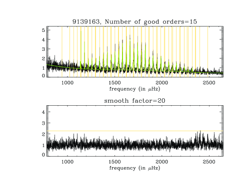
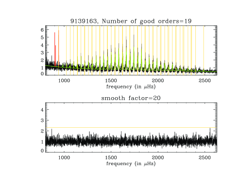
Figure 5: Detection of left-out modes. All power spectra are shown as a function of frequency smoothed over 20 bins. Before the refit: (Top, left) Power spectrum of KIC 9139163 with the fitted model with accepted modes (green) and with the guess frequencies provided by the fitters (orange lines). (Bottom, left) Power spectrum normalised to the fitted model; the orange horizontal line indicates the level at which the null hypothesis is rejected at the 1% level. After the refit: (Top, right) Power spectrum of KIC 9139163 with the fitted model for either accepted modes (green), rejected modes (red), or the guess frequencies provided a posteriori by the fitters (orange lines). (Bottom, right) Power spectrum normalised to the fitted model; the orange horizontal line indicates the level at which the null hypothesis is rejected at the 1% level.

5.3 Third step: the final fitter

The goal of the third step is to provide a single homogenous frequency set using the maximal frequency set as guess frequencies. This third step was used by Metcalfe et al. (2012) for 16 Cyg A/B stars, by Mathur et al. (2012) for 22 Kepler stars, and in this paper.

The current solution that we adopt here is to ensure that a final fitter refits the spectrum using the maximal mode set derived in method 4 of the Second Step, and also using some visual assessment and/or statistical tests where all the modes are included. In this case, even the modes provided by only one fitter are included. In addition, the solution of having a final fitter provide the frequency sets produces a homogenous data sets with systematic errors traceable to a single origin. This is now the current strategy used to provide seismic parameters of the solar-like stars from the Kepler data.

After having applied the procedure described above, the 61 stars were fitted by 4 final fitters: BIR fitted 14 mixed-mode stars, IAS fitted 16 simple stars, QML fitted 13 simple and 3 mixed-mode stars, and MAR fitted the 15 F-like stars (see Table 1). The division of the work for the MLE-based fit was based upon the availability of both computer and personal time. As for the F-like stars, the work was performed by a single fitter for consistency.

6 Product and quality assurance of the frequencies

After producing the frequency sets for each star, we needed to assess whether the frequencies provided were of significant quality to be used in subsequent stellar modelling. Several tests are at our disposal for gauging the likelihood of having either a good or bad mode. Here the term bad refers to a mode that is obviously either a noise peak mistaken for a mode (for example, at low frequency where the mode linewidth is narrow) or to a broad spurious excess of power at high frequency (where the mode linewidth is large). Statistical tests fall into two major categories: frequentist and Bayesian. Both type of tests are addressed in Appourchaux (2011).

6.1 Significance of fitted parameters

To assess the significance of a given mode, one can use the likelihood ratio (LR) test, which is a frequentist test. The test simply checks the likelihood that the fitted mode is due to spurious noise, i.e., it tests whether the null or H₀ hypothesis can be accepted or rejected. The test consists of computing $\log(\Lambda)$, where $\Lambda$ is the ratio of the likelihood obtained when fitting $m$ parameters to the likelihood obtained when fitting $n$ parameters ($m>n$). The test statistic $-2\log(\Lambda)$ is then known to be distributed as $\chi^{2}$ with ($m-n$) degrees of freedom (d.o.f) under the null hypothesis.

6.1.1 Splitting and inclination angle

The LR test can be simply applied to check the significance of the splitting and inclination angle, which are usually assumed to be common amongst the fitted orders. The LR test is applied as follows:

1. We fit the whole spectrum with all the parameters apart from the angle and splitting (both set to 0). We compute the likelihood of the fit.

2. We fit the whole spectrum with all the parameters, including the angle and splitting, and then compute the likelihood of the fit.

3. We compute LR($p$) ($p=2$).

4. We reject the pair (splitting,angle) at the 1% level.

This test was used to derive the frequencies provided in this paper. However, rotational splitting in these stars is the subject of another study, currently in progress.

6.1.2 Orders and modes

The major drawback of the LR test is that it requires a new fit each time we need to test the significance of several parameters. In our case, since we fitted up to 80 parameters, it became impractical to “switch of” each of the orders in turn, let alone each of the modes. We devised a simplified LR test based on the assumption that some of the parameters are independent of each other. For example, if we remove a given order then to a good approximation this will not affect the result of the other orders. Therefore, we applied the simplified LR test as follows:

1. We fit the whole spectrum with all the parameters and compute likelihood of the fit.

2. We “switch of” orders (one at a time) and compute the new likelihood without making a new fit.

3. We compute LR($n$) ($n=5$, three mode frequency, one linewidth, one amplitude).

4. We reject order at the 1% level.

If the whole order is rejected, then we apply the same simplified LR test to each mode within it, with the same cut level ($n=1$, 1 frequency).

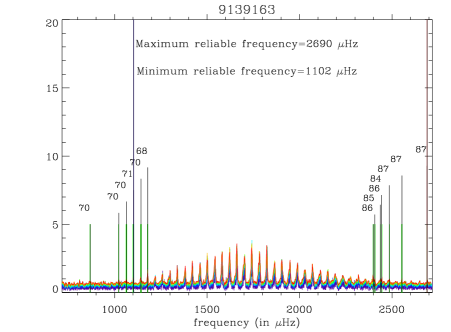
Figure 6: Smoothed power spectrum normalised to the detection $x_{\rm det}$ as a function of frequency for several smoothing factors (several colours; the redder the colour the higher the smoothing factor, which varies from 2 to 70 frequency bins). The short vertical black lines show the minimum and maximum frequency detected with a single smoothing factor and their associated posterior probabilities ($p(x_{\rm det}|{\rm H}_{1})$) for H₁, in %. When the frequency is detected several times to within 4 $\mu$Hz, only the highest posterior is shown. The long vertical black lines show the minimum minimorum and maximum maximorum frequencies.

6.2 Are all modes detected?

When the power spectra were fitted, the frequencies of the modes were guessed using either a simplified detection test that looks for high peaks around the region of maximum mode power, or a search for clumps of power in several adjacent or close bins. We were also able to guess the mode frequencies by eye in the échelle diagram. These statistical tests or visual tests rely either on testing the null hypothesis (frequentist) or explicit knowledge of the mode frequency behaviour (Bayesian). Hereafter, we detail both types of tests that were used to ensure that all modes are detected.

6.2.1 Frequentist test

After performing the fit, we computed the ratio of the power spectrum to the fitted model. Since the modes are stochastically excited harmonic oscillators, the resulting ratio was simply the power spectrum of the forcing functions (mode excitation + noise), which is distributed as a $\chi^{2}$ distribution with two d.o.f. The resulting ratio power spectrum could then be smoothed to detect signals that are spread over several bins. The left-hand side of Fig. 5 shows the result of applying this procedure: power is clearly detected above 2300 $\mu$Hz. The right-hand side of Figure 5 shows the result of applying the procedure after including the missing modes: nothing is detected in the smoothed ratio power spectrum above a frequency of 2300 $\mu$Hz. In Fig. 5, we note that the modes at low frequencies below 1100 $\mu$Hz are not detected by the mere application of a single smoothing factor. We devised a more sensitive test that allows the detection of these modes at low frequency, but also the detection of modes at higher frequencies that are not provided by the fitters.

6.2.2 Bayesian approach

The previous test described in Sect. 6.2.1 is quite effective in rejecting the null hypothesis but fails to achieve what is required: to provide a quantitative likelihood that a mode has been detected. To achieve this aim, we must instead use some a priori knowledge of the behaviour of the modes at low and high frequencies. Here we used the work of Appourchaux (2004) to detect short-lived modes. This work had been applied to two CoRoT stars (Appourchaux et al., 2009; Deheuvels et al., 2010). We used a variant of the procedure that included a test based on a priori empirical knowledge of the mode linewidth at low and high frequency. The procedure adopted is as follows:

1. We fit the power spectrum as the sum of a background made of a combination of one or two Lorentzian profiles centred at the zero frequency and white noise, with a Gaussian oscillation mode envelope. The combination of the Lorentzian profiles and the white noise provides a model for the observed stellar background noise.

2. We compute the ratio of the power spectrum to the background but put the mode envelope to zero. The signal-to-noise ratio of the modes of oscillation is then the observed power spectrum divided by the modelled background noise. This ratio of the power spectrum to the background contains the modes of oscillation multiplied by the $\chi^{2}$ 2 d.o.f. forcing functions.

3. We smooth the ratio power spectrum over $n$ bins to maximise the signal in power due to modes of oscillation that are distributed over many bins. To maintain the scaling of the signal-to-noise ratio, the smoothed power spectrum must be multiplied by $n$. The smoothing, of course, modifies the statistical distribution, and the modified distribution is known to be $\chi^{2}$ with 2$n$ d.o.f.

4. We accept or reject the H₀ hypothesis with a detection probability of $p_{\rm det}^{\rm win}$ over a window covering half the large separation (=$\Delta\nu_{0}/2$), taking into account that in each window the number of independent bins is $N_{\rm ind}=\Delta\nu_{0}/(2n{\delta\nu})$ where $\delta\nu$ is the frequency resolution of the original power spectrum. The detection probability per independent bin is then $p_{\rm det}=p_{\rm det}^{\rm win}/N_{\rm ind}$. The detection probability we used is $p_{\rm det}^{\rm win}=0.1$ or 10%.

5. To determine the detection level $x_{\rm det}$, we compute the probability $p_{\rm det}$ of observing $x_{\rm det}$ or greater, which is $p_{\rm det}\leavevmode\nobreak\ =\leavevmode\nobreak\ \frac{1}{\Gamma(n)}\int_{x_{\rm det}}^{+\infty}u^{n-1}{\rm e}^{-u}{\rm d}u$ (where $\Gamma$ is the gamma function, and $u$ is a dummy symbol), and then solve this equation for $x_{\rm det}$ given $p_{\rm det}$.

6. In each window, we then select the bins in the smoothed ratio power spectrum that are greater than $x_{\rm det}$, i.e., we reject the H₀ hypothesis.

This procedure from step 1 to step 6 is very similar to the one described in the previous section for the detection of left-out modes.

Additional assumptions are now taken into account in the Bayesian approach. If the H₀ hypothesis is rejected, we can write the detection likelihood, which is given by Eq. (15) of Appourchaux et al. (2009),

$$p(x_{\rm det}|{\rm H}_{0})=\frac{x_{\rm det}^{n-1}{\rm e}^{-x_{\rm det}}}{\Gamma(n)}.$$ (3)

The next step is to derive $p(x_{\rm det}|{\rm H}_{1})$ subject to the H₁ hypothesis, which is to assume that a true mode has been detected. With the many stars at our disposal, we preferred to have an educated a priori knowledge of the mode height and mode linewidth, in lieu of their theoretical model parameters. We can rewrite Eq. (18) (Appourchaux et al., 2009) assuming uniform priors for the mode height and linewidth

$$p(x_{\rm det}|{\rm H}_{1})=\frac{1}{h_{\rm u}W_{\rm u}}\int_{0}^{h_{\rm u}}\int_{0}^{W_{\rm u}}\frac{\lambda^{\nu}}{\Gamma(\nu)}x_{\rm det}^{\nu-1}{\rm e}^{-\lambda{x_{\rm det}}}{\rm d}h^{\prime}{\rm d}W^{\prime},$$ (4)

where $\lambda$ and $\nu$ are the parameters defining the Gamma statistical distribution, $\lambda$ and $\nu$ are functions of $h^{\prime}$ and $W^{\prime}$ with $h^{\prime}$ being the mode height in noise units, $W^{\prime}$ is the mode linewidth (see Appendix A), $h_{\rm u}$ is the maximum mode height, $W_{\rm u}$ is the maximum mode linewidth. This formula is obviously more observer-oriented. Since we wished to detect faint modes at either end of the spectrum, we assumed that the maximum mode height would be no larger than twice the noise, and that the mode linewidth no larger than 1 $\mu$Hz, at low frequency and 10 $\mu$Hz at high frequency. We then computed the posterior probability of H₁ as

$$p({\rm H}_{1}|x_{\rm det})=\left(1+\frac{p(x_{\rm det}|{\rm H}_{0})}{p(x_{\rm det}|{\rm H}_{1})}\right)^{-1}.$$ (5)

The procedure then continues with the steps:

1. From all the frequencies for which the null hypothesis was rejected, we keep the highest and lowest detected frequencies

2. We then compute the posterior probability of H₁ as given by Eq. (5) for these two extreme frequencies.

The steps 1 to 8 are repeated for a range of smoothing factors $n$ from 2 to 70, corresponding to the resolution of 0.08 $\mu$Hz to 2.8 $\mu$Hz. The variable amount of smoothing allows for the detection probability depending on both the smoothing factor and the mode linewidth. The maximum detection probability is reached for different values of the smoothing factor, depending on the mode linewidth.

We then defined the maximum maximorum detectable frequency as the highest detected frequency for which the posterior probability is either greater than 90% or has the highest value if this is lower than 90%. The minimum minimorum frequency was defined as the lowest detected frequency for which the posterior probability is either greater than 90% or has the highest value if this is lower than 90%. Figure 6 provides an example of the application of the procedure.

Table 3 shows an example of an application of the quality assurance test to the fitted frequencies, which can be compared with Figure 5. Figure 7 shows more examples of the application of the procedure resulting in different cases of no detection, no fit, and detection with a posterior probability less than 90%. For the star KIC 7106245, several modes were not detected, as listed in Table 4. For the star KIC 7976303, several modes were not fitted, as listed in Table 5. For the stars KIC 9139151 and KIC 10162436, a few modes were either not detected or not fitted or detected with a posterior probability lower than 90%, as listed in Table 6 and 7, respectively.

The procedure was applied to all stars in this paper irrespective of the final fitter for providing a quality assessment at all the frequencies. If one of the frequencies from the test was not provided by the fitter, we verified whether it could be a mode close to an integer value of the large separation, and then made the most likely degree identification.

The application of the product assurance resulted in 61 tables of frequencies. The mode frequencies of 61 stars are provided in Tables 3 to 7 with the paper, and Tables A.1 to A.56 as online material. All modellers are advised to use all of the mode frequencies labelled OK and to use with caution all other frequencies. In addition, the 61 échelle diagrams are shown in Figs A.1 to A.10, and also as online material.

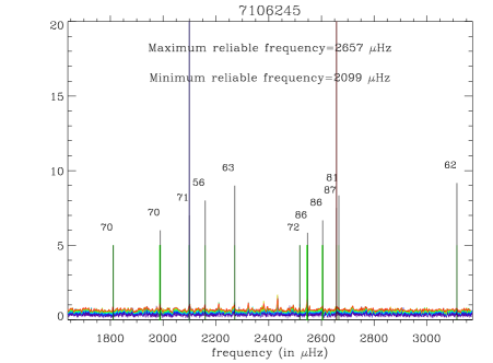
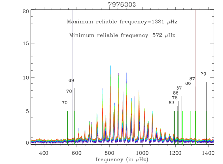
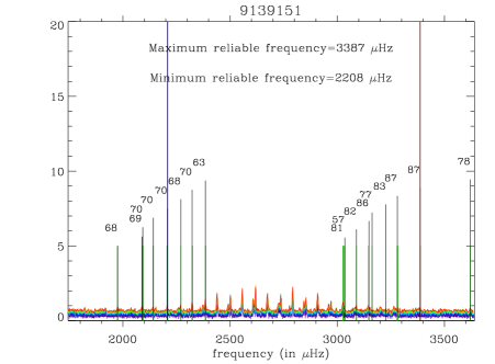
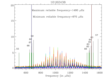
Figure 7: Smoothed power spectrum normalised to the detection $x_{\rm det}$ as a function of frequency for several smoothing factor values (several colours; the redder and the higher the smoothing factor) for four stars (KIC 7106245, KIC 7976303, KIC 9139151, KIC 10162436). The short vertical black lines show the minimum and maximum frequency detected with a single smoothing factor with their associated posterior probability ($p(x_{\rm det}|{\rm H}_{1})$) for H₁, in %. When the frequency is detected several times within 4 $\mu$Hz, only the highest posterior is shown. The long vertical black lines show the minimum minimorum and maximum maximorum frequencies.

7 Conclusions

We have analysed the oscillation power spectra of 61 main sequence and subgiant stars for which we fitted the p-mode parameters. We have divided the stars into three categories related to the visual appearance of their échelle diagrams called simple, F-like, and mixed-mode stars. We have shown that we are now able to perform nearly automated fits of many stellar power spectra derived from Kepler light curves. There are two steps that still require manual intervention: the identification of the star category provided by the échelle diagram and the derivation of first-guess frequencies. In the future, we plan to reduce the amount of manual intervention by using the areas delimited in the ($\Delta\nu$, $T_{\rm eff}$) diagram of Fig. 4 to identify the star category; and by using the asymptotic relation of frequencies used by Benomar et al. (2012a) to derive automated guess frequencies.

We devised a procedure to use the mode frequencies from several fitters to choose a single fitter to re-fit all the spectra (within workload constraints). When the power spectra are fitted, we are now also able to make an automated assessment of the fit quality and the mode frequencies obtained; we give several techniques for this assessment. We provide the échelle diagrams of 61 stars and the associated list of mode frequencies for these stars.

Table 2: Table of key stellar parameters. The first three columns provide the KIC, HIP, and HD numbers. The fourth column provides the effective temperature and its error bar taken from Pinsonneault et al. (2012). The fifth column provides the Kepler magnitude. The sixth column gives the median of the large separation as measured using the mode frequencies given in this paper. The seventh column provides the frequency of the maximum of oscillation power. The eighth column gives the number of detected modes. The penultimate column gives the star category. The last column provides notes on whether the star has been previously observed or has mixed modes.

KIC	HIP	HD	$T_{\rm eff}$ (K)	Kp	$\Delta\nu$ ($\mu$Hz)	$\nu_{\rm max}$($\mu$Hz)	Number of modes	Star category	Notes
1435467	-	-	6541 $\pm$ 126	8.9	70.9	1324	45	F-like
2837475	-	-	6710 $\pm$ 61	8.5	76.0	1522	45	F-like
3424541	-	-	6460 $\pm$ 55	9.7	41.3	712	37	F-like
3427720	-	-	5970 $\pm$ 52	9.1	120.1	2574	30	simple
3632418	94112	179070	6235 $\pm$ 70	8.2	60.7	1084	34	simple	c, d
3733735	94071	178971	6720 $\pm$ 56	8.4	92.4	2041	43	F-like
3735871	-	-	6220 $\pm$ 61	9.7	123.1	2633	25	F-like
5607242	-	-	5680 $\pm$ 51	10.7	40.6	610	39	mixed modes	$\dagger$
5955122	-	-	5890 $\pm$ 51	9.3	49.6	826	38	mixed modes	$\dagger$
6116048	-	-	6020 $\pm$ 51	8.4	100.7	2020	34	simple	c
6508366	-	-	6480 $\pm$ 56	9.0	51.6	959	45	F-like
6603624	-	-	5610 $\pm$ 51	9.1	110.3	2339	31	simple	b, c
6679371	-	-	6590 $\pm$ 56	8.7	50.4	908	44	F-like
6933899	-	-	5820 $\pm$ 50	9.6	72.1	1362	33	simple	c
7103006	-	-	6390 $\pm$ 56	8.9	59.9	1072	46	F-like
7106245	-	-	6020 $\pm$ 51	10.8	111.6	2323	16	simple
7206837	-	-	6360 $\pm$ 56	9.8	79.0	1556	40	simple
7341231	-	-	5091 $\pm$ 91	9.9	29.0	404	44	mixed modes	e, $\dagger$
7747078	91918	-	5910 $\pm$ 70	9.5	53.7	977	37	mixed modes	d, $\dagger$
7799349	-	-	5050 $\pm$ 45	9.5	33.2	560	40	mixed modes	$\dagger$
7871531	-	-	5390 $\pm$ 47	9.3	151.3	3344	25	simple
7976303	-	-	6260 $\pm$ 51	9.0	51.3	826	36	mixed modes	$\dagger$
8006161	91949	-	5300 $\pm$ 46	7.4	149.4	3444	26	simple	c
8026226	-	-	6280 $\pm$ 52	8.4	34.4	520	40	mixed modes	$\dagger$
8228742	95098	-	6080 $\pm$ 51	9.4	62.1	1153	33	simple	c
8379927	97321	187160	5990 $\pm$ 52	7.0	120.4	2669	37	simple
8394589	-	-	6210 $\pm$ 52	9.5	109.4	2336	32	simple
8524425	-	-	5660 $\pm$ 51	9.7	59.7	1078	33	mixed modes	$\dagger$
8694723	-	-	6310 $\pm$ 56	8.9	75.1	1384	49	simple
8702606	-	-	5500 $\pm$ 51	9.3	39.7	626	40	mixed modes	$\dagger$
8760414	-	-	5795 $\pm$ 70	9.6	117.4	2349	31	simple	c, d
9025370	-	-	5660 $\pm$ 52	8.8	132.8	2864	23	simple
9098294	-	-	5960 $\pm$ 51	9.8	109.1	2241	27	simple
9139151	92961	-	6090 $\pm$ 52	9.2	117.0	2610	34	simple
9139163	92962	-	6370 $\pm$ 56	8.3	81.4	1649	55	simple
9206432	93607	-	6470 $\pm$ 56	9.1	85.1	1822	51	F-like
9410862	-	-	6180 $\pm$ 51	10.7	107.5	2034	24	simple
9574283	-	-	5440 $\pm$ 47	10.7	29.7	448	32	mixed modes	$\dagger$
9812850	-	-	6380 $\pm$ 55	9.5	65.3	1186	41	F-like
9955598	-	-	5450 $\pm$ 47	9.4	153.1	3379	26	simple
10018963	-	-	6230 $\pm$ 52	8.7	55.5	988	41	simple	c
10162436	97992	-	6320 $\pm$ 53	8.6	55.9	1004	45	simple
10355856	-	-	6540 $\pm$ 56	9.2	68.3	1210	40	F-like
10454113	92983	-	6246 $\pm$ 58	8.6	105.2	2313	43	simple
10644253	-	-	6020 $\pm$ 51	9.2	123.0	2866	27	simple
10909629	-	-	6490 $\pm$ 61	10.9	49.7	813	35	F-like
10963065	-	-	6280 $\pm$ 51	8.8	102.9	2071	34	simple	c
11026764	-	-	5710 $\pm$ 51	9.3	50.4	885	30	mixed modes	a, b, $\dagger$
11081729	-	-	6600 $\pm$ 62	9.0	90.2	1820	45	F-like
11193681	-	-	5690 $\pm$ 51	10.7	42.9	752	32	mixed modes	$\dagger$
11244118	-	-	5620 $\pm$ 51	9.7	71.4	1352	31	simple	c
11253226	97071	186700	6690 $\pm$ 56	8.4	76.9	1637	30	F-like
11395018	-	-	5640 $\pm$ 51	10.8	47.7	840	26	mixed modes	$\dagger$
11414712	-	-	5660 $\pm$ 51	8.5	44.1	730	44	mixed modes	$\dagger$
11717120	-	-	5220 $\pm$ 48	9.3	37.6	555	42	mixed modes	$\dagger$
11771760	-	-	6030 $\pm$ 51	11.4	32.2	505	37	mixed modes	$\dagger$
11772920	-	-	5420 $\pm$ 51	9.7	157.6	3439	23	simple
12009504	-	-	6230 $\pm$ 51	9.3	88.1	1768	34	simple	c
12258514	95568	183298	5950 $\pm$ 51	8.1	74.8	1449	34	simple	c
12317678	97316	-	6540 $\pm$ 55	8.7	64.1	1162	51	F-like
12508433	-	-	5280 $\pm$ 47	9.5	45.0	758	36	mixed modes	$\dagger$

• Already analysed by Metcalfe et al. (2010), Chaplin et al. (2011), Mathur et al. (2012), respectively.

• Effective temperature from Bruntt et al. (2012) and Casagrande et al. (2010), respectively

• Star with mixed modes for which $\Delta\nu$ was derived from the $l=0$ modes only

Table 3: Frequencies for KIC 9139163. The first column is the degree. The second column is the frequency. The third column is the 1-$\sigma$ uncertainty quoted when the mode is fitted. The last column provides an indication of the quality of the detection: OK indicates that the mode was correctly detected and fitted; Not detected indicates that the mode was fitted but not detected by the quality assurance test and Not fitted indicates that the mode was detected with a posterior probability provided by the quality assurance test. When an uncertainty and a posterior probability are quoted, it means that the mode is fitted but detected using the quality assurance test with a probability lower than 90%.

Degree	Frequency ($\mu$Hz)	1-$\sigma$ error ($\mu$Hz)	Comment
0	986.105	1.130	Not detected
0	1064.982	0.690	0.703
0	1142.941	0.230	OK
0	1221.476	0.544	OK
0	1301.395	0.332	OK
0	1383.093	0.366	OK
0	1464.189	0.381	OK
0	1544.456	0.317	OK
0	1623.952	0.380	OK
0	1703.1000	0.340	OK
0	1785.675	0.330	OK
0	1866.729	0.420	OK
0	1949.424	0.391	OK
0	2031.407	0.706	OK
0	2114.451	0.607	OK
0	2195.335	1.219	OK
0	2276.836	0.928	OK
0	2359.243	1.229	OK
0	2444.022	1.734	OK
0	2689.590	Not fitted	0.873
1	1023.888	0.576	0.705
1	1102.258	0.427	OK
1	1179.797	0.181	OK
1	1258.873	0.451	OK
1	1340.250	0.280	OK
1	1421.435	0.305	OK
1	1502.036	0.292	OK
1	1581.801	0.270	OK
1	1661.689	0.269	OK
1	1742.582	0.261	OK
1	1824.248	0.271	OK
1	1905.932	0.376	OK
1	1989.005	0.401	OK
1	2071.453	0.469	OK
1	2153.260	0.526	OK
1	2235.598	0.876	OK
1	2319.330	0.806	OK
1	2399.494	0.844	OK
1	2485.579	1.291	OK
1	2553.800	Not fitted	0.866
2	982.173	1.756	Not detected
2	1057.448	0.955	Not detected
2	1135.556	3.432	OK
2	1216.915	1.141	OK
2	1294.411	0.609	OK
2	1377.256	0.924	OK
2	1458.740	0.863	OK
2	1538.360	0.805	OK
2	1620.012	1.032	OK
2	1696.864	0.684	OK
2	1779.203	0.601	OK
2	1860.596	1.060	OK
2	1942.470	0.960	OK
2	2025.300	1.424	OK
2	2105.809	1.195	OK
2	2189.691	2.425	OK
2	2265.891	1.291	OK
2	2352.782	3.939	OK
2	2437.430	2.378	OK

Table 4: Frequencies for KIC 7106245. The first column is the degree. The second column is the frequency. The third column is the 1-$\sigma$ uncertainty quoted when the mode is fitted. The last column provides an indication of the quality of the detection: OK indicates that the mode was correctly detected and fitted; Not detected indicates that the mode was fitted but not detected by the quality assurance test and Not fitted indicates that the mode was detected with a posterior probability provided by the quality assurance test. When an uncertainty and a posterior probability are quoted, it means that the mode is fitted but detected using the quality assurance test with a probability lower than 90%.

Degree	Frequency ($\mu$Hz)	1-$\sigma$ error ($\mu$Hz)	Comment
0	1718.954	0.529	Not detected
0	1939.538	0.042	Not detected
0	2049.668	0.383	Not detected
0	2159.780	0.251	OK
0	2271.402	0.207	OK
0	2382.167	0.235	OK
0	2494.757	0.336	OK
0	2605.011	0.688	OK
1	1770.100	0.248	Not detected
1	1989.784	0.038	0.703
1	2100.640	0.426	OK
1	2211.749	0.270	OK
1	2323.982	0.281	OK
1	2434.871	0.192	OK
1	2546.874	0.278	OK
1	2659.004	0.864	OK
2	1707.675	0.600	Not detected
2	1931.915	0.041	Not detected
2	2043.194	0.678	Not detected
2	2152.546	0.441	OK
2	2264.302	0.380	OK
2	2375.609	0.398	OK
2	2487.192	1.003	OK
2	2598.758	1.726	OK

Table 5: Frequencies for KIC 7976303. The first column is the degree. The second column is the frequency. The third column is the 1-$\sigma$ uncertainty quoted when the mode is fitted. The last column provides an indication of the quality of the detection: OK indicates that the mode was correctly detected and fitted; Not detected indicates that the mode was fitted but not detected by the quality assurance test and Not fitted indicates that the mode was detected with a posterior probability provided by the quality assurance test. When an uncertainty and a posterior probability are quoted, it means that the mode is fitted but detected using the quality assurance test with a probability lower than 90%.

Degree	Frequency ($\mu$Hz)	1-$\sigma$ error ($\mu$Hz)	Comment
0	571.580	Not fitted	0.700
0	628.566	0.283	OK
0	679.655	0.119	OK
0	729.203	0.173	OK
0	778.696	0.173	OK
0	830.027	0.142	OK
0	881.747	0.136	OK
0	933.089	0.153	OK
0	985.019	0.242	OK
0	1036.294	0.263	OK
0	1087.945	0.403	OK
0	1140.957	1.088	OK
0	1193.380	Not fitted	0.628
0	1240.840	Not fitted	0.869
0	1296.350	Not fitted	0.864
1	544.749	Not fitted	0.697
1	571.580	Not fitted	0.700
1	585.461	0.130	OK
1	612.258	0.192	OK
1	649.628	0.210	OK
1	692.135	0.145	OK
1	724.920	0.314	OK
1	759.883	0.098	OK
1	804.981	0.109	OK
1	853.894	0.105	OK
1	903.255	0.127	OK
1	950.341	0.140	OK
1	980.670	0.255	OK
1	1013.362	0.163	OK
1	1061.529	0.178	OK
1	1112.412	0.323	OK
1	1165.116	0.506	OK
1	1213.050	Not fitted	0.748
1	1219.290	Not fitted	0.862
1	1320.830	Not fitted	0.869
2	571.580	Not fitted	0.700
2	622.955	0.694	OK
2	725.384	0.659	OK
2	773.602	0.193	OK
2	825.606	0.143	OK
2	877.049	0.165	OK
2	928.254	0.217	OK
2	980.674	0.625	OK
2	1031.753	0.385	OK
2	1084.067	0.719	OK
2	1137.327	0.634	OK
2	1240.840	Not fitted	0.869
2	1388.240	Not fitted	0.786

Table 6: Frequencies for KIC 9139151. The first column is the degree. The second column is the frequency. The third column is the 1-$\sigma$ uncertainty quoted when the mode is fitted. The last column provides an indication of the quality of the detection: OK indicates that the mode was correctly detected and fitted; Not detected indicates that the mode was fitted but not detected by the quality assurance test and Not fitted indicates that the mode was detected with a posterior probability provided by the quality assurance test. When an uncertainty and a posterior probability are quoted, it means that the mode is fitted but detected using the quality assurance test with a probability lower than 90%.

Degree	Frequency ($\mu$Hz)	1-$\sigma$ error ($\mu$Hz)	Comment
0	2038.621	0.910	Not detected
0	2154.355	0.498	Not detected
0	2269.980	0.382	OK
0	2385.860	0.317	OK
0	2502.911	0.272	OK
0	2620.348	0.219	OK
0	2737.332	0.295	OK
0	2855.191	0.380	OK
0	2972.734	0.355	OK
0	3090.440	0.947	OK
0	3205.579	1.475	OK
1	1976.567	0.588	0.679
1	2091.662	0.916	0.686
1	2208.146	0.456	OK
1	2324.004	0.363	OK
1	2440.178	0.285	OK
1	2557.906	0.254	OK
1	2675.122	0.306	OK
1	2793.160	0.247	OK
1	2909.913	0.353	OK
1	3028.277	0.428	OK
1	3146.702	0.893	OK
1	3266.749	1.555	OK
2	2027.493	1.783	Not detected
2	2142.205	0.686	0.698
2	2257.832	1.365	OK
2	2374.529	1.419	OK
2	2492.946	0.519	OK
2	2609.584	0.425	OK
2	2728.805	1.021	OK
2	2845.599	0.513	OK
2	2961.734	0.592	OK
2	3081.247	2.382	OK
2	3200.368	2.253	OK

Table 7: Frequencies for KIC 10162436. The first column is the degree. The second column is the frequency. The third column is the 1-$\sigma$ uncertainty quoted when the mode is fitted. The last column provides an indication of the quality of the detection: OK indicates that the mode was correctly detected and fitted; Not detected indicates that the mode was fitted but not detected by the quality assurance test and Not fitted indicates that the mode was detected with a posterior probability provided by the quality assurance test. When an uncertainty and a posterior probability are quoted, it means that the mode is fitted but detected using the quality assurance test with a probability lower than 90%.

Degree	Frequency ($\mu$Hz)	1-$\sigma$ error ($\mu$Hz)	Comment
0	505.001	Not fitted	0.553
0	623.951	0.439	Not detected
0	678.865	0.224	OK
0	733.125	0.323	OK
0	788.276	0.619	OK
0	844.092	0.284	OK
0	898.933	0.380	OK
0	953.132	0.240	OK
0	1008.093	0.276	OK
0	1064.704	0.260	OK
0	1121.035	0.287	OK
0	1176.898	0.478	OK
0	1233.595	0.372	OK
0	1290.285	0.526	OK
0	1344.962	1.219	OK
0	1401.148	3.386	OK
0	1458.427	1.058	OK
0	1513.630	Not fitted	0.832
1	596.328	0.558	Not detected
1	649.673	0.445	0.658
1	702.876	0.251	OK
1	756.638	0.266	OK
1	812.507	0.254	OK
1	867.878	0.166	OK
1	922.993	0.219	OK
1	976.540	0.171	OK
1	1032.384	0.187	OK
1	1088.880	0.207	OK
1	1145.493	0.232	OK
1	1201.864	0.345	OK
1	1258.261	0.304	OK
1	1314.613	0.448	OK
1	1370.593	0.655	OK
1	1427.560	1.164	OK
1	1485.568	1.553	OK
2	505.001	Not fitted	0.553
2	565.319	1.059	Not detected
2	618.665	1.674	Not detected
2	675.087	0.366	OK
2	728.565	0.514	OK
2	783.952	0.434	OK
2	839.653	0.385	OK
2	895.445	0.344	OK
2	947.503	0.449	OK
2	1004.016	0.336	OK
2	1061.103	0.492	OK
2	1116.703	0.401	OK
2	1174.210	0.674	OK
2	1229.375	0.505	OK
2	1286.456	0.770	OK
2	1345.021	2.270	OK
2	1399.581	7.090	OK
2	1453.386	2.094	OK
2	1513.630	Not fitted	0.832

Appendix A Expressions for $\lambda$ and $\nu$

The expressions that we use to derive $\lambda$ and $\nu$ are related to the power spectrum, which is binned over $n$ bins. The approximation of the probability density function of the mode profile in a binned power spectrum is therefore related to the mean power in a mode and its rms deviation. This approximation is given in more detail in Appourchaux (2004). The mean power in a mode of the binned power spectrum ${\cal S}$ is given by

$$E[{\cal S}]=\sum_{i=1}^{i=n}f(\nu_{i})$$ (6)

$$\sigma=\sqrt{\sum_{i=1}^{i=n}f(\nu_{i})^{2}}$$ (7)

where $f$ is the mode profile given at frequency $\nu$ by

$$f(\nu)=\frac{h}{1+\frac{4\nu^{2}}{W^{2}}}+1$$ (8)

and $\nu$ is the frequency measured with respect to the central mode frequency, which is omitted, $h$ is the mode height in units of the background noise (hence the additional 1), and $W$ is the mode linewidth. The summation is done over frequency $\nu_{i}$ given by

$$\nu_{i}=\left(\frac{i-1}{n-1}-\frac{1}{2}\right)n\Delta\nu,$$ (9)

where $\Delta\nu$ is the frequency resolution of the original power spectrum and $\nu_{i}$ varies between $-n\Delta\nu/2$ and $+n\Delta\nu/2$, spanning $n\Delta\nu$, which is the resolution of the binned power spectrum. Finally the expressions for $\lambda$ and $\nu$ are given by

$$\lambda=\frac{E[{\cal S}]}{\sigma^{2}},$$ (10)

$$\nu=\frac{E[{\cal S}]^{2}}{\sigma^{2}},$$ (11)

which are both implicitly functions of $h$ and $W$.

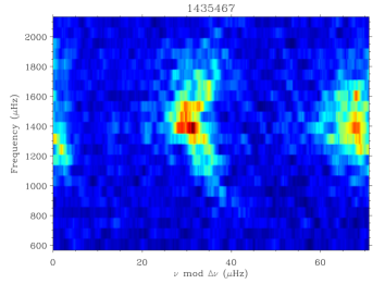
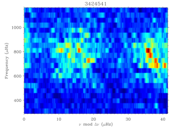
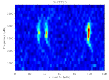
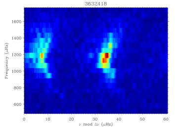
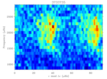
Figure 8: Echelle diagrams of the power spectra of KIC 1435467, KIC 2837475, KIC 3424541, KIC 3427720, KIC 3632418 and KIC 3733735. The power spectra are normalised by the background and then smoothed over 3 $\mu$Hz.

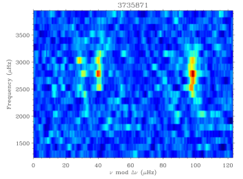
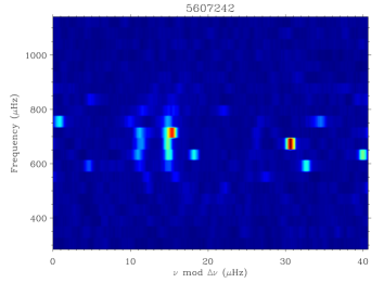
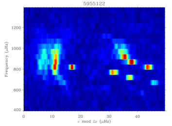
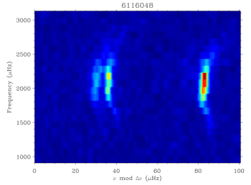
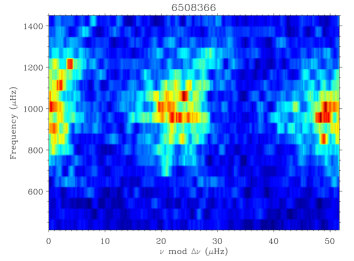
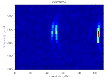
Figure 9: Echelle diagrams of the power spectra of KIC 3735871, KIC 5607242, KIC 5955122, KIC 6116048, KIC 6508366 and KIC 6603624. The power spectra are normalised by the background and then smoothed over 3 $\mu$Hz.

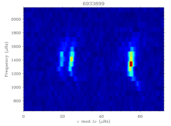
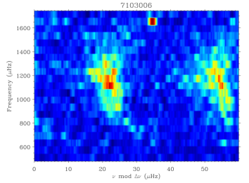
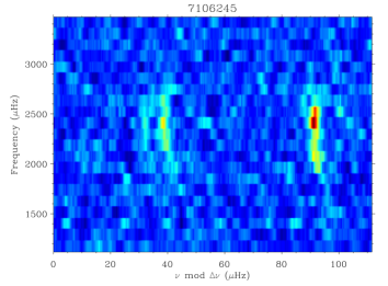
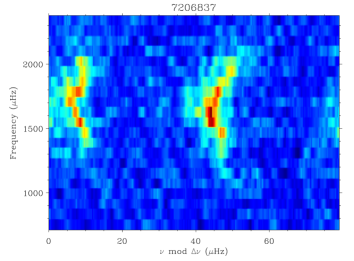
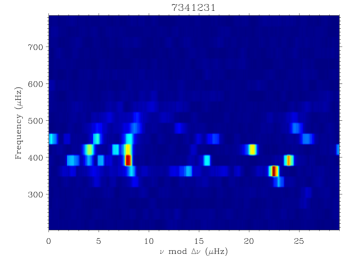
Figure 10: Echelle diagrams of the power spectra of KIC 6679371, KIC 6933899, KIC 7103006, KIC 7106245, KIC 7206837 and KIC 7341231. The power spectra are normalised by the background and then smoothed over 3 $\mu$Hz.

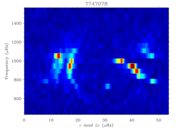
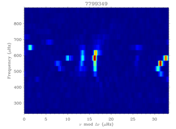
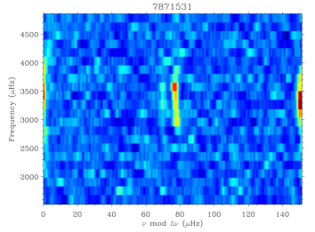
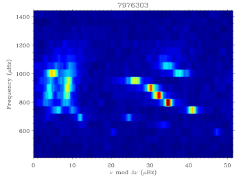
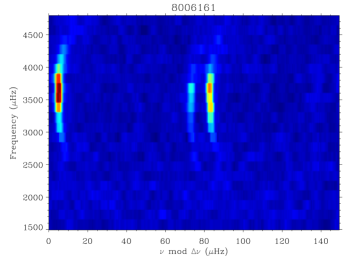
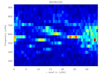
Figure 11: Echelle diagrams of the power spectra of KIC 7747078, KIC 7799349, KIC 7871531, KIC 7976303, KIC 8006161 and KIC 8026226. The power spectra are normalised by the background and then smoothed over 3 $\mu$Hz.

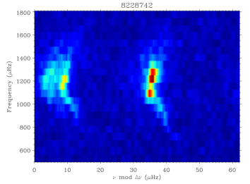
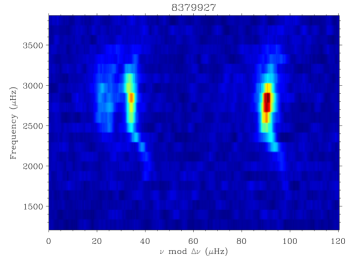
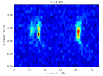
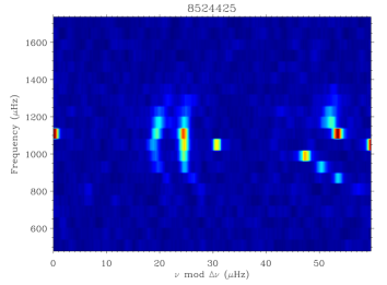
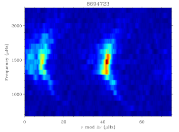
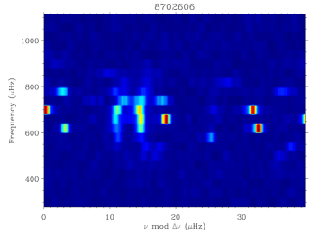
Figure 12: Echelle diagrams of the power spectra of KIC 8228742, KIC 8379927, KIC 8394589, KIC 8524425, KIC 8694723 and KIC 8702606. The power spectra are normalised by the background and then smoothed over 3 $\mu$Hz.

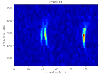
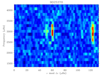
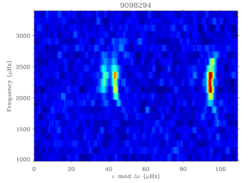
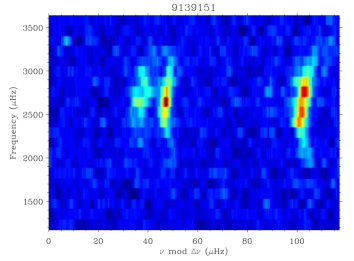
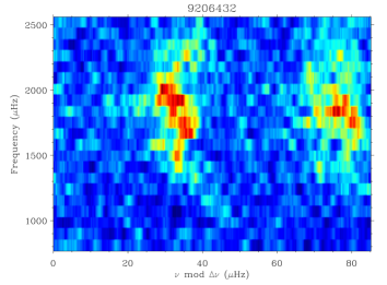
Figure 13: Echelle diagrams of the power spectra of KIC 8760414, KIC 9025370, KIC 9098294, KIC 9139151, KIC 9139163 and KIC 9206432. The power spectra are normalised by the background and then smoothed over 3 $\mu$Hz.

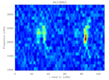
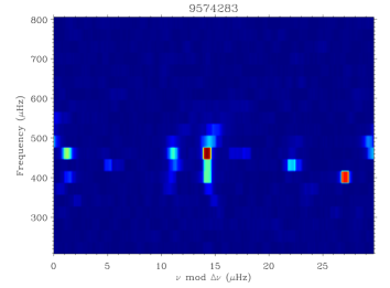
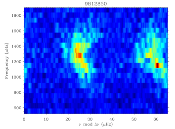
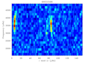
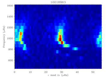
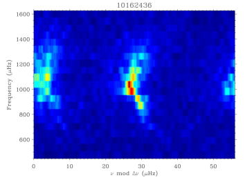
Figure 14: Echelle diagrams of the power spectra of KIC 9410862, KIC 9574283, KIC 9812850, KIC 9955598, KIC 10018963 and KIC 10162436. The power spectra are normalised by the background and then smoothed over 3 $\mu$Hz.

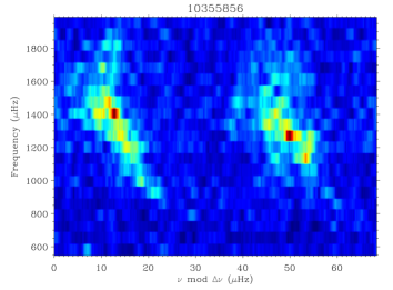
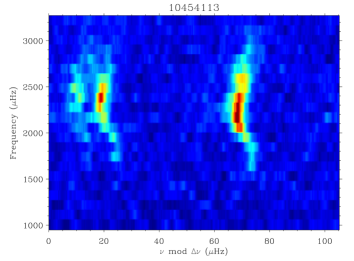
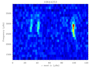
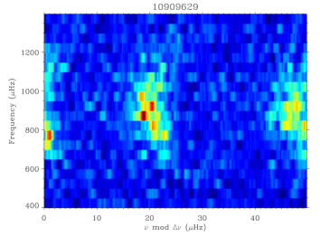
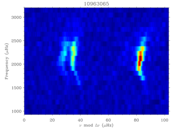
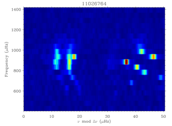
Figure 15: Echelle diagrams of the power spectra of KIC 10355856, KIC 10454113, KIC 10644253, KIC 10909629, KIC 10963065 and KIC 11026764. The power spectra are normalised by the background and then smoothed over 3 $\mu$Hz.

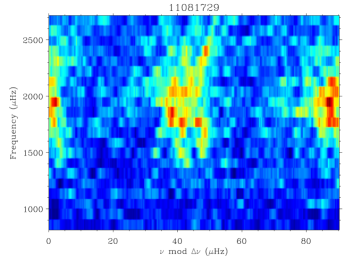
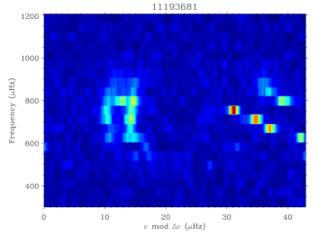
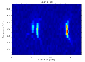
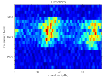
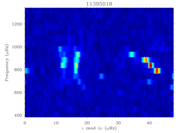
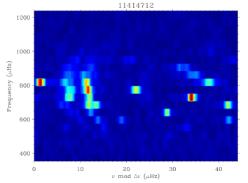
Figure 16: Echelle diagrams of the power spectra of KIC 11081729, KIC 11193681, KIC 11244118, KIC 11253226, KIC 11395018 and KIC 11414712. The power spectra are normalised by the background and then smoothed over 3 $\mu$Hz.

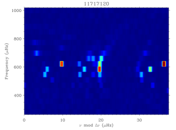
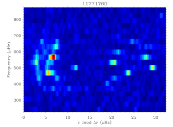
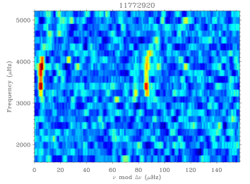
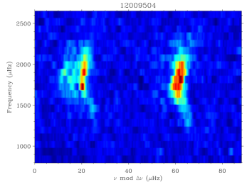
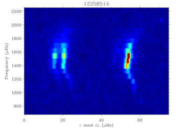
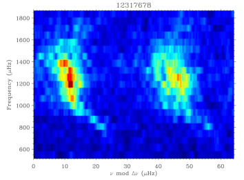
Figure 17: Echelle diagrams of the power spectra of KIC 11717120, KIC 11771760, KIC 11772920, KIC 12009504, KIC 12258514 and KIC 12317678. The power spectra are normalised by the background and then smoothed over 3 $\mu$Hz.

Table 8: Frequencies for KIC 1435467. The first column is the degree. The second column is the frequency. The third column is the 68%-credible interval quoted when the mode is fitted. The last column provides an indication of the quality of the detection: OK indicates that the mode was correctly detected and fitted; Not detected indicates that the mode was fitted but not detected by the quality assurance test and Not fitted indicates that the mode was detected with a posterior probability provided by the quality assurance test. When an uncertainty and a posterior probability are quoted, it means that the mode is fitted but detected using the quality assurance test with a probability lower than 90%.

Degree	Frequency ($\mu$Hz)	68% credible ($\mu$Hz)	Comment
0	992.752	+0.817 / -0.635	OK
0	1064.053	+0.475 / -0.561	OK
0	1135.629	+0.410 / -0.450	OK
0	1206.221	+0.188 / -0.226	OK
0	1274.392	+0.271 / -0.316	OK
0	1344.028	+0.317 / -0.357	OK
0	1414.186	+0.301 / -0.338	OK
0	1485.429	+0.358 / -0.318	OK
0	1556.749	+0.336 / -0.378	OK
0	1626.041	+0.477 / -0.477	OK
0	1698.262	+0.572 / -0.531	OK
0	1770.598	+0.951 / -0.951	OK
0	1842.029	+0.973 / -1.022	OK
0	1912.611	+0.959 / -1.012	OK
0	1983.466	+1.426 / -1.473	OK
1	956.270	Not fitted	0.710
1	1026.739	+0.452 / -0.508	OK
1	1096.903	+0.345 / -0.388	OK
1	1168.054	+0.338 / -0.338	OK
1	1237.866	+0.205 / -0.205	OK
1	1307.203	+0.317 / -0.277	OK
1	1376.074	+0.269 / -0.269	OK
1	1445.906	+0.292 / -0.292	OK
1	1517.838	+0.314 / -0.314	OK
1	1590.530	+0.293 / -0.293	OK
1	1662.385	+0.376 / -0.376	OK
1	1733.286	+0.462 / -0.420	OK
1	1804.266	+0.618 / -0.665	OK
1	1874.800	+0.756 / -0.756	OK
1	1946.806	+0.759 / -0.658	OK
1	2019.615	+0.819 / -0.877	OK
2	989.305	+2.308 / -2.451	OK
2	1059.494	+1.300 / -1.298	OK
2	1129.521	+0.746 / -0.746	OK
2	1199.325	+0.449 / -0.628	OK
2	1268.328	+0.642 / -0.642	OK
2	1338.288	+0.709 / -0.620	OK
2	1408.902	+0.547 / -0.638	OK
2	1480.234	+0.648 / -0.648	OK
2	1551.839	+0.698 / -0.698	OK
2	1623.900	+0.685 / -0.684	OK
2	1695.649	+0.898 / -0.987	OK
2	1766.228	+1.285 / -1.375	OK
2	1836.974	+1.317 / -1.410	OK
2	1907.883	+1.362 / -1.452	OK
2	1979.145	+2.073 / -2.259	OK

Table 9: Frequencies for KIC 2837475. The first column is the degree. The second column is the frequency. The third column is the 68%-credible interval quoted when the mode is fitted. The last column provides an indication of the quality of the detection: OK indicates that the mode was correctly detected and fitted; Not detected indicates that the mode was fitted but not detected by the quality assurance test and Not fitted indicates that the mode was detected with a posterior probability provided by the quality assurance test. When an uncertainty and a posterior probability are quoted, it means that the mode is fitted but detected using the quality assurance test with a probability lower than 90%.

Degree	Frequency ($\mu$Hz)	68% credible ($\mu$Hz)	Comment
0	985.740	+0.169 / -0.225	OK
0	1057.562	+0.842 / -0.841	OK
0	1130.442	+0.702 / -0.654	OK
0	1205.403	+0.547 / -0.638	OK
0	1279.772	+0.674 / -0.674	OK
0	1355.167	+0.515 / -0.566	OK
0	1432.082	+0.514 / -0.608	OK
0	1509.488	+0.409 / -0.368	OK
0	1585.937	+0.484 / -0.537	OK
0	1660.125	+0.631 / -0.631	OK
0	1734.503	+0.654 / -0.654	OK
0	1810.869	+0.946 / -0.946	OK
0	1886.532	+1.081 / -1.029	OK
0	1963.679	+1.459 / -1.400	OK
0	2041.304	+2.430 / -2.246	OK
0	2117.550	Not fitted	0.630
0	2194.480	Not fitted	0.813
0	2265.410	Not fitted	0.807
1	1020.321	+0.258 / -0.309	OK
1	1093.727	+0.617 / -0.566	OK
1	1167.088	+0.578 / -0.525	OK
1	1241.065	+0.532 / -0.577	OK
1	1315.382	+0.654 / -0.653	OK
1	1390.946	+0.467 / -0.467	OK
1	1468.287	+0.518 / -0.518	OK
1	1544.878	+0.431 / -0.431	OK
1	1620.036	+0.467 / -0.513	OK
1	1695.664	+0.432 / -0.432	OK
1	1771.638	+0.523 / -0.522	OK
1	1845.982	+0.607 / -0.560	OK
1	1922.405	+0.686 / -0.686	OK
1	2000.119	+0.770 / -0.770	OK
1	2077.552	+1.182 / -1.128	OK
1	2303.520	Not fitted	0.855
2	977.959	+4.691 / -3.024	Not detected
2	1051.458	+3.784 / -1.258	OK
2	1125.882	+1.897 / -1.624	OK
2	1199.526	+1.111 / -1.295	OK
2	1272.976	+1.124 / -1.123	OK
2	1347.530	+1.152 / -1.151	OK
2	1423.080	+1.222 / -1.119	OK
2	1499.386	+1.509 / -1.407	OK
2	1575.939	+1.865 / -1.569	OK
2	1652.855	+2.032 / -2.029	OK
2	1729.308	+2.131 / -2.128	OK
2	1805.913	+1.800 / -1.893	OK
2	1882.285	+1.280 / -1.377	OK
2	1959.293	+1.425 / -1.526	OK
2	2036.156	+2.423 / -2.630	OK
2	2265.410	Not fitted	0.807

Table 10: Frequencies for KIC 3424541. The first column is the degree. The second column is the frequency. The third column is the 68%-credible interval quoted when the mode is fitted. The last column provides an indication of the quality of the detection: OK indicates that the mode was correctly detected and fitted; Not detected indicates that the mode was fitted but not detected by the quality assurance test and Not fitted indicates that the mode was detected with a posterior probability provided by the quality assurance test. When an uncertainty and a posterior probability are quoted, it means that the mode is fitted but detected using the quality assurance test with a probability lower than 90%.

Degree	Frequency ($\mu$Hz)	68% credible ($\mu$Hz)	Comment
0	515.159	+0.898 / -0.998	OK
0	554.896	+0.750 / -0.847	OK
0	594.851	+0.832 / -0.964	OK
0	635.872	+0.854 / -1.029	OK
0	677.707	+0.631 / -0.664	OK
0	720.542	+0.430 / -0.460	OK
0	761.406	+0.617 / -0.644	OK
0	801.236	+0.460 / -0.521	OK
0	842.571	+0.716 / -0.751	OK
0	884.695	+0.676 / -0.675	OK
0	926.904	+0.674 / -0.704	OK
0	966.729	+0.432 / -0.432	OK
0	1008.191	+1.030 / -1.065	OK
0	1049.754	+1.868 / -2.146	Not detected
0	1092.100	Not fitted	0.867
1	368.423	Not fitted	0.663
1	497.417	+0.413 / -0.461	0.703
1	535.467	+0.548 / -0.547	OK
1	574.884	+0.510 / -0.537	OK
1	616.271	+0.583 / -0.583	OK
1	659.448	+0.457 / -0.483	OK
1	699.337	+0.372 / -0.338	OK
1	740.189	+0.390 / -0.420	OK
1	781.366	+0.478 / -0.478	OK
1	821.304	+0.494 / -0.467	OK
1	863.283	+0.564 / -0.531	OK
1	906.191	+0.586 / -0.553	OK
1	948.677	+0.583 / -0.582	OK
1	990.946	+0.423 / -0.455	OK
1	1032.211	+0.785 / -0.941	Not detected
1	1070.390	Not fitted	0.825
1	1115.410	Not fitted	0.870
2	510.044	+1.390 / -1.142	Not detected
2	549.930	+1.048 / -0.994	OK
2	590.101	+1.087 / -0.930	OK
2	631.710	+0.911 / -0.910	OK
2	673.375	+0.930 / -0.878	OK
2	714.813	+0.885 / -0.785	OK
2	755.444	+0.775 / -0.774	OK
2	796.314	+0.838 / -0.732	OK
2	837.143	+1.043 / -1.042	OK
2	878.519	+1.377 / -1.222	OK
2	920.884	+1.426 / -1.319	OK
2	963.606	+1.182 / -1.227	OK
2	1005.239	+1.464 / -1.406	OK
2	1046.639	+2.249 / -2.195	Not detected

Table 11: Frequencies for KIC 3427720. The first column is the degree. The second column is the frequency. The third column is the 1-$\sigma$ uncertainty quoted when the mode is fitted. The last column provides an indication of the quality of the detection: OK indicates that the mode was correctly detected and fitted; Not detected indicates that the mode was fitted but not detected by the quality assurance test and Not fitted indicates that the mode was detected with a posterior probability provided by the quality assurance test. When an uncertainty and a posterior probability are quoted, it means that the mode is fitted but detected using the quality assurance test with a probability lower than 90%.

Degree	Frequency ($\mu$Hz)	1-$\sigma$ error ($\mu$Hz)	Comment
0	2207.437	0.631	OK
0	2325.063	0.244	OK
0	2444.427	0.280	OK
0	2564.300	0.218	OK
0	2684.764	0.143	OK
0	2804.640	0.328	OK
0	2925.244	0.361	OK
0	3044.276	0.396	OK
0	3165.060	0.541	Not detected
0	3287.661	0.293	0.866
1	2024.400	Not fitted	0.706
1	2144.016	0.453	OK
1	2262.339	0.244	OK
1	2380.617	0.285	OK
1	2500.464	0.206	OK
1	2621.039	0.160	OK
1	2741.644	0.206	OK
1	2861.405	0.186	OK
1	2981.503	0.264	OK
1	3101.854	0.289	OK
1	3223.454	0.395	Not detected
2	2195.406	0.619	OK
2	2314.163	0.365	OK
2	2433.841	0.259	OK
2	2553.282	0.328	OK
2	2674.781	0.197	OK
2	2793.974	0.383	OK
2	2914.192	0.419	OK
2	3034.861	0.484	OK
2	3156.454	0.667	0.859
2	3278.512	0.748	Not detected

Table 12: Frequencies for KIC 3632418. The first column is the degree. The second column is the frequency. The third column is the 1-$\sigma$ uncertainty quoted when the mode is fitted. The last column provides an indication of the quality of the detection: OK indicates that the mode was correctly detected and fitted; Not detected indicates that the mode was fitted but not detected by the quality assurance test and Not fitted indicates that the mode was detected with a posterior probability provided by the quality assurance test. When an uncertainty and a posterior probability are quoted, it means that the mode is fitted but detected using the quality assurance test with a probability lower than 90%.

Degree	Frequency ($\mu$Hz)	1-$\sigma$ error ($\mu$Hz)	Comment
0	682.388	Not fitted	0.709
0	740.494	Not fitted	0.694
0	799.280	0.410	OK
0	858.930	0.240	OK
0	920.370	0.180	OK
0	979.300	0.160	OK
0	1039.310	0.190	OK
0	1099.260	0.180	OK
0	1159.920	0.180	OK
0	1221.310	0.200	OK
0	1282.550	0.200	OK
0	1342.600	0.400	OK
0	1405.040	0.250	OK
0	1464.790	0.570	OK
0	1645.870	Not fitted	0.861
1	709.051	Not fitted	0.666
1	765.354	Not fitted	0.658
1	824.590	0.420	OK
1	885.250	0.190	OK
1	946.450	0.180	OK
1	1006.170	0.180	OK
1	1065.010	0.160	OK
1	1125.860	0.140	OK
1	1186.780	0.150	OK
1	1248.100	0.180	OK
1	1309.960	0.140	OK
1	1370.890	0.200	OK
1	1432.220	0.200	OK
1	1493.980	0.260	OK
1	1612.500	Not fitted	0.831
2	682.388	Not fitted	0.709
2	740.494	Not fitted	0.694
2	916.940	0.430	OK
2	976.340	0.290	OK
2	1034.990	0.370	OK
2	1094.420	0.270	OK
2	1155.090	0.210	OK
2	1217.370	0.350	OK
2	1277.980	0.190	OK
2	1342.420	0.460	OK
2	1400.910	0.480	OK
2	1460.440	0.760	OK
2	1574.440	Not fitted	0.576

Table 13: Frequencies for KIC 3733735. The first column is the degree. The second column is the frequency. The third column is the 68%-credible interval quoted when the mode is fitted. The last column provides an indication of the quality of the detection: OK indicates that the mode was correctly detected and fitted; Not detected indicates that the mode was fitted but not detected by the quality assurance test and Not fitted indicates that the mode was detected with a posterior probability provided by the quality assurance test. When an uncertainty and a posterior probability are quoted, it means that the mode is fitted but detected using the quality assurance test with a probability lower than 90%.

Degree	Frequency ($\mu$Hz)	68% credible ($\mu$Hz)	Comment
0	1207.275	+1.933 / -1.999	Not detected
0	1296.993	+0.663 / -0.783	0.701
0	1386.418	+0.877 / -0.877	OK
0	1475.046	+0.780 / -0.780	OK
0	1564.659	+1.051 / -1.050	OK
0	1655.392	+0.545 / -0.600	OK
0	1746.599	+0.543 / -0.603	OK
0	1840.152	+0.776 / -0.711	OK
0	1934.770	+0.679 / -0.740	OK
0	2027.616	+0.839 / -0.903	OK
0	2118.940	+0.583 / -0.636	OK
0	2210.372	+0.826 / -0.894	OK
0	2301.778	+0.968 / -0.887	OK
0	2394.698	+0.882 / -0.882	OK
0	2487.872	+0.573 / -0.516	OK
0	2580.729	+1.731 / -1.730	OK
0	2761.700	Not fitted	0.867
0	2947.460	Not fitted	0.852
1	1158.006	+4.157 / -4.060	Not detected
1	1247.271	+2.149 / -2.231	Not detected
1	1336.416	+0.843 / -0.702	OK
1	1425.981	+0.851 / -0.773	OK
1	1515.171	+0.726 / -0.726	OK
1	1605.189	+0.782 / -0.726	OK
1	1695.891	+0.411 / -0.411	OK
1	1788.845	+0.553 / -0.553	OK
1	1882.074	+0.528 / -0.587	OK
1	1974.958	+0.571 / -0.571	OK
1	2068.381	+0.745 / -0.687	OK
1	2161.319	+0.481 / -0.549	OK
1	2254.070	+0.808 / -0.943	OK
1	2346.065	+1.117 / -1.116	OK
1	2437.515	+1.117 / -1.037	OK
1	2527.773	+0.630 / -0.567	OK
1	2618.528	+1.887 / -1.886	OK
2	1193.353	+5.465 / -5.133	Not detected
2	1282.766	+3.751 / -3.313	Not detected
2	1372.137	+2.820 / -2.229	OK
2	1462.461	+2.444 / -2.196	OK
2	1553.355	+2.556 / -2.284	OK
2	1645.004	+2.644 / -2.869	OK
2	1737.415	+2.676 / -3.717	OK
2	1830.877	+2.560 / -3.485	OK
2	1924.991	+1.979 / -3.212	OK
2	2018.465	+1.808 / -2.322	OK
2	2110.910	+1.605 / -1.604	OK
2	2203.185	+1.356 / -1.232	OK
2	2295.285	+1.506 / -1.505	OK
2	2388.019	+1.858 / -1.972	OK
2	2480.757	+2.167 / -3.092	OK
2	2573.191	+3.271 / -4.828	OK
2	2932.240	Not fitted	0.863

Table 14: Frequencies for KIC 3735871. The first column is the degree. The second column is the frequency. The third column is the 68%-credible interval quoted when the mode is fitted. The last column provides an indication of the quality of the detection: OK indicates that the mode was correctly detected and fitted; Not detected indicates that the mode was fitted but not detected by the quality assurance test and Not fitted indicates that the mode was detected with a posterior probability provided by the quality assurance test. When an uncertainty and a posterior probability are quoted, it means that the mode is fitted but detected using the quality assurance test with a probability lower than 90%.

Degree	Frequency ($\mu$Hz)	68% credible ($\mu$Hz)	Comment
0	2247.640	Not fitted	0.614
0	2375.005	+0.760 / -0.859	OK
0	2500.882	+0.293 / -0.312	OK
0	2624.587	+0.190 / -0.196	OK
0	2746.938	+0.289 / -0.289	OK
0	2870.265	+0.527 / -0.596	OK
0	2993.256	+0.331 / -0.331	OK
0	3117.781	+0.370 / -0.358	OK
0	3244.134	+0.695 / -0.918	Not detected
0	3369.276	+1.520 / -1.814	Not detected
0	3494.141	+2.348 / -3.233	Not detected
0	3618.881	+3.662 / -4.980	Not detected
1	1927.430	Not fitted	0.572
1	2056.550	Not fitted	0.695
1	2300.500	Not fitted	0.600
1	2314.535	+0.538 / -0.651	OK
1	2436.561	+0.283 / -0.310	OK
1	2558.186	+0.251 / -0.251	OK
1	2681.946	+0.156 / -0.156	OK
1	2805.076	+0.338 / -0.329	OK
1	2926.893	+0.447 / -0.371	OK
1	3050.760	+0.470 / -0.459	OK
1	3175.231	+0.545 / -0.616	OK
1	3299.693	+0.827 / -0.882	0.696
1	3424.191	+2.375 / -2.476	Not detected
1	3548.722	+4.463 / -4.626	Not detected
2	1981.510	Not fitted	0.710
2	2366.009	+1.703 / -1.624	OK
2	2489.364	+0.989 / -0.840	OK
2	2613.201	+1.005 / -0.978	OK
2	2737.463	+0.316 / -0.334	OK
2	2859.516	+1.401 / -1.050	OK
2	2981.966	+0.631 / -0.463	OK
2	3105.303	+0.745 / -0.745	OK
2	3229.273	+1.004 / -1.004	Not detected
2	3354.202	+1.130 / -1.554	Not detected
2	3479.350	+2.614 / -3.242	Not detected
2	3604.491	+4.686 / -5.399	Not detected

Table 15: Frequencies for KIC 5607242. The first column is the degree. The second column is the frequency. The third column is the 1-$\sigma$ uncertainty quoted when the mode is fitted. The last column provides an indication of the quality of the detection: OK indicates that the mode was correctly detected and fitted; Not detected indicates that the mode was fitted but not detected by the quality assurance test and Not fitted indicates that the mode was detected with a posterior probability provided by the quality assurance test. When an uncertainty and a posterior probability are quoted, it means that the mode is fitted but detected using the quality assurance test with a probability lower than 90%.

Degree	Frequency ($\mu$Hz)	1-$\sigma$ error ($\mu$Hz)	Comment
0	504.104	0.032	OK
0	543.376	0.090	OK
0	583.050	0.076	OK
0	623.645	0.045	OK
0	664.119	0.049	OK
0	704.801	0.098	OK
0	745.287	0.084	OK
0	786.310	0.156	OK
0	827.058	0.264	OK
0	868.990	0.811	OK
1	371.818	Not fitted	0.622
1	467.697	Not fitted	0.709
1	485.242	0.343	OK
1	509.017	0.031	OK
1	527.565	0.034	OK
1	554.995	0.129	OK
1	572.791	0.089	OK
1	600.775	0.061	OK
1	626.905	0.055	OK
1	648.623	0.059	OK
1	679.921	0.037	OK
1	705.359	0.076	OK
1	731.227	0.075	OK
1	764.822	0.104	OK
1	792.989	0.145	OK
1	816.677	0.150	OK
1	851.846	0.286	OK
1	889.136	0.730	0.868
1	923.697	Not fitted	0.853
2	499.255	0.013	OK
2	539.702	0.132	OK
2	579.354	0.086	OK
2	619.687	0.047	OK
2	660.523	0.071	OK
2	701.137	0.062	OK
2	740.434	0.133	OK
2	782.653	0.145	OK
2	824.289	0.365	OK
2	866.243	3.016	OK
3	675.487	0.157	OK
3	716.263	0.138	OK
3	757.426	0.458	OK

Table 16: Frequencies for KIC 5955122. The first column is the degree. The second column is the frequency. The third column is the 1-$\sigma$ uncertainty quoted when the mode is fitted. The last column provides an indication of the quality of the detection: OK indicates that the mode was correctly detected and fitted; Not detected indicates that the mode was fitted but not detected by the quality assurance test and Not fitted indicates that the mode was detected with a posterior probability provided by the quality assurance test. When an uncertainty and a posterior probability are quoted, it means that the mode is fitted but detected using the quality assurance test with a probability lower than 90%.

Degree	Frequency ($\mu$Hz)	1-$\sigma$ error ($\mu$Hz)	Comment
0	508.907	Not fitted	0.561
0	561.117	0.259	OK
0	609.718	0.163	OK
0	658.498	0.355	OK
0	706.164	0.194	OK
0	754.359	0.126	OK
0	803.714	0.093	OK
0	853.473	0.123	OK
0	903.104	0.151	OK
0	952.668	0.191	OK
0	1002.451	0.263	OK
0	1052.268	0.416	OK
0	1104.737	0.639	OK
0	1155.150	Not fitted	0.850
1	508.907	Not fitted	0.561
1	574.827	0.231	OK
1	586.344	0.144	OK
1	623.587	0.340	OK
1	632.632	0.217	OK
1	657.474	0.282	OK
1	690.112	0.141	OK
1	731.011	0.130	OK
1	774.916	0.106	OK
1	809.729	0.144	OK
1	836.646	0.094	OK
1	880.086	0.124	OK
1	927.117	0.140	OK
1	975.990	0.189	OK
1	1025.152	0.241	OK
1	1073.686	0.337	OK
1	1119.196	0.381	OK
1	1155.150	Not fitted	0.850
1	1230.280	Not fitted	0.673
2	653.068	0.350	OK
2	701.490	0.344	OK
2	749.720	0.253	OK
2	799.480	0.148	OK
2	849.042	0.183	OK
2	898.478	0.250	OK
2	948.528	0.323	OK
2	997.886	0.396	OK
2	1047.614	0.738	OK
2	1097.643	0.705	OK
2	1146.390	Not fitted	0.805

Table 17: Frequencies for KIC 6116048. The first column is the degree. The second column is the frequency. The third column is the 1-$\sigma$ uncertainty quoted when the mode is fitted. The last column provides an indication of the quality of the detection: OK indicates that the mode was correctly detected and fitted; Not detected indicates that the mode was fitted but not detected by the quality assurance test and Not fitted indicates that the mode was detected with a posterior probability provided by the quality assurance test. When an uncertainty and a posterior probability are quoted, it means that the mode is fitted but detected using the quality assurance test with a probability lower than 90%.

Degree	Frequency ($\mu$Hz)	1-$\sigma$ error ($\mu$Hz)	Comment
0	1550.390	0.160	OK
0	1649.830	0.150	OK
0	1748.080	0.140	OK
0	1847.980	0.130	OK
0	1948.290	0.110	OK
0	2049.460	0.130	OK
0	2149.990	0.110	OK
0	2250.410	0.150	OK
0	2352.280	0.260	OK
0	2452.990	0.240	OK
0	2554.950	0.610	OK
0	2658.100	Not fitted	0.834
0	2753.350	Not fitted	0.819
0	2856.990	Not fitted	0.822
1	1393.700	Not fitted	0.694
1	1494.980	0.260	OK
1	1595.300	0.200	OK
1	1694.420	0.150	OK
1	1793.340	0.150	OK
1	1893.950	0.110	OK
1	1995.150	0.100	OK
1	2096.030	0.110	OK
1	2196.690	0.110	OK
1	2298.040	0.150	OK
1	2399.210	0.190	OK
1	2501.850	0.300	OK
1	2604.150	0.490	OK
1	2703.760	Not fitted	0.863
2	1342.680	Not fitted	0.699
2	1543.300	0.590	OK
2	1642.530	0.530	OK
2	1741.440	0.340	OK
2	1841.140	0.150	OK
2	1941.650	0.140	OK
2	2043.370	0.160	OK
2	2143.880	0.150	OK
2	2245.240	0.240	OK
2	2346.010	0.410	OK
2	2448.300	0.780	OK
2	2551.400	1.740	OK
2	2753.350	Not fitted	0.819

Table 18: Frequencies for KIC 6508366. The first column is the degree. The second column is the frequency. The third column is the 68%-credible interval quoted when the mode is fitted. The last column provides an indication of the quality of the detection: OK indicates that the mode was correctly detected and fitted; Not detected indicates that the mode was fitted but not detected by the quality assurance test and Not fitted indicates that the mode was detected with a posterior probability provided by the quality assurance test. When an uncertainty and a posterior probability are quoted, it means that the mode is fitted but detected using the quality assurance test with a probability lower than 90%.

Degree	Frequency ($\mu$Hz)	68% credible ($\mu$Hz)	Comment
0	622.782	+0.586 / -0.586	0.704
0	672.204	+0.629 / -0.629	OK
0	722.846	+0.445 / -0.445	OK
0	775.109	+0.294 / -0.324	OK
0	826.341	+0.341 / -0.341	OK
0	877.627	+0.341 / -0.341	OK
0	928.955	+0.392 / -0.392	OK
0	979.470	+0.429 / -0.400	OK
0	1030.870	+0.286 / -0.314	OK
0	1083.772	+0.429 / -0.400	OK
0	1137.175	+0.401 / -0.400	OK
0	1189.993	+0.381 / -0.413	OK
0	1241.728	+0.608 / -0.608	OK
0	1293.248	+0.802 / -0.768	OK
0	1345.443	+1.359 / -1.402	OK
0	1394.910	Not fitted	0.852
1	596.156	+1.169 / -1.133	Not detected
1	645.356	+0.600 / -0.567	OK
1	694.004	+0.391 / -0.423	OK
1	744.731	+0.382 / -0.411	OK
1	796.168	+0.326 / -0.293	OK
1	848.680	+0.351 / -0.324	OK
1	901.024	+0.314 / -0.314	OK
1	951.267	+0.278 / -0.250	OK
1	1002.882	+0.271 / -0.301	OK
1	1054.058	+0.264 / -0.234	OK
1	1107.459	+0.323 / -0.294	OK
1	1159.366	+0.452 / -0.422	OK
1	1212.665	+0.476 / -0.476	OK
1	1265.253	+0.485 / -0.447	OK
1	1317.549	+0.818 / -0.818	OK
1	1371.172	+1.547 / -1.596	OK
1	1422.500	Not fitted	0.871
1	1471.300	Not fitted	0.634
2	618.025	+2.549 / -2.739	Not detected
2	668.970	+1.476 / -1.807	OK
2	719.958	+1.153 / -1.079	OK
2	771.570	+0.660 / -0.733	OK
2	823.269	+0.579 / -0.506	OK
2	874.571	+0.573 / -0.573	OK
2	925.154	+0.770 / -0.770	OK
2	976.915	+0.698 / -0.837	OK
2	1028.317	+0.543 / -0.543	OK
2	1080.846	+0.589 / -0.588	OK
2	1133.837	+0.642 / -0.641	OK
2	1186.441	+0.734 / -0.660	OK
2	1237.987	+0.826 / -0.756	OK
2	1289.505	+0.993 / -1.054	OK
2	1341.134	+1.950 / -2.103	OK
2	1489.910	Not fitted	0.579

Table 19: Frequencies for KIC 6603624. The first column is the degree. The second column is the frequency. The third column is the 1-$\sigma$ uncertainty quoted when the mode is fitted. The last column provides an indication of the quality of the detection: OK indicates that the mode was correctly detected and fitted; Not detected indicates that the mode was fitted but not detected by the quality assurance test and Not fitted indicates that the mode was detected with a posterior probability provided by the quality assurance test. When an uncertainty and a posterior probability are quoted, it means that the mode is fitted but detected using the quality assurance test with a probability lower than 90%.

Degree	Frequency ($\mu$Hz)	1-$\sigma$ error ($\mu$Hz)	Comment
0	1819.570	0.120	OK
0	1928.480	0.140	OK
0	2036.940	0.070	OK
0	2146.780	0.070	OK
0	2256.960	0.090	OK
0	2367.050	0.060	OK
0	2477.100	0.070	OK
0	2587.510	0.080	OK
0	2698.360	0.170	OK
0	2806.710	0.950	OK
0	3028.490	Not fitted	0.861
1	1760.530	0.110	OK
1	1869.750	0.110	OK
1	1978.720	0.140	OK
1	2088.330	0.050	OK
1	2198.460	0.070	OK
1	2309.010	0.050	OK
1	2419.470	0.060	OK
1	2529.730	0.070	OK
1	2640.460	0.090	OK
1	2751.160	0.080	OK
1	2862.450	0.620	OK
1	2974.460	Not fitted	0.871
2	1812.780	0.110	OK
2	1921.720	0.180	OK
2	2030.900	0.130	OK
2	2141.040	0.090	OK
2	2251.610	0.070	OK
2	2362.080	0.050	OK
2	2472.460	0.100	OK
2	2583.100	0.080	OK
2	2693.980	0.100	OK
2	2806.710	1.890	OK
2	3028.490	Not fitted	0.861

Table 20: Frequencies for KIC 6679371. The first column is the degree. The second column is the frequency. The third column is the 68%-credible interval quoted when the mode is fitted. The last column provides an indication of the quality of the detection: OK indicates that the mode was correctly detected and fitted; Not detected indicates that the mode was fitted but not detected by the quality assurance test and Not fitted indicates that the mode was detected with a posterior probability provided by the quality assurance test. When an uncertainty and a posterior probability are quoted, it means that the mode is fitted but detected using the quality assurance test with a probability lower than 90%.

Degree	Frequency ($\mu$Hz)	68% credible ($\mu$Hz)	Comment
0	298.997	Not fitted	0.569
0	555.363	+1.167 / -1.209	Not detected
0	606.509	+0.301 / -0.335	0.697
0	656.927	+0.387 / -0.457	OK
0	704.583	+0.492 / -0.527	OK
0	752.698	+0.420 / -0.455	OK
0	803.166	+0.301 / -0.334	OK
0	854.637	+0.273 / -0.273	OK
0	904.941	+0.228 / -0.228	OK
0	956.589	+0.294 / -0.326	OK
0	1007.842	+0.301 / -0.301	OK
0	1057.374	+0.458 / -0.425	OK
0	1106.851	+0.447 / -0.479	OK
0	1157.878	+0.622 / -0.621	OK
0	1209.282	+0.446 / -0.480	OK
0	1262.380	+0.537 / -0.536	OK
0	1313.877	+0.834 / -0.794	OK
0	1365.205	+0.938 / -0.871	OK
0	1417.344	+1.363 / -1.322	OK
0	1465.930	Not fitted	0.861
0	1527.010	Not fitted	0.843
1	577.997	+0.337 / -0.412	0.693
1	628.633	+0.319 / -0.319	OK
1	677.564	+0.343 / -0.342	OK
1	725.750	+0.286 / -0.250	OK
1	774.772	+0.335 / -0.335	OK
1	825.029	+0.243 / -0.243	OK
1	876.900	+0.309 / -0.278	OK
1	928.205	+0.253 / -0.253	OK
1	978.385	+0.255 / -0.255	OK
1	1028.600	+0.276 / -0.241	OK
1	1079.790	+0.326 / -0.326	OK
1	1129.762	+0.392 / -0.360	OK
1	1181.655	+0.408 / -0.408	OK
1	1234.010	+0.476 / -0.515	OK
1	1284.774	+0.501 / -0.468	OK
1	1336.540	+0.694 / -0.693	OK
1	1389.323	+0.631 / -0.586	OK
1	1442.837	+0.833 / -0.885	OK
1	1492.930	Not fitted	0.856
1	1653.830	Not fitted	0.865
2	550.249	+0.548 / -1.149	Not detected
2	599.852	+0.781 / -0.851	Not detected
2	649.285	+0.712 / -0.711	OK
2	698.002	+0.749 / -0.686	OK
2	747.779	+0.969 / -0.774	OK
2	799.343	+0.773 / -0.772	OK
2	851.598	+0.640 / -0.639	OK
2	902.103	+0.563 / -0.633	OK
2	951.708	+0.640 / -0.703	OK
2	1002.033	+0.694 / -0.624	OK
2	1053.508	+0.589 / -0.655	OK
2	1104.216	+0.702 / -0.766	OK
2	1155.486	+0.744 / -0.811	OK
2	1207.218	+0.770 / -0.770	OK
2	1259.383	+0.918 / -0.983	OK
2	1311.287	+1.016 / -1.015	OK
2	1362.461	+1.138 / -1.137	OK
2	1413.792	+1.846 / -1.914	OK
2	1465.930	Not fitted	0.861

Table 21: Frequencies for KIC 6933899. The first column is the degree. The second column is the frequency. The third column is the 1-$\sigma$ uncertainty quoted when the mode is fitted. The last column provides an indication of the quality of the detection: OK indicates that the mode was correctly detected and fitted; Not detected indicates that the mode was fitted but not detected by the quality assurance test and Not fitted indicates that the mode was detected with a posterior probability provided by the quality assurance test. When an uncertainty and a posterior probability are quoted, it means that the mode is fitted but detected using the quality assurance test with a probability lower than 90%.

Degree	Frequency ($\mu$Hz)	1-$\sigma$ error ($\mu$Hz)	Comment
0	965.310	0.200	OK
0	1036.720	0.160	OK
0	1107.750	0.170	OK
0	1177.640	0.070	OK
0	1249.050	0.100	OK
0	1321.660	0.110	OK
0	1393.940	0.090	OK
0	1466.220	0.110	OK
0	1538.170	0.100	OK
0	1610.740	0.310	OK
0	1683.510	0.650	OK
0	1756.380	Not fitted	0.853
0	1830.710	Not fitted	0.814
1	853.349	Not fitted	0.705
1	996.190	0.130	OK
1	1067.540	0.080	OK
1	1137.320	0.050	OK
1	1208.220	0.090	OK
1	1279.930	0.100	OK
1	1352.410	0.080	OK
1	1424.560	0.110	OK
1	1496.640	0.120	OK
1	1569.120	0.070	OK
1	1641.110	0.190	OK
1	1714.790	0.500	OK
1	1787.650	Not fitted	0.870
1	1856.360	Not fitted	0.732
2	961.410	0.250	OK
2	1032.190	0.350	OK
2	1101.520	0.370	OK
2	1172.450	0.170	OK
2	1243.480	0.080	OK
2	1316.700	0.120	OK
2	1389.070	0.140	OK
2	1460.900	0.100	OK
2	1533.630	0.160	OK
2	1606.220	0.310	OK
2	1679.560	0.960	OK
2	1756.380	Not fitted	0.853
2	1830.710	Not fitted	0.814

Table 22: Frequencies for KIC 7103006. The first column is the degree. The second column is the frequency. The third column is the 68%-credible interval quoted when the mode is fitted. The last column provides an indication of the quality of the detection: OK indicates that the mode was correctly detected and fitted; Not detected indicates that the mode was fitted but not detected by the quality assurance test and Not fitted indicates that the mode was detected with a posterior probability provided by the quality assurance test. When an uncertainty and a posterior probability are quoted, it means that the mode is fitted but detected using the quality assurance test with a probability lower than 90%.

Degree	Frequency ($\mu$Hz)	68% credible ($\mu$Hz)	Comment
0	654.507	Not fitted	0.703
0	722.230	+0.332 / -0.295	OK
0	779.406	+0.210 / -0.210	OK
0	835.967	+0.250 / -0.250	OK
0	894.308	+0.206 / -0.206	OK
0	954.831	+0.334 / -0.334	OK
0	1014.741	+0.293 / -0.293	OK
0	1073.733	+0.257 / -0.257	OK
0	1132.806	+0.288 / -0.320	OK
0	1191.865	+0.367 / -0.330	OK
0	1251.640	+0.372 / -0.372	OK
0	1311.689	+0.496 / -0.523	OK
0	1372.332	+0.716 / -0.754	OK
0	1432.079	+0.647 / -0.588	OK
0	1493.964	+0.758 / -0.757	OK
0	1556.446	+0.824 / -0.782	OK
0	1620.231	+1.333 / -1.378	OK
0	1674.000	Not fitted	0.867
1	633.713	Not fitted	0.698
1	693.045	+1.431 / -1.389	OK
1	748.872	+0.232 / -0.283	OK
1	804.302	+0.228 / -0.199	OK
1	862.204	+0.235 / -0.235	OK
1	921.588	+0.213 / -0.213	OK
1	980.934	+0.266 / -0.240	OK
1	1041.136	+0.323 / -0.323	OK
1	1100.874	+0.240 / -0.266	OK
1	1159.107	+0.240 / -0.266	OK
1	1218.379	+0.321 / -0.320	OK
1	1279.409	+0.385 / -0.360	OK
1	1339.755	+0.353 / -0.382	OK
1	1400.431	+0.645 / -0.611	OK
1	1459.991	+0.606 / -0.646	OK
1	1521.031	+0.726 / -0.686	OK
1	1584.351	+0.770 / -0.924	OK
1	1710.390	Not fitted	0.854
2	654.507	Not fitted	0.703
2	714.286	+3.623 / -2.797	OK
2	773.211	+2.247 / -1.160	OK
2	832.655	+0.692 / -0.846	OK
2	891.692	+0.958 / -0.877	OK
2	950.164	+0.674 / -0.589	OK
2	1009.253	+0.665 / -0.665	OK
2	1067.324	+0.756 / -0.604	OK
2	1126.088	+0.632 / -0.553	OK
2	1186.034	+0.700 / -0.700	OK
2	1247.803	+0.986 / -0.985	OK
2	1308.653	+1.001 / -0.924	OK
2	1369.219	+0.828 / -0.827	OK
2	1429.926	+0.972 / -1.046	OK
2	1490.720	+1.204 / -1.203	OK
2	1551.843	+1.456 / -1.697	OK
2	1613.238	+2.455 / -2.789	OK
2	1674.000	Not fitted	0.867

Table 23: Frequencies for KIC 7206837. The first column is the degree. The second column is the frequency. The third column is the 1-$\sigma$ uncertainty quoted when the mode is fitted. The last column provides an indication of the quality of the detection: OK indicates that the mode was correctly detected and fitted; Not detected indicates that the mode was fitted but not detected by the quality assurance test and Not fitted indicates that the mode was detected with a posterior probability provided by the quality assurance test. When an uncertainty and a posterior probability are quoted, it means that the mode is fitted but detected using the quality assurance test with a probability lower than 90%.

Degree	Frequency ($\mu$Hz)	1-$\sigma$ error ($\mu$Hz)	Comment
0	1117.927	0.703	Not detected
0	1193.475	1.038	Not detected
0	1272.786	0.632	Not detected
0	1352.978	0.929	OK
0	1431.324	0.372	OK
0	1509.010	0.358	OK
0	1586.558	0.502	OK
0	1664.824	0.379	OK
0	1745.041	0.457	OK
0	1825.480	0.534	OK
0	1905.558	0.598	OK
0	1983.973	0.474	OK
0	2062.501	10.563	OK
0	2137.750	Not fitted	0.870
0	2295.460	Not fitted	0.673
1	1077.572	0.876	0.685
1	1153.735	0.513	0.709
1	1230.970	0.606	0.708
1	1310.170	0.499	OK
1	1389.665	0.527	OK
1	1468.272	0.376	OK
1	1545.094	0.321	OK
1	1623.271	0.402	OK
1	1702.739	0.363	OK
1	1782.780	0.451	OK
1	1863.409	0.501	OK
1	1944.745	0.540	OK
1	2023.736	0.565	OK
1	2106.285	1.153	OK
1	2182.350	Not fitted	0.855
1	2257.650	Not fitted	0.758
2	1110.811	1.740	Not detected
2	1189.197	1.613	Not detected
2	1266.764	1.067	0.699
2	1352.974	1.765	OK
2	1423.582	0.932	OK
2	1500.701	0.686	OK
2	1578.720	1.064	OK
2	1659.425	0.799	OK
2	1740.119	1.904	OK
2	1820.925	1.403	OK
2	1900.132	1.343	OK
2	1977.182	1.226	OK
2	2061.947	21.330	OK
2	2137.750	Not fitted	0.870
2	2295.460	Not fitted	0.673

Table 24: Frequencies for KIC 7341231. The first column is the degree. The second column is the frequency. The third column is the 1-$\sigma$ uncertainty quoted when the mode is fitted. The last column provides an indication of the quality of the detection: OK indicates that the mode was correctly detected and fitted; Not detected indicates that the mode was fitted but not detected by the quality assurance test and Not fitted indicates that the mode was detected with a posterior probability provided by the quality assurance test. When an uncertainty and a posterior probability are quoted, it means that the mode is fitted but detected using the quality assurance test with a probability lower than 90%.

Degree	Frequency ($\mu$Hz)	1-$\sigma$ error ($\mu$Hz)	Comment
0	271.105	0.106	Not detected
0	299.038	0.167	0.667
0	327.266	0.073	OK
0	355.830	0.074	OK
0	384.508	0.026	OK
0	413.474	0.043	OK
0	442.581	0.047	OK
0	472.001	0.068	OK
0	501.395	0.162	OK
0	531.282	0.240	OK
0	560.893	Not fitted	0.765
0	587.640	Not fitted	0.873
1	244.204	Not fitted	0.692
1	286.172	0.105	0.694
1	315.473	0.107	OK
1	334.080	0.169	OK
1	341.631	0.054	OK
1	349.822	0.167	OK
1	361.366	0.085	OK
1	370.047	0.050	OK
1	378.993	0.053	OK
1	392.292	0.053	OK
1	400.559	0.036	OK
1	412.346	0.071	OK
1	425.810	0.043	OK
1	434.861	0.056	OK
1	450.953	0.080	OK
1	460.278	0.065	OK
1	476.601	0.110	OK
1	488.188	0.077	OK
1	516.727	0.196	OK
1	534.041	0.350	OK
1	547.714	0.268	OK
1	566.636	Not fitted	0.843
1	576.321	Not fitted	0.870
1	587.640	Not fitted	0.873
1	613.465	Not fitted	0.565
2	295.532	0.217	0.667
2	323.415	0.099	OK
2	352.322	0.142	OK
2	380.618	0.045	OK
2	381.841	0.038	OK
2	409.609	0.033	OK
2	439.352	0.038	OK
2	468.430	0.078	OK
2	498.277	0.221	OK
2	527.974	0.359	OK
2	587.640	Not fitted	0.873
2	613.465	Not fitted	0.565
3	365.047	0.132	OK
3	392.292	0.201	OK
3	420.013	0.057	OK
3	449.483	0.081	OK

Table 25: Frequencies for KIC 7747078. The first column is the degree. The second column is the frequency. The third column is the 1-$\sigma$ uncertainty quoted when the mode is fitted. The last column provides an indication of the quality of the detection: OK indicates that the mode was correctly detected and fitted; Not detected indicates that the mode was fitted but not detected by the quality assurance test and Not fitted indicates that the mode was detected with a posterior probability provided by the quality assurance test. When an uncertainty and a posterior probability are quoted, it means that the mode is fitted but detected using the quality assurance test with a probability lower than 90%.

Degree	Frequency ($\mu$Hz)	1-$\sigma$ error ($\mu$Hz)	Comment
0	559.634	Not fitted	0.710
0	612.376	1.272	OK
0	664.495	0.201	OK
0	717.500	0.124	OK
0	769.836	0.183	OK
0	822.395	0.181	OK
0	876.056	0.124	OK
0	929.999	0.099	OK
0	984.210	0.108	OK
0	1037.893	0.212	OK
0	1092.389	0.235	OK
0	1146.166	0.582	OK
0	1201.562	0.699	OK
0	1252.790	Not fitted	0.870
0	1307.460	Not fitted	0.873
1	492.892	Not fitted	0.559
1	634.114	1.279	OK
1	687.082	0.231	OK
1	729.259	0.121	OK
1	759.846	0.243	OK
1	799.817	0.154	OK
1	848.794	0.156	OK
1	900.858	0.111	OK
1	952.966	0.104	OK
1	1002.165	0.100	OK
1	1032.922	0.228	OK
1	1067.347	0.194	OK
1	1118.715	0.236	OK
1	1172.303	0.353	OK
1	1227.260	0.533	OK
1	1281.550	Not fitted	0.866
2	492.892	Not fitted	0.559
2	660.626	0.204	OK
2	714.084	0.248	OK
2	765.078	0.375	OK
2	816.758	0.293	OK
2	871.031	0.193	OK
2	925.290	0.133	OK
2	979.460	0.127	OK
2	1033.639	0.932	OK
2	1088.053	0.599	OK
2	1141.055	1.333	OK
2	1196.905	0.878	OK
2	1252.790	Not fitted	0.870

Table 26: Frequencies for KIC 7799349. The first column is the degree. The second column is the frequency. The third column is the 1-$\sigma$ uncertainty quoted when the mode is fitted. The last column provides an indication of the quality of the detection: OK indicates that the mode was correctly detected and fitted; Not detected indicates that the mode was fitted but not detected by the quality assurance test and Not fitted indicates that the mode was detected with a posterior probability provided by the quality assurance test. When an uncertainty and a posterior probability are quoted, it means that the mode is fitted but detected using the quality assurance test with a probability lower than 90%.

Degree	Frequency ($\mu$Hz)	1-$\sigma$ error ($\mu$Hz)	Comment
0	382.761	Not fitted	0.711
0	413.826	Not fitted	0.708
0	448.564	0.121	OK
0	481.185	0.044	OK
0	514.334	0.039	OK
0	547.538	0.034	OK
0	580.649	0.030	OK
0	614.162	0.205	OK
0	647.735	0.087	OK
0	681.264	0.141	OK
0	714.257	0.274	OK
0	749.339	0.802	0.855
0	783.465	Not fitted	0.866
1	329.183	Not fitted	0.664
1	335.052	Not fitted	0.703
1	358.110	Not fitted	0.711
1	382.761	Not fitted	0.711
1	399.362	Not fitted	0.697
1	405.735	Not fitted	0.683
1	413.826	Not fitted	0.708
1	434.637	0.109	OK
1	464.657	0.080	OK
1	477.488	0.178	OK
1	496.306	0.058	OK
1	506.379	0.072	OK
1	528.805	0.041	OK
1	538.948	0.085	OK
1	562.640	0.033	OK
1	574.624	0.053	OK
1	597.021	0.035	OK
1	614.307	0.232	OK
1	632.263	0.056	OK
1	656.988	0.113	OK
1	669.810	0.113	OK
1	697.565	0.128	OK
1	715.916	0.233	OK
1	734.908	0.421	OK
1	783.465	Not fitted	0.866
2	413.826	Not fitted	0.708
2	444.787	0.300	OK
2	478.587	0.125	OK
2	511.324	0.069	OK
2	544.448	0.051	OK
2	577.902	0.038	OK
2	611.095	0.037	OK
2	644.271	0.078	OK
2	676.355	0.333	OK
2	710.345	0.282	OK
3	524.071	0.069	OK
3	556.982	0.061	OK
3	590.548	0.043	OK
3	624.114	0.188	OK

Table 27: Frequencies for KIC 7871531. The first column is the degree. The second column is the frequency. The third column is the 1-$\sigma$ uncertainty quoted when the mode is fitted. The last column provides an indication of the quality of the detection: OK indicates that the mode was correctly detected and fitted; Not detected indicates that the mode was fitted but not detected by the quality assurance test and Not fitted indicates that the mode was detected with a posterior probability provided by the quality assurance test. When an uncertainty and a posterior probability are quoted, it means that the mode is fitted but detected using the quality assurance test with a probability lower than 90%.

Degree	Frequency ($\mu$Hz)	1-$\sigma$ error ($\mu$Hz)	Comment
0	2658.353	0.998	OK
0	2952.707	0.260	OK
0	3103.788	0.181	OK
0	3254.641	0.189	OK
0	3405.707	0.170	OK
0	3556.559	0.153	OK
0	3708.340	0.368	OK
0	3860.650	0.781	OK
1	1967.590	Not fitted	0.572
1	2572.881	0.393	OK
1	2724.260	0.587	OK
1	3025.279	0.267	OK
1	3176.721	0.138	OK
1	3327.866	0.151	OK
1	3479.092	0.181	OK
1	3630.458	0.166	OK
1	3782.359	0.338	OK
1	3934.169	0.260	OK
2	2643.529	0.806	OK
2	2943.651	1.112	OK
2	3094.944	0.379	OK
2	3247.483	0.355	OK
2	3394.363	0.331	OK
2	3549.802	0.324	OK
2	3695.585	0.734	OK
2	3850.309	0.570	OK

Table 28: Frequencies for KIC 8006161. The first column is the degree. The second column is the frequency. The third column is the 1-$\sigma$ uncertainty quoted when the mode is fitted. The last column provides an indication of the quality of the detection: OK indicates that the mode was correctly detected and fitted; Not detected indicates that the mode was fitted but not detected by the quality assurance test and Not fitted indicates that the mode was detected with a posterior probability provided by the quality assurance test. When an uncertainty and a posterior probability are quoted, it means that the mode is fitted but detected using the quality assurance test with a probability lower than 90%.

Degree	Frequency ($\mu$Hz)	1-$\sigma$ error ($\mu$Hz)	Comment
0	2774.670	0.080	OK
0	2922.700	0.050	OK
0	3070.940	0.080	OK
0	3220.010	0.070	OK
0	3369.420	0.070	OK
0	3518.270	0.060	OK
0	3667.650	0.070	OK
0	3817.470	0.110	OK
0	3966.600	0.110	OK
0	4117.390	0.100	OK
1	2546.720	Not fitted	0.698
1	2695.970	Not fitted	0.707
1	2844.880	0.110	OK
1	2992.960	0.050	OK
1	3142.020	0.100	OK
1	3291.260	0.080	OK
1	3440.660	0.080	OK
1	3590.130	0.080	OK
1	3739.220	0.090	OK
1	3888.960	0.120	OK
1	4039.520	0.060	OK
1	4190.060	0.170	OK
1	4338.690	Not fitted	0.857
2	2613.460	Not fitted	0.699
2	2911.810	0.100	OK
2	3060.230	0.150	OK
2	3209.920	0.140	OK
2	3359.190	0.130	OK
2	3508.760	0.110	OK
2	3658.160	0.130	OK

Table 29: Frequencies for KIC 8026226. The first column is the degree. The second column is the frequency. The third column is the 1-$\sigma$ uncertainty quoted when the mode is fitted. The last column provides an indication of the quality of the detection: OK indicates that the mode was correctly detected and fitted; Not detected indicates that the mode was fitted but not detected by the quality assurance test and Not fitted indicates that the mode was detected with a posterior probability provided by the quality assurance test. When an uncertainty and a posterior probability are quoted, it means that the mode is fitted but detected using the quality assurance test with a probability lower than 90%.

Degree	Frequency ($\mu$Hz)	1-$\sigma$ error ($\mu$Hz)	Comment
0	413.147	0.200	OK
0	446.449	0.393	OK
0	479.098	0.284	OK
0	516.398	0.310	OK
0	549.874	0.239	OK
0	583.720	0.348	OK
0	617.942	0.428	OK
0	653.254	1.635	OK
0	687.695	0.439	OK
0	723.255	0.625	OK
0	757.733	0.613	OK
0	792.253	0.913	OK
1	315.222	Not fitted	0.668
1	348.980	Not fitted	0.671
1	352.717	Not fitted	0.561
1	363.928	Not fitted	0.639
1	381.243	Not fitted	0.652
1	388.951	0.177	OK
1	408.133	0.352	OK
1	427.225	0.260	OK
1	454.955	0.279	OK
1	500.099	0.293	OK
1	527.848	0.189	OK
1	553.130	0.367	OK
1	575.171	0.256	OK
1	602.431	0.271	OK
1	633.892	0.355	OK
1	667.321	0.325	OK
1	693.198	0.487	OK
1	713.388	0.506	OK
1	741.307	0.648	OK
1	776.250	0.741	OK
1	810.797	0.523	OK
1	846.882	Not fitted	0.779
1	867.810	Not fitted	0.845
1	875.284	Not fitted	0.813
2	410.514	0.254	OK
2	443.130	0.476	OK
2	476.974	0.352	OK
2	512.200	0.565	OK
2	545.787	0.347	OK
2	578.508	0.809	OK
2	615.231	1.085	OK
2	650.747	0.529	OK
2	684.499	0.747	OK
2	719.579	1.459	OK
2	752.648	1.516	OK
2	787.795	1.225	OK

Table 30: Frequencies for KIC 8228742. The first column is the degree. The second column is the frequency. The third column is the 1-$\sigma$ uncertainty quoted when the mode is fitted. The last column provides an indication of the quality of the detection: OK indicates that the mode was correctly detected and fitted; Not detected indicates that the mode was fitted but not detected by the quality assurance test and Not fitted indicates that the mode was detected with a posterior probability provided by the quality assurance test. When an uncertainty and a posterior probability are quoted, it means that the mode is fitted but detected using the quality assurance test with a probability lower than 90%.

Degree	Frequency ($\mu$Hz)	1-$\sigma$ error ($\mu$Hz)	Comment
0	820.240	0.170	OK
0	882.520	0.140	OK
0	943.880	0.100	OK
0	1004.310	0.060	OK
0	1064.770	0.140	OK
0	1126.580	0.150	OK
0	1189.180	0.150	OK
0	1251.220	0.100	OK
0	1313.840	0.150	OK
0	1375.900	0.200	OK
0	1439.760	0.340	OK
0	1499.510	Not fitted	0.703
0	1504.330	Not fitted	0.733
0	1561.430	Not fitted	0.845
0	1565.710	Not fitted	0.867
1	600.215	Not fitted	0.563
1	724.853	Not fitted	0.704
1	785.977	Not fitted	0.713
1	847.350	0.120	OK
1	908.900	0.160	OK
1	969.900	0.100	OK
1	1030.020	0.070	OK
1	1091.330	0.130	OK
1	1153.290	0.150	OK
1	1216.150	0.140	OK
1	1278.540	0.130	OK
1	1340.770	0.120	OK
1	1402.970	0.110	OK
1	1465.370	0.160	OK
1	1530.160	Not fitted	0.809
1	1531.830	Not fitted	0.856
1	1590.900	Not fitted	0.866
1	1652.990	Not fitted	0.872
2	812.950	0.180	OK
2	877.970	0.720	OK
2	939.680	0.410	OK
2	999.230	0.190	OK
2	1060.300	0.260	OK
2	1121.820	0.150	OK
2	1184.130	0.160	OK
2	1247.210	0.090	OK
2	1309.620	0.220	OK
2	1371.750	0.920	OK
2	1435.140	0.310	OK
2	1499.510	Not fitted	0.703
2	1561.430	Not fitted	0.845

Table 31: Frequencies for KIC 8379927. The first column is the degree. The second column is the frequency. The third column is the 1-$\sigma$ uncertainty quoted when the mode is fitted. The last column provides an indication of the quality of the detection: OK indicates that the mode was correctly detected and fitted; Not detected indicates that the mode was fitted but not detected by the quality assurance test and Not fitted indicates that the mode was detected with a posterior probability provided by the quality assurance test. When an uncertainty and a posterior probability are quoted, it means that the mode is fitted but detected using the quality assurance test with a probability lower than 90%.

Degree	Frequency ($\mu$Hz)	1-$\sigma$ error ($\mu$Hz)	Comment
0	1846.380	Not fitted	0.665
0	1966.920	0.380	OK
0	2087.590	0.230	OK
0	2206.710	0.170	OK
0	2324.470	0.160	OK
0	2442.950	0.170	OK
0	2563.450	0.150	OK
0	2684.000	0.160	OK
0	2804.430	0.160	OK
0	2923.950	0.190	OK
0	3044.710	0.150	OK
0	3165.190	0.180	OK
0	3286.550	0.480	OK
0	3407.510	1.250	OK
1	1784.000	Not fitted	0.702
1	2023.940	0.160	OK
1	2143.040	0.310	OK
1	2261.320	0.220	OK
1	2379.390	0.220	OK
1	2499.210	0.150	OK
1	2619.670	0.160	OK
1	2740.410	0.170	OK
1	2861.130	0.170	OK
1	2981.410	0.190	OK
1	3102.340	0.090	OK
1	3222.790	0.260	OK
1	3345.210	0.360	OK
1	3464.660	0.370	OK
1	3707.140	Not fitted	0.866
2	1712.180	Not fitted	0.700
2	2197.930	0.910	OK
2	2312.440	0.560	OK
2	2432.360	0.250	OK
2	2552.230	0.220	OK
2	2673.350	0.250	OK
2	2793.620	0.230	OK
2	2913.790	0.330	OK
2	3034.120	0.270	OK
2	3155.370	0.420	OK
2	3275.310	0.490	OK
2	3398.900	1.160	OK

Table 32: Frequencies for KIC 8394589. The first column is the degree. The second column is the frequency. The third column is the 1-$\sigma$ uncertainty quoted when the mode is fitted. The last column provides an indication of the quality of the detection: OK indicates that the mode was correctly detected and fitted; Not detected indicates that the mode was fitted but not detected by the quality assurance test and Not fitted indicates that the mode was detected with a posterior probability provided by the quality assurance test. When an uncertainty and a posterior probability are quoted, it means that the mode is fitted but detected using the quality assurance test with a probability lower than 90%.

Degree	Frequency ($\mu$Hz)	1-$\sigma$ error ($\mu$Hz)	Comment
0	1569.350	Not fitted	0.643
0	1787.581	0.751	OK
0	1889.847	6.558	OK
0	2001.614	0.305	OK
0	2109.726	0.289	OK
0	2219.077	0.150	OK
0	2328.624	0.294	OK
0	2438.007	0.265	OK
0	2546.914	0.499	OK
0	2657.331	0.498	OK
0	2764.523	0.926	OK
0	2875.150	3.064	0.868
1	1508.980	Not fitted	0.707
1	1838.458	1.913	OK
1	1944.536	0.335	OK
1	2051.116	0.418	OK
1	2161.014	0.291	OK
1	2270.413	0.242	OK
1	2380.092	0.234	OK
1	2489.487	0.347	OK
1	2597.882	0.550	OK
1	2708.954	0.615	OK
1	2819.976	1.305	OK
1	3043.308	1.129	Not detected
2	1778.667	0.986	OK
2	1879.080	5.824	OK
2	1993.845	0.530	OK
2	2099.815	1.025	OK
2	2209.195	0.476	OK
2	2319.629	0.366	OK
2	2429.626	0.569	OK
2	2538.401	0.746	OK
2	2648.172	0.660	OK
2	2757.504	1.659	OK
2	2871.844	4.567	Not detected

Table 33: Frequencies for KIC 8524425. The first column is the degree. The second column is the frequency. The third column is the 1-$\sigma$ uncertainty quoted when the mode is fitted. The last column provides an indication of the quality of the detection: OK indicates that the mode was correctly detected and fitted; Not detected indicates that the mode was fitted but not detected by the quality assurance test and Not fitted indicates that the mode was detected with a posterior probability provided by the quality assurance test. When an uncertainty and a posterior probability are quoted, it means that the mode is fitted but detected using the quality assurance test with a probability lower than 90%.

Degree	Frequency ($\mu$Hz)	1-$\sigma$ error ($\mu$Hz)	Comment
0	743.501	0.095	OK
0	803.332	0.217	OK
0	861.330	0.127	OK
0	919.528	0.085	OK
0	979.033	0.084	OK
0	1038.730	0.063	OK
0	1098.265	0.066	OK
0	1157.937	0.133	OK
0	1217.826	0.206	OK
0	1278.207	0.303	OK
0	1400.570	Not fitted	0.617
1	727.466	0.052	0.691
1	782.275	0.043	OK
1	832.894	0.241	OK
1	888.712	0.091	OK
1	945.280	0.098	OK
1	1001.843	0.083	OK
1	1044.914	0.081	OK
1	1073.963	0.061	OK
1	1127.282	0.073	OK
1	1185.414	0.128	OK
1	1245.099	0.168	OK
1	1305.489	0.284	OK
1	1364.969	0.445	OK
2	736.722	0.070	Not detected
2	797.203	0.446	OK
2	856.538	0.154	OK
2	914.522	0.123	OK
2	973.600	0.138	OK
2	1032.870	0.093	OK
2	1093.268	0.081	OK
2	1153.257	0.122	OK
2	1212.986	0.205	OK
2	1274.186	0.393	OK
3	1055.426	0.256	OK
3	1177.944	0.577	OK
3	1235.932	0.638	OK

Table 34: Frequencies for KIC 8694723. The first column is the degree. The second column is the frequency. The third column is the 1-$\sigma$ uncertainty quoted when the mode is fitted. The last column provides an indication of the quality of the detection: OK indicates that the mode was correctly detected and fitted; Not detected indicates that the mode was fitted but not detected by the quality assurance test and Not fitted indicates that the mode was detected with a posterior probability provided by the quality assurance test. When an uncertainty and a posterior probability are quoted, it means that the mode is fitted but detected using the quality assurance test with a probability lower than 90%.

Degree	Frequency ($\mu$Hz)	1-$\sigma$ error ($\mu$Hz)	Comment
0	917.910	0.328	OK
0	990.385	0.151	OK
0	1064.339	0.309	OK
0	1139.425	0.299	OK
0	1212.080	0.278	OK
0	1285.786	0.236	OK
0	1359.708	0.237	OK
0	1435.271	0.202	OK
0	1510.880	0.204	OK
0	1586.504	0.294	OK
0	1661.781	0.362	OK
0	1737.978	0.398	OK
0	1812.435	1.251	OK
0	1890.425	0.623	OK
0	1963.296	2.331	OK
0	2043.047	0.828	OK
0	2116.740	Not fitted	0.870
1	805.720	0.819	OK
1	949.332	0.297	OK
1	1022.324	0.123	OK
1	1096.019	0.287	OK
1	1171.037	0.244	OK
1	1243.925	0.227	OK
1	1317.486	0.181	OK
1	1392.651	0.184	OK
1	1468.332	0.166	OK
1	1543.807	0.183	OK
1	1618.862	0.252	OK
1	1694.457	0.277	OK
1	1770.362	0.343	OK
1	1847.019	0.587	OK
1	1924.011	0.511	OK
1	1997.480	2.356	OK
1	2076.626	0.888	OK
2	908.977	1.348	OK
2	985.412	1.049	OK
2	1059.161	0.715	OK
2	1132.613	0.526	OK
2	1206.819	0.321	OK
2	1279.425	0.334	OK
2	1353.815	0.383	OK
2	1429.223	0.366	OK
2	1504.574	0.286	OK
2	1580.211	0.437	OK
2	1656.211	0.542	OK
2	1730.806	0.700	OK
2	1811.940	2.492	OK
2	1885.496	1.215	OK
2	1963.260	4.131	OK
2	2031.758	1.179	OK

Table 35: Frequencies for KIC 8702606. The first column is the degree. The second column is the frequency. The third column is the 1-$\sigma$ uncertainty quoted when the mode is fitted. The last column provides an indication of the quality of the detection: OK indicates that the mode was correctly detected and fitted; Not detected indicates that the mode was fitted but not detected by the quality assurance test and Not fitted indicates that the mode was detected with a posterior probability provided by the quality assurance test. When an uncertainty and a posterior probability are quoted, it means that the mode is fitted but detected using the quality assurance test with a probability lower than 90%.

Degree	Frequency ($\mu$Hz)	1-$\sigma$ error ($\mu$Hz)	Comment
0	448.955	Not fitted	0.709
0	491.031	0.167	OK
0	530.998	0.125	OK
0	569.963	0.093	OK
0	609.587	0.054	OK
0	649.169	0.058	OK
0	688.671	0.059	OK
0	728.346	0.113	OK
0	768.620	0.139	OK
0	808.802	0.239	OK
0	848.595	0.427	OK
0	887.984	0.408	OK
1	470.923	Not fitted	0.698
1	492.949	0.179	OK
1	511.717	0.160	OK
1	533.093	0.151	OK
1	553.106	0.185	OK
1	580.525	0.070	OK
1	598.117	0.057	OK
1	627.354	0.047	OK
1	653.036	0.052	OK
1	674.478	0.055	OK
1	705.807	0.064	OK
1	731.583	0.116	OK
1	756.245	0.095	OK
1	789.824	0.144	OK
1	820.792	0.213	OK
1	842.781	0.230	OK
1	874.368	0.293	OK
1	910.152	Not fitted	0.869
2	448.955	Not fitted	0.709
2	488.330	0.307	OK
2	526.595	0.168	OK
2	566.447	0.078	OK
2	605.905	0.065	OK
2	645.537	0.067	OK
2	685.299	0.059	OK
2	725.874	0.099	OK
2	764.544	0.145	OK
2	805.261	0.243	OK
3	620.279	0.293	OK
3	660.891	0.228	OK
3	699.859	0.136	OK
3	779.453	0.563	OK

Table 36: Frequencies for KIC 8760414. The first column is the degree. The second column is the frequency. The third column is the 1-$\sigma$ uncertainty quoted when the mode is fitted. The last column provides an indication of the quality of the detection: OK indicates that the mode was correctly detected and fitted; Not detected indicates that the mode was fitted but not detected by the quality assurance test and Not fitted indicates that the mode was detected with a posterior probability provided by the quality assurance test. When an uncertainty and a posterior probability are quoted, it means that the mode is fitted but detected using the quality assurance test with a probability lower than 90%.

Degree	Frequency ($\mu$Hz)	1-$\sigma$ error ($\mu$Hz)	Comment
0	1578.160	Not fitted	0.697
0	1813.760	0.550	OK
0	1925.990	0.130	OK
0	2041.160	0.100	OK
0	2158.340	0.130	OK
0	2274.790	0.090	OK
0	2391.480	0.100	OK
0	2508.650	0.130	OK
0	2626.050	0.120	OK
0	2744.180	0.150	OK
0	2862.970	0.360	OK
0	2980.080	0.240	OK
0	3099.130	Not fitted	0.681
1	1861.020	0.090	OK
1	1976.870	0.130	OK
1	2093.400	0.130	OK
1	2210.920	0.100	OK
1	2328.110	0.090	OK
1	2445.410	0.090	OK
1	2563.390	0.120	OK
1	2681.430	0.120	OK
1	2800.490	0.110	OK
1	2918.240	0.370	OK
1	3041.170	0.200	OK
2	1802.590	0.110	OK
2	1918.100	0.740	OK
2	2034.310	0.100	OK
2	2151.110	0.120	OK
2	2268.920	0.110	OK
2	2386.090	0.130	OK
2	2503.680	0.130	OK
2	2622.050	0.170	OK
2	2740.530	0.210	OK
2	2857.750	0.290	OK
2	2975.240	0.470	OK

Table 37: Frequencies for KIC 9025370. The first column is the degree. The second column is the frequency. The third column is the 1-$\sigma$ uncertainty quoted when the mode is fitted. The last column provides an indication of the quality of the detection: OK indicates that the mode was correctly detected and fitted; Not detected indicates that the mode was fitted but not detected by the quality assurance test and Not fitted indicates that the mode was detected with a posterior probability provided by the quality assurance test. When an uncertainty and a posterior probability are quoted, it means that the mode is fitted but detected using the quality assurance test with a probability lower than 90%.

Degree	Frequency ($\mu$Hz)	1-$\sigma$ error ($\mu$Hz)	Comment
0	2446.782	0.391	OK
0	2583.443	0.325	OK
0	2715.683	0.106	OK
0	2848.290	0.104	OK
0	2980.918	0.168	OK
0	3113.779	0.183	OK
0	3246.101	0.200	OK
0	3379.536	0.229	OK
1	2513.462	0.186	OK
1	2645.981	0.250	OK
1	2778.757	0.150	OK
1	2911.677	0.144	OK
1	3044.525	0.236	OK
1	3176.898	0.290	OK
1	3310.026	0.265	OK
1	3441.600	Not fitted	0.870
2	2439.798	0.514	Not detected
2	2576.073	1.253	OK
2	2706.664	0.356	OK
2	2839.358	0.236	OK
2	2972.265	0.537	OK
2	3104.379	0.357	OK
2	3237.619	0.968	OK
2	3368.469	0.683	OK

Table 38: Frequencies for KIC 9098294. The first column is the degree. The second column is the frequency. The third column is the 1-$\sigma$ uncertainty quoted when the mode is fitted. The last column provides an indication of the quality of the detection: OK indicates that the mode was correctly detected and fitted; Not detected indicates that the mode was fitted but not detected by the quality assurance test and Not fitted indicates that the mode was detected with a posterior probability provided by the quality assurance test. When an uncertainty and a posterior probability are quoted, it means that the mode is fitted but detected using the quality assurance test with a probability lower than 90%.

Degree	Frequency ($\mu$Hz)	1-$\sigma$ error ($\mu$Hz)	Comment
0	1900.398	0.244	OK
0	2008.168	0.179	OK
0	2117.053	0.111	OK
0	2225.792	0.166	OK
0	2334.965	0.160	OK
0	2443.801	0.311	OK
0	2552.619	0.460	OK
0	2661.744	0.489	OK
0	2774.688	0.498	OK
1	1842.447	0.191	OK
1	1949.654	0.243	OK
1	2058.885	0.129	OK
1	2167.927	0.141	OK
1	2276.743	0.147	OK
1	2386.202	0.174	OK
1	2495.467	0.300	OK
1	2605.407	0.188	OK
1	2716.053	0.557	OK
2	1893.690	0.521	OK
2	2001.824	0.537	OK
2	2110.041	0.246	OK
2	2219.983	0.224	OK
2	2329.685	0.279	OK
2	2438.017	0.333	OK
2	2547.606	0.649	OK
2	2656.647	0.771	OK
2	2768.198	4.452	OK
2	3198.360	Not fitted	0.608

Table 39: Frequencies for KIC 9206432. The first column is the degree. The second column is the frequency. The third column is the 68%-credible interval quoted when the mode is fitted. The last column provides an indication of the quality of the detection: OK indicates that the mode was correctly detected and fitted; Not detected indicates that the mode was fitted but not detected by the quality assurance test and Not fitted indicates that the mode was detected with a posterior probability provided by the quality assurance test. When an uncertainty and a posterior probability are quoted, it means that the mode is fitted but detected using the quality assurance test with a probability lower than 90%.

Degree	Frequency ($\mu$Hz)	68% credible ($\mu$Hz)	Comment
0	1105.799	+2.265 / -2.393	0.564
0	1189.736	+1.563 / -1.561	OK
0	1273.374	+1.079 / -1.121	OK
0	1355.789	+0.826 / -0.825	OK
0	1439.491	+0.692 / -0.692	OK
0	1525.302	+0.713 / -0.668	OK
0	1611.895	+0.497 / -0.497	OK
0	1696.468	+0.642 / -0.641	OK
0	1780.521	+0.612 / -0.611	OK
0	1863.902	+0.512 / -0.512	OK
0	1949.052	+0.504 / -0.504	OK
0	2033.381	+0.696 / -0.695	OK
0	2119.656	+0.715 / -0.824	OK
0	2205.167	+0.912 / -0.911	OK
0	2289.708	+0.843 / -0.769	OK
0	2374.919	+1.112 / -1.156	OK
0	2460.823	+1.304 / -1.235	OK
0	2547.109	+1.660 / -1.905	OK
0	2623.060	Not fitted	0.620
1	1065.750	Not fitted	0.651
1	1148.062	+0.952 / -0.842	OK
1	1230.403	+0.878 / -0.878	OK
1	1312.869	+0.732 / -0.768	OK
1	1395.568	+0.585 / -0.549	OK
1	1479.028	+0.455 / -0.455	OK
1	1563.428	+0.589 / -0.549	OK
1	1651.447	+0.405 / -0.405	OK
1	1735.891	+0.432 / -0.392	OK
1	1819.413	+0.484 / -0.532	OK
1	1903.404	+0.410 / -0.455	OK
1	1987.552	+0.388 / -0.353	OK
1	2073.188	+0.529 / -0.529	OK
1	2160.653	+0.659 / -0.658	OK
1	2246.832	+0.696 / -0.696	OK
1	2332.803	+0.691 / -0.734	OK
1	2418.975	+0.921 / -0.962	OK
1	2504.954	+1.530 / -1.647	OK
1	2667.470	Not fitted	0.825
2	1095.240	+3.580 / -2.949	Not detected
2	1179.261	+2.523 / -2.216	OK
2	1263.337	+2.007 / -2.003	OK
2	1347.563	+1.376 / -1.480	OK
2	1432.260	+0.923 / -0.922	OK
2	1517.166	+1.030 / -1.030	OK
2	1602.247	+1.261 / -1.386	OK
2	1687.582	+1.521 / -1.520	OK
2	1772.592	+1.107 / -0.996	OK
2	1858.381	+1.027 / -1.027	OK
2	1942.320	+1.015 / -0.901	OK
2	2026.284	+0.975 / -0.974	OK
2	2111.357	+0.803 / -0.803	OK
2	2197.748	+1.151 / -1.046	OK
2	2284.374	+1.330 / -1.329	OK
2	2370.086	+1.363 / -1.362	OK
2	2455.248	+1.851 / -1.849	OK
2	2540.557	+3.001 / -2.997	OK
2	2623.060	Not fitted	0.620

Table 40: Frequencies for KIC 9410862. The first column is the degree. The second column is the frequency. The third column is the 1-$\sigma$ uncertainty quoted when the mode is fitted. The last column provides an indication of the quality of the detection: OK indicates that the mode was correctly detected and fitted; Not detected indicates that the mode was fitted but not detected by the quality assurance test and Not fitted indicates that the mode was detected with a posterior probability provided by the quality assurance test. When an uncertainty and a posterior probability are quoted, it means that the mode is fitted but detected using the quality assurance test with a probability lower than 90%.

Degree	Frequency ($\mu$Hz)	1-$\sigma$ error ($\mu$Hz)	Comment
0	1864.701	1.081	OK
0	1969.975	0.140	OK
0	2077.738	0.188	OK
0	2184.876	0.313	OK
0	2291.988	0.531	OK
0	2399.497	0.526	OK
0	2506.797	0.503	OK
0	2729.886	0.381	OK
1	1487.060	Not fitted	0.710
1	1805.510	Not fitted	0.705
1	1912.076	0.782	OK
1	2019.115	0.165	OK
1	2127.074	0.149	OK
1	2235.010	0.255	OK
1	2342.143	0.457	OK
1	2448.996	0.402	OK
1	2559.003	0.544	OK
1	2776.668	0.549	OK
2	1853.731	0.767	OK
2	1962.460	0.153	OK
2	2069.540	0.257	OK
2	2176.861	0.517	OK
2	2285.465	0.697	OK
2	2392.977	0.518	OK
2	2498.973	0.864	OK
2	2723.195	1.828	OK

Table 41: Frequencies for KIC 9574283. The first column is the degree. The second column is the frequency. The third column is the 1-$\sigma$ uncertainty quoted when the mode is fitted. The last column provides an indication of the quality of the detection: OK indicates that the mode was correctly detected and fitted; Not detected indicates that the mode was fitted but not detected by the quality assurance test and Not fitted indicates that the mode was detected with a posterior probability provided by the quality assurance test. When an uncertainty and a posterior probability are quoted, it means that the mode is fitted but detected using the quality assurance test with a probability lower than 90%.

Degree	Frequency ($\mu$Hz)	1-$\sigma$ error ($\mu$Hz)	Comment
0	311.323	Not fitted	0.704
0	341.390	0.046	OK
0	370.578	0.038	OK
0	400.118	0.050	OK
0	429.820	0.031	OK
0	459.457	0.020	OK
0	489.384	0.050	OK
0	519.530	0.075	OK
0	549.854	0.585	OK
0	580.638	Not fitted	0.873
1	311.323	Not fitted	0.704
1	322.726	Not fitted	0.690
1	328.671	0.029	OK
1	349.925	0.110	OK
1	356.808	0.055	OK
1	380.071	0.076	OK
1	387.246	0.032	OK
1	400.102	0.049	OK
1	412.876	0.016	OK
1	420.717	0.060	OK
1	437.716	0.044	OK
1	446.527	0.051	OK
1	462.803	0.056	OK
1	474.801	0.058	OK
1	504.158	0.071	OK
1	534.666	0.120	OK
1	580.638	Not fitted	0.873
1	598.749	Not fitted	0.837
2	311.323	Not fitted	0.704
2	367.008	0.031	OK
2	396.854	0.030	OK
2	426.902	0.033	OK
2	456.391	0.022	OK
2	486.008	0.088	OK
2	516.761	0.161	OK
2	548.052	1.039	OK
3	408.022	0.078	OK
3	467.636	0.070	OK
3	497.390	0.081	OK

Table 42: Frequencies for KIC 9812850. The first column is the degree. The second column is the frequency. The third column is the 68%-credible interval quoted when the mode is fitted. The last column provides an indication of the quality of the detection: OK indicates that the mode was correctly detected and fitted; Not detected indicates that the mode was fitted but not detected by the quality assurance test and Not fitted indicates that the mode was detected with a posterior probability provided by the quality assurance test. When an uncertainty and a posterior probability are quoted, it means that the mode is fitted but detected using the quality assurance test with a probability lower than 90%.

Degree	Frequency ($\mu$Hz)	68% credible ($\mu$Hz)	Comment
0	782.375	+1.964 / -2.131	Not detected
0	847.349	+1.141 / -1.239	0.706
0	912.366	+0.334 / -0.334	OK
0	977.002	+0.486 / -0.486	OK
0	1041.663	+0.379 / -0.401	OK
0	1106.913	+0.368 / -0.368	OK
0	1169.859	+0.211 / -0.211	OK
0	1234.268	+0.269 / -0.269	OK
0	1298.097	+0.383 / -0.410	OK
0	1363.597	+0.421 / -0.421	OK
0	1430.014	+0.474 / -0.511	OK
0	1494.833	+0.532 / -0.532	OK
0	1559.825	+0.744 / -0.743	OK
0	1625.572	+0.826 / -0.825	OK
0	1692.545	+1.692 / -1.691	OK
0	1759.449	+3.160 / -2.917	Not detected
0	1890.790	Not fitted	0.615
1	814.454	+0.969 / -1.001	Not detected
1	877.202	+0.620 / -0.620	0.696
1	941.197	+0.401 / -0.378	OK
1	1006.211	+0.369 / -0.369	OK
1	1071.362	+0.334 / -0.364	OK
1	1135.320	+0.273 / -0.246	OK
1	1199.010	+0.236 / -0.236	OK
1	1263.630	+0.246 / -0.246	OK
1	1329.021	+0.304 / -0.304	OK
1	1395.245	+0.301 / -0.267	OK
1	1461.310	+0.434 / -0.434	OK
1	1527.112	+0.575 / -0.498	OK
1	1593.029	+0.723 / -0.680	OK
1	1659.397	+0.714 / -0.758	OK
1	1726.844	+0.996 / -0.954	0.821
1	1794.392	+1.667 / -1.551	Not detected
1	1848.150	Not fitted	0.696
2	777.092	+2.754 / -2.745	Not detected
2	842.774	+1.726 / -1.632	Not detected
2	908.676	+1.612 / -1.948	OK
2	973.470	+1.759 / -2.457	OK
2	1037.794	+1.348 / -1.885	OK
2	1101.408	+0.787 / -0.787	OK
2	1164.482	+0.759 / -0.674	OK
2	1227.595	+0.899 / -0.816	OK
2	1293.530	+0.567 / -0.567	OK
2	1359.479	+0.686 / -0.600	OK
2	1425.548	+0.758 / -0.757	OK
2	1491.899	+0.909 / -0.826	OK
2	1557.869	+0.949 / -0.870	OK
2	1623.437	+1.011 / -1.011	OK
2	1688.687	+1.263 / -1.262	OK
2	1754.170	+2.023 / -2.021	0.862

Table 43: Frequencies for KIC 9955598. The first column is the degree. The second column is the frequency. The third column is the 1-$\sigma$ uncertainty quoted when the mode is fitted. The last column provides an indication of the quality of the detection: OK indicates that the mode was correctly detected and fitted; Not detected indicates that the mode was fitted but not detected by the quality assurance test and Not fitted indicates that the mode was detected with a posterior probability provided by the quality assurance test. When an uncertainty and a posterior probability are quoted, it means that the mode is fitted but detected using the quality assurance test with a probability lower than 90%.

Degree	Frequency ($\mu$Hz)	1-$\sigma$ error ($\mu$Hz)	Comment
0	2842.968	0.493	0.694
0	2995.260	0.316	OK
0	3147.413	0.053	OK
0	3300.495	0.115	OK
0	3453.438	0.048	OK
0	3606.396	0.102	OK
0	3759.417	0.298	OK
0	3913.358	0.217	OK
0	4067.178	0.368	OK
1	2763.317	0.610	Not detected
1	2914.890	0.236	Not detected
1	3067.401	0.166	OK
1	3220.773	0.090	OK
1	3373.738	0.050	OK
1	3526.992	0.156	OK
1	3680.497	0.206	OK
1	3833.821	0.204	OK
1	3987.506	0.258	OK
1	4142.053	0.554	OK
1	4295.320	Not fitted	0.856
2	2830.646	0.583	Not detected
2	2984.733	0.252	OK
2	3136.979	0.297	OK
2	3291.075	0.159	OK
2	3444.565	0.153	OK
2	3597.662	0.372	OK
2	3750.276	0.522	OK
2	3899.979	4.820	OK
2	4062.023	0.692	OK
2	4666.180	Not fitted	0.699

Table 44: Frequencies for KIC 10018963. The first column is the degree. The second column is the frequency. The third column is the 1-$\sigma$ uncertainty quoted when the mode is fitted. The last column provides an indication of the quality of the detection: OK indicates that the mode was correctly detected and fitted; Not detected indicates that the mode was fitted but not detected by the quality assurance test and Not fitted indicates that the mode was detected with a posterior probability provided by the quality assurance test. When an uncertainty and a posterior probability are quoted, it means that the mode is fitted but detected using the quality assurance test with a probability lower than 90%.

Degree	Frequency ($\mu$Hz)	1-$\sigma$ error ($\mu$Hz)	Comment
0	622.170	0.190	OK
0	675.180	0.140	OK
0	729.190	0.100	OK
0	783.630	0.080	OK
0	838.430	0.130	OK
0	892.410	0.130	OK
0	946.580	0.080	OK
0	1002.510	0.060	OK
0	1058.410	0.080	OK
0	1114.060	0.130	OK
0	1170.040	0.180	OK
0	1225.760	0.160	OK
0	1282.190	0.480	OK
0	1338.720	0.090	OK
0	1391.180	Not fitted	0.843
0	1395.790	Not fitted	0.870
0	1451.550	Not fitted	0.870
1	533.933	Not fitted	0.706
1	581.181	Not fitted	0.693
1	652.790	0.080	OK
1	699.670	0.220	OK
1	748.870	0.030	OK
1	815.820	0.070	OK
1	865.460	0.070	OK
1	918.180	0.100	OK
1	972.460	0.070	OK
1	1027.930	0.070	OK
1	1083.680	0.070	OK
1	1139.180	0.040	OK
1	1194.340	0.070	OK
1	1250.480	0.230	OK
1	1306.280	0.070	OK
1	1363.540	0.380	OK
1	1368.370	Not fitted	0.751
1	1417.670	Not fitted	0.872
1	1472.130	Not fitted	0.870
2	617.040	0.210	OK
2	670.560	0.770	OK
2	724.720	0.210	OK
2	779.660	0.140	OK
2	833.900	0.120	OK
2	887.150	0.140	OK
2	941.710	0.070	OK
2	997.400	0.060	OK
2	1053.520	0.110	OK
2	1110.030	0.170	OK
2	1165.920	0.500	OK
2	1221.700	0.340	OK
2	1278.200	0.150	OK
2	1391.180	Not fitted	0.843
2	1395.790	Not fitted	0.870
2	1451.550	Not fitted	0.870

Table 45: Frequencies for KIC 10355856. The first column is the degree. The second column is the frequency. The third column is the 68%-credible interval quoted when the mode is fitted. The last column provides an indication of the quality of the detection: OK indicates that the mode was correctly detected and fitted; Not detected indicates that the mode was fitted but not detected by the quality assurance test and Not fitted indicates that the mode was detected with a posterior probability provided by the quality assurance test. When an uncertainty and a posterior probability are quoted, it means that the mode is fitted but detected using the quality assurance test with a probability lower than 90%.

Degree	Frequency ($\mu$Hz)	68% credible ($\mu$Hz)	Comment
0	1010.577	+0.581 / -0.619	OK
0	1078.767	+0.301 / -0.301	OK
0	1146.237	+0.241 / -0.275	OK
0	1214.696	+0.355 / -0.320	OK
0	1280.697	+0.344 / -0.344	OK
0	1346.465	+0.496 / -0.496	OK
0	1413.970	+0.420 / -0.420	OK
0	1482.505	+0.425 / -0.464	OK
0	1551.596	+0.752 / -0.751	OK
0	1620.675	+0.584 / -0.547	OK
0	1689.400	+0.622 / -0.695	OK
0	1757.705	+0.586 / -0.689	OK
0	1825.617	+1.317 / -1.389	OK
0	1893.890	+1.625 / -1.505	Not detected
0	1962.679	+2.534 / -2.437	Not detected
1	907.669	Not fitted	0.661
1	975.105	+0.386 / -0.424	OK
1	1041.745	+0.376 / -0.338	OK
1	1109.340	+0.233 / -0.267	OK
1	1177.416	+0.300 / -0.263	OK
1	1243.844	+0.300 / -0.300	OK
1	1310.396	+0.344 / -0.344	OK
1	1377.421	+0.283 / -0.318	OK
1	1445.255	+0.310 / -0.275	OK
1	1512.532	+0.379 / -0.413	OK
1	1581.166	+0.567 / -0.567	OK
1	1650.306	+0.417 / -0.458	OK
1	1719.598	+0.501 / -0.463	OK
1	1788.420	+0.400 / -0.400	OK
1	1857.765	+0.511 / -0.511	OK
1	1927.991	+1.169 / -1.221	0.756
2	1002.861	+1.226 / -1.142	OK
2	1071.960	+0.602 / -0.602	OK
2	1140.732	+0.631 / -0.541	OK
2	1209.142	+0.622 / -0.622	OK
2	1277.350	+0.794 / -0.705	OK
2	1343.866	+0.794 / -0.793	OK
2	1410.455	+0.888 / -0.888	OK
2	1476.851	+0.793 / -0.704	OK
2	1546.212	+0.789 / -0.789	OK
2	1615.259	+1.062 / -0.965	OK
2	1683.813	+0.825 / -0.825	OK
2	1751.926	+0.967 / -0.966	OK
2	1820.673	+0.847 / -0.847	OK
2	1889.651	+1.389 / -1.388	Not detected
2	1958.569	+2.733 / -2.649	Not detected

Table 46: Frequencies for KIC 10454113. The first column is the degree. The second column is the frequency. The third column is the 1-$\sigma$ uncertainty quoted when the mode is fitted. The last column provides an indication of the quality of the detection: OK indicates that the mode was correctly detected and fitted; Not detected indicates that the mode was fitted but not detected by the quality assurance test and Not fitted indicates that the mode was detected with a posterior probability provided by the quality assurance test. When an uncertainty and a posterior probability are quoted, it means that the mode is fitted but detected using the quality assurance test with a probability lower than 90%.

Degree	Frequency ($\mu$Hz)	1-$\sigma$ error ($\mu$Hz)	Comment
0	1500.437	1.686	OK
0	1602.921	0.793	OK
0	1706.945	0.317	OK
0	1813.022	0.423	OK
0	1916.616	0.282	OK
0	2019.309	0.368	OK
0	2122.698	0.417	OK
0	2227.560	0.269	OK
0	2333.135	0.227	OK
0	2438.867	0.281	OK
0	2544.107	0.409	OK
0	2649.127	1.095	OK
0	2751.817	1.800	OK
0	2861.117	0.848	OK
0	2969.018	1.484	OK
0	3076.605	3.835	0.574
1	1545.146	2.019	OK
1	1651.064	0.368	OK
1	1756.489	0.322	OK
1	1861.550	0.378	OK
1	1964.412	0.297	OK
1	2067.405	0.237	OK
1	2171.824	0.267	OK
1	2277.014	0.252	OK
1	2382.815	0.254	OK
1	2489.190	0.299	OK
1	2594.328	0.311	OK
1	2699.783	0.543	OK
1	2805.502	0.616	OK
1	2912.948	0.564	OK
1	3018.476	0.881	OK
1	3123.523	1.701	0.868
2	1475.471	5.912	OK
2	1591.634	0.828	OK
2	1697.169	0.410	OK
2	1803.546	1.197	OK
2	1906.484	0.614	OK
2	2009.113	0.728	OK
2	2113.806	1.810	OK
2	2217.996	0.528	OK
2	2325.139	0.415	OK
2	2429.012	0.447	OK
2	2535.416	0.633	OK
2	2638.770	1.090	OK
2	2748.189	1.856	OK
2	2853.590	1.187	OK
2	2959.343	1.848	OK
2	3064.127	3.890	0.747
2	3161.980	Not fitted	0.650
2	3169.110	Not fitted	0.838

Table 47: Frequencies for KIC 10644253. The first column is the degree. The second column is the frequency. The third column is the 1-$\sigma$ uncertainty quoted when the mode is fitted. The last column provides an indication of the quality of the detection: OK indicates that the mode was correctly detected and fitted; Not detected indicates that the mode was fitted but not detected by the quality assurance test and Not fitted indicates that the mode was detected with a posterior probability provided by the quality assurance test. When an uncertainty and a posterior probability are quoted, it means that the mode is fitted but detected using the quality assurance test with a probability lower than 90%.

Degree	Frequency ($\mu$Hz)	1-$\sigma$ error ($\mu$Hz)	Comment
0	2379.902	1.134	OK
0	2500.879	0.271	OK
0	2623.063	0.343	OK
0	2746.737	0.336	OK
0	2870.518	0.359	OK
0	2993.077	0.314	OK
0	3116.035	0.797	0.864
0	3235.641	4.097	Not detected
0	3360.194	1.883	0.865
0	3486.588	1.448	Not detected
1	2315.207	0.346	0.695
1	2436.154	0.218	OK
1	2558.471	0.208	OK
1	2680.718	0.252	OK
1	2804.066	0.200	OK
1	2927.156	0.190	OK
1	3049.676	0.505	OK
1	3172.635	1.985	0.868
1	3297.161	1.770	0.732
1	3421.872	1.698	Not detected
2	2371.960	0.778	OK
2	2491.793	1.798	OK
2	2611.786	0.394	OK
2	2734.842	0.303	OK
2	2858.804	0.434	OK
2	2981.418	0.751	OK
2	3104.574	0.753	OK
2	3229.069	5.457	Not detected
2	3350.597	3.399	Not detected
2	3481.222	1.657	Not detected

Table 48: Frequencies for KIC 10909629. The first column is the degree. The second column is the frequency. The third column is the 68%-credible interval quoted when the mode is fitted. The last column provides an indication of the quality of the detection: OK indicates that the mode was correctly detected and fitted; Not detected indicates that the mode was fitted but not detected by the quality assurance test and Not fitted indicates that the mode was detected with a posterior probability provided by the quality assurance test. When an uncertainty and a posterior probability are quoted, it means that the mode is fitted but detected using the quality assurance test with a probability lower than 90%.

Degree	Frequency ($\mu$Hz)	68% credible ($\mu$Hz)	Comment
0	647.315	+0.443 / -0.487	OK
0	696.682	+0.327 / -0.327	OK
0	746.694	+0.166 / -0.166	OK
0	795.622	+0.260 / -0.286	OK
0	843.702	+0.366 / -0.342	OK
0	892.383	+0.342 / -0.363	OK
0	942.525	+0.379 / -0.402	OK
0	992.775	+0.385 / -0.385	OK
0	1043.349	+0.522 / -0.522	OK
0	1094.804	+0.565 / -0.650	OK
0	1144.494	+0.656 / -0.630	OK
0	1194.192	+0.629 / -0.629	OK
0	1243.034	+0.922 / -1.119	Not detected
1	668.481	+0.513 / -0.537	OK
1	718.099	+0.402 / -0.378	OK
1	767.346	+0.237 / -0.260	OK
1	816.423	+0.266 / -0.288	OK
1	864.836	+0.244 / -0.244	OK
1	914.743	+0.229 / -0.206	OK
1	964.098	+0.288 / -0.310	OK
1	1014.752	+0.299 / -0.320	OK
1	1064.611	+0.453 / -0.453	OK
1	1115.679	+0.522 / -0.604	OK
1	1165.387	+0.737 / -0.704	OK
1	1215.840	+0.774 / -0.803	Not detected
1	1266.571	+1.443 / -1.488	Not detected
2	645.885	+1.514 / -1.511	OK
2	694.741	+0.795 / -0.794	OK
2	742.893	+0.980 / -0.979	OK
2	791.207	+0.867 / -0.722	OK
2	840.425	+0.830 / -0.691	OK
2	890.144	+0.601 / -0.534	OK
2	940.768	+0.698 / -0.698	OK
2	990.597	+0.868 / -0.867	OK
2	1040.725	+0.811 / -0.736	OK
2	1091.023	+0.912 / -0.911	OK
2	1141.073	+1.002 / -1.001	OK
2	1190.235	+1.324 / -1.393	OK
2	1238.786	+2.185 / -2.123	Not detected
2	1337.350	Not fitted	0.704

Table 49: Frequencies for KIC 10963065. The first column is the degree. The second column is the frequency. The third column is the 1-$\sigma$ uncertainty quoted when the mode is fitted. The last column provides an indication of the quality of the detection: OK indicates that the mode was correctly detected and fitted; Not detected indicates that the mode was fitted but not detected by the quality assurance test and Not fitted indicates that the mode was detected with a posterior probability provided by the quality assurance test. When an uncertainty and a posterior probability are quoted, it means that the mode is fitted but detected using the quality assurance test with a probability lower than 90%.

Degree	Frequency ($\mu$Hz)	1-$\sigma$ error ($\mu$Hz)	Comment
0	1275.390	Not fitted	0.697
0	1480.560	0.120	Not detected
0	1582.200	0.130	OK
0	1684.020	0.160	OK
0	1785.570	0.150	OK
0	1886.640	0.150	OK
0	1989.200	0.150	OK
0	2092.150	0.150	OK
0	2195.850	0.130	OK
0	2298.480	0.100	OK
0	2401.540	0.120	OK
0	2505.630	0.180	OK
0	2608.650	0.360	OK
0	2710.340	Not fitted	0.813
0	2815.440	Not fitted	0.859
1	1526.550	0.290	0.684
1	1628.900	0.300	OK
1	1730.450	0.170	OK
1	1831.660	0.140	OK
1	1933.420	0.140	OK
1	2036.620	0.140	OK
1	2140.440	0.130	OK
1	2243.220	0.160	OK
1	2347.100	0.100	OK
1	2450.440	0.150	OK
1	2554.500	0.110	OK
1	2657.870	0.430	OK
1	2757.880	Not fitted	0.862
2	1471.390	0.640	Not detected
2	1575.490	0.820	Not detected
2	1676.250	0.510	OK
2	1777.620	0.270	OK
2	1878.550	0.270	OK
2	1981.000	0.230	OK
2	2084.590	0.280	OK
2	2188.630	0.150	OK
2	2292.680	0.210	OK
2	2395.560	0.190	OK
2	2497.890	0.440	OK
2	2601.750	0.630	OK
2	2807.440	Not fitted	0.858

Table 50: Frequencies for KIC 11026764. The first column is the degree. The second column is the frequency. The third column is the 1-$\sigma$ uncertainty quoted when the mode is fitted. The last column provides an indication of the quality of the detection: OK indicates that the mode was correctly detected and fitted; Not detected indicates that the mode was fitted but not detected by the quality assurance test and Not fitted indicates that the mode was detected with a posterior probability provided by the quality assurance test. When an uncertainty and a posterior probability are quoted, it means that the mode is fitted but detected using the quality assurance test with a probability lower than 90%.

Degree	Frequency ($\mu$Hz)	1-$\sigma$ error ($\mu$Hz)	Comment
0	569.359	Not fitted	0.699
0	574.516	Not fitted	0.699
0	624.970	0.180	OK
0	674.570	0.320	OK
0	723.520	0.330	OK
0	772.740	0.120	OK
0	823.180	0.180	OK
0	873.730	0.160	OK
0	924.010	0.160	OK
0	974.460	0.150	OK
0	1025.490	0.160	OK
0	1076.140	0.150	OK
0	1226.630	Not fitted	0.637
1	552.967	Not fitted	0.593
1	654.450	0.260	OK
1	694.130	0.110	OK
1	755.160	0.240	OK
1	799.540	0.170	OK
1	847.370	0.190	OK
1	894.000	0.190	OK
1	925.430	0.110	OK
1	954.110	0.110	OK
1	1000.370	0.210	OK
1	1050.230	0.250	OK
1	1100.020	0.230	OK
1	1147.480	Not fitted	0.797
1	1151.840	Not fitted	0.862
1	1226.630	Not fitted	0.637
2	569.359	Not fitted	0.699
2	620.600	0.190	OK
2	669.420	0.220	OK
2	718.890	0.230	OK
2	818.630	0.150	OK
2	868.860	0.180	OK
2	919.830	0.180	OK
2	970.140	0.120	OK
2	1020.290	0.220	OK
2	1072.120	0.280	OK
2	1123.710	Not fitted	0.785
2	1226.630	Not fitted	0.637
3	838.560	0.470	OK
3	888.010	0.370	OK
3	939.430	0.440	OK

Table 51: Frequencies for KIC 11081729. The first column is the degree. The second column is the frequency. The third column is the 68%-credible interval quoted when the mode is fitted. The last column provides an indication of the quality of the detection: OK indicates that the mode was correctly detected and fitted; Not detected indicates that the mode was fitted but not detected by the quality assurance test and Not fitted indicates that the mode was detected with a posterior probability provided by the quality assurance test. When an uncertainty and a posterior probability are quoted, it means that the mode is fitted but detected using the quality assurance test with a probability lower than 90%.

Degree	Frequency ($\mu$Hz)	68% credible ($\mu$Hz)	Comment
0	1262.770	Not fitted	0.707
0	1355.960	Not fitted	0.695
0	1447.669	+0.392 / -0.392	0.708
0	1536.687	+0.354 / -0.354	OK
0	1625.412	+0.594 / -0.594	OK
0	1714.308	+0.524 / -0.555	OK
0	1802.430	+0.420 / -0.420	OK
0	1891.692	+0.589 / -0.589	OK
0	1981.503	+0.483 / -0.483	OK
0	2072.940	+0.572 / -0.538	OK
0	2164.025	+0.620 / -0.569	OK
0	2256.372	+0.762 / -0.761	OK
0	2346.542	+0.647 / -0.647	OK
0	2436.781	+1.178 / -1.178	OK
0	2528.775	+1.691 / -1.629	OK
0	2621.709	+3.087 / -3.084	Not detected
0	2714.649	+4.881 / -5.214	Not detected
0	2803.610	Not fitted	0.819
1	1398.486	+0.883 / -1.008	0.690
1	1487.919	+0.202 / -0.202	OK
1	1577.636	+0.294 / -0.294	OK
1	1668.230	+0.454 / -0.504	OK
1	1757.240	+0.340 / -0.340	OK
1	1846.084	+0.350 / -0.350	OK
1	1935.098	+0.524 / -0.523	OK
1	2025.779	+0.521 / -0.477	OK
1	2116.217	+0.519 / -0.519	OK
1	2207.716	+0.602 / -0.547	OK
1	2299.972	+0.488 / -0.487	OK
1	2391.297	+0.392 / -0.392	OK
1	2482.558	+0.984 / -0.983	OK
1	2574.025	+1.298 / -1.349	Not detected
1	2665.859	+2.201 / -2.267	0.868
2	1438.222	+3.104 / -2.564	Not detected
2	1528.101	+1.711 / -1.139	OK
2	1618.361	+1.012 / -1.011	OK
2	1708.687	+0.977 / -0.977	OK
2	1798.854	+0.964 / -0.856	OK
2	1888.431	+0.702 / -1.053	OK
2	1976.764	+1.262 / -1.261	OK
2	2066.581	+1.563 / -1.451	OK
2	2157.606	+1.915 / -1.351	OK
2	2250.855	+1.452 / -1.813	OK
2	2342.650	+1.519 / -1.771	OK
2	2433.337	+1.223 / -1.444	OK
2	2523.461	+2.052 / -2.256	OK
2	2613.620	+3.405 / -3.522	Not detected
2	2703.825	+5.010 / -5.263	Not detected

Table 52: Frequencies for KIC 11193681. The first column is the degree. The second column is the frequency. The third column is the 1-$\sigma$ uncertainty quoted when the mode is fitted. The last column provides an indication of the quality of the detection: OK indicates that the mode was correctly detected and fitted; Not detected indicates that the mode was fitted but not detected by the quality assurance test and Not fitted indicates that the mode was detected with a posterior probability provided by the quality assurance test. When an uncertainty and a posterior probability are quoted, it means that the mode is fitted but detected using the quality assurance test with a probability lower than 90%.

Degree	Frequency ($\mu$Hz)	1-$\sigma$ error ($\mu$Hz)	Comment
0	488.866	Not fitted	0.661
0	531.839	0.107	OK
0	574.265	0.106	OK
0	614.947	0.171	OK
0	657.458	0.115	OK
0	700.357	0.105	OK
0	743.400	0.126	OK
0	786.687	0.115	OK
0	829.094	0.233	OK
0	872.400	0.269	OK
0	916.201	0.731	OK
0	999.406	Not fitted	0.866
1	498.964	0.091	OK
1	557.566	0.090	OK
1	588.961	0.282	OK
1	642.494	0.098	OK
1	680.382	0.095	OK
1	720.858	0.102	OK
1	760.168	0.077	OK
1	784.673	0.153	OK
1	811.275	0.140	OK
1	851.556	0.183	OK
1	893.900	0.233	OK
1	936.534	0.513	OK
1	978.864	Not fitted	0.853
1	999.406	Not fitted	0.866
1	1073.440	Not fitted	0.612
2	529.713	0.067	OK
2	569.123	0.122	OK
2	611.158	0.194	OK
2	654.340	0.184	OK
2	696.541	0.115	OK
2	739.306	0.127	OK
2	782.440	0.179	OK
2	825.703	0.252	OK
2	869.372	0.328	OK
2	912.514	0.437	OK
2	999.406	Not fitted	0.866
3	626.684	0.323	OK
3	712.792	0.380	OK
3	756.119	0.370	OK

Table 53: Frequencies for KIC 11244118. The first column is the degree. The second column is the frequency. The third column is the 1-$\sigma$ uncertainty quoted when the mode is fitted. The last column provides an indication of the quality of the detection: OK indicates that the mode was correctly detected and fitted; Not detected indicates that the mode was fitted but not detected by the quality assurance test and Not fitted indicates that the mode was detected with a posterior probability provided by the quality assurance test. When an uncertainty and a posterior probability are quoted, it means that the mode is fitted but detected using the quality assurance test with a probability lower than 90%.

Degree	Frequency ($\mu$Hz)	1-$\sigma$ error ($\mu$Hz)	Comment
0	958.113	Not fitted	0.711
0	1029.970	0.150	OK
0	1100.320	0.140	OK
0	1169.880	0.100	OK
0	1240.830	0.100	OK
0	1312.170	0.090	OK
0	1383.580	0.090	OK
0	1455.320	0.110	OK
0	1526.820	0.120	OK
0	1598.400	0.350	OK
0	1671.650	0.120	OK
1	990.200	0.200	OK
1	1060.320	0.190	OK
1	1130.520	0.100	OK
1	1200.170	0.090	OK
1	1270.960	0.090	OK
1	1342.590	0.070	OK
1	1414.030	0.090	OK
1	1485.130	0.090	OK
1	1556.570	0.080	OK
1	1629.030	0.090	OK
1	1701.810	0.470	OK
1	1770.580	Not fitted	0.715
1	1844.830	Not fitted	0.872
2	872.296	Not fitted	0.652
2	1024.750	0.350	OK
2	1094.400	0.110	OK
2	1164.180	0.100	OK
2	1231.070	0.260	OK
2	1307.540	0.100	OK
2	1379.020	0.100	OK
2	1450.510	0.090	OK
2	1521.720	0.060	OK
2	1593.760	0.110	OK
2	1666.820	0.610	OK
2	1735.240	Not fitted	0.851

Table 54: Frequencies for KIC 11253226. The first column is the degree. The second column is the frequency. The third column is the 68%-credible interval quoted when the mode is fitted. The last column provides an indication of the quality of the detection: OK indicates that the mode was correctly detected and fitted; Not detected indicates that the mode was fitted but not detected by the quality assurance test and Not fitted indicates that the mode was detected with a posterior probability provided by the quality assurance test. When an uncertainty and a posterior probability are quoted, it means that the mode is fitted but detected using the quality assurance test with a probability lower than 90%.

Degree	Frequency ($\mu$Hz)	68% credible ($\mu$Hz)	Comment
0	1000.521	+0.567 / -0.567	Not detected
0	1075.049	+0.713 / -0.671	Not detected
0	1148.882	+0.730 / -0.729	Not detected
0	1222.852	+0.648 / -0.683	OK
0	1298.335	+0.571 / -0.570	OK
0	1375.269	+0.592 / -0.637	OK
0	1453.438	+0.646 / -0.646	OK
0	1532.226	+0.629 / -0.587	OK
0	1609.287	+0.571 / -0.570	OK
0	1684.566	+0.591 / -0.590	OK
0	1761.237	+0.816 / -0.815	OK
0	1838.299	+0.776 / -0.732	OK
0	1915.642	+1.004 / -0.954	OK
0	1993.619	+0.787 / -0.836	Not detected
0	2072.087	+1.078 / -1.024	Not detected
0	2150.377	+0.989 / -0.870	Not detected
0	2228.946	+1.167 / -1.167	Not detected
0	2307.673	+2.012 / -1.916	Not detected
1	1033.109	+0.799 / -0.665	Not detected
1	1108.289	+0.431 / -0.479	Not detected
1	1182.447	+0.515 / -0.475	Not detected
1	1258.722	+0.485 / -0.582	OK
1	1335.474	+0.592 / -0.637	OK
1	1412.840	+0.576 / -0.532	OK
1	1491.306	+0.498 / -0.536	OK
1	1568.953	+0.515 / -0.558	OK
1	1644.709	+0.645 / -0.645	OK
1	1721.527	+0.454 / -0.495	OK
1	1798.886	+0.555 / -0.509	OK
1	1877.536	+0.559 / -0.602	OK
1	1954.714	+0.662 / -0.662	OK
1	2033.032	+0.654 / -0.654	Not detected
1	2110.762	+0.819 / -0.770	Not detected
1	2190.090	+0.969 / -0.969	Not detected
1	2267.598	+1.268 / -1.267	Not detected
1	2345.067	+2.269 / -2.061	Not detected
2	996.947	+3.481 / -4.299	Not detected
2	1070.865	+2.303 / -3.158	Not detected
2	1144.397	+2.543 / -2.830	Not detected
2	1218.326	+2.207 / -2.603	OK
2	1293.151	+1.716 / -1.904	OK
2	1369.493	+1.448 / -1.254	OK
2	1448.069	+1.787 / -1.586	OK
2	1526.981	+1.284 / -1.382	OK
2	1604.304	+1.240 / -1.239	OK
2	1680.032	+1.346 / -1.345	OK
2	1756.901	+1.266 / -1.363	OK
2	1834.595	+1.413 / -1.412	OK
2	1912.136	+1.502 / -1.595	OK
2	1989.263	+1.723 / -1.818	Not detected
2	2067.797	+1.730 / -1.830	Not detected
2	2146.710	+1.884 / -1.883	Not detected
2	2225.335	+2.157 / -2.155	Not detected
2	2304.189	+2.791 / -3.172	Not detected

Table 55: Frequencies for KIC 11395018. The first column is the degree. The second column is the frequency. The third column is the 1-$\sigma$ uncertainty quoted when the mode is fitted. The last column provides an indication of the quality of the detection: OK indicates that the mode was correctly detected and fitted; Not detected indicates that the mode was fitted but not detected by the quality assurance test and Not fitted indicates that the mode was detected with a posterior probability provided by the quality assurance test. When an uncertainty and a posterior probability are quoted, it means that the mode is fitted but detected using the quality assurance test with a probability lower than 90%.

Degree	Frequency ($\mu$Hz)	1-$\sigma$ error ($\mu$Hz)	Comment
0	638.990	0.090	OK
0	685.400	0.130	OK
0	732.020	0.150	OK
0	779.710	0.070	OK
0	827.520	0.070	OK
0	875.340	0.110	OK
0	923.430	0.100	OK
0	970.250	0.270	OK
0	1067.700	Not fitted	0.717
1	571.850	0.160	OK
1	603.110	0.140	OK
1	631.860	0.160	OK
1	667.490	0.120	OK
1	707.940	0.140	OK
1	740.230	0.130	OK
1	763.800	0.100	OK
1	805.800	0.070	OK
1	851.480	0.090	OK
1	897.560	0.090	OK
1	940.810	0.110	OK
1	997.800	0.290	OK
1	1015.050	Not fitted	0.849
1	1043.930	Not fitted	0.872
1	1061.040	Not fitted	0.872
2	681.510	0.190	OK
2	728.120	0.310	OK
2	775.570	0.150	OK
2	823.510	0.070	OK
2	871.390	0.110	OK
2	918.500	0.140	OK
2	965.880	0.170	OK
2	1015.050	Not fitted	0.849
2	1061.040	Not fitted	0.872

Table 56: Frequencies for KIC 11414712. The first column is the degree. The second column is the frequency. The third column is the 1-$\sigma$ uncertainty quoted when the mode is fitted. The last column provides an indication of the quality of the detection: OK indicates that the mode was correctly detected and fitted; Not detected indicates that the mode was fitted but not detected by the quality assurance test and Not fitted indicates that the mode was detected with a posterior probability provided by the quality assurance test. When an uncertainty and a posterior probability are quoted, it means that the mode is fitted but detected using the quality assurance test with a probability lower than 90%.

Degree	Frequency ($\mu$Hz)	1-$\sigma$ error ($\mu$Hz)	Comment
0	497.166	Not fitted	0.710
0	543.812	0.127	OK
0	586.671	0.101	OK
0	629.155	0.099	OK
0	672.622	0.100	OK
0	716.874	0.086	OK
0	760.680	0.070	OK
0	804.434	0.086	OK
0	848.486	0.191	OK
0	893.188	0.234	OK
0	937.908	0.396	OK
0	982.882	0.559	OK
0	1027.700	Not fitted	0.861
1	447.445	Not fitted	0.703
1	484.757	Not fitted	0.700
1	497.166	Not fitted	0.710
1	513.516	Not fitted	0.711
1	521.482	Not fitted	0.699
1	525.680	0.535	OK
1	535.730	0.202	OK
1	561.631	0.157	OK
1	591.745	0.109	OK
1	614.956	0.116	OK
1	645.714	0.109	OK
1	674.183	0.114	OK
1	702.941	0.106	OK
1	739.144	0.076	OK
1	771.115	0.092	OK
1	794.573	0.083	OK
1	830.824	0.141	OK
1	871.595	0.174	OK
1	913.262	0.197	OK
1	946.003	0.285	OK
1	968.057	0.294	OK
1	1007.353	0.458	OK
1	1027.700	Not fitted	0.861
1	1051.730	Not fitted	0.866
2	447.445	Not fitted	0.703
2	497.166	Not fitted	0.710
2	540.153	0.288	OK
2	582.663	0.262	OK
2	625.357	0.173	OK
2	667.395	0.132	OK
2	712.571	0.079	OK
2	756.794	0.083	OK
2	800.119	0.150	OK
2	844.681	0.218	OK
2	888.701	0.267	OK
2	934.010	0.350	OK
2	979.248	0.547	OK
3	642.684	0.464	OK
3	685.230	0.193	OK
3	729.009	0.188	OK
3	816.814	0.661	OK
3	861.101	0.977	OK

Table 57: Frequencies for KIC 11717120. The first column is the degree. The second column is the frequency. The third column is the 1-$\sigma$ uncertainty quoted when the mode is fitted. The last column provides an indication of the quality of the detection: OK indicates that the mode was correctly detected and fitted; Not detected indicates that the mode was fitted but not detected by the quality assurance test and Not fitted indicates that the mode was detected with a posterior probability provided by the quality assurance test. When an uncertainty and a posterior probability are quoted, it means that the mode is fitted but detected using the quality assurance test with a probability lower than 90%.

Degree	Frequency ($\mu$Hz)	1-$\sigma$ error ($\mu$Hz)	Comment
0	434.501	0.126	OK
0	471.287	0.030	OK
0	508.582	0.052	OK
0	546.172	0.029	OK
0	583.688	0.020	OK
0	621.274	0.039	OK
0	659.379	0.038	OK
0	697.688	0.074	OK
0	736.349	0.158	OK
0	775.241	0.171	OK
0	812.303	Not fitted	0.866
0	889.526	Not fitted	0.868
1	392.443	Not fitted	0.700
1	451.241	0.048	OK
1	463.967	0.039	OK
1	484.711	0.026	OK
1	496.181	0.034	OK
1	519.510	0.045	OK
1	531.862	0.026	OK
1	544.473	0.059	OK
1	556.970	0.035	OK
1	570.051	0.033	OK
1	596.892	0.032	OK
1	611.449	0.025	OK
1	638.083	0.033	OK
1	657.226	0.062	OK
1	680.181	0.063	OK
1	708.418	0.093	OK
1	724.292	0.138	OK
1	755.073	0.153	OK
1	784.720	0.128	OK
1	801.327	0.234	OK
1	834.271	Not fitted	0.565
2	392.443	Not fitted	0.700
2	430.062	0.066	0.687
2	465.965	0.042	OK
2	505.342	0.059	OK
2	540.987	0.021	OK
2	579.736	0.024	OK
2	616.039	0.044	OK
2	656.043	0.057	OK
2	693.973	0.089	OK
2	732.761	0.260	OK
2	771.201	0.330	OK
3	593.651	0.033	OK
3	631.538	0.072	OK
3	669.729	0.107	OK

Table 58: Frequencies for KIC 11771760. The first column is the degree. The second column is the frequency. The third column is the 1-$\sigma$ uncertainty quoted when the mode is fitted. The last column provides an indication of the quality of the detection: OK indicates that the mode was correctly detected and fitted; Not detected indicates that the mode was fitted but not detected by the quality assurance test and Not fitted indicates that the mode was detected with a posterior probability provided by the quality assurance test. When an uncertainty and a posterior probability are quoted, it means that the mode is fitted but detected using the quality assurance test with a probability lower than 90%.

Degree	Frequency ($\mu$Hz)	1-$\sigma$ error ($\mu$Hz)	Comment
0	329.809	Not fitted	0.579
0	364.910	0.267	OK
0	394.439	0.093	OK
0	426.661	0.135	OK
0	457.843	0.150	OK
0	488.928	0.136	OK
0	521.615	0.159	OK
0	554.314	0.189	OK
0	586.392	0.468	OK
0	619.558	0.531	OK
0	652.211	0.174	OK
0	713.071	Not fitted	0.860
0	751.808	Not fitted	0.555
1	329.809	Not fitted	0.579
1	361.350	0.258	OK
1	374.414	0.316	OK
1	405.869	0.072	OK
1	422.574	0.215	OK
1	439.742	0.164	OK
1	456.840	0.096	OK
1	475.047	0.087	OK
1	495.331	0.108	OK
1	512.781	0.105	OK
1	536.188	0.113	OK
1	554.869	0.125	OK
1	575.718	0.127	OK
1	601.500	0.242	OK
1	619.559	0.382	OK
1	640.993	0.347	OK
1	669.624	0.214	OK
1	698.388	0.311	OK
1	713.071	Not fitted	0.860
1	751.808	Not fitted	0.555
2	359.441	0.409	OK
2	390.486	0.092	OK
2	422.574	0.521	OK
2	454.575	0.182	OK
2	486.682	0.120	OK
2	518.616	0.111	OK
2	551.038	0.130	OK
2	583.570	0.448	OK
2	616.507	0.620	OK
2	648.922	0.164	OK
2	713.071	Not fitted	0.860

Table 59: Frequencies for KIC 11772920. The first column is the degree. The second column is the frequency. The third column is the 1-$\sigma$ uncertainty quoted when the mode is fitted. The last column provides an indication of the quality of the detection: OK indicates that the mode was correctly detected and fitted; Not detected indicates that the mode was fitted but not detected by the quality assurance test and Not fitted indicates that the mode was detected with a posterior probability provided by the quality assurance test. When an uncertainty and a posterior probability are quoted, it means that the mode is fitted but detected using the quality assurance test with a probability lower than 90%.

Degree	Frequency ($\mu$Hz)	1-$\sigma$ error ($\mu$Hz)	Comment
0	2571.130	0.944	OK
0	2923.359	1.435	OK
0	3086.108	0.451	OK
0	3237.288	0.119	OK
0	3394.533	0.146	OK
0	3552.127	0.176	OK
0	3709.509	0.193	OK
0	3867.765	0.509	OK
0	4025.291	0.376	OK
0	4184.338	0.687	0.872
0	4343.381	2.534	Not detected
1	2506.055	1.169	OK
1	2841.976	1.213	OK
1	2999.197	0.391	OK
1	3155.831	0.169	OK
1	3313.178	0.127	OK
1	3470.572	0.136	OK
1	3627.983	0.228	OK
1	3786.390	0.310	OK
1	3944.462	0.134	OK
1	4101.854	1.045	Not detected
1	4261.615	1.018	Not detected
1	4424.860	Not fitted	0.687
2	2563.702	4.848	OK
2	2918.296	0.910	OK
2	3070.052	0.716	OK
2	3228.565	0.194	OK
2	3385.746	0.279	OK
2	3543.839	0.335	OK
2	3701.664	0.354	OK
2	3859.223	0.529	OK
2	4017.618	0.928	OK
2	4174.290	1.315	Not detected
2	4337.133	2.457	Not detected

Table 60: Frequencies for KIC 12009504. The first column is the degree. The second column is the frequency. The third column is the 1-$\sigma$ uncertainty quoted when the mode is fitted. The last column provides an indication of the quality of the detection: OK indicates that the mode was correctly detected and fitted; Not detected indicates that the mode was fitted but not detected by the quality assurance test and Not fitted indicates that the mode was detected with a posterior probability provided by the quality assurance test. When an uncertainty and a posterior probability are quoted, it means that the mode is fitted but detected using the quality assurance test with a probability lower than 90%.

Degree	Frequency ($\mu$Hz)	1-$\sigma$ error ($\mu$Hz)	Comment
0	1258.920	0.180	Not detected
0	1345.710	0.160	OK
0	1434.040	0.160	OK
0	1520.380	0.210	OK
0	1606.500	0.210	OK
0	1693.890	0.140	OK
0	1781.770	0.180	OK
0	1870.670	0.160	OK
0	1959.010	0.130	OK
0	2047.350	0.120	OK
0	2135.850	0.170	OK
0	2222.820	0.910	OK
1	1297.740	0.160	OK
1	1386.100	0.210	OK
1	1472.800	0.150	OK
1	1559.220	0.210	OK
1	1646.210	0.150	OK
1	1734.110	0.160	OK
1	1822.710	0.140	OK
1	1911.910	0.150	OK
1	1999.760	0.130	OK
1	2088.290	0.130	OK
1	2177.040	0.220	OK
1	2265.420	0.770	OK
1	2353.740	Not fitted	0.869
2	1249.930	1.680	Not detected
2	1338.350	0.300	OK
2	1426.970	0.630	OK
2	1513.190	0.400	OK
2	1599.860	0.460	OK
2	1687.190	0.240	OK
2	1775.210	0.220	OK
2	1864.300	0.200	OK
2	1953.460	0.320	OK
2	2041.380	0.480	OK
2	2129.480	0.630	OK
2	2219.900	2.400	OK

Table 61: Frequencies for KIC 12258514. The first column is the degree. The second column is the frequency. The third column is the 1-$\sigma$ uncertainty quoted when the mode is fitted. The last column provides an indication of the quality of the detection: OK indicates that the mode was correctly detected and fitted; Not detected indicates that the mode was fitted but not detected by the quality assurance test and Not fitted indicates that the mode was detected with a posterior probability provided by the quality assurance test. When an uncertainty and a posterior probability are quoted, it means that the mode is fitted but detected using the quality assurance test with a probability lower than 90%.

Degree	Frequency ($\mu$Hz)	1-$\sigma$ error ($\mu$Hz)	Comment
0	922.604	Not fitted	0.687
0	997.190	0.230	OK
0	1071.710	0.230	OK
0	1146.610	0.250	OK
0	1219.750	0.230	OK
0	1292.890	0.180	OK
0	1367.190	0.120	OK
0	1442.150	0.130	OK
0	1517.220	0.110	OK
0	1591.850	0.170	OK
0	1666.860	0.160	OK
0	1741.690	0.360	OK
0	1816.920	0.210	OK
0	1892.610	0.320	OK
0	1965.020	Not fitted	0.671
1	1029.810	0.250	OK
1	1104.650	0.340	OK
1	1178.840	0.140	OK
1	1251.830	0.170	OK
1	1325.760	0.130	OK
1	1400.180	0.100	OK
1	1475.430	0.090	OK
1	1550.710	0.100	OK
1	1625.060	0.140	OK
1	1700.710	0.150	OK
1	1776.230	0.240	OK
1	1852.110	0.480	OK
2	1140.750	0.270	OK
2	1214.210	0.340	OK
2	1288.090	0.280	OK
2	1362.260	0.130	OK
2	1437.280	0.130	OK
2	1512.440	0.110	OK
2	1587.250	0.210	OK
2	1662.690	0.220	OK
2	1737.570	0.500	OK
2	1965.020	Not fitted	0.671

Table 62: Frequencies for KIC 12317678. The first column is the degree. The second column is the frequency. The third column is the 68%-credible interval quoted when the mode is fitted. The last column provides an indication of the quality of the detection: OK indicates that the mode was correctly detected and fitted; Not detected indicates that the mode was fitted but not detected by the quality assurance test and Not fitted indicates that the mode was detected with a posterior probability provided by the quality assurance test. When an uncertainty and a posterior probability are quoted, it means that the mode is fitted but detected using the quality assurance test with a probability lower than 90%.

Degree	Frequency ($\mu$Hz)	68% credible ($\mu$Hz)	Comment
0	727.869	Not fitted	0.700
0	791.432	+0.280 / -0.280	OK
0	852.808	+0.377 / -0.376	OK
0	913.102	+0.368 / -0.392	OK
0	975.394	+0.331 / -0.357	OK
0	1038.188	+0.291 / -0.320	OK
0	1102.102	+0.343 / -0.317	OK
0	1166.712	+0.291 / -0.317	OK
0	1230.394	+0.333 / -0.333	OK
0	1293.738	+0.364 / -0.394	OK
0	1356.864	+0.344 / -0.317	OK
0	1420.677	+0.577 / -0.576	OK
0	1485.212	+0.652 / -0.618	OK
0	1550.473	+0.529 / -0.529	OK
0	1616.053	+0.987 / -0.986	OK
0	1681.919	+0.717 / -0.675	OK
0	1748.683	+1.189 / -1.276	OK
0	1816.546	+2.516 / -2.889	OK
0	1931.570	Not fitted	0.872
1	761.036	+0.672 / -0.707	Not detected
1	823.332	+0.317 / -0.264	OK
1	884.947	+0.564 / -0.599	OK
1	945.839	+0.471 / -0.439	OK
1	1007.356	+0.343 / -0.343	OK
1	1071.473	+0.349 / -0.349	OK
1	1135.919	+0.288 / -0.288	OK
1	1199.955	+0.307 / -0.307	OK
1	1263.741	+0.351 / -0.351	OK
1	1326.728	+0.395 / -0.395	OK
1	1389.801	+0.334 / -0.334	OK
1	1453.895	+0.417 / -0.417	OK
1	1519.074	+0.468 / -0.468	OK
1	1583.175	+0.544 / -0.544	OK
1	1648.177	+0.798 / -0.760	OK
1	1714.733	+0.659 / -0.690	OK
1	1780.368	+0.982 / -0.981	OK
1	1842.690	Not fitted	0.870
1	1909.260	Not fitted	0.819
2	727.869	Not fitted	0.700
2	790.695	+2.371 / -2.364	OK
2	849.366	+1.611 / -1.340	OK
2	908.840	+1.187 / -1.383	OK
2	970.179	+1.318 / -1.455	OK
2	1033.855	+0.816 / -0.951	OK
2	1098.679	+0.992 / -1.204	OK
2	1163.634	+1.078 / -1.364	OK
2	1227.796	+1.116 / -1.049	OK
2	1291.121	+0.890 / -0.830	OK
2	1355.338	+0.885 / -0.885	OK
2	1419.374	+0.674 / -0.674	OK
2	1484.140	+0.836 / -0.766	OK
2	1548.308	+0.971 / -0.970	OK
2	1612.439	+1.228 / -1.227	OK
2	1677.118	+1.429 / -1.606	OK
2	1742.277	+1.730 / -1.571	OK
2	1808.088	+2.944 / -2.939	OK
2	1931.570	Not fitted	0.872

Table 63: Frequencies for KIC 12508433. The first column is the degree. The second column is the frequency. The third column is the 1-$\sigma$ uncertainty quoted when the mode is fitted. The last column provides an indication of the quality of the detection: OK indicates that the mode was correctly detected and fitted; Not detected indicates that the mode was fitted but not detected by the quality assurance test and Not fitted indicates that the mode was detected with a posterior probability provided by the quality assurance test. When an uncertainty and a posterior probability are quoted, it means that the mode is fitted but detected using the quality assurance test with a probability lower than 90%.

Degree	Frequency ($\mu$Hz)	1-$\sigma$ error ($\mu$Hz)	Comment
0	473.187	Not fitted	0.709
0	561.394	Not fitted	0.667
0	606.197	0.083	OK
0	649.958	0.053	OK
0	694.409	0.049	OK
0	739.382	0.041	OK
0	784.161	0.046	OK
0	829.078	0.053	OK
0	874.248	0.059	OK
0	919.793	0.161	OK
0	965.689	0.348	OK
1	460.149	Not fitted	0.701
1	561.394	Not fitted	0.667
1	578.498	Not fitted	0.709
1	599.026	0.155	OK
1	627.157	0.077	OK
1	657.346	0.060	OK
1	679.071	0.067	OK
1	713.493	0.072	OK
1	740.538	0.059	OK
1	768.332	0.038	OK
1	806.157	0.054	OK
1	836.047	0.046	OK
1	860.461	0.071	OK
1	899.994	0.072	OK
1	942.455	0.170	OK
1	978.194	0.416	OK
1	999.809	0.430	OK
2	556.698	Not fitted	0.699
2	602.779	0.163	OK
2	646.037	0.081	OK
2	690.515	0.211	OK
2	736.090	0.034	OK
2	779.569	0.060	OK
2	825.177	0.059	OK
2	871.021	0.076	OK
2	915.504	0.190	OK
2	962.168	1.195	OK
2	1006.620	Not fitted	0.838
3	752.047	0.103	OK
3	797.540	0.108	OK
3	842.661	0.090	OK
3	887.373	0.216	OK