Identifying financial crises in real time

Abstract

Following the thermodynamic formulation of multifractal measure that was shown to be capable of detecting large fluctuations at an early stage, here we propose a new index which permits us to distinguish events like financial crisis in real time . We calculate the partition function from where we obtain thermodynamic quantities analogous to free energy and specific heat. The index is defined as the normalized energy variation and it can be used to study the behavior of stochastic time series, such as financial market daily data. Famous financial market crashes - Black Thursday (1929), Black Monday (1987) and Subprime crisis (2008) - are identified with clear and robust results. The method is also applied to the market fluctuations of 2011. From these results it appears as if the apparent crisis of 2011 is of a different nature from the other three. We also show that the analysis has forecasting capabilities.

1 Introduction

Events such as market crashes, earthquakes, epileptic seizures, material breaking, etc., are ubiquitous in nature and society and generate anxiety and panic difficult to control. Preventing them has been the dream for which many scientists have devoted much of their work. There always exists the hope that mathematics can supply tools and methods to predict when they will happen, but it is necessary to understand the processes that produce them. It is well known that complex systems can generate unpredictable outcomes while at the same time they present a series of general features that can be studied. The financial market dynamics belongs to this class, therefore using these tools may help to solve the problem.

The usual dynamics of the financial market shows investors sending orders in many different timescales, from high frequency (minutes) to long-term (years) transactions. To describe it, one needs to take an enormous number of unknown variables, although this does not impede us from finding some temporal correlation or patterns in the time series. To address these problems we shall use multifractal techniques known to capture non trivial scale properties as shown by Mandelbrot (a pioneer to find self-similarity in the cotton prices distribution [1, 2]); by Evertsz [3], who confirmed the distributional self-similarity and suggested that market self-organizes to produce such feature also; by Mantegna and Stanley [4], who found a power law scaling behavior over three orders of magnitude in the S&P 500 index variation. These works were an important hallmark to shed light in the financial market dynamics [5]. It shows that we can use concepts and tools from statistical mechanics to model and analyze financial data [6, 7, 8, 9, 10, 11, 12, 13]. From there on many researchers are gathering evidence that there exist alterations in the signal properties preceding large fluctuations in the financial market [14, 15, 16, 17, 18, 19, 20].

In this work we develop a new measure, the area variation rate (AVR), designed with the goal of identifying financial crises in sufficient time to take necessary steps. We do not attempt to explain the reasons of the crises, which are outside our scope, but simply to introduce a systematic way to look at the data which may help to distinguish systemic fluctuations -intrinsic to the dynamics dictated by the internal interactions- from those generated by external inputs [21, 22].

We handle time series in order to detect informational patterns in such a way that it is not necessary to know the complete series, only past data, in contrast with well established methods such as mutual information and others [23, 24, 25]. This will make it particularly useful for all practical predictive purposes. It will be shown that our method gives some striking results when applied to financial market.

Our work is based in that of Canessa [26], who adapted calculations of time series onto previous results of Lee and Stanley [27] on diffusion limited aggregation. In the latter, motivated by the analogy with thermodynamics, a partition function is calculated, such that the elements are the probability of a given event, which in our case will be an increment in the time series. Applications of this method can be found in the works by Kumar and Deo [28], Redelico and Proto [31] and Ivanova et al [32]. This analogy will allow us to call some quantities by their corresponding thermodynamic variables, although keeping in mind that it is just a convenience.

2 Analysis of market data

In order to analyze the data we proceed as follows:

Given a series of $N$ elements $x(t)$, we determine the increments $\Delta x(t,T)=x(t+T)-x(T)$, where $t=1,2,\ldots,N$ and $T$ is an adjustable quantity. We define a measure [26, 27]

$$\mu_{t}=\frac{\left|\Delta x(t,T)\right|}{\sum_{t=1}^{N}\left|\Delta x(t,T)\right|},$$ (1)

and a generating function (partition function) as a sum of the $q-th$ order moments of this measure [27]

$$Z(q,N)\sim\sum_{t=1}^{N}\mu_{t}^{q}\sim N^{-\tau(q)},$$ (2)

where

$$\tau(q)=(q-1)D_{q},$$ (3)

$\tau(q)$ plays the role of a free energy, and $D_{q}$ is the fractal dimension of the system. $\tau(q)$ is related to the generalized Hurst exponent [28, 29] and to the Rényi entropy [30]. Following this path, Canessa [26], searching to model economic crises with nonlinear Langevin equations, showed that for financial market data the quantity

$$C_{q}=-\frac{\partial^{2}\tau(q)}{\partial q^{2}},$$ (4)

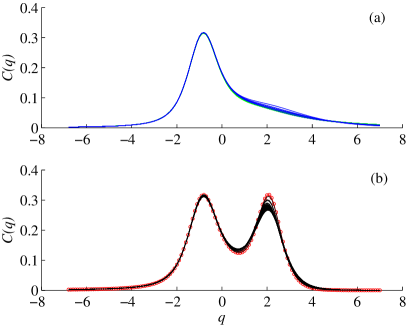
presents special effects when the string of economic data includes that of a crash. We shall refer to this quantity as analogous specific heat (ASpH). Using the S&P500 data corresponding to the 1987 market crash known as Black Monday (BM), it has been shown in Ref. [26] that these curves present two lobes when the time series of $N$ elements contains the data point of the crash. Further, the maxima of ASpH, $C(q)$, diminishes when the single data point from the day of the crash is removed and it disappears when the data of the neighboring days is deleted [26]. This lobe is due to the presence of large fluctuations ($q>0$) in the portion of the time series calculated. In Fig. 1 we show accumulated curves for $C(q)$ for Dow Jones data for windows of time before and after the crash, in particular Fig. 1(a) represents the accumulated curves for 50 days before the crash and Fig. 1(b), for 50 days after -and including- the crash. The dotted curve corresponds to BM day. Further in the text we will complete the description of these curves.

Figure 1: Accumulated analogous Specific heat, $C(q)$, for the crisis of 1987, Dow Jones index, (a) $50$ beginning with Black Monday (19 October 1987), (b) $50$ days after Black Monday. Dots correspond to $BM$. Here $N=1000$, $T=1$ and $l=1$.

To study the differences in the ASpH along the complete time series of size $L$, let us consider a window of size $N$ as a section of the series to be analyzed. This window is shifted along the data, with a given shift $l$, less or equal to $N$. $T$, $N$ and $l$ are parameters to be chosen for the particular system under consideration and the values are not predetermined. They are chosen as the best set for a given type of data, their selection will depend on the stability of results which will be discussed below. We calculate the area under the curve of ASpH, which we call $A(n)$, where $n$ is the index that identifies the window where our calculation is done, that is the number of shifts that we had performed. To identify the corresponding index in the complete series we notice that

$$t^{\prime}_{n}=t_{0}+N+n\,l,$$ (5)

where $t_{0}$ is the time where the calculation starts, and $n=1$ corresponds to $t^{\prime}_{1}=t_{0}+N$ of the series considered. Since the areas are calculated over a long period of time they possess a long memory, which is not necessarily desirable when we are near a crash or in a succession of them. In order to obtain seemingly uniform information we define the area variation rate (AVR) $\zeta(n)$ as

$$\zeta(n)=\left|\frac{A(n)}{\bar{A}}-1\right|,$$ (6)

where the mean $\bar{A}$ is calculated over all the windows previous to $n$. When there is no particular event in a time series this parameter fluctuates around or below $10^{-3}$ - see inset in Fig. 2. Although we do not have any proof, this seems to be always the case and it agrees with the AVR generated by white noise as will be seen below.

Figure 2: Plot of the area variation rate $\zeta(n)$ for the daily index for different events: Crash of ’29, $n_{s}=30$ corresponds to 24 October 1929 (red triangles) and $n_{O}=-20$; crisis of ’87, $n_{s}=40$ refers to 19 October 1987 (green squares), $n_{O}=-10$; crisis of $2008$, $n_{s}=50$ represents the bankrupcy of Lehman Brothers (cyan diamonds) and $n_{O}=0$; events of 2011, we show the AVR of the Dow Jones data where $n_{s}=70$ corresponds to 5 August 2011 (lilac empty circles) and $n_{O}=20$ and that of the FTSE100 series, which is non noticeable in this graph (blue filled circles), $n_{O}=30$. For this case we have used $T=1$, $l=1$ and $N=1000$.

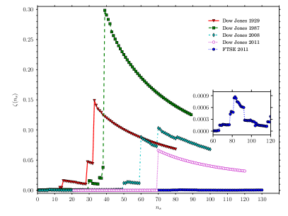
To apply this method we use daily closing indexes from different markets: Dow Jones, DAX, FTSE100, CAC, S&P 500 and Nasdaq, although not all results are shown. The data was obtained from finance.yahoo.com. The complete URL’s and the dates of downloading the data are given in reference [34]. The AVR for financial market daily data over a period of $100$ days is drawn in Fig. 2 for several well known events: the crisis of 1929, 1987, 2008 and 2011. All plots start $50$ days before the event that history identifies as the day of the corresponding crash, as done for Fig. 1. Thus, all the data used for the calculation of the AVR of a given day is prior to the date. In order to be able to notice their common features as well as their differences all the curves are plotted in the same graph with shifted origins$(n_{O})$. The crash of ’29 is shown in red triangles, where $n_{s}=n+n_{O}=30$ corresponds to 24 October 1929, known as Black Thursday (BT). The curve in green squares plots the same data, $n_{s}=40$ marks 19 October 1987, or Black Monday (BM). Next, in cyan diamonds, we present the same parameter AVR for the financial crisis of the year 2008, which was called the Subprime Crisis, and compared by the Press to the crash of ’29. Although there is a jump in the curve, it is well below the other curves. The value of $n_{s}=50$ corresponds to 15 September 2008, when Lehman Brothers announced bankruptcy, event which may have produced the succesive jumps at $n_{s}=60$ and $n_{s}=70$. Next, in lilac empty circles is the area variation rate for the Dow Jones 2011 data, where $n_{s}=70$ corresponds to 5 August. This date was chosen since on that day Standard and Poor’s announced the decrease in the credit ratings of the United States [35]. Therefore it is only natural to expect some reaction of the market. This is the only event worth mentioning in the Dow Jones data during 2011. Finally, in blue filled circles we show FTSE100 during 2011, which stays below $10^{-3}$ throughout the year (partially shown in the inset of Fig. 2). Apart from Dow Jones and FTSE100, we analyzed other European markets for 2011: DAX (Germany) and CAC (France). All of them, except the FTSE100, have some fluctuation above average in the summer of 2011 and a noticeable jump around 6 December 2011 - day when the results of a discussion on the survival of the Euro was announced. All fluctuations are within the same order of magnitude but below 1.5%.

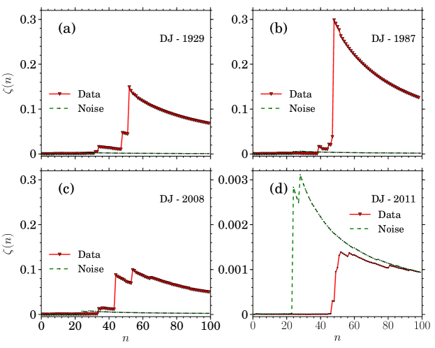
From that figure we notice that the AVR rises above noise at least one week before the crash for 1929, 1987 and 2008, characteristic that may be used as an indicator of the coming event. There is no significant fluctuation in the AVR during 2011. To distinguish if the increase is related to the crash we compare these results with the AVR index of a randomly generated time series (noise). The data used to calculate the AVR of the noise was obtained from a long series generated from white noise (independent and normally distributed), with the same mean and variance of the corresponding Dow Jones index. A value that “rises above noise” is at least one order of magnitude larger than these fluctuations. Results for the four cases discussed previously can be seen in Fig 3. It is interesting to notice that noise and 2011 fluctuations are of the same order of magnitude.

Figure 3: Plot of the area variation rate $\zeta(n)$ for the Dow Jones daily index and for randomly generated time series with the same average and variance of the corresponding Dow Jones index with parameter values $l=1$, $T=1$, $N=1000$ for: a) Crash of 1929; b) Crash of 1987; c) Subprime crisis 2008; d) Data centered around 5 August 2011

Figure 4: (a) Analogous specific heat, $C(q)$, for Dow Jones data corresponding to the Subprime crisis, 2008. (b) Plot of the corresponding area variation rate, $\zeta(n)$. (c) $C(q)$ for Dow Jones 2011. (d) Plot of the area variation rate, $\zeta(n)$, for 2011, the jump corresponds to 5 August 2011.All curves were calculated with $l=1$, $T=1$, $N=1000$

To interpret the importance of the AVR in the identification of crises, we recall that in Figs. 1(a) and 1(b) we show the accumulated curves for the ASpH individually calculated over each window of length $N$ previous to the point $n$. When we move to $n+1$, we slide the window onwards a quantity $l$ (shift) and calculate $C(q)$ again. There are $50$ overlapping curves in each figure and they are both types: single and doubled lobes. There is a clear change of shape in the curve corresponding to BM, already identified by Canessa by exclusion of the crash day’s data in his calculation. The distinct shape that the curve has on the 19th October shows the sensitivity of the method to the inclusion of the data of the crash since it is only one point within $N$ that produces a dramatic change in the figures. But the most important feature in the identification of the crisis is that the second peak of the curve $C(q)$, for $q>0$, appears at the same moment when the curve AVR jumps, and it does only if the jump is large, thus clearly pointing at the crash, which is produced by the very large fluctuations. Therefore large fluctuations in the market data give rise to the second maximum in the ASpH, which originate a discontinuity in the AVR, while robustness in $N$, $T$ and $l$ help to identify a crisis.

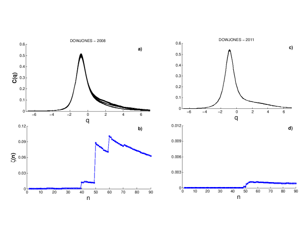
Next, we analyze the accumulated curves $C(q)$ for all the cases shown in Fig. 2, we have found a clear second lobe for the crises of ’29 and ’87. In particular let us focus our attention in the accumulated ASpH calculated along $n$ for 2008 and 2011 (Fig.  4(a) and Fig. 4(c), respectively) and the corresponding area variation rate as a function of $n$ - Fig. 4(b) and Fig. 4(d), respectively. There is no well defined second maximum in ASpH for 2008, although the results are robust against changes in $N$ and $T$ (not shown). For 2011 we detect no significant jumps in the AVR, no changes in the ASpH and the results do not persist under changes in the parameters (shown next).

Figure 5: Area variation rate, $\zeta(n)$, as a function of $n$, for different values of $T$: (a) Dow Jones crash October 1929; (b) Dow Jones crash October 1987; (c) Dow Jones Subprime crisis of 2008; (d) Dow Jones August 2011. All curves were calculated with $l=1$ and $N=1000$

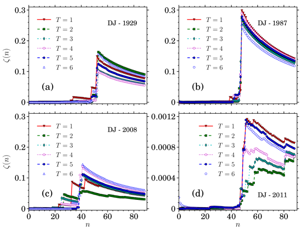
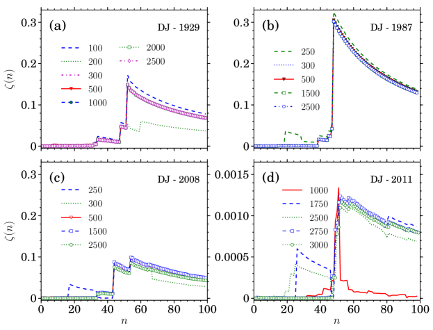
A small size window may produce false positives. Investigating the Dow Jones data over a century, it is noted that sometimes the AVR presents unexpected jumps. However, most of those jumps do not exhibit the pattern observed in the famous crashes and the jumps tend to vanish increasing the window size $N$ and $T$. In Fig. 5 results are shown for the AVR of all cases when varying the time lag. Results for 1929, 1987 and 2008 remain stable. For 2011, the jump on 5 August changes shape while staying always below or around noise level. We show similar results but varying N in Fig. 6, starting at a very low window size, $N=100$ for 1929. The AVR for 1929, 1987 and 2008 rapidly converges to a final value. That for 2011 oscillates without ever reaching a stable value. Another important factor is that the features previous to the crash discussed before appear for all values of $N$ and $T$ with $T=1$ giving the best results. Most features disappear when the shift $l$ becomes of the order of $N$, which is expected. From these it appears as if the crisis of 2011 is of a different nature from the other three. Calculations for different parameters $N$ and $T$ will show a real crisis, real being defined as stable against variations of $N$, $T$ and $l$ by comparison with the events historically recognized as crises.

Figure 6: Area variation rate, $\zeta(n)$, as a function of $n$, for different values of $N$: (a) Dow Jones crash of 1929; (b) Dow Jones of 1987; (c) Dow Jones 2008; (d) Dow Jones August 2011. All curves calculated with $l=1$ and $T=1$

3 Summary

Summarizing, we have presented a method by which market crisis can be identified and distinguished from simple scares which could avoid diffusion of panic. We noticed that when a crisis is systemic it behaves as in the cases well recognized historically as crises. It is usually accompanied by a sizable increase in the area variation rate by several orders of magnitude. It corresponds to a crash only if the analogous specific heat also presents a second maximum. Finally, all results are stable under changes in $N$, $l$ and $T$. We notice that for some well known crisis such as the crash of ’29 and ’87, the AVR already shows a substantial increase above noise almost two weeks before the event creating expectations as to the possibility of being used as a warning signal. While it is quite clear that the existence of large fluctuations ($q>0$) produces stable jumps in AVR, the predictive ability of the algorithm seems to depend on the values of $T$. An important factor of this method is that all calculations are done using data preceding the singular event, thus making it extremely useful, in particular for medical cases such as epilepsy. Its identification through a electroencephalogram, performed by the recognition of a specific characteristic of the temporal series, is only done after the episode. A method based on the calculation of the AVR may help in predicting seizures. Although this is not a tool which can help to avoid crises, due to the simplicity of its use, it can be implemented to monitor economic or physiological data under the possibility of a crisis. More research is underway to study applications – in particular the possibility of foreseeing epileptic seizures – and to establish the algorithm in a sound mathematical basis.

References

- [1] B. B. Mandelbrot, The variation of certain speculative prices, J. Bus. 36, (1963) 394.
- [2] J. Giles, B. Mandelbrot, Father of fractals, Nature 432, (2004) 266.
- [3] C. J. G. Evertsz, Fractal Geometry of Financial Time Series, Fractals 3, (1995) 609.
- [4] R. N. Mantegna, H. E. Stanley, Scaling behaviour in the dynamics of an economic index, Nature 376, (1995) 46.
- [5] A. F. Crepaldi, C. Rodrigues Neto, F. F. Ferreira, G. Francisco, Multifractal Regime transition in a modified minority game model. Chaos, Solutions & Fractals, 42, Issue 3,(2009) 1364.
- [6] D. Grech, Z. Mazur, Can one make any crash prediction in finance using the local Hurst exponent idea?, Physica A 336, (2004) 133.
- [7] D. Grech, G. Pamula, The local Hurst exponent of the financial time series in the vicinity of crashes on the Polish stock exchange market, Physica A 387 (2008) 4299.
- [8] L. Czarnecki, D. Grech, G. Pamula, Comparison study of global and local approaches describing critical phenomena on the Polish stock exchange market, Physica A 387 (2008) 6801.
- [9] T. Preis, J. J. Schneider, H. E. Stanley, Switching processes in financial markets, PNAS 108, (2011) 7677.
- [10] T. Preis, H.S. Moat, H. E. Stanley, S.R. Bishop, Quantifying the Advantage of Looking Forward, Sci. Rep. 2, (2012) 350; DOI:10.1038/srep00350 (2012).
- [11] D. Y. Kenett, Y. Shapira, A. Madi, S. Bransburg-Zabary, G. Gur-Gershgoren, E. Ben-Jacob, Index Cohesive Force Analysis Reveals That the US Market Became Prone to Systemic Collapses Since 2002, PLoS ONE 6(4): e19378.
- [12] D. Y. Kenett, M. Raddant, T. Lux, E. Ben-Jacob, Evolvement of Uniformity and Volatility in the Stressed Global Financial Village, PLoS ONE 7(2): e31144.
- [13] O. Pont, A. Turiel, C.J. Perez-Vicente, Empirical evidences of a common multifractal signature in economic, biological and physical systems, Physica A 388, (2009) 2025. 473.
- [14] X. Sun, H. Chen, Y. Yuan, Z. Wu, Predictability of multifractal analysis of Hang Seng stock index in Hong Kong, Physica A 301, (2001) 473.
- [15] K. Domino, The use of the Hurst exponent to predict changes in trends on the Warsaw Stock Exchange, Physica A 390, (2011) 98.
- [16] A. Johansen, O. Ledoit, D. Sornette, Crashes as Critical Points, Int. J. Theor. Applied Finance 3, (2000) 219.
- [17] D. Sornette, Wei-Xing Zhou, Predictability of large future changes in major financial indices, Int. J. Forecast. 22, (2006) 153.
- [18] D. Sornette, R. Woodard, Wei-Xing Zhou, The 2006-2008 oil bubble: Evidence of speculation, and prediction, Physica A388, (2009) 1571.
- [19] D. Harmon, M. de Aguiar, D. Chinellato, D. Braha, I. Epstein, Y. Bar-Yam, Predicting economic market crises using measures of collective panic, 2011, arXiv:1102.2620.
- [20] Y. Shapira, D. Y. Kenett, Ohad Raviv, and E. Ben-Jacob, Hidden temporal order unveiled in stock market volatility variance, AIP ADVANCES 1, (2011) 022127.
- [21] V. Misra, M. Lagi, Y. Bar-Yam, Evidence of market manipulation in the financial crisis, 2011, arXiv:1112.3095
- [22] P. Ball, The new history, Nature 480, (2011) 447.
- [23] O. A. Rosso, C. Masoller, Detecting and quantifying stochastic and coherence resonances via information-theory complexity measurements, Phys. Rev. E 79, (2009) 040106(R).
- [24] O. A. Rosso, C. Masoller, Detecting and quantifying temporal correlations in stochastic resonance via information theory measures, Eur. Phys. J. B 69, (2009) 37.
- [25] J. F. Donges, R. V. Donner, Martin H. Trauth, N. Marwan, H.-J. Schellnhuber, J. Kurths, Nonlinear detection of paleoclimate-variability transitions possibly related to human evolution, PNAS 108, (2011) 20422.
- [26] E. Canessa, Langevin dynamics of financial systems: A second-order analysis, Eur. Phys. J. B 22, (2001) 123.
- [27] J. Lee, H. E. Stanley, Phase Transition in the Multifractal spectrum of Diffusion-Limited Aggregation, Phys. Rev. Lett. 61, (1988) 2945.
- [28] S. Kumar, N. Deo, Multifractal properties of the Indian financial market, Physica A 388, (2009) 1593.
- [29] J. Barunik, T. Aste, T. Di Matteo, R. Liu, Understanding the Source of Multifractality in Financial Markets, Physica A 391, (2012) 4234.
- [30] A. Rényi, On measures of information and entropy, Proceedings of the 4th Berkeley Symposium on Mathematics, Statistics and Probability 1960, (1961) 547.
- [31] F. O. Redelico, A. N. Proto, An empirical fractal geometry analysis of some financial speculative bubbles, Physica A 391, (2012) 5132.
- [32] K. Ivanova, H. N. Shirer, E. E. Clothiaux, N. Kitova, M. A. Mikhalev, T. P. Ackerman, M. Ausloos, A case study of stratus cloud base height multifractal fluctuations, Physica A 308, (2002) 518.
- [33] K. Ivanova, M. Ausloos, Low q-moment Multifractal Analysis of Gold price, Dow Jones Industrial Average and BGL-USD exchange rate, Eur. Phys. J. B 8, (1999) 665.
-
[34]
Sources of financial market data:
http://uk.finance.yahoo.com/q/hp?s=^FTSE (downloaded 6 January 2012);
http://fr.finance.yahoo.com/q/hp?s=^GDAXI (downloaded 6 January 2012);
http://fr.finance.yahoo.com/q/hp?s=^FCHI (downloaded 7 January 2012) -
[35]
http://www.standardandpoors.com/ratings/articles/en/us/?assetID=1245316529563
;
http://www.reuters.com/article/2011/08/08/us-usa-rating-sandp-clearinghouses-idUSTRE7774I620110808