Exact expressions for the intercepts of $r$-particle momentum correlation functions in $\mu$-Bose gas model

A.M. Gavrilik and Yu.A. Mishchenko
Abstract

Recently, the deformed $\mu$-Bose gas model based on so called $\mu$-deformed oscillators was proposed. For that model, the intercepts of $r$-particle momentum correlation functions (correlation functions at coinciding momenta of particles) were treated for $r=2,3$, within certain order of approximation in $\mu$. In this work, we derive for $\mu$-Bose gas model the exact expressions for $r$-particle correlation function intercepts, for all $r$, through Lerch transcendent and find their asymptotics (as functions of $\mu$). For 2-, 3-particle intercepts and deformed distribution function ⟨ak†​ak⟩delimited-⟨⟩subscriptsuperscriptš‘Žā€ š‘˜subscriptš‘Žš‘˜\langle a^{\dagger}_{k}a_{k}\rangle the dependence on particles momentum is presented graphically.

Keywords: deformed Bose gas model, deformed oscillators, non-standard statistics, intercepts of correlation functions, Lerch transcendent.
PACS: 05.30.Jp; 05.90.+m; 11.10.Lm; 25.75.Gz; 02.30.Gp.

1 Introduction

The deformed $\mu$-Bose gas modelĀ [1] is a particular implementation of such an efficient in nonlinear quantum physics tools as deformed oscillators (for their definition, diverse models and some applications, see e.g.Ā [2]). The latter provide a generalization of the quantum harmonic oscillator and are often used in effective descriptions of various nontrivial properties of nonlinear systems and/or phenomena. Due to an effective representation in terms of deformed oscillator(s) we may come to a more simple system whose behavior approximates the behavior of the initial one. Main properties of a deformed oscillator and its distinction from the standard quantum harmonic oscillator are characterized by the corresponding deformation structure function $\phi(N)$ (seeĀ [3, 2, 4] for its notion). Depending on $\phi(N)$ one distinguishes many types of deformed oscillators. Say, the one used in the elaboration of $\mu$-Bose gas model is called $\mu$-oscillator and was introduced inĀ [5]. Besides this rather exotic $\mu$-deformed oscillator (for which, $\phi(N)=\frac{N}{1+\mu N}$) there are such well-known $q$-deformed oscillators as Arik-CoonĀ [6] and Biedenharn-MacfarlaneĀ [7, 8] ones, the $p,q$-deformed oscillator defined inĀ [9] and also the $q$-deformed Tamm-Dancoff oscillatorĀ [10, 11]. Let us note that the latter four deformed oscillator models belong to the class of Fibonacci oscillatorsĀ [12] (i.e. such that their structure function $\phi_{n}\equiv\phi(n)$ satisfies Fibonacci-like three-term recurrence relation with constant coefficients). Unlike, the $\mu$-oscillator represents the class of so-called quasi-Fibonacci deformed oscillators treated inĀ [13] and that implies some peculiarities in concrete applications.

Besides the $\mu$-Bose gas model there exist many other deformed Bose gas models in which deformed oscillators were utilized. To list a few, the $q$-Bose gas model was studied inĀ [14] (see also the references therein), $p,q$-Bose gas model was investigated inĀ [15, 16] and in some other works. Thermodynamical aspects of deformed Bose gases were studied e.g. inĀ [17, 18, 19]. It is worth to mention that deformed oscillators were also effectively used for modelling a gas of (nonpointlike, composite) particles or quasiparticlesĀ [20, 21, 22], in the study of Bose-Einstein condensationĀ [23] and of phonon spectrum in ${}^{4}He$Ā [24], for the description of interacting particles systemsĀ [25]. As it was shown inĀ [26, 27], it is possible to realize composite bosons in terms of deformed oscillators (deformed bosons), and to relate the inter-component entanglement just with the parameter of deformationĀ [28]. In the context of $n$-particle correlations, deformed oscillators were applied inĀ [14, 15, 16], and the corresponding intercepts of correlation functions (along with their asymptotics) were obtained as functions of deformation parameter.

In the preceding paperĀ [1] the approximate expressions to certain order in $\mu$ were obtained for the intercepts of the 2nd and 3rd order momentum correlation functions in the deformed $\mu$-Bose gas model, and for the corresponding asymptotics the exact expressions were found. It turns out that the results for the $r$th order intercepts can be obtained in exact form and this constitutes main subject of the present work. In fact, we derive the corresponding exact formulae given in terms of Lerch Phi-function (Lerch transcendent) for the general case of $r$-particle correlation intercept and also illustrate some of them graphically, with special attention to the particular cases $r=2$ and $r=3$. One can hope that present results and further development $\mu$-Bose gas model, say, concerning thermodynamical aspects will find effective applications to diverse physical systems.

2 Derivation of the exact expressions for intercepts of the correlation functions in $\mu$-Bose gas model

Our treatment concerns deformed $\mu$-Bose gas model as the secondary quantized system of specially deformed bosons. That means that each modeĀ š¤š¤\bf k in the deformed Bose gas is described by the deformed oscillator with the creation/annihilation operators aš¤ā€ subscriptsuperscriptš‘Žā€ š¤a^{\dagger}_{\bf k}, $a_{\bf k}$, and the number operator $N_{\bf k}$. The defining relations for such a system of deformed oscillators (deformed bosons) are given as

aš¤ā€ ā€‹aš¤=ϕ​(Nš¤),subscriptsuperscriptš‘Žā€ š¤subscriptš‘Žš¤italic-Ļ•subscriptš‘š¤\displaystyle a^{\dagger}_{\bf k}a_{\bf k}=\phi(N_{\bf k}), (1)
[aš¤,aš¤ā€²ā€ ]=Ī“š¤š¤ā€²ā€‹(ϕ​(Nš¤+1)āˆ’Ļ•ā€‹(Nš¤)),[aš¤,aš¤ā€²]=0,formulae-sequencesubscriptš‘Žš¤subscriptsuperscriptš‘Žā€ superscriptš¤ā€²subscriptš›æsuperscriptš¤š¤ā€²italic-Ļ•subscriptš‘š¤1italic-Ļ•subscriptš‘š¤subscriptš‘Žš¤subscriptš‘Žsuperscriptš¤ā€²0\displaystyle[a_{\bf k},a^{\dagger}_{\bf k^{\prime}}]=\delta_{\bf kk^{\prime}}\bigl{(}\phi(N_{\bf k}+1)-\phi(N_{\bf k})\bigr{)},\quad[a_{\bf k},a_{\bf k^{\prime}}]=0, (2)
[Nš¤,aš¤ā€²ā€ ]=Ī“š¤š¤ā€²ā€‹aš¤ā€ ,[Nš¤,aš¤ā€²]=āˆ’Ī“š¤š¤ā€²ā€‹aš¤,formulae-sequencesubscriptš‘š¤subscriptsuperscriptš‘Žā€ superscriptš¤ā€²subscriptš›æsuperscriptš¤š¤ā€²subscriptsuperscriptš‘Žā€ š¤subscriptš‘š¤subscriptš‘Žsuperscriptš¤ā€²subscriptš›æsuperscriptš¤š¤ā€²subscriptš‘Žš¤\displaystyle[N_{\bf k},a^{\dagger}_{\bf k^{\prime}}]=\delta_{\bf kk^{\prime}}a^{\dagger}_{\bf k},\quad[N_{\bf k},a_{\bf k^{\prime}}]=-\delta_{\bf kk^{\prime}}a_{\bf k}, (3)

where the concept of structure function $\phi(N)$ is used. As seen, we deal with the system of deformed oscillators which are mode independent i.e. the operators corresponding to deformed oscillators in different modes commute.

Like inĀ [1], and similarly to the corresponding nondeformed analogsĀ [29], the concerned intercepts of the $r$th order momentum correlation function at a given momentumĀ š¤š¤\bf k are defined as

Ī»(r)​(š¤)=⟨(aš¤ā€ )r​(aš¤)r⟩⟨aš¤ā€ ā€‹aš¤āŸ©rāˆ’1.superscriptšœ†š‘Ÿš¤delimited-⟨⟩superscriptsubscriptsuperscriptš‘Žā€ š¤š‘Ÿsuperscriptsubscriptš‘Žš¤š‘Ÿsuperscriptdelimited-⟨⟩subscriptsuperscriptš‘Žā€ š¤subscriptš‘Žš¤š‘Ÿ1\lambda^{(r)}({\bf k})=\frac{\langle(a^{\dagger}_{\bf k})^{r}(a_{\bf k})^{r}\rangle}{\langle a^{\dagger}_{\bf k}a_{\bf k}\rangle^{r}}-1. (4)

Symbol $\langle...\rangle$ denotes usual statistical average for a system with HamiltonianĀ Hš»H:

$$\langle F\rangle=\frac{\mathop{\mathrm{Tr}}\nolimits F\exp(-\beta H)}{\mathop{\mathrm{Tr}}\nolimits\exp(-\beta H)},$$ (5)

where $\beta=(k_{B}T)^{-1}$, $k_{B}$ is Boltzmann constant. Using (1) and (3) the formulaĀ (4) for the interceptsĀ Ī»(r)​(š¤)superscriptšœ†š‘Ÿš¤\lambda^{(r)}({\bf k}) can be rewritten in terms of the structure function $\phi(N)$ as

$$\lambda^{(r)}({\bf k})=\frac{\langle[N_{\bf k}][N_{\bf k}-1]\cdot...\cdot[N_{\bf k}-r+1]\rangle}{\langle[N_{\bf k}]\rangle^{r}}-1,$$ (6)

where the notation $[N]=[N]_{\phi}\equiv\phi(N)$ for the structure function is used. Since we deal with the $\mu$-deformed Bose gas modelĀ [1], for $\phi(N)$ we take the structure function of $\mu$-deformed oscillator:

$$\phi_{\mu}(N)\equiv[N]_{\mu}=\frac{N}{1+\mu N},\quad\mu>0.$$

The interceptsĀ (6) depend on the choice of Hamiltonian $H$. We choose the Hamiltonian in the form

$$H=\sum_{\bf k}\hbar\omega_{\bf k}N_{\bf k}$$ (7)

and assume that deformed boson energy depends only on the absolute value $k=|{\bf k}|$ of the momentum. Then, using the Fock-like basis in which $N_{\bf k}|n_{\bf k}\rangle=n_{\bf k}|n_{\bf k}\rangle$, $\phi(N_{\bf k})|n_{\bf k}\rangle=\phi(n_{\bf k})|n_{\bf k}\rangle$, the mode independence, and taking into account (5)-(7), for the $r$-particle correlation function intercept we obtain

$$\lambda^{(r)}_{\mu}(k)=\frac{(1-e^{-\beta\hbar\omega})^{-r+1}\sum_{n=0}^{\infty}\frac{n}{1+\mu n}\cdot...\cdot\frac{n-r+1}{1+\mu(n-r+1)}\exp\bigl{[}-\beta\hbar\omega n\bigr{]}}{\Bigl{(}\sum_{n=0}^{\infty}\frac{n}{1+\mu n}\exp\bigl{[}-\beta\hbar\omega n)\bigr{]}\Bigr{)}^{r}}-1,\ \ \omega\!=\!\omega_{\bf k}\!=\!\omega(k).$$ (8)

As seen, the intercept depends on $\mu$, on the momentum absolute value $k$ and temperature $T$. To proceed, we expand the product in the $n$th summand of the numerator series (in front of exponent) into the sum of simple fractions:

$$\prod_{l=0}^{r-1}\frac{n-l}{1+\mu(n-l)}=\frac{1}{\mu^{r}}\prod_{l=0}^{r-1}\Bigl{(}1-\frac{1}{1+\mu(n\!-\!l)}\Bigr{)}=\frac{1}{\mu^{r}}+\frac{1}{\mu^{r}}\sum_{l=0}^{r-1}\frac{A^{(r)}_{l}(\mu)}{1+\mu(n-l)}.$$ (9)

The coefficientsĀ Al(r)​(μ)subscriptsuperscriptš“š‘Ÿš‘™šœ‡A^{(r)}_{l}(\mu) obey the recurrence relations:

$$\left\{\begin{aligned} &A^{(r+1)}_{l}(\mu)=A^{(r)}_{l}(\mu)\Bigl{(}1+\frac{1}{\mu(r-l)}\Bigr{)},\quad l=0,...,r-1;\\ &A^{(r+1)}_{r}(\mu)=-1-\sum_{l=0}^{r-1}\frac{A^{(r)}_{l}(\mu)}{\mu(r-l)}.\end{aligned}\right.$$ (10)

These relations allow to find the coefficients $A^{(r)}_{l}$, to list a few:

$\displaystyle A^{(1)}_{0}(\mu)=-1;$
$\displaystyle A^{(2)}_{0}(\mu)=-1-\frac{1}{\mu},\quad A^{(2)}_{1}(\mu)=-1+\frac{1}{\mu};$
$\displaystyle A^{(3)}_{0}(\mu)=-1-\frac{3}{2\mu}-\frac{1}{2\mu^{2}},\quad A^{(3)}_{1}(\mu)=-1+\frac{1}{\mu^{2}},\quad A^{(3)}_{2}(\mu)=-1+\frac{3}{2\mu}-\frac{1}{2\mu^{2}};$
$\displaystyle\ldots\,.$

Then, in view ofĀ (9)-(10) the infinite sum in the numerator ofĀ (8) can be rewritten as

$$\sum_{n=0}^{\infty}\frac{n}{1+\mu n}\cdot...\cdot\frac{n-r+1}{1+\mu(n-r+1)}\exp\bigl{[}-\beta\hbar\omega n\bigr{]}=\frac{1}{\mu^{r}}\sum_{n=0}^{\infty}\exp\bigl{[}-\beta\hbar\omega n\bigr{]}+\\ +\frac{1}{\mu^{r}}\sum_{l=0}^{r-1}A^{(r)}_{l}(\mu)\sum_{n=0}^{\infty}\frac{1}{1+\mu(n-l)}\exp\bigl{[}-\beta\hbar\omega n\bigr{]}.$$ (11)

Likewise for the sum in the denominator ofĀ (8) we obtain

$$\sum_{n=0}^{\infty}\frac{n}{1+\mu n}\exp\bigl{[}-\beta\hbar\omega n\bigr{]}=\frac{1}{\mu}\sum_{n=0}^{\infty}\exp\bigl{[}-\beta\hbar\omega n\bigr{]}+\frac{1}{\mu}A^{(1)}_{0}(\mu)\sum_{n=0}^{\infty}\frac{1}{1+\mu n}\exp\bigl{[}-\beta\hbar\omega n\bigr{]}.$$ (12)

As seen, the second series in the r.h.s. ofĀ (11) andĀ (12) are of similar form. Therefore in order to calculate this expression it is enough to perform summation of the generic series, that yields:

$\displaystyle\sum_{n=0}^{\infty}\frac{1}{a+bn}e^{-\beta\hbar\omega n}=\sum_{n=0}^{\infty}\frac{z^{n}}{a+bn}\equiv\frac{1}{b}\Phi(z,1,a/b)=\frac{1}{b}\Phi(e^{-\beta\hbar\omega},1,a/b),$
$\displaystyle a=1-\mu l,\ \ b=\mu,\ \ l=1,...,r-1,\quad\ \ z=e^{-\beta\hbar\omega},$

where $\Phi$ is the Lerch transcendent, see e.g. [30].

As result we arrive at the following expression for the thermal average ⟨ak†​ak⟩delimited-⟨⟩subscriptsuperscriptš‘Žā€ š‘˜subscriptš‘Žš‘˜\langle a^{\dagger}_{k}a_{k}\rangle

$$\langle a^{\dagger}_{k}a_{k}\rangle=\langle\phi(N_{k})\rangle=\left\{\begin{aligned} &(e^{\beta\hbar\omega}-1)^{-1},\quad\mu=0,\\ &\mu^{-1}-\mu^{-2}(1-e^{-\beta\hbar\omega})\Phi(e^{-\beta\hbar\omega},1,\mu^{-1}),\quad\mu>0,\end{aligned}\right.$$ (13)

and the $r$th order averages (deformed analogs of $r$-particle momentum distribution)

⟨(ak†)r​(ak)r⟩=1+Ī¼āˆ’1​(1āˆ’eāˆ’Ī²ā€‹ā„ā€‹Ļ‰)ā€‹āˆ‘l=0rāˆ’1Al(r)​(μ)​Φ​(eāˆ’Ī²ā€‹ā„ā€‹Ļ‰,1,Ī¼āˆ’1āˆ’l),r≄2,formulae-sequencedelimited-⟨⟩superscriptsubscriptsuperscriptš‘Žā€ š‘˜š‘Ÿsuperscriptsubscriptš‘Žš‘˜š‘Ÿ1superscriptšœ‡11superscriptš‘’š›½Planck-constant-over-2-pišœ”superscriptsubscriptš‘™0š‘Ÿ1subscriptsuperscriptš“š‘Ÿš‘™šœ‡Ī¦superscriptš‘’š›½Planck-constant-over-2-pišœ”1superscriptšœ‡1š‘™š‘Ÿ2\langle(a^{\dagger}_{k})^{r}(a_{k})^{r}\rangle=1+\mu^{-1}(1-e^{-\beta\hbar\omega})\sum_{l=0}^{r-1}A^{(r)}_{l}(\mu)\Phi(e^{-\beta\hbar\omega},1,\mu^{-1}-l),\quad r\geq 2, (14)

which constitute one of our main results. The limit $\mu\rightarrow 0$ applied toĀ (14) has a peculiarity, so we calculate ⟨(ak†)r​(ak)r⟩delimited-⟨⟩superscriptsubscriptsuperscriptš‘Žā€ š‘˜š‘Ÿsuperscriptsubscriptš‘Žš‘˜š‘Ÿ\langle(a^{\dagger}_{k})^{r}(a_{k})^{r}\rangle for $\mu=0$ separately. Starting from its definition we arrive at

⟨(ak†)r​(ak)r⟩|μ=0=(1āˆ’eāˆ’Ī²ā€‹ā„ā€‹Ļ‰)ā€‹āˆ‘n=0āˆžn​(nāˆ’1)​…​(nāˆ’r+1)​eāˆ’Ī²ā€‹ā„ā€‹Ļ‰ā€‹n.evaluated-atdelimited-⟨⟩superscriptsubscriptsuperscriptš‘Žā€ š‘˜š‘Ÿsuperscriptsubscriptš‘Žš‘˜š‘Ÿšœ‡01superscriptš‘’š›½Planck-constant-over-2-pišœ”superscriptsubscriptš‘›0š‘›š‘›1ā€¦š‘›š‘Ÿ1superscriptš‘’š›½Planck-constant-over-2-pišœ”š‘›\langle(a^{\dagger}_{k})^{r}(a_{k})^{r}\rangle|_{\mu=0}=(1-e^{-\beta\hbar\omega})\sum_{n=0}^{\infty}n(n-1)...(n-r+1)e^{-\beta\hbar\omega n}.

Using Abel’s identity for the latter sum we obtain:

(1āˆ’eāˆ’Ī²ā€‹ā„ā€‹Ļ‰)āˆ‘n=0āˆžn(nāˆ’1)…(nāˆ’r+1)eāˆ’Ī²ā€‹ā„ā€‹Ļ‰ā€‹n=(1āˆ’eāˆ’Ī²ā€‹ā„ā€‹Ļ‰)limNā†’āˆž{N(Nāˆ’1)…(Nāˆ’r+1)eāˆ’Ī²ā€‹ā„ā€‹Ļ‰ā€‹(N+1)āˆ’1eāˆ’Ī²ā€‹ā„ā€‹Ļ‰āˆ’1āˆ’āˆ’āˆ‘n=0Nāˆ’1rn(nāˆ’1)…(nāˆ’r+2)eāˆ’Ī²ā€‹ā„ā€‹Ļ‰ā€‹(n+1)āˆ’1eāˆ’Ī²ā€‹ā„ā€‹Ļ‰āˆ’1}=(1āˆ’eāˆ’Ī²ā€‹ā„ā€‹Ļ‰)reĪ²ā€‹ā„ā€‹Ļ‰āˆ’1āˆ‘n=0āˆžn(nāˆ’1)…(nāˆ’r+2)eāˆ’Ī²ā€‹ā„ā€‹Ļ‰ā€‹n==reĪ²ā€‹ā„ā€‹Ļ‰āˆ’1ā€‹āŸØ(ak†)rāˆ’1​(ak)rāˆ’1⟩|μ=0=…=r!(eĪ²ā€‹ā„ā€‹Ļ‰āˆ’1)r1superscriptš‘’š›½Planck-constant-over-2-pišœ”superscriptsubscriptš‘›0š‘›š‘›1ā€¦š‘›š‘Ÿ1superscriptš‘’š›½Planck-constant-over-2-pišœ”š‘›1superscriptš‘’š›½Planck-constant-over-2-pišœ”subscriptā†’š‘š‘š‘1ā€¦š‘š‘Ÿ1superscriptš‘’š›½Planck-constant-over-2-pišœ”š‘11superscriptš‘’š›½Planck-constant-over-2-pišœ”1superscriptsubscriptš‘›0š‘1š‘Ÿš‘›š‘›1ā€¦š‘›š‘Ÿ2superscriptš‘’š›½Planck-constant-over-2-pišœ”š‘›11superscriptš‘’š›½Planck-constant-over-2-pišœ”11superscriptš‘’š›½Planck-constant-over-2-pišœ”š‘Ÿsuperscriptš‘’š›½Planck-constant-over-2-pišœ”1superscriptsubscriptš‘›0š‘›š‘›1ā€¦š‘›š‘Ÿ2superscriptš‘’š›½Planck-constant-over-2-pišœ”š‘›evaluated-atš‘Ÿsuperscriptš‘’š›½Planck-constant-over-2-pišœ”1delimited-⟨⟩superscriptsubscriptsuperscriptš‘Žā€ š‘˜š‘Ÿ1superscriptsubscriptš‘Žš‘˜š‘Ÿ1šœ‡0ā€¦š‘Ÿsuperscriptsuperscriptš‘’š›½Planck-constant-over-2-pišœ”1š‘Ÿ(1-e^{-\beta\hbar\omega})\sum_{n=0}^{\infty}n(n-1)...(n-r+1)e^{-\beta\hbar\omega n}=(1-e^{-\beta\hbar\omega})\lim_{N\rightarrow\infty}\biggl{\{}N(N-1)...(N-r+1)\frac{e^{-\beta\hbar\omega(N+1)}-1}{e^{-\beta\hbar\omega}-1}-\\ -\sum_{n=0}^{N-1}r\,n(n-1)...(n-r+2)\frac{e^{-\beta\hbar\omega(n+1)}-1}{e^{-\beta\hbar\omega}-1}\biggr{\}}=(1-e^{-\beta\hbar\omega})\frac{r}{e^{\beta\hbar\omega}-1}\sum_{n=0}^{\infty}n(n-1)...(n-r+2)e^{-\beta\hbar\omega n}=\\ =\frac{r}{e^{\beta\hbar\omega}-1}\langle(a^{\dagger}_{k})^{r-1}(a_{k})^{r-1}\rangle|_{\mu=0}=\ldots=\frac{r!}{(e^{\beta\hbar\omega}-1)^{r}}

Thus,

⟨(ak†)r​(ak)r⟩|μ=0=r!(eĪ²ā€‹ā„ā€‹Ļ‰āˆ’1)r.evaluated-atdelimited-⟨⟩superscriptsubscriptsuperscriptš‘Žā€ š‘˜š‘Ÿsuperscriptsubscriptš‘Žš‘˜š‘Ÿšœ‡0š‘Ÿsuperscriptsuperscriptš‘’š›½Planck-constant-over-2-pišœ”1š‘Ÿ\langle(a^{\dagger}_{k})^{r}(a_{k})^{r}\rangle|_{\mu=0}=\frac{r!}{(e^{\beta\hbar\omega}-1)^{r}}. (15)

From (13)-(14) and eq.(4) we obtain our next result – the intercept $\lambda^{(r)}_{\mu}(k)$ of $r$th order correlation function,

$\displaystyle\lambda^{(r)}_{\mu}(k)=\Bigl{(}1+\mu^{-1}(1-e^{-\beta\hbar\omega})\sum_{l=0}^{r-1}A^{(r)}_{l}(\mu)\Phi(e^{-\beta\hbar\omega},1,\mu^{-1}-l)\Bigr{)}\cdot$
$\displaystyle\cdot\Bigl{(}1+\mu^{-1}(1-e^{-\beta\hbar\omega})A^{(1)}_{0}(\mu)\Phi(e^{-\beta\hbar\omega},1,\mu^{-1})\Bigr{)}^{-r}-1,\quad r=2,3,...\,,\quad\text{if}\ \mu>0,$ (16)

Using (15), in the no-deformation limit $\mu\rightarrow 0$ we recover:

$$\lambda^{(r)}_{\mu}(k)|_{\mu=0}=r!-1.$$ (17)

The obtained formula (2) presents the exact general expression for the intercepts under consideration as it covers all the orders $r\geq 2$.

3 Series expansions in $\mu$

In the case of small deformation parameter $\mu$ it may be of interest to have an expansion of $\lambda^{(r)}_{\mu}(k)$ in $\mu$. For that goal we expand the generic series present in (11) and (12) as follows:

āˆ‘n=0āˆž11+μ​(nāˆ’l)​eāˆ’Ī±ā€‹n=āˆ‘s=0āˆžcs​(l)​μs,α=Ī²ā€‹ā„ā€‹Ļ‰,l=0,…,rāˆ’1.formulae-sequencesuperscriptsubscriptš‘›011šœ‡š‘›š‘™superscriptš‘’š›¼š‘›superscriptsubscriptš‘ 0subscriptš‘š‘ š‘™superscriptšœ‡š‘ formulae-sequenceš›¼š›½Planck-constant-over-2-pišœ”š‘™0ā€¦š‘Ÿ1\sum_{n=0}^{\infty}\frac{1}{1+\mu(n-l)}e^{-\alpha n}=\sum_{s=0}^{\infty}c_{s}(l)\mu^{s},\quad\alpha=\beta\hbar\omega,\ l=0,...,r-1. (18)

The coefficients cs​(l)subscriptš‘š‘ š‘™c_{s}(l) of the expansion are found as

$$c_{s}(l)=\frac{1}{s!}\frac{\partial{{}^{s}}}{\partial{\mu^{s}}}\sum_{n=0}^{\infty}\frac{1}{1+\mu(n-l)}e^{-\alpha n}\Bigr{|}_{\mu=0}=e^{-\alpha l}\sum_{n=0}^{\infty}(-1)^{s}(n-l)^{s}e^{-\alpha(n-l)}=(-1)^{s}e^{-\alpha l}\sum_{n=-l}^{\infty}n^{s}e^{-\alpha n}=\\ =(-1)^{s}e^{-\alpha l}\Bigl{(}-\frac{\partial{}}{\partial{\alpha}}\Bigr{)}^{s}\sum_{n=-l}^{\infty}e^{-\alpha n}=e^{-\alpha l}\Bigl{(}\frac{\partial{}}{\partial{\alpha}}\Bigr{)}^{s}\frac{e^{\alpha l}}{1-e^{-\alpha}}=\frac{1}{x^{l}}\Bigl{(}x\frac{d}{dx}\Bigr{)}^{s}\frac{x^{l+1}}{x-1},\quad x=e^{\alpha}.$$

For the derivative in the last expression we perform the following transformation ($m=l+1$):

(x​dd​x)s​xmxāˆ’1superscriptš‘„š‘‘š‘‘š‘„š‘ superscriptš‘„š‘šš‘„1\displaystyle\Bigl{(}x\frac{d}{dx}\Bigr{)}^{s}\frac{x^{m}}{x-1} =(x​dd​x)s​xmāˆ’1xāˆ’1+(x​dd​x)s​1xāˆ’1=(x​dd​x)sā€‹āˆ‘j=0māˆ’1xj+(x​dd​x)s​1xāˆ’1=absentsuperscriptš‘„š‘‘š‘‘š‘„š‘ superscriptš‘„š‘š1š‘„1superscriptš‘„š‘‘š‘‘š‘„š‘ 1š‘„1superscriptš‘„š‘‘š‘‘š‘„š‘ superscriptsubscriptš‘—0š‘š1superscriptš‘„š‘—superscriptš‘„š‘‘š‘‘š‘„š‘ 1š‘„1absent\displaystyle=\Bigl{(}x\frac{d}{dx}\Bigr{)}^{s}\frac{x^{m}-1}{x-1}+\Bigl{(}x\frac{d}{dx}\Bigr{)}^{s}\frac{1}{x-1}=\Bigl{(}x\frac{d}{dx}\Bigr{)}^{s}\sum_{j=0}^{m-1}x^{j}+\Bigl{(}x\frac{d}{dx}\Bigr{)}^{s}\frac{1}{x-1}=
=Ī“s​0+āˆ‘j=1māˆ’1js​xj+(x​dd​x)s​1xāˆ’1.absentsubscriptš›æš‘ 0superscriptsubscriptš‘—1š‘š1superscriptš‘—š‘ superscriptš‘„š‘—superscriptš‘„š‘‘š‘‘š‘„š‘ 1š‘„1\displaystyle=\delta_{s0}+\sum_{j=1}^{m-1}j^{s}x^{j}+\Bigl{(}x\frac{d}{dx}\Bigr{)}^{s}\frac{1}{x-1}.

By induction it can be checked that the latter derivative may be presented as the finite sum:

(x​dd​x)s​1xāˆ’1=āˆ‘j=0s(āˆ’1)sj+1​gsj(xāˆ’1)j+1superscriptš‘„š‘‘š‘‘š‘„š‘ 1š‘„1superscriptsubscriptš‘—0š‘ superscript1š‘ š‘—1superscriptsubscriptš‘”š‘ š‘—superscriptš‘„1š‘—1\Bigl{(}x\frac{d}{dx}\Bigr{)}^{s}\frac{1}{x-1}=\sum_{j=0}^{s}\frac{(-1)^{s}}{j+1}\frac{g_{s}^{j}}{(x-1)^{j+1}}

where the coefficients gsjsuperscriptsubscriptš‘”š‘ š‘—g_{s}^{j} satisfy the recurrence relation

gs+1j=(j+1)​(gsj+gsjāˆ’1),g00=1.formulae-sequencesubscriptsuperscriptš‘”š‘—š‘ 1š‘—1superscriptsubscriptš‘”š‘ š‘—superscriptsubscriptš‘”š‘ š‘—1superscriptsubscriptš‘”001g^{j}_{s+1}=(j\!+\!1)(g_{s}^{j}+g_{s}^{j-1}),\quad g_{0}^{0}=1.

The solution of this recurrence relation is expressed through the Stirling numbers of the second kind {sj}FRACOPš‘ š‘—\bigl{\{}{s\atop j}\bigr{\}}:

gsj=(j+1)!​{s+1j+1}.superscriptsubscriptš‘”š‘ š‘—š‘—1FRACOPš‘ 1š‘—1g_{s}^{j}=(j+1)!\Bigl{\{}{s\!+\!1\atop j\!+\!1}\Bigr{\}}.

In view of the latter, the coefficients cs​(l)subscriptš‘š‘ š‘™c_{s}(l) take the form

cs​(l)=Ī“s​0​eāˆ’Ī²ā€‹ā„ā€‹Ļ‰ā€‹l+eāˆ’Ī²ā€‹ā„ā€‹Ļ‰ā€‹lā€‹āˆ‘j=1ljs​eĪ²ā€‹ā„ā€‹Ļ‰ā€‹j+eāˆ’Ī²ā€‹ā„ā€‹Ļ‰ā€‹l​(āˆ’1)sā€‹āˆ‘j=0sj!​{s+1j+1}​1(eĪ²ā€‹ā„ā€‹Ļ‰āˆ’1)j+1.subscriptš‘š‘ š‘™subscriptš›æš‘ 0superscriptš‘’š›½Planck-constant-over-2-pišœ”š‘™superscriptš‘’š›½Planck-constant-over-2-pišœ”š‘™superscriptsubscriptš‘—1š‘™superscriptš‘—š‘ superscriptš‘’š›½Planck-constant-over-2-pišœ”š‘—superscriptš‘’š›½Planck-constant-over-2-pišœ”š‘™superscript1š‘ superscriptsubscriptš‘—0š‘ š‘—FRACOPš‘ 1š‘—11superscriptsuperscriptš‘’š›½Planck-constant-over-2-pišœ”1š‘—1c_{s}(l)=\delta_{s0}e^{-\beta\hbar\omega l}+e^{-\beta\hbar\omega l}\sum_{j=1}^{l}j^{s}e^{\beta\hbar\omega j}+e^{-\beta\hbar\omega l}(-1)^{s}\sum_{j=0}^{s}j!\Bigl{\{}{s\!+\!1\atop j\!+\!1}\Bigr{\}}\frac{1}{(e^{\beta\hbar\omega}-1)^{j+1}}.

Let us write out several first coefficients:

$\displaystyle c_{0}(0)=1+\frac{1}{(e^{\beta\hbar\omega}\!-\!1)},$
$\displaystyle c_{1}(0)=-\frac{1}{(e^{\beta\hbar\omega}\!-\!1)}-\frac{1}{(e^{\beta\hbar\omega}\!-\!1)^{2}},$
$\displaystyle c_{2}(0)=\frac{1}{(e^{\beta\hbar\omega}\!-\!1)}+\frac{3}{(e^{\beta\hbar\omega}\!-\!1)^{2}}+\frac{2}{(e^{\beta\hbar\omega}\!-\!1)^{3}},$
$\displaystyle c_{3}(0)=-\frac{1}{(e^{\beta\hbar\omega}\!-\!1)}-\frac{7}{(e^{\beta\hbar\omega}\!-\!1)^{2}}-\frac{12}{(e^{\beta\hbar\omega}\!-\!1)^{3}}-\frac{6}{(e^{\beta\hbar\omega}\!-\!1)^{4}},$
$\displaystyle c_{4}(0)=\frac{1}{(e^{\beta\hbar\omega}\!-\!1)}+\frac{15}{(e^{\beta\hbar\omega}\!-\!1)^{2}}+\frac{50}{(e^{\beta\hbar\omega}\!-\!1)^{3}}+\frac{60}{(e^{\beta\hbar\omega}\!-\!1)^{4}}+\frac{24}{(e^{\beta\hbar\omega}\!-\!1)^{5}},$
$\displaystyle c_{5}(0)=-\frac{1}{(e^{\beta\hbar\omega}\!-\!1)}-\frac{31}{(e^{\beta\hbar\omega}\!-\!1)^{2}}-\frac{180}{(e^{\beta\hbar\omega}\!-\!1)^{3}}-\frac{390}{(e^{\beta\hbar\omega}\!-\!1)^{4}}-\frac{360}{(e^{\beta\hbar\omega}\!-\!1)^{5}}-\frac{120}{(e^{\beta\hbar\omega}\!-\!1)^{6}},$
$\displaystyle c_{6}(0)=\frac{1}{(e^{\beta\hbar\omega}\!-\!1)}+\frac{63}{(e^{\beta\hbar\omega}\!-\!1)^{2}}+\frac{602}{(e^{\beta\hbar\omega}\!-\!1)^{3}}+\frac{2100}{(e^{\beta\hbar\omega}\!-\!1)^{4}}+\frac{3360}{(e^{\beta\hbar\omega}\!-\!1)^{5}}+\frac{2520}{(e^{\beta\hbar\omega}\!-\!1)^{6}}+\frac{840}{(e^{\beta\hbar\omega}\!-\!1)^{7}}.$

Using the ā€œinitialā€ coefficients cs​(0)subscriptš‘š‘ 0c_{s}(0), all other coefficients can be determined by the formula

cs​(l)=eāˆ’Ī²ā€‹ā„ā€‹Ļ‰ā€‹lā€‹āˆ‘j=1ljs​eĪ²ā€‹ā„ā€‹Ļ‰ā€‹j+eāˆ’Ī²ā€‹ā„ā€‹Ļ‰ā€‹l​cs​(0).subscriptš‘š‘ š‘™superscriptš‘’š›½Planck-constant-over-2-pišœ”š‘™superscriptsubscriptš‘—1š‘™superscriptš‘—š‘ superscriptš‘’š›½Planck-constant-over-2-pišœ”š‘—superscriptš‘’š›½Planck-constant-over-2-pišœ”š‘™subscriptš‘š‘ 0c_{s}(l)=e^{-\beta\hbar\omega l}\sum_{j=1}^{l}j^{s}e^{\beta\hbar\omega j}+e^{-\beta\hbar\omega l}c_{s}(0).

Then the sumsĀ (11) andĀ (12), the latter being a particular case of the former, have the following Taylor expansions:

āˆ‘n=0āˆžn1+μ​n⋅…⋅nāˆ’r+11+μ​(nāˆ’r+1)​eāˆ’Ī²ā€‹ā„ā€‹Ļ‰ā€‹n=1μr​(1āˆ’eāˆ’Ī²ā€‹ā„ā€‹Ļ‰)āˆ’1+1μrā€‹āˆ‘s=0āˆžāˆ‘l=0rāˆ’1Al(r)​(μ)​cs​(l)​μs,superscriptsubscriptš‘›0ā‹…š‘›1šœ‡š‘›ā€¦š‘›š‘Ÿ11šœ‡š‘›š‘Ÿ1superscriptš‘’š›½Planck-constant-over-2-pišœ”š‘›1superscriptšœ‡š‘Ÿsuperscript1superscriptš‘’š›½Planck-constant-over-2-pišœ”11superscriptšœ‡š‘Ÿsuperscriptsubscriptš‘ 0superscriptsubscriptš‘™0š‘Ÿ1subscriptsuperscriptš“š‘Ÿš‘™šœ‡subscriptš‘š‘ š‘™superscriptšœ‡š‘ \displaystyle\sum_{n=0}^{\infty}\frac{n}{1\!+\!\mu n}\cdot...\cdot\frac{n\!-\!r\!+\!1}{1\!+\!\mu(n\!-\!r\!+\!1)}e^{-\beta\hbar\omega n}=\frac{1}{\mu^{r}}(1-e^{-\beta\hbar\omega})^{-1}+\frac{1}{\mu^{r}}\sum_{s=0}^{\infty}\sum_{l=0}^{r-1}A^{(r)}_{l}(\mu)c_{s}(l)\,\mu^{s}, (19)
āˆ‘n=0āˆžn1+μ​n​eāˆ’Ī²ā€‹ā„ā€‹Ļ‰ā€‹n=1μ​(1āˆ’eāˆ’Ī²ā€‹ā„ā€‹Ļ‰)āˆ’1+1Ī¼ā€‹āˆ‘s=0āˆžA0(1)​(μ)​cs​(0)​μs.superscriptsubscriptš‘›0š‘›1šœ‡š‘›superscriptš‘’š›½Planck-constant-over-2-pišœ”š‘›1šœ‡superscript1superscriptš‘’š›½Planck-constant-over-2-pišœ”11šœ‡superscriptsubscriptš‘ 0subscriptsuperscriptš“10šœ‡subscriptš‘š‘ 0superscriptšœ‡š‘ \displaystyle\sum_{n=0}^{\infty}\frac{n}{1\!+\!\mu n}e^{-\beta\hbar\omega n}=\frac{1}{\mu}(1-e^{-\beta\hbar\omega})^{-1}+\frac{1}{\mu}\sum_{s=0}^{\infty}A^{(1)}_{0}(\mu)c_{s}(0)\,\mu^{s}. (20)

The series (19) and (20) can be shown to be divergent for any $\mu>0$ and, so, their practical use is doubtful.

4 Particular cases and comparison with results from other deformed Bose-gas models

Consider two particular cases $r=2$ and $r=3$, earlier considered inĀ [1] within a prescribed approximation. In these two cases, for the intercepts $\lambda^{(2)}_{\mu}$ and $\lambda^{(3)}_{\mu}$ ($0<\mu<\frac{1}{2}$) we obtain:

$\displaystyle\lambda^{(2)}_{\mu}=(1-e^{-\beta\hbar\omega})^{-1}\Bigl{\{}(1-e^{-\beta\hbar\omega})^{-1}-\Bigl{(}\frac{1}{\mu}+\frac{1}{\mu^{2}}\Bigr{)}\Phi(e^{-\beta\hbar\omega},1,\mu^{-1})-\Bigl{(}\frac{1}{\mu}-\frac{1}{\mu^{2}}\Bigr{)}\Phi(e^{-\beta\hbar\omega},1,\mu^{-1}\!-\!1)\Bigr{\}}\cdot$
$\displaystyle\qquad\Bigl{(}(1-e^{-\beta\hbar\omega})^{-1}-\mu^{-1}\Phi(e^{-\beta\hbar\omega},1,\mu^{-1})\Bigr{)}^{-2}-1,$ (21)
$\displaystyle\lambda^{(3)}_{\mu}=(1\!-\!e^{-\beta\hbar\omega})^{-2}\Bigl{\{}(1\!-\!e^{-\beta\hbar\omega})^{-1}\!-\!\Bigl{(}\frac{1}{\mu}\!+\!\frac{3}{2\mu^{2}}\!+\!\frac{1}{2\mu^{3}}\Bigr{)}\Phi(e^{-\beta\hbar\omega},1,\mu^{-1})\!-\!\Bigl{(}\frac{1}{\mu}\!-\!\frac{1}{\mu^{3}}\Bigr{)}\Phi(e^{-\beta\hbar\omega},1,\mu^{-1}\!-\!1)-$
$\displaystyle\qquad-\Bigl{(}\frac{1}{\mu}\!-\!\frac{3}{2\mu^{2}}\!+\!\frac{1}{2\mu^{3}}\Bigr{)}\Phi(e^{-\beta\hbar\omega},1,\mu^{-1}\!-\!2)\Bigr{\}}\cdot\Bigl{(}(1\!-\!e^{-\beta\hbar\omega})^{-1}-\mu^{-1}\Phi(e^{-\beta\hbar\omega},1,\mu^{-1})\Bigr{)}^{-3}-1.$ (22)

It is worth also to consider the following specially constructedĀ [31] functionĀ rμ(3)​(k)subscriptsuperscriptš‘Ÿ3šœ‡š‘˜r^{(3)}_{\mu}(k) (also considered inĀ [16, 1]), useful in the experimental context:

$$r^{(3)}_{\mu}(k)=\frac{\lambda^{(3)}_{\mu}(k)-3\lambda^{(2)}_{\mu}(k)}{2(\lambda^{(2)}_{\mu}(k))^{3/2}}.$$ (23)

It implies cancellation of unwanted distortions and provides improved purity. With account ofĀ (23) and the exact expressions (21)-(22) the explicit result for $r^{(3)}_{\mu}(k)$ readily follows merely by substitution (so we don’t reproduce it here).

In case when deformed bosons (here of $\mu$-Bose gas) are used like inĀ [14, 16, 1] to describe relativistic particles, the energy is specified as $\hbar\omega_{k}=\sqrt{m^{2}+k^{2}}$. Then, the dependence of ⟨ak†​ak⟩delimited-⟨⟩subscriptsuperscriptš‘Žā€ š‘˜subscriptš‘Žš‘˜\langle a^{\dagger}_{k}a_{k}\rangle, $\lambda^{(2)}_{\mu}(k,T)$, $\lambda^{(3)}_{\mu}(k,T)$ and $r^{(3)}_{\mu}(k,T)$ on the momentumĀ k=|š¤|š‘˜š¤k=|{\bf k}| for the values $\mu=0.1,\,0.2$ of deformation parameter, the temperatures being $T=120,\,180\,MeV$, is such as shown in Figures 2, 2, 4 and 4.
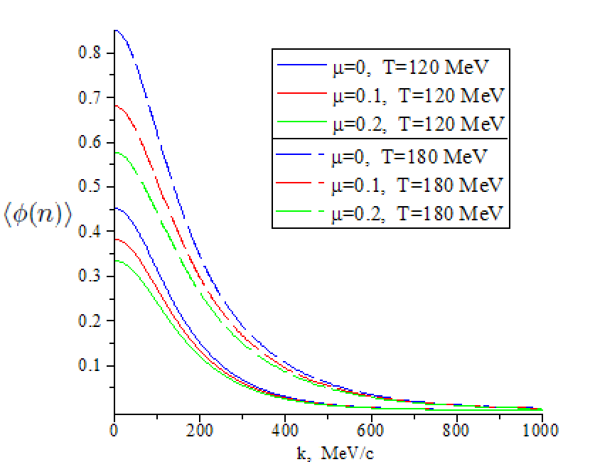
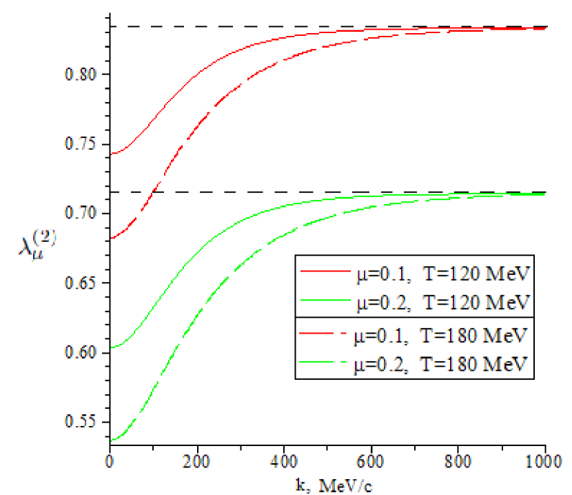
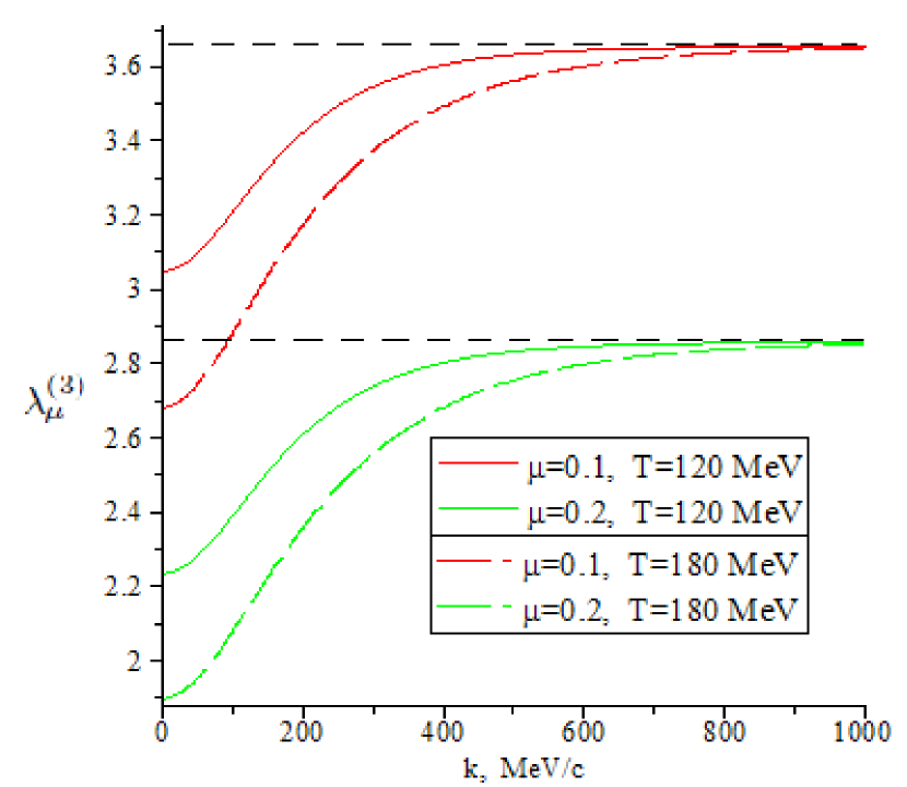
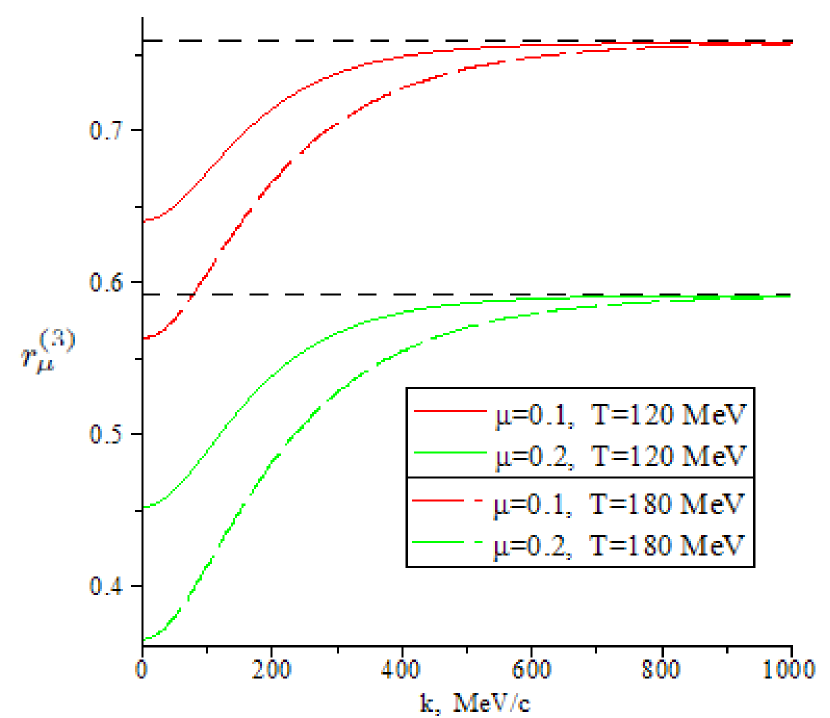
Refer to caption
Figure 1: Dependence of the deformed distribution āŸØĻ•ā€‹(N)⟩=⟨ak†​ak⟩delimited-⟨⟩italic-Ļ•š‘delimited-⟨⟩subscriptsuperscriptš‘Žā€ š‘˜subscriptš‘Žš‘˜\langle\phi(N)\rangle=\langle a^{\dagger}_{k}a_{k}\rangle on the momentum $k$, for deformation parameter values $\mu=0$ (pure Bose case) and $\mu=0.1,\,0.2$ (deformed case) and temperatures $T=120,\,180\,MeV$
Refer to caption
Figure 2: Dependence of the intercept $\lambda^{(2)}_{\mu}(k)$ on the momentum $k$, for deformation parameter values $\mu=0.1,\,0.2$ and temperatures $T=120,\,180\,MeV$. Asymptotes are found fromĀ (27) at $\mu=0.1,\,0.2$.
Refer to caption
Figure 3: Dependence of the intercept $\lambda^{(3)}_{\mu}(k)$ on the momentum $k$, for deformation parameter values $\mu=0.1,\,0.2$ and temperatures $T=120,\,180\,MeV$. Asymptotes are found fromĀ (27) at $\mu=0.1,\,0.2$.
Refer to caption
Figure 4: Dependence of the correlation function $r^{(3)}_{\mu}(k)$ fromĀ (23) on the momentum $k$, for deformation parameter values $\mu=0.1,\,0.2$ and temperatures $T=120,\,180\,MeV$. Asymptotes stem fromĀ (23) after the substitution ofĀ (27).

From fig.Ā 2 we see that the curves of deformed distributions lie below the usual ($\mu=0$) nondeformed Bose-Einstein one; with the increase of deformation parameterĀ Ī¼šœ‡\mu or decrease of temperature $T$ the curves go lower and lower. For the momentum dependence of the intercepts $\lambda^{(2)}_{\mu}(k)$, $\lambda^{(3)}_{\mu}(k)$, and the functionĀ rμ(3)​(k)subscriptsuperscriptš‘Ÿ3šœ‡š‘˜r^{(3)}_{\mu}(k) (figuresĀ 2-4) we observe the similar behavior with respect toĀ Ī¼šœ‡\mu – larger deformation parametersĀ Ī¼šœ‡\mu correspond to lower curves, while lower temperatures correspond to curves lying higher. Besides, for all the plots in figuresĀ 2-4 the dependence on the momentumĀ kš‘˜k shows asymptotical tending to the corresponding constant values for the intercepts (given byĀ (27) below), with the large momentum asymptotics forĀ rμ(3)​(k)subscriptsuperscriptš‘Ÿ3šœ‡š‘˜r^{(3)}_{\mu}(k) stemming fromĀ (23).

The remaining part of this section is devoted to a comparison of the results obtained above with the analogous results presented in earlier papers on other deformed Bose gas models. The comparison concerns the correlation intercepts along with their asymptotics found within $\mu$-Bose gas modelĀ [1], and those found in deformed Bose gas model of another type. For instance, in the case of $p,q$-Bose gas model the exact expression for the deformed analog of $r$-particle distribution and for the intercept of the $r$th order correlation function obtained inĀ [15] respectively read (denote $[r]_{p,q}!\equiv[r]_{p,q}[r-1]_{p,q}...[1]_{p,q}$):

⟨(Ak†)r​(Ak)r⟩=[r]p​q!​(eā„ā€‹Ī²ā€‹Ļ‰āˆ’1)āˆj=0r(eā„ā€‹Ī²ā€‹Ļ‰āˆ’pj​qrāˆ’j),delimited-⟨⟩superscriptsubscriptsuperscriptš“ā€ š‘˜š‘Ÿsuperscriptsubscriptš“š‘˜š‘Ÿsubscriptdelimited-[]š‘Ÿš‘š‘žsuperscriptš‘’Planck-constant-over-2-piš›½šœ”1superscriptsubscriptproductš‘—0š‘Ÿsuperscriptš‘’Planck-constant-over-2-piš›½šœ”superscriptš‘š‘—superscriptš‘žš‘Ÿš‘—\displaystyle\langle(A^{\dagger}_{k})^{r}(A_{k})^{r}\rangle=\frac{[r]_{pq}!(e^{\hbar\beta\omega}-1)}{\prod_{j=0}^{r}(e^{\hbar\beta\omega-p^{j}q^{r-j}})}, (24)
Ī»p,q(r)​(k)=⟨(Ak†)r​(Ak)r⟩⟨Ak†​Ak⟩rāˆ’1=[r]p,q!​(eā„ā€‹Ļ‰āˆ’p)r​(eā„ā€‹Ļ‰āˆ’q)r(eā„ā€‹Ļ‰āˆ’1)rāˆ’1ā€‹āˆj=0r(eā„ā€‹Ļ‰āˆ’qrāˆ’j​pj)āˆ’1.subscriptsuperscriptšœ†š‘Ÿš‘š‘žš‘˜delimited-⟨⟩superscriptsubscriptsuperscriptš“ā€ š‘˜š‘Ÿsuperscriptsubscriptš“š‘˜š‘Ÿsuperscriptdelimited-⟨⟩subscriptsuperscriptš“ā€ š‘˜subscriptš“š‘˜š‘Ÿ1subscriptdelimited-[]š‘Ÿš‘š‘žsuperscriptsuperscriptš‘’Planck-constant-over-2-pišœ”š‘š‘Ÿsuperscriptsuperscriptš‘’Planck-constant-over-2-pišœ”š‘žš‘Ÿsuperscriptsuperscriptš‘’Planck-constant-over-2-pišœ”1š‘Ÿ1superscriptsubscriptproductš‘—0š‘Ÿsuperscriptš‘’Planck-constant-over-2-pišœ”superscriptš‘žš‘Ÿš‘—superscriptš‘š‘—1\displaystyle\lambda^{(r)}_{p,q}(k)=\frac{\langle(A^{\dagger}_{k})^{r}(A_{k})^{r}\rangle}{\langle A^{\dagger}_{k}A_{k}\rangle^{r}}-1=[r]_{p,q}!\frac{(e^{\hbar\omega}-p)^{r}(e^{\hbar\omega}-q)^{r}}{(e^{\hbar\omega}-1)^{r-1}\prod\nolimits_{j=0}^{r}(e^{\hbar\omega}-q^{r-j}p^{j})}-1. (25)

With respect to the corresponding resultĀ (2) of the present paper, the expressionĀ (25), even though involving two parameters of deformation, has a simpler form (expressed in terms of elementary functions, not special ones), and this is presumably connected with the fact that $p,q$-oscillator belongs to the Fibonacci class whereas $\mu$-oscillator represents the class of quasi-FibonacciĀ [13] oscillators (therefore its treatment is more involved).

Now let us examine the asymptotic behavior. It is seen that the correlation intercepts tend to certain constant values at large momenta. These asymptotical values of $\lambda^{(r)}_{\mu}(k,T)$ depend on $\mu$ only, and can be obtained directly from the definitionĀ (8) by taking the limit

λμ,a​s​y​m​p​t(r)=subscriptsuperscriptšœ†š‘Ÿšœ‡š‘Žš‘ š‘¦š‘šš‘š‘”absent\displaystyle\lambda^{(r)}_{\mu,\,asympt}= $\displaystyle\lim_{\omega\to\infty}\frac{\sum_{n=0}^{\infty}\frac{n}{1+\mu n}\cdot...\cdot\frac{n-r+1}{1+\mu(n-r+1)}e^{-\beta\hbar\omega n}}{(1-e^{-\beta\hbar\omega})^{r-1}\Bigl{(}\sum_{n=0}^{\infty}\frac{n}{1+\mu n}e^{-\beta\hbar\omega n}\Bigr{)}^{r}}-1=\lim_{\omega\to\infty}\frac{[r]_{\mu}!e^{-\beta\hbar\omega r}+...}{\bigl{(}\frac{1}{1+\mu}\bigr{)}^{r}e^{-\beta\hbar\omega r}+...}-1=$
$\displaystyle=$ $\displaystyle\bigl{(}1+\mu\bigr{)}^{r}[r]_{\mu}!-1,\qquad\qquad[r]_{\mu}!\equiv[r]_{\mu}[r-1]_{\mu}...[1]_{\mu}.$ (26)

In the numerator, the dominating $n=r$ term is retained whereas in the denominator the $n=1$ term dominates. For $r=2$ and $r=3$ this result is in complete agreement with the corresponding asymptotical values of the $\mu$-Bose gas intercepts $\lambda^{(2)}$ and $\lambda^{(3)}$ earlier found inĀ [1]:

λμ,a​s​y​m​p​t(2)=(1+μ)2​[2]μ!āˆ’1=11+2​μ,λμ,a​s​y​m​p​t(3)=(1+μ)3​[3]μ!āˆ’1=5+7​μ(1+2​μ)​(1+3​μ).formulae-sequencesubscriptsuperscriptšœ†2šœ‡š‘Žš‘ š‘¦š‘šš‘š‘”superscript1šœ‡2subscriptdelimited-[]2šœ‡1112šœ‡subscriptsuperscriptšœ†3šœ‡š‘Žš‘ š‘¦š‘šš‘š‘”superscript1šœ‡3subscriptdelimited-[]3šœ‡157šœ‡12šœ‡13šœ‡\lambda^{(2)}_{\mu,\,asympt}=\bigl{(}1+\mu\bigr{)}^{2}[2]_{\mu}!-1=\frac{1}{1+2\mu},\qquad\lambda^{(3)}_{\mu,\,asympt}=\bigl{(}1+\mu\bigr{)}^{3}[3]_{\mu}!-1=\frac{5+7\mu}{(1+2\mu)(1+3\mu)}. (27)

It is instructive to compare the asymptotical valuesĀ (26) of the $r$th order correlation intercepts for $\mu$-Bose gas model with the corresponding asymptotics in the case of $p,q$-Bose gas modelĀ [15, 16], that is

Ī»p​q,a​s​y​m​p​t(r)=[r]p,q!āˆ’1.subscriptsuperscriptšœ†š‘Ÿš‘š‘žš‘Žš‘ š‘¦š‘šš‘š‘”subscriptdelimited-[]š‘Ÿš‘š‘ž1\lambda^{(r)}_{pq,\,asympt}=[r]_{p,q}!-1. (28)

The distinction, expressed on the $\mu$-Bose gas side by the extra factorĀ (1+μ)rsuperscript1šœ‡š‘Ÿ\bigl{(}1+\mu\bigr{)}^{r}, is connected with the fact that for $p,q$-oscillator we have $[1]_{p,q}=1$, whereas for $\mu$-oscillator $[1]_{\mu}=\frac{1}{1+\mu}\neq 1$. The exact expression for the asymptotics of the functionĀ rμ(3)​(k)subscriptsuperscriptš‘Ÿ3šœ‡š‘˜r^{(3)}_{\mu}(k) can be obtained like inĀ [1] by substitution ofĀ (27) into (23).

5 Concluding remarks

This work describes further steps with respect toĀ [1] – here we extend those results and find them in precise form. More specifically, within $\mu$-Bose gas model we have obtained the exact expressionsĀ (2), (17) for the intercepts of $r$th order correlation functions for any $r\geq 2$, as well as the explicit formulae (13)-(15) for (deformed and non-deformed) one- and $r$-particle distributions. Recall that inĀ [1] the corresponding formulae were given only for the cases $r=2$ and $r=3$, and within certain approximation. Here the exact expressions for these particular cases ($r=2$ and $r=3$) are presented inĀ (21) and (22) above. We have also obtained exact formula which gives the asymptotical values for the $r$th order correlation functions intercepts, as the corresponding functions ofĀ Ī¼šœ‡\mu. Taylor expansions in the deformation parameterĀ Ī¼šœ‡\mu for one- and $r$-particle (deformed) distributions are obtained, seeĀ (19) and (20). Further analysis shows that they turn out to be divergent for any $\mu>0$.

The dependence on the momentum $k$ of thermal average ⟨ak†​ak⟩delimited-⟨⟩subscriptsuperscriptš‘Žā€ š‘˜subscriptš‘Žš‘˜\langle a^{\dagger}_{k}a_{k}\rangle, of the second and third order intercepts $\lambda^{(2)}_{\mu}(k)$ and $\lambda^{(3)}_{\mu}(k)$, as well as of the function $r^{(3)}_{\mu}(k)$, seeĀ (23), was illustrated in the corresponding figuresĀ 2-4. The comparison of the obtained results with those of previous papers shows that the plots of $\lambda^{(2)}_{\mu}(k)$, $\lambda^{(3)}_{\mu}(k)$ and $r^{(3)}_{\mu}(k)$ are in qualitative agreement with earlier results. Moreover, the corresponding large momentum asymptotics of $\lambda^{(2)}_{\mu}(k)$ and $\lambda^{(3)}_{\mu}(k)$ completely agree with those found inĀ [1]. If we compare the asymptoticsĀ (26) with the analogous asymptoticsĀ (28) found, also for arbitrary order $r$, within the $p,q$-deformationĀ [15] we observe the following. In the both cases the corresponding deformation of $r$-factorial does appear, but the resultĀ (26) differs from the formulaĀ (28), see alsoĀ [15], by presence of the extra factor $(1+\mu)^{r}$ – this is caused by differing values of the deformation structure functions at $n=1$. At last, few words concerning the further research on the relevant issues. For more comprehensive treatment of the $\mu$-Bose gas model studied here and inĀ [1] it is desirable to calculate some thermodynamic quantities (e.g. the critical temperature of condensation, the equation of state in the form of virial expansion) for $\mu$-Bose gas, like this was done inĀ [32] for the $p,q$-Bose gas model.

Acknowledgements

The authors are thankful to A.P. Rebesh for useful discussions. This research was partially supported by the Special Program of the Division of Physics and Astronomy of the NAS of Ukraine.

References