Thermal transport of molecular junctions in the pair tunneling regime

Abstract

Charge and heat transport through a single molecule tunnel-coupled to external normal electrodes have been studied. The molecule with sufficiently strong interaction between electrons and vibrational internal degrees of freedom can be characterized by the negative effective charging energy U$<0$. Such a molecule has been considered and modeled by the Anderson Hamiltonian. The electrical conductance, thermopower and thermal conductance of the system have been calculated as a function of gate voltage in the weak coupling limit within the rate equation approach. In the linear regime the analytic formulae for the transport coefficients in the pair dominated tunneling are presented. The effects found in the nonlinear transport include inter alia the rectification of the heat current. The sense of forward (reverse) direction, however, depends on the tuning parameter and can be controlled by the gate voltage. We also discuss the quantitation of the thermal conductance and the departures from the Wiedemann-Franz law.

I Introduction

The appearance of the effective attractive interactions between electrons in metals BCS is responsible for the instability of the Fermi surface and the resulting phenomenon of superconductivity; one of the most spectacular quantum effects on a macroscopic scale. The strong local electron – phonon interaction may induce formation of polaron or bipolaron quasiparticles which are at the heart of bipolaronic theory of superconductivity micnas1990 ; alexandrov1994 . The so-called negative U centers anderson1975 are not only a source of superconducting instability but also play an important role in physics and chemistry of materials varma1988 (see, however harrison2006 ).

The tendency towards bipolaron formation is enhanced alexandrov1995 in the confined structures like quantum dotsjacak1998 . This assertion has been corroborated by means of quantum Monte Carlo calculations in the strong coupling regime for various dimensionalities of nano-structures hohenadler2007 . Negative charging energy of the small systems like quantum dots is a relatively new concept Koch ; alexandrov2002 ; holmqvist2008 ; gierczak2008 . Very small system is characterized by the small capacitance $C$ which makes the charging energy $e^{2}/2C$ large. To overcome it sufficiently strong polaronic shifts resulting from strong coupling of vibrational and charge degrees of freedom in a molecule are needed. The charge fluctuations in a device with metallic and superconducting grains may also over-screen the Kondo repulsion holmqvist2008 in the normal grain.

The purpose of this paper is to extend the recent work Koch in which charge transport through the molecule galperin2007 characterized by the negative charging energy has been studied. Modeling the system using Anderson like Hamiltonian with a negative value of the charging energy $U$ and considering weak coupling between the molecule and the electrodes the authors have systematically accounted for the processes contributing to charge transport and calculated its differential conductance. The study of the negative U molecule has later been extended to the stronger coupling and the regime of the charge Kondo effectkoch2007 .

Here we consider the same model and study the charge and heat transport via negative U molecule in the weak coupling regime when the pair tunneling processes dominate the transport. The analytical formulas for the thermopower $S$ and the thermal conductivity $\kappa$ in the linear regime of the low bias voltage $V=(\mu_{L}-\mu_{R})/e$ and the temperature difference $\delta T=T_{L}-T_{R}$ have been found. $\mu_{L(R)}$ denotes the chemical potential and $T_{L(R)}$ temperature of the left (right) external metallic bulk electrode. $e$ denotes the positive electron charge. As in the previous work we assume that the molecule is characterized by single, doubly degenerated electronic level. In the nonlinear regime with large temperature differences $\delta T$ and asymmetric coupling to the external leads the system shows heat rectification property. The thermal current and conductance in the forward direction (say, $\delta T>0$) differ from those in the reverse direction ($\delta T<0$).

The low temperature thermal conductance $\kappa$ in the linear regime is proportional to $T$, but the heat quantum, defined as $\kappa/T$ takes on a non-universal value. However, the Wiedemann-Franz law is obeyed in the limit $T\rightarrow 0$. At elevated temperatures we observe marked departures from the Fermi liquid behavior with the ratio $L=\kappa/(GT)$ exceeding the Lorenz number $L_{0}=\pi^{2}k_{B}^{2}/3e^{2}$.

The organization of the rest of the paper is as follows. In the next section we briefly recall the model and approach. In section III we present the transport coefficients calculated in the linear regime. In section IV the nonlinear transport coefficients are defined and calculated. In section V we discuss the validity of the Wiedemann-Franz law and quantization of the thermal conductance in the context of pair tunneling. We end up with summary and conclusions.

II The model and approach

The aim of this section is to recall the main results obtained by Koch et al. Koch and to establish the notation. One starts with a general system consisting of external leads and a central molecule coupled by tunneling processes. The electron subsystem on a molecule interacts with bosonic degrees of freedom (phonons), which are eliminated by performing the Firsov-Lang canonical transformation. We assume polaronic shifts large enough to make the effective charging energy $U_{eff}=U-2\lambda^{2}\hbar\omega$ negative. We denote it simply $U$. The motional narrowing of hopping parameters as well as shifts of the dot energy level are absorbed in the definition of the corresponding parameters in the Hamiltonian

$$H=H_{mol}+H_{leads}+H_{i}\,,$$ (1)

where $H_{mol}=\varepsilon_{d}n_{d}+Un_{d\uparrow}n_{d\downarrow}$ describes the interacting electrons on the dot. Here $n_{d}=\sum_{\sigma}n_{d\sigma}=\sum_{\sigma}d^{\dagger}_{\sigma}d_{\sigma}$ is the number operator, and $d^{\dagger}_{\sigma}(d_{\sigma})$ denotes the creation (annihilation) operator of a spin $\sigma$ electron on the molecule. The external leads (left-L and right-R) are characterized by the electron energy spectrum $\varepsilon_{\bf k}$. The corresponding term in the Hamiltonian is given by $H_{leads}=\sum_{\lambda=L,R}\sum_{{\bf k},\sigma}\xi_{\lambda,{\bf k}}c_{\lambda\,{\bf k}\,\sigma}^{\dagger}c_{\lambda\,{\bf k}\,\sigma}$, with $\xi_{\lambda\,{\bf k}}=\varepsilon_{\lambda\,{\bf k}}-\mu_{\lambda}$ and $\mu_{\lambda}=\mu-eV_{\lambda}$ denoting the chemical potential of the $\lambda$ electrode subject to the bias voltage $V_{\lambda}$. In the following we assume the equilibrium value of the chemical potential $\mu=0$ and $\epsilon_{L{\bf k}}=\epsilon_{R{\bf k}}=\epsilon_{{\bf k}}$.

The coupling between the molecule and leads is governed by the Hamiltonian

$$H_{i}=\sum_{\lambda=L,R}\sum_{{\bf k},\sigma}(t_{\lambda}c_{\lambda\,{\bf k}\,\sigma}^{\dagger}d_{\sigma}+h.c.)\,.$$ (2)

To correctly account for all low energy processes which contribute to the transport in the limit of negative $U$, it is advisable to eliminate $H_{i}$ by means of the Schrieffer-Wolff Schrieffer_Wolff transformation. This is valid in the limits $|t_{\lambda}|\ll|U+\varepsilon_{d}|$ and $|t_{\lambda}|\ll|\varepsilon_{d}|$ schuttler1988 . One gets Koch the effective low energy Hamiltonian

$$\tilde{H}=H_{mol}+H_{leads}+H_{dir,ex}+H_{pair},$$ (3)

in which the direct and exchange $H_{dir,ex}$ interactions between the dot and the leads read

$$H_{dir,ex}=\frac{1}{2}\sum_{\lambda\lambda^{\prime}{\bf k}{\bf k^{\prime}}\sigma}{t_{\lambda}t_{\lambda^{\prime}}^{*}}\bigg{[}\frac{1}{\varepsilon_{\lambda{\bf k}}-\varepsilon_{d}}c_{\lambda{\bf k}\sigma}^{\dagger}c_{\lambda^{\prime}{\bf k^{\prime}}\sigma}+$$ (4)

$$M(\varepsilon_{\lambda{\bf k}})(d_{-\sigma}^{\dagger}d_{\sigma}c_{\lambda{\bf k}\sigma}^{\dagger}c_{\lambda^{\prime}{\bf k^{\prime}}\,-\sigma}-c_{\lambda{\bf k}\sigma}^{\dagger}c_{\lambda^{\prime}{\bf k^{\prime}}\sigma}n_{d\,\bar{\sigma}})+H.c.\bigg{]}\,,$$

where $M(\varepsilon)=[\varepsilon-\varepsilon_{d}]^{-1}-[\varepsilon-\varepsilon_{d}-U]^{-1}\,.$ These terms are most important in the study of transport through the quantum dots with positive charging energy, but they do also play a role in the present case of ’negative $U$ quantum dot’ QD and describe single electron co-tunneling processes.

The pair terms read Koch

$$H_{pair}=\sum_{\lambda\lambda^{\prime}{\bf k}{\bf k^{\prime}}}t_{\lambda}t_{\lambda^{\prime}}^{*}M(\varepsilon_{\lambda{\bf k}})d_{\uparrow}d_{\downarrow}c_{\lambda^{\prime}{\bf k^{\prime}}\downarrow}^{\dagger}c_{\lambda{\bf k}\uparrow}^{\dagger}+h.c.\,.$$ (5)

For negative values of $U$, the pair tunneling terms play a main role because the state with two electrons on the dot is its lowest energy state and the double occupancy of the dot is favorable. The two electrons may tunnel onto the dot from a single lead or from two different leads. The single occupation of the dot is not favored for the low voltage bias $eV\ll|U|$ and the sequential single particle processes are exponentially suppressed. As a result the single particle events can contribute to the transport through negative U molecule via higher order processes (co-tunneling).

The approach is based on the rate equations for the occupation probability $P(n)$, where $n$ denotes a state of the molecule. Since for negative $U$ the single occupation of the molecule is never favorable, one finds either one or two electrons on a molecule. The energies of these two states are equal if $2\varepsilon_{d}+U=0$. Due to the normalization condition $P(0)+P(2)=1$ the rate equations reduce to ${dP(2)/dt}=P(0)W_{0\rightarrow 2}-P(2)W_{2\rightarrow 0}$. In a stationary state this gives $P(0)=W_{2\rightarrow 0}/\left(W_{0\rightarrow 2}+W_{2\rightarrow 0}\right)$, where, in the notation of the paper [Koch, ], $W_{i\rightarrow f}$ is the total transition rate from the initial state $i$ to the final state $f$.

To calculate transition rates we use the Fermi’s golden rule Bruus and consider all processes in which electrons or electron pairs tunnel from the electrodes $\lambda$ and $\lambda^{\prime}$ to the dot or vice versa. With a constant temperature across the system they have been obtained by Koch et al. and for the process $0\rightarrow 2$ read Koch

$$W^{\lambda\lambda^{\prime}}_{0\rightarrow 2}=\frac{\Gamma_{\lambda}\Gamma_{\lambda^{\prime}}}{h}\int d\varepsilon M^{2}(\varepsilon)f(\varepsilon-eV_{\lambda})f(2\varepsilon_{d}+U-\varepsilon-eV_{\lambda^{\prime}})$$ (6)

Equation (6) describes the transfer rate for tunneling of 2 electrons onto the dot (spin up electron hops on the dot from the electrode $\lambda$ and spin down one from the electrode $\lambda^{\prime}$. In the formula (6) $\Gamma_{\lambda}=2\pi\rho_{\lambda}|t_{\lambda}|^{2}$ denotes the effective coupling between the dot and the lead $\lambda$, and $\rho_{\lambda}$ stands for the density of the states at the Fermi level in the electrode $\lambda$. $f_{\lambda}(x)$ is the corresponding Fermi function. Similar expressions can be derived for all other rates. The rates of single electron co-tunneling from the left to the right electrode, without changing the occupancy of the dot $i.e$ for the processes $0\rightarrow 0$ and $2\rightarrow 2$, are obtained Koch from $H_{dir,ex}$. Obviously Eq. (6) is also valid for system in which the left lead is characterized by temperature $T_{L}$ different from that of the right lead $T_{R}$. In this case, however, no general analytical solution is possible, except in the linear regime. It is presented in the next section.

III The linear regime

First let us consider the transition rate of an electron from a given state in the electrode $\lambda$ into the quantum dot as induced by the co-tunneling term in the Hamiltonian. Let the initial state $|0\rangle_{d}$ of the dot be the vacuum $|0\rangle$ (no electrons on the dot). The initial state of electrodes represents two Fermi surfaces with the electrons occupying the states up to $\mu_{L}(\mu_{R})$. We denote the initial state of the whole system by $|i\rangle$ and its energy by $E_{0}$. The process in which an electron with the spin $\sigma$ from the state ${\bf k}$ in the electrode $\lambda$ is transferred to the state ${\bf k^{\prime}}$ in the electrode $\lambda^{\prime}$ results in the final state $|f\rangle=c_{\lambda k\sigma}c^{+}_{\lambda^{\prime}k^{\prime}\sigma}|i\rangle$. The energy of the final state is $E_{f}=E_{0}+\xi_{\lambda^{\prime}k^{\prime}}-\xi_{\lambda k}$. In the single process the energy transported per unit time from the electrode $\lambda$ is $\xi_{\lambda{\bf k}}$. Its contribution to the total energy flux through the left junction equals

$$W^{\epsilon\lambda,\lambda^{\prime}}_{0\rightarrow 0} = {2\pi\over\hbar}\sum_{kk^{\prime}}|t_{\lambda}|^{2}|t_{\lambda^{\prime}}|^{2}{\xi_{\lambda{\bf k}}\over(\varepsilon_{\lambda{\bf k}}-\epsilon_{d})^{2}}f_{\lambda}(\varepsilon_{\lambda{\bf k}})$$

$$(1-f_{\lambda^{\prime}}(\varepsilon_{\lambda^{\prime}{\bf k^{\prime}}}))\delta(\xi_{\lambda{\bf k}}-\xi_{\lambda^{\prime}{\bf k^{\prime}}})$$

$f_{\lambda}(\varepsilon_{\lambda{\bf k}})=1/(e^{(\epsilon_{\lambda{\bf k}}-eV_{\lambda})/k_{B}T_{\lambda}}+1)$ is the Fermi distribution function.

In fact the same factor $\xi_{\lambda{\bf k}}$ contributes to the heat flux in an elementary process in which e.g. a pair is hopping from the states $\lambda{\bf k},\lambda^{\prime}{\bf k}^{\prime}$ onto the dot, if $\lambda=L$ and $\lambda^{\prime}=R$ . In this process only the member of the pair with the quantum numbers $L{\bf k}$ transports the energy flux through the left junction. If both electrons stem from the left electrode then their contribution to the total flux reads

$$W^{\epsilon\lambda\lambda^{\prime}}_{0\rightarrow 2} = {2\pi\over\hbar}\sum_{{\bf k}{\bf k}^{\prime}}|t_{\lambda}|^{2}|t_{\lambda^{\prime}}|^{2}|M(\varepsilon_{\lambda{\bf k}})|^{2}(\xi_{\lambda{\bf k}}+\xi_{\lambda^{\prime}{\bf k^{\prime}}})$$

$$f_{\lambda}(\varepsilon_{\lambda{\bf k}})f_{\lambda^{\prime}}(\varepsilon_{\lambda^{\prime}{\bf k^{\prime}}})\,\delta(2\epsilon_{d}+U-\xi_{\lambda{\bf k}}-\xi_{\lambda^{\prime}{\bf k^{\prime}}})\,.$$

The conservation of energy expresses the fact that if initially the energy of the system is $E_{i}=E_{0}$ then final energy is $E_{f}=E_{0}+2\epsilon_{d}+U-\xi_{\lambda k}-\xi_{\lambda^{\prime}k^{\prime}}$. In calculations of the current flux $I_{e}$ the extra factor of 2 appears, accounting for a double charge carried in the above process Koch .

The net charge and heat currents (each of them being a sum of pair and co-tunneling contributions) in the left junction are given by

$$I_{e} = -e\left\{P_{0}\,W^{{\rm tot},L}_{0\rightarrow 2}-P_{2}W^{{\rm tot},L}_{2\rightarrow 0}\right\}$$

$$-e\left\{P_{0}W^{{\rm tot}}_{0\rightarrow 0}+P_{2}W^{{\rm tot}}_{2\rightarrow 2}\right\}$$

$$I_{Q} = P_{0}W^{\epsilon,{\rm tot},L}_{0\rightarrow 2}-P_{2}W^{\epsilon,{\rm tot},L}_{0\rightarrow 2}$$ (9)

$$+P_{0}W^{\epsilon,{\rm tot}}_{0\rightarrow 0}+P_{2}W^{\epsilon,{\rm tot}}_{2\rightarrow 2}$$

with $W^{{\rm tot},L}_{n\rightarrow m}=2W^{LL}_{n\rightarrow m}+W^{LR}_{n\rightarrow m}+W^{RL}_{n\rightarrow m}$, while $W^{{\rm tot}}_{n\rightarrow n}=W^{LR}_{n\rightarrow n}-W^{RL}_{n\rightarrow n}$ and completely analogous expressions for $W^{\epsilon,{\rm tot},L}_{n\rightarrow m}$ and $W^{\epsilon,{\rm tot}}_{n\rightarrow n}$.

In the linear regime $V_{\lambda}\rightarrow 0$, $\delta T_{\lambda}\rightarrow 0$ and setting $\mu_{\lambda}=\mu+eV_{\lambda}$ we express the transition rates up to the linear order in $V$ and $\delta T$, using

$$f_{\lambda}(\epsilon)\approx f(\epsilon)+{\partial f\over\partial\epsilon}eV_{\lambda}-{\partial f\over\partial\epsilon}\,\epsilon{\delta T_{\lambda}\over T}.$$ (10)

For the asymmetric couplings $\Gamma_{L}\neq\Gamma_{R}$ the resulting formulae are long and will not be reproduced here. In the special case $\Gamma_{L}=\Gamma_{R}=\Gamma$ and for the symmetric distribution of voltages $V_{L/R}=\pm V/2$ and the temperature difference $T_{L/R}=T\pm\delta T/2$ we obtain

$$I_{e} = G_{0}V+I_{e}^{T}\delta T$$

$$I_{Q} = I_{Q}^{V}V+K\delta T.$$ (11)

The contributions to the charge and heat flux read

$$G_{0} = 2\Gamma_{L}\Gamma_{R}{e^{2}\over h}\bigg{[}M^{2}(0){\beta x\over 2\sinh\beta x}+{f(-x)\over\varepsilon^{2}_{d}}$$ (12)

$$+ {f(x)\over(\varepsilon_{d}+U)^{2}}\bigg{]}$$

$$I_{e}^{T} = -2\Gamma_{L}\Gamma_{R}{e\over h}M^{2}(0){\beta x^{2}\over 4\sinh\beta x}{1\over T}$$ (13)

$$I_{Q}^{V} = 2\Gamma_{L}\Gamma_{R}{e\over h}M^{2}(0){\beta x^{2}\over 4\sinh\beta x}$$ (14)

$$K = {2\Gamma_{L}\Gamma_{R}\over h}\bigg{[}\left({f(-x)\over\varepsilon^{2}_{d}}+{f(x)\over(\varepsilon_{d}+U)^{2}}\right)I_{2}$$ (15)

$$+ M^{2}(0){\beta x^{3}\over 8\sinh\beta x}\bigg{]}{1\over T}$$

In the above formulae we introduced the notation $x=2\epsilon_{d}+U$. $x$ measures the distance from the degeneracy point. It can be tuned by the gate voltage. Note, that the Onsager reciprocity relation mahan1981 $I_{e}^{T}T=-I_{Q}^{V}$ is explicitly fulfilled.

It is easy to obtain the phenomenological transport coefficients from those currents. The linear conductance, $G_{0}$, is defined for $\delta T=0$ as $I_{e}=G_{0}V$ and is given by equation (12). It has been discussed earlier Koch and we shall not discuss it here. The thermopower $S$ is defined as the voltage, which appears across the system subject to the temperature gradient in the absence of current flow

$$S=-\left({V\over\delta T}\right)_{I_{e}=0}\,.$$ (16)

S has been studied earlier gierczak2008 and the analytic formula for it reads kiw-expl

$$S=-{k_{B}\over e}{M^{2}(0)\beta^{2}x^{2}/4\sinh\beta x\over G_{0}}\,.$$ (17)

Thermal conductance $\kappa$ is defined as a coefficients between the heat current $I_{Q}$ and the temperature gradient, under the condition of no charge current $I_{e}=0$. With this definition, we find

$$\kappa = 2\Gamma_{L}\Gamma_{R}{k_{B}\over h}\bigg{[}\left({f(-x)\over\varepsilon^{2}_{d}}+{f(x)\over(\varepsilon_{d}+U)^{2}}\right)\beta I_{2}$$ (18)

$$+ {M^{2}(0)\beta^{2}x^{3}\over 8\sinh\beta x}+S{\beta^{2}x^{2}\over 4\sinh\beta x}\bigg{]}\,.$$

In the above formula $I_{2}$, denotes the integral

$$I_{2}=\int^{\infty}_{-\infty}d\varepsilon\,\varepsilon^{2}\left(-{\partial f\over\partial\varepsilon}\right)={\pi^{2}\over 3\beta^{2}}\,.$$ (19)

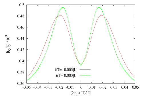
Figure 1: (Color online) Dependence of the heat current $I_{Q}$ on $x=(2\varepsilon_{d}+U)/|U|$ for $\delta T=\pm 0.003|U|$ and $\Gamma_{L}=2,\Gamma_{L}\cdot\Gamma_{R}=1$ in units of $|U|$. The temperature $T=0.005|U|$ and $I_{0}=e|U|/h$.

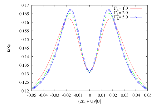
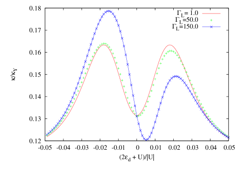
Figure 2: (Color online) Dependence of the thermal conductance $\kappa$ normalized to $\kappa_{U}=k_{B}|U|/h$ on $x=(2\varepsilon_{d}+U)/|U|$ for temperature $T=0.005|U|$, $\delta T=0.001|U|$. Figure a) is for strong junction asymmetry, while b) is for very large asymmetry.

IV Thermal rectification in a nonlinear transport

Outside the linear regime, i.e. for finite voltage bias $V$ and temperature difference between the electrodes, the transfer rates $W^{\lambda\lambda^{\prime}}_{n\rightarrow m}$ and $W^{\epsilon\lambda\lambda^{\prime}}_{n\rightarrow m}$ have to be calculated numerically. In the studies of charge conductance Koch interesting rectification properties of the device have been predicted. For strongly asymmetric coupling of the dot to the electrodes e.g. $\Gamma_{L}>>\Gamma_{R}$ the current $I_{e}$ is the asymmetric function of $x$ in the limit of $|eV|>>k_{B}T$. The intriguing question arises if similar rectification properties thermal-rect could be achieved in the heat flow. To answer this we have calculated the currents $I_{e}$ and $I_{Q}$ for general values of $V$ and $\delta T$. Formally both charge and heat currents depend on a voltage and a temperature difference

$$I_{e}=I_{e}(V,\delta T)$$ (20)

$$I_{Q}=I_{Q}(V,\delta T)\,.$$ (21)

As stated earlier the thermal conductance $\kappa$ is generally defined by $I_{Q}=-\kappa\delta T$ under the condition $I_{e}=0$. The condition of no current flow defines the thermoelectric power $S=-\left({V\over\delta T}\right)_{I_{e}=0}$, where $V$ is the voltage generated in the system by the temperature gradient. It provides the ’selconsistent value’ of the voltage to be used in equation (21). Introducing this into the equation for $I_{Q}$ we get

$$I_{Q}=I_{Q}(V=-S\delta T,\delta T)=-\kappa\delta T\,.$$ (22)

The last equality is our definition of the thermal conductance $\kappa$. In this section we measure all energies in units of $|U|$. The dependence of $\kappa$ on $x=2\varepsilon_{d}+U$ is shown in Fig. (2) for the temperature $T=0.005|U|$ and relatively small asymmetry of the junction, parametrised by the value of $\Gamma_{L}$ in the units of $|U|$, with $\Gamma_{L}\cdot\Gamma_{R}=1$ in the same units.

Calculating the currents we have assumed symmetric voltage and temperature difference with $V_{L,R}=\pm V/2$ and $T_{L/R}=T\pm\delta T/2$. For positive $\delta T$ the heat will normally flow from the left to the right lead. Thermal rectification can be defined thermal-rect as the dependence of the heat current $|I_{Q}|$ or the nonlinear thermal conductance $\kappa$ defined in Eq. (22) on the sign of temperature difference. Figure (1) shows the effect of heat rectification in the asymmetric molecular junction with $\Gamma_{L}/\Gamma_{R}=4$, the temperature $T=0.005|U|$ and two values of $\delta T=\pm 0.003|U|$. Due to phase space restrictions, which make the transition rates for two – electron processes $V$ and $\delta T$ dependent, the excess heat current $\delta I_{Q}=|I_{Q}(+\delta T)|-|I_{Q}(-\delta T)|$ depends on $x$ and changes sign around $|x|\approx 0.022|U|$ for a given set of parameters.

Both the heat flux and thermal conductance are the symmetric functions of $x$ for small values of asymmetry (see Fig. (2a)). However, for very strongly asymmetric junctions, the conductance starts to be the asymmetric function of the detuning parameter. This is shown in the Fig. (2b). The rectification coefficient defined as $\delta I_{Q}/I_{Q}$, changes sign as the function of $x$. For the parameters in figure (2a) it takes the maximal value of about 5%.

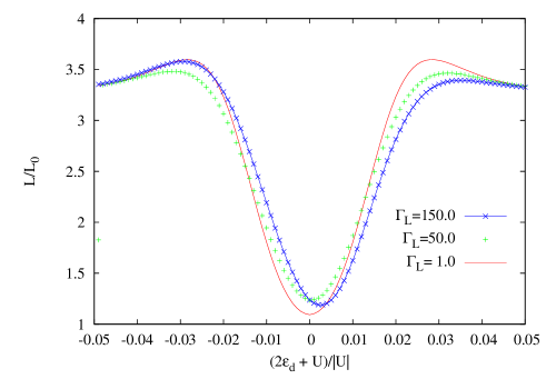
Figure 3: (Color online) Dependence of the Wiedemann-Franz ratio L normalized to its Fermi liquid value $L_{0}={\pi^{2}k^{2}_{B}\over 3e^{2}}$ on the parameter $x=2\varepsilon_{d}+U$ in units of $|U|$ for $T=0.005|U|$ and $\delta T=0.001|U|$. Couplings to the leads measured in units of $|U|$ are normalized by $\Gamma_{L}\cdot\Gamma_{R}=1$.

V Wiedemann-Franz ratio and quantization of electron thermal conductance

It has been predicted rego1998 that at low temperature the phononic thermal conductance of one dimensional dielectric wire is universally given by

$$\kappa_{0}=\left({\pi^{2}\over 3}\right){k^{2}_{B}\over h}T$$ (23)

leading to the universal, material and temperature independent ratio $\kappa_{0}/T={\pi^{2}\over 3}{k^{2}_{B}\over h}$, which sets a fundamental quantum limit on heat flow schwab2000 in an analogy to quantized charge conductance. The quantized value of the heat conductance is expected rego1998 in one-dimensional structures independently of the statistics of heat carriers. So this is valid for phonons, electrons and also particles with fractional statistics haldane 1991 . This result has been experimentally schwab2000 confirmed for phonons, electrons and photons.

It is an easy exercise to show that at $T\rightarrow 0$ the thermal conductance through our negative $U$ molecule reduces to

$$\kappa(T\rightarrow 0)=2{\Gamma_{L}\over|U|}{\Gamma_{R}\over|U|}\,{\pi^{2}\over 3}\,{k^{2}_{B}\over h}T\,{4\over(1+|x|)^{2}}\,.$$ (24)

Thermal conductance, which in the present context consists of only electron contribution is linear in temperature at low temperatures. The heat quantum, however, is not universal and depends on the coupling amplitudes $\Gamma_{L/R}$ and the dimensionless distance $x$ from the degeneracy point $2\epsilon_{d}+U=0$, measured in units of $|U|$. It is important to notice that the linear charge conductance at very low temperatures takes on the $T$ independent value

$$G_{0}(T=0)=2{\Gamma_{L}\over|U|}{\Gamma_{R}\over|U|}{4\over(1+|x|)^{2}}{e^{2}\over h}\,,$$ (25)

which ensures the validity of the Wiedemann-Franz (WF) ratio in this limit

$${\kappa(T\rightarrow 0)\over G(T\rightarrow 0)T}={\pi^{2}k^{2}_{B}\over 3e^{2}}=L_{0}\,,$$ (26)

being one of the signatures of the Fermi liquid.

For an arbitrary temperature and in the non-linear regime the above ratio of thermal to charge conductance takes on $T$, $\delta T$ and $x$ dependent values $L(x,T)={\kappa\over GT}$. The function $L(x,T)$ in units of the Lorenz number $L_{0}$ is shown in figure (3) for $T=0.005|U$ and $\delta T=0.001|U|$. At low $x$ it takes values close to 1, but for larger $x$ one observes strong departures from the Fermi liquid value $L_{0}$, like in the quantum dots with a large Coulomb interaction kubala 2008 . Its dependence on the coupling asymmetry is rather weak.

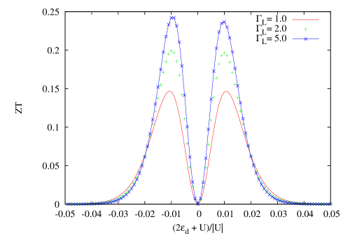
Figure 4: (Color online) Dependence of the nonlinear dimensionless figure of merit $ZT$ on the parameter $x=(2\varepsilon_{d}+U)/|U|$. The temperature $T=0.005|U|$ and $\delta T=-0.003|U|$ and the couplings are normalized by $\Gamma_{L}\cdot\Gamma_{R}=1$ in units of $|U|$.

We have also calculated the dimensionless figure of merit which indicates heat to voltage conversion efficiency of the device heremans2004 . It is usually defined as $ZT=GS^{2}T/\kappa$. For most devices thermal conductance contains both electron and phonon contributions. In the present geometry phonons do not contribute. The dependence of $ZT$ on $x$ for a few values of asymmetry is shown in Fig. (4). Its value increases with the asymmetry of the coupling and is a non-monotonous function of $x$. The maximum increases with the anisotropy of coupling as it is evident in the figure.

VI Summary

We have calculated the linear thermoelectric transport coefficients of the single electron molecular transistor in the limit of large electron-phonon coupling leading to a negative effective charging energy. In this limit the pair tunneling processes contribute mainly to charge and heat transport. Pair dominated transport shows strong departures from the Fermi liquid characteristics. We have found strong deviations from the Wiedemann-Franz law and a non-universal value of thermal conductance quantum. The thermal quantum i.e. the ratio $\kappa/T$ evaluated at a low temperature and the Lorentz function $L(x,T)$ depend on $x$ and asymmetry of the couplings. The thermoelectric figure of merit $ZT$ characterizes efficiency of the device for thermoelectric applications. This parameter takes on fairly low, albeit in general $x$ and $T$ dependent values for the negative $U$ quantum dot studied here. The maximal value of $ZT$ is about 0.25 for the strongly asymmetric junction.

Acknowledgmements: This work has been partially supported by the Ministry of Science and Education under the grant No. N202 1878 33 and the scientific network LFPPI.

References

- (1) J. Bardeen, L. Cooper, J. Schrieffer, Phys. Rev. 108, 1175 (1957).
- (2) R. Micnas, J. Ranninger and S. Robaszkiewicz Rev. Mod. Phys 62 113 (1990).
- (3) A.S Alexandrov, and N.F. Mott, Rep. Prog. Phys. 57 1197 (1994).
- (4) P. W. Anderson, Phys. Rev. Lett. 34, 953 (1975); R. A. Street and N. F. Mott, Phys. Rev. Lett. 35, 1293 (1975).
- (5) C.M. Varma, Phys. Rev. Lett. 61, 2713 (1988).
- (6) W. A. Harrison, Phys. Rev. B 74, 245128 (2006).
- (7) A. S. Alexandrov and N. F. Mott, Polarons and Bipolarons World Scientific, Singapore, 1995.
- (8) L. Jacak, P. Hawrylak and A. Wójs, Quantum Dots (New York: Springer) 1998.
- (9) M. Hohenadler and P.B. Littlewood, Phys. Rev. B 76 155122 (2007); M. Hohenadler and H. Fehske, J. Phys.: Cond. Matt. 19 255210 (2007).
- (10) J. Koch, M.E. Raikh and F von Oppen Phys. Rev. Lett. 96 056803 (2006).
- (11) A. S. Alexandrov, A. M. Bratkovsky, and P. E. Kornilovitch, Phys. Rev. B 65, 155209 (2002).
- (12) C. Holmqvist, D. Feinberg, and A. Zazunov, Phys. Rev. B 77, 054517 (2008).
- (13) M. Gierczak, and K.I. Wysokiński, J. Phys. Conf. Series, 104 12005 (2008).
- (14) M. Galperin, M. A. Ratner and A. Nitzan, J. Phys. Cond. Matt. 19, 103201 (2007).
- (15) J. Koch, E. Sela, Y. Oreg, and F. von Oppen, Phys. Rev. B 75, 195402 (2007).
- (16) J. R. Schrieffer and P.A. Wolff Phys. Rev. 149, 491 (1966).
- (17) H.-B. Schüttler and A. J. Fedro, Phys. Rev. B 38 9063 (1988).
- (18) We use the notion quantum dot (QD) in a loose sense to describe small central region of the considered structure, independently if it is defined in two dimensional electron gas, consists of a metallic or semiconducting grain or is in the form of a single molecule.
- (19) H. Bruus and K Flensberg Many-body quantum theory in condensed matter physics, Oxford Graduate Texts (New York: Oxford University Press) (2004), Ch. 10
- (20) G. D. Mahan, Many-Particle Physics, Plenum Press, New York and London (1981), Ch. 3.8.
- (21) The formula for linear thermopower derived previously gierczak2008 is expressed in terms of the integrals. Unfortunetly, the figures presented in that paper contain numerical error which lead to small departures (around 2% at the extrema of ) from the exact result.
- (22) G. Casati, Chaos 15, 015120 (2005); B. W. Li, L. Wang, G. Casati, Phys. Rev. Lett. 93, 184301 (2004); D. Segal, A. Nitzan, Phys. Rev. Lett. 94, 034301 (2005); M. Terraneo, M. Peyrard, G. Casati, Phys. Rev. Lett. 88, 094302 (2002); C.W. Chang, D. Okawa, A. Majumdar, and A. Zettl, Science 314, 1121 (2006); C. R. Otey, W.T. Lau, S. H. Fan, Phys. Rev. Lett. 104 154301 (2010); L. Wang and B. Li, Phys. World 21, 27 (2008); Chen XO, Dong B, Lei XL, Chin. Phys. Lett. 25 , 3032 (2008).
- (23) J. B. Pendry, J. Phys. A: Math. Gen. 16 2161 (1983); L. G. C. Rego and G. Kirczenow, Phys. Rev. Lett. 81, 232 (1998); Phys. Rev. B 59, 13080 (1999)
- (24) F. D. M. Haldane, Phys. Rev. Lett. 67, 937 (1991)
- (25) K. Schwab, E. A. Henriksen, J. M. Worlock, M. L. Roukes, Nature 404, 974 (2000); O. Chiatti, J.T. Nicholls, Y.Y. Proskuryakov, N. Lumpkin, I. Farrer, and D. A. Ritchie, Phys. Rev. Lett. 97, 056601 (2006); M. Meshke, W. Guichard and J. P. Pekola, Nature 444, 187 (2006).
- (26) B. Kubala, J. König, and J. Pekola, Phys. Rev. Lett. 100, 0066801 (2008).
- (27) J.P. Heremans, C.M. Thrush, and D.T. Morelli, Phys. Rev. B 70 115334 (2004); J.P. Heremans, Acta Physica Polonica 108, 609 (2005); M. Krawiec and K.I. Wysokiński, Phys. Rev. B 73, 075307 (2006); M. S. Dresselhaus, G. Chen, M. Y. Tang, R. G. Yang, H. Lee, D. Z. Wang, Z. F. Ren, J.-P. Fleurial, and P. Gogna, Adv. Mat. 19 1043 (2007).