Thermalisation of Local Observables in Small Hubbard Lattices
Abstract
We present a study of thermalisation of a small isolated Hubbard lattice cluster prepared in a pure state with a well-defined energy. We examine how a two-site subsystem of the lattice thermalises with the rest of the system as its environment. We explore numerically the existence of thermalisation over a range of system parameters, such as the interaction strength, system size and the strength of the coupling between the subsystem and the rest of the lattice. We find thermalisation over a wide range of parameters and that interactions are crucial for efficient thermalisation of small systems. We relate this thermalisation behaviour to the eigenstate thermalisation hypothesis and quantify numerically the extent to which eigenstate thermalisation holds. We also verify our numerical results theoretically with the help of previously established results from random matrix theory for the local density of states, particularly the finite-size scaling for the onset of thermalisation.
pacs:
03.65.-w, 05.30.Ch, 05.30.-dpacs:
05.30.-d,03.75.-b,67.85.-d,67.85.LmI Introduction
Understanding the quantum origins of statistical mechanics has seen renewed interest over the last few years, in part motivated by experimental progress in degenerate atomic gases, but also due to independent theoretical advances Cazalilla and Rigol (2010); Polkovnikov et al. (2011); Yukalov (2011); Gemmer et al. (2005). The central question is as follows. Consider a closed quantum system prepared in a pure quantum state. Does it evolve in time to a thermal state? If so, in what sense is it a thermal state?
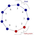
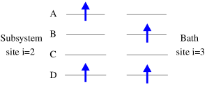
In this paper, we focus on observables that are local to a subsystem of the full system. Thus, we discuss the ‘thermalisation’ of this subsystem with the rest of the system as a bath (see Fig. 1). We will discuss the conditions for the eventual thermalisation of this subsystem. This has been studied in many systems Saito et al. (1996); Yuan et al. (2009); *Jin2010; Henrich et al. (2005); Gogolin et al. (2011); Cho and Kim (2010) and we will study a system of interacting fermions in this context. The picture of a local subsystem in a closed system also naturally makes contact with the conventional framework of statistical mechanics where thermal equilibrium is achieved by a weak coupling between a system and its environment.

Thermalisation in closed quantum systems has been shown to have its origins in entanglement. To be specific, let us consider a composite system with a Hamiltonian where describes the dynamics of subsystem () and the bath () respectively while couples the subsystem to the bath. The exact eigenstates of this Hamiltonian are typically superpositions of many eigenstates of the decoupled system () which are products of the subsystem and bath states: . The idea of ‘canonical typicality’ Tasaki (1998); Goldstein et al. (2006); Popescu et al. (2006); Reimann (2007); *Reimann2008; Linden et al. (2009) states that almost any pure state composed of many energy eigenstates within a narrow energy window will give rise to a canonical distribution for the measurements of local or few-body observables within the subsystem. This emerges because the pure state is an entangled combination of subsystem and bath eigenstates. We will consider in this paper a system prepared initially at time in a pure state that is a product state of the subsystem and bath states. Such a state is typically a superposition of many closed-system eigenstates: . While this initial state is special and cannot be considered as ‘typical’, we expect the wavefunction will, in general, evolve in time () towards a state that falls into the domain where canonical typicality applies. The sufficient conditions for this to occur have discussed in recent papers Linden et al. (2009); Gogolin (2010); Lychkovskiy (2010). In this paper, we will investigate conditions for thermalisation in a small Hubbard-model system.
An alternative view is the eigenstate thermalisation hypothesis Deutsch (1991); Srednicki (1994); Rigol et al. (2008) (ETH). The time evolution of any few-body observable involves the interference of eigenstates at different frequencies: where is the energy of the eigenstates and . The eigenstate thermalisation hypothesis says that destructive interference removes all terms and that
| (1) |
where the right-hand side denotes the thermal average of when the total system has energy . This paints a very different picture of thermalisation compared to the scenario for classical statistical mechanics where states diffuse ergodically through phase space constrained by energy conservation.
These concepts are powerful because they guarantee thermalisation for closed quantum systems. They depend crucially on the very high dimensionality of the Hilbert space of quantum states. In this paper, we aim to gain insight into these ideas by testing the limits of these hypotheses in terms of the breakdown of thermalisation for a small closed quantum system. We take our motivation from cold atom experiments with optical lattices and single-site addressibility Sherson et al. (2010); Bakr et al. (2010). We choose a lattice system of interacting fermions in a normal metallic state. In particular, we present a study of the thermalisation of a composite system consisting of a 2-site subsystem and a -site bath in a one-dimensional Hubbard ring. We avoid the issue of integrability and the generalised Gibbs ensemble Rigol et al. (2007) by choosing parameters such that it is a non-integrable system.
In order to study the thermalisation of the subsystem, we need to calculate the long-time behaviour of reduced density matrix of the subsystem:
| (2) |
where TrB denotes a trace over the bath degrees of freedom. A thermalised system corresponds to a diagonal reduced density matrix with diagonal elements given by the Gibbs distribution. We explore whether thermalisation occurs over a range of system parameters. We find numerically (section III) that thermalisation occurs in surprisingly small systems. For a system of a given size, there is a threshold for the onset of thermalisation, both in terms of the coupling strength and the interaction strength. In particular, we study the size dependence of the threshold that the coupling strength has to exceed to achieve thermalisation. We demonstrate that this threshold for thermalisation agrees with the ETH criterion (1) for thermalisation (sections III.7). Indeed, a theoretical threshold determined from the ETH criterion has the same size dependence as the empirical (section V.1). We also argue that both of these thresholds mark the onset of non-perturbative mixing of eigenstates due to the subsystem-bath coupling (at a threshold ).
From a separate perspective Deutsch (1991); Srednicki (1994), we can study the thermalisation process in terms of the statistics of the eigenstates. We study the statistics of the overlap of the eigenstates of the coupled system with the eigenstates of the decoupled system which are product states . Interestingly, at weak subsystem-bath coupling where the onset of thermalisation occurs, the distribution for the overlaps fits a hyperbolic secant distribution (section IV.1). This is in contrast to previous conjectures Berry (1977); Deutsch (1991); Srednicki (1994) from random matrix theory which suggest that these types of overlaps should follow a Normal distribution at weak coupling.
Using our results for the overlap distribution, we show numerically (section III.7) that the eigenstate thermalisation hypothesis (1) holds for the projection operator which projects onto the subsystem state in the parameter regime where the subsystem is thermalised. This can be explained theoretically (section IV.2) using known results for the variance of the overlap distribution. This observation for then leads directly to a thermalised reduced density matrix. (See section III.2.)
In this paper, we also highlight the importance to thermalisation of the strength of interaction within the bath. We find that, at least for our small bath and subsystem, a finite interaction strength is needed for thermalisation. This is consistent with the expectation that thermalisation is aided by inelastic scattering in the bath.
We point out that, although we have focussed on the thermalisation of a spatially local subsystem, one can also study the thermalisation of few-body observables over the entire system. This has been studied particularly in the context of quantum quenches in a variety of systems Rigol et al. (2008); Rigol and Santos (2010); Ji and Fine (2011); *Fine2009; Canovi et al. (2011); Lesanovsky et al. (2010); *Ates2012, including integrable systems Kinoshita et al. (2006); Rigol et al. (2007); Eckstein and Kollar (2008); Sotiriadis et al. (2009); Calabrese et al. (2011); Cassidy et al. (2011); Poilblanc (2011). Moreover, one can discuss the dynamics of the relaxation towards a thermal state Jensen and Shankar (1985); Eckstein et al. (2009); Genway et al. (2010); Lesanovsky et al. (2010); Ates et al. (2012); Kollar et al. (2011). Both of these issues are beyond the scope of this paper.
This paper proceeds as follows. The following section introduces the Hubbard model we study, discusses how the system is prepared initially and provides a framework for studying thermalisation. In Section III, we present a comprehensive set of results for the thermalisation of two-site subsystems in small Hubbard rings. We consider the effects of subsystem-bath coupling strength on thermalisation and link these results to eigenstate thermalisation. We further demonstrate the role of interactions between fermions before exploring system size dependence and, finally, the energy width of the initial prepared state. Section IV introduces results from random matrix theory concerning the nature of the eigenstates of the coupled system. From these, we review the arguments leading to eigenstate thermalisation Srednicki (1994) and derive the scaling behaviour associated with the closeness to perfect eigenstate thermalisation. In Section V, we present an account of system-size scaling by considering a threshold for non-perturbative mixing of uncoupled composite eigenstates for the cases of both interacting and non-interacting fermions. In Section VI, we discuss implications for experiments. Finally, in Section VII, we give our conclusions.
II The Model and Theoretical Framework
We will consider closed quantum systems with unitary time evolution. The system is prepared in an initial state which evolves in time under the influence of the Hamiltonian . In this section, we discuss the specific model studied in this work and our choice of initial states. Since we will investigate thermalisation of a subsystem of this closed system, we will also discuss our criteria for a thermal state.
II.1 Hubbard Hamiltonian
We divide the system into a local subsystem () and a bath (). The subsystem (bath) is described by a Hamiltonian () acting on the subsystem (bath) Hilbert space. Let us denote the subsystem (bath) eigenstates as () with energies (). The subsystem and bath are coupled by a Hamiltonian . We will use as a tunable parameter to control the strength of this coupling. At , the eigenstates are products of subsystem and bath eigenstates, , with energies . At non-zero , the eigenstates are in general entangled with respect to the subsystem-bath partition. We denote these composite eigenstates by (using an uppercase index) and their energies by .
In this work, we focus on the Hubbard model away from half filling as a simple model of interacting fermions. More specifically, we consist of a two-site subsystem in an -site Hubbard ring of fermions such that the Hamiltonian takes the form with
| (3) |
where is a creation operator for a fermion with spin at site and is the number operator on site with spin . This Hamiltonian describes a ring with the subsystem sites and bath sites to with two links between the subsystem and the bath. Note that, in the case of , the Hamiltonian describes an homogeneous ring. We choose the hopping integrals , with to remove level degeneracies associated with spin rotation symmetry. (We will use as the unit of energy.) Breaking spin symmetry and the presence, in general, of modified hopping integrals between sites and , as well as between sites and make this system non-integrable for non-zero .

The total particle number, , and spin component, , are conserved in addition to the total energy of the composite system. In the numerical results we present, we consider lattices with up to sites and with 8 fermions of total spin . The two-site subsystem has eigenstates and the 7-site bath has 8281 eigenstates, while the composite 9-site system has a total of states and an average level spacing .
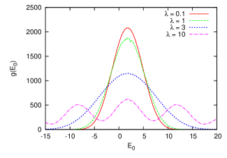
The spectrum of the composite system has a smooth quasi-continuous density of states for a range of and . This is illustrated in Figs. 3 and 4. The centre of the spectrum is located at . The spectrum develops peaks for large and . In the case of , we attribute this to single-particle states with a large energy splitting proportional on the two links connecting the subsystem and bath. For , we attribute the peaks to a large energy gap to doubly-occupied sites (sometimes referred to an ‘upper Hubbard band’ in the theory of strongly electron systems or doublons in the cold atoms literature).
II.2 Initial States
Throughout this work, we consider the composite system to be prepared in a pure state which is a product state of a subsystem state and a bath state:
| (4) |
The initial subsystem state, , can be, for example, which is prepared with antiparallel spins on sites and 2 of the lattice. The initial bath state contains a linear combination of bath eigenstates . These bath states are chosen to be within an energy window of bath states such that . The energy window has a width in energy of (specified by the state indices in the range ). Unless stated otherwise, we choose which is small on the scale of variations in the density of states. For a 7-site bath, this window contains about 100 bath eigenstates.
As the system evolves in time, the state of the subsystem can be described by the reduced density matrix (RDM) as defined in equation (2). We will study the reduced density matrix elements using the subsystem eigenstates as the basis: . We obtain the wavefunction of the composite system using the eigenstates and energy eigenvalues from the exact diagonalisation of the Hamiltonian :
| (5) |
II.3 Thermalisation
To assess whether the subsystem reaches a thermal state, we must be more precise about the criteria for a thermal state. We start with the conventional definition of thermal equilibrium in the canonical ensemble. To define this ‘canonical thermal state’, , of the subsystem, we set up the composite system at a total energy in a microcanonical mixed state and consider the regime where the coupling between the subsystem and the bath is negligible. In this way, the thermal state of the subsystem may be determined by counting bath states in an energy window, conserving the total energy and the global and particle number . The reduced density matrix is diagonal and is given by :
| (6) |
where is the number of bath states with fermions of spin in a window of width centred on energy . This thermal RDM is a function of , and , arising from the global conservation laws of the system. For fixed and and for a range of subsystem energies small compared with features in the density of states, the smooth density of states allows us to write the RDM in the Boltzmann form , with the inverse temperature given by
| (7) |
We can in principle deduce a chemical potential and Zeeman field by considering variations in and . However, we are considering small systems where the discreteness of these quantities cannot be ignored and is not a smooth distribution of and . Nevertheless, Eq. (6) may be used to specify a thermal state of the subsystem for, in principle, any bath size.
We note that such a Gibbs-like distribution has just three parameters, differing from the ‘generalised Gibbs distribution’ for integrable systems Rigol et al. (2007, 2008); Cassidy et al. (2011), where the number of parameters extends with system size.
Let us now turn to the RDM that we obtain from the unitary evolution from an initial pure state. We will be examining the behaviour of the RDM at long times. It is useful to define the time average:
| (8) |
If the reduced density matrix reaches a steady state at long times, this state will be equal to the time average . We expect this to become diagonal. Using Eq. (2), we see that the diagonal elements of the RDM are given by
| (9) |
Averaging over time for long times identifies with . Since we have lifted all symmetry-related degeneracies, this also identifies states and in the sum above (barring accidental degeneracies). So we see that
| (10) |
The operator projects from the composite Hilbert space on to the subsystem state by tracing over bath states.
The coefficients contain the information about the initial state. However, this steady state may still be very close to a state which is independent of initial conditions. A sufficient ondition is given by the ‘eigenstate thermalisation hypothesis’ Rigol et al. (2008). Recall that from Eq. (4) our initial state has been set up within a narrow energy window. So, the overlap of should be only non-zero in a window of eigenenergies. (We will give a more quantitative discussion of the width of this window in Section IV.1.) The eigenstate thermalisation hypothesis assumes that for a system with composite energy depends only weakly on the choice of in this window of eigenenergies. This allows us to replace by its average value over the eigenenergy window. In that case, . Thus, we see that the steady state may indeed be independent of initial conditions.
Furthermore, if is close to the value for the canonical ensemble (6), then Eq. (II.3) can be written as . Thus, will be close to the canonical thermal state for any initial state with a definite energy.
In summary, we break down the question of whether the subsystem thermalises into four criteria similar to the ones in Ref. Linden et al. (2009). Our criteria are
-
1.
Firstly, we should establish that the reduced density matrix reaches a steady state at long times.
-
2.
The steady state should be diagonal in the subsystem energy eigenbasis with all off-diagonal elements falling to zero for long times. This demonstrates a loss of quantum coherence.
-
3.
This steady state should have no memory of the initial state, such as the precise way in which the subsystem or the bath is prepared.
-
4.
Finally, we ask if this steady state is close to the canonical thermal state . If this is the case, we will say the system exhibits ‘canonical thermalisation’.
We are leaving open the possibility that the subsystem reaches a steady state with no memory of the initial state, but does not resemble the canonical thermal state. This may be possible since the canonical state has been derived assuming the bath states are unperturbed by the coupling with the subsystem which may not hold in the small quantum systems studied here when the coupling is of order unity.
We explore these questions with numerical studies of the Hubbard Hamiltonian in the following section. We will discuss the more sophisticated picture of the eigenstate thermalisation hypothesis separately in Section IV.
III Numerical Results
III.1 Long time behaviour
We proceed to demonstrate that the first two criteria for thermalisation listed at the end of Section II.3) are met for a range of system parameters. These requirements are that the reduced density matrix should approach a steady state at long times, with its off-diagonal elements falling to zero.
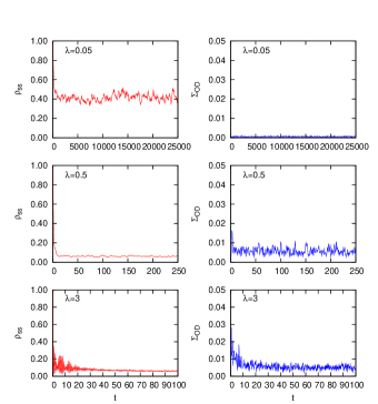
Initial states of the form in Eq. (4) were constructed with the initial subsystem state . It was found that evolving in time under the Hamiltonian results in almost steady states for a wide range of , provided the composite energy is not close to the edge of the spectrum. With interaction strength and bath width , this range is for a composite energy . Examples are shown in the left panel in Fig. 5. This shows the relaxation of the diagonal element of corresponding to the initial-state occupation probability for couplings , 0.5 and 3. The dynamics of the relaxation is fast and featureless for up to 1. The temporal fluctuations around the long-time steady state are small at this energy . In fact, if we use an energy close to the centre of the spectrum of the composite system (), temporal fluctuations are even smaller for a given . On the other hand, for an energy closer to the edges of the spectrum, the density of states is small so that few composite states construct the initial state. The presence of only a few frequencies in the time evolution limits the closeness to a steady state achievable.
We see beating oscillations at which we attribute to the strongly split single-particle states at the two subsystem-bath links at large . Indeed, for even larger , no longer reaches a steady state, and the frequency spectrum begins to show peaks at frequencies which are integer multiples of .
Let us now investigate the second condition for thermalisation that off-diagonal elements fall to zero with only small temporal fluctuations, as predicted in Gogolin (2010). We compute the root-mean-square sum of these off-diagonal elements:
| (11) |
This is shown in the right panel of Fig. 5. By construction, is larger than any single off-diagonal element. We see that the effect of off-diagonal elements can be neglected at long times: is, with decreasing , shown to be from down to times smaller than each diagonal element.
Having established that, within a range of coupling strengths, the subsystem RDM does reach a diagonal steady state with only small temporal fluctuations, we will now use Eq. (II.3) to compute the steady-state form without explicitly computing at many times and taking a time average. This is less computationally expensive and provides a definitive long-time subsystem state without the need for numerically averaging out small temporal fluctuations.
We will now proceed to explore two further requirements of thermalisation: these are the extent of initial-state independence and closeness to the thermal state . The effective temperature of the subsystem may also be estimated from .
III.2 Quantifying Thermalisation
Next we develop measures to characterise the extent to which the third and fourth of our thermalisation criteria, listed in Section II.3, are met.
Criterion 3 in Section II.3 is concerned with the loss of memory of the initial state at long times. To quantify the variation in the steady state due to different initial states, we introduce the measure which measures the root-mean-square variation in diagonal reduced density matrix elements for different initial subsystem states:
| (12) |
with denoting an average over all initial states in the subsystem Fock basis, as in Eq. (13). We expect to be small when the long-time steady state no longer depends on how the system was initially prepared.
Criterion 4 in Section II.3 addresses the closeness of the subsystem state at long times to the canonical thermal state . We quantify this with the quantity , defined as:
| (13) |
Here, denotes an average over all initial states in the subsystem Fock basis (eigenstates at ). As such, this is a measure of the average distance to the thermal state, , for the set of initial subsystem states spins localised on the lattice sites. It is a special case of a more general distance measure Linden et al. (2009), , which equals in the case where the elements of in the subsystem eigenbasis form diagonal matrices. As established above, this is the case for . Within this range, we may interpret as the probability, upon making measurements on the subsystem, that could be distinguished from Popescu et al. (2006).
From the definitions of these two measures, it is clear that if is large then is necessarily large too: if there is a large variation in for different initial states, many of these states must be far from the uniquely defined canonical thermal state . Conversely, it is possible for to be large with small, because the subsystem may relax consistently to a state other than the canonical state .
We will also compute the von Neumann entropy of the subsystem. Because off-diagonal elements of are virtually zero at long times even for very small , we introduce an initial-state-averaged subsystem entropy for the equilibrium state, which we define by
| (14) |
where denotes an average over all initial subsystem states in the subsystem Fock basis.
We would also like to characterise subsystems showing thermalisation with an effective temperature. As discussed in Section II.3, if we consider the subsystem at a given particle number and spin , we expect the steady-state RDM, , to approach the Boltzmann form (7) for if the subsystem relaxes to the canonical thermal state . Therefore, we extract an effective temperature from the RDM, , of the steady states that we find using a least-squares fit to the form
| (15) |
We will focus on the four-state subsector with and because it is the subsector with the largest number of bath states. Note that it is possible that we can have a good fit to this form with an effective temperature even if the steady state is not close to the canonical state .
III.3 The Role of Coupling Strength
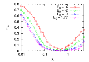
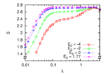
In the previous section, we discussed how we measure the memory of the initial conditions () in the steady state, closeness () to the canonical thermal state, the effective subsystem temperature () and the entropy () of the subsystem. We will now discuss how these measures of thermalisation change over a broad range of subsystem-bath coupling strengths . We show results at different total energies between and 1.77.
In Fig. 6, we present our results for , and as a function of the coupling strength (for a system with and an initial state of bath width ). Our results for demonstrate that the subsystem reaches a steady state with little dependence on initial conditions over a wide range of coupling strengths . We see significant dependence on initial state beyond this range, at both small and large . Moreover, our results for show that the subsystem reaches the canonical state over a similar, albeit slightly narrower, range of coupling strengths. Outside this range, the long-time steady state shows strong deviation from the canonical state.

In the coupling range where and are both small, we find that the entropy reaches a plateau as a function of . Beyond this range at low , the subsystem entropy drops with decreasing . This is consistent with the subsystem retaining information of its initial conditions. On the other hand, the entropy rises when is increased beyond the plateau. The asymmetry between low and high coupling indicates that the departure from thermalisation at small and large have different physical origins, as we discuss later. The behaviour of the subsystem reduced density matrix as a function of is summarised by the schematic diagram in Fig. 7 for the range of energies shown in Fig. 6.

We show in Fig. 8 the effective temperature extracted at different energies using the fit in Eq. (15). We include only the range of coupling strengths where the fit is reasonable. It is noteworthy that our results with two lowest energies, and , show effective temperatures close to the degeneracy temperature, approximately for this Hubbard system near half filling.
We have not shown for the highest energy we used, . This energy corresponds to the centre of the energy spectrum for all plotted. At this energy, all the states of the subsystem have nearly equal statistical weight at this energy. In other words, the effective temperature is nearly infinite. This is also reflected in the subsystem entropy (Fig. 6) which is close to at , as expected for our 16-state subsystem at high temperatures.
For systems exhibiting canonical thermalisation (small ), the effective temperature is approximately independent of the coupling strength up to . In fact, this effective temperature is close to the canonical temperature defined in Eq. (7) by counting bath states in the limit of , as reported in Genway et al. (2010). As already mentioned, we find in this regime that the subsystem entropy (Fig. 6) is also roughly independent of .
We will now turn to the crossover from non-thermalisation to thermalisation as we increase the coupling strength from zero. We can choose a rough measure of the threshold, , for this crossover as the coupling strength at which drops below 25%. Alternatively, we can use the coupling strength at which the subsystem entropy reaches a plateau in Fig. 6. At , we find . At the lower energy , is higher at approximately 0.1. At the energy corresponding to the centre of the spectrum, is smallest at 0.03. The crossover between memory and lack of memory of the initial state also occurs around this characteristic coupling . (We discuss this criterion further in Section V.) That thermalisation does not occur for small coupling strengths is because of the finite level spacing, , in the finite-size bath. Physical intuition might suggest that subsystem-bath couplings, however weak, allow relaxation in subsystems. This is a reasonable assertion for systems with macroscopic baths where the bath spectrum is quasi-continuous. However, for a small system with a non-zero level spacing at weak coupling, the eigenstates of the composite system may only be slightly perturbed from the decoupled subsystem-bath product states if the typical matrix elements mixing these product states are small: . In this weak-coupling limit, thermalisation cannot occur from an initial subsystem state , when the composite eigenstates are all close to product states of the form . The system would retain strong memory of the initial state. Therefore, we expect a non-zero threshold for thermalisation for a finite system. We will examine more quantitatively the overlap of the composite eigenstates with the decoupled product states in Section IV and we will compare the empirical extracted here with a theoretical estimate in Section IV.2.
Let us now turn to the strong-coupling regime of . As already discussed in Section III.1, the system does not reach a steady state at very high , and so it is not thermalised. We believe that this is a boundary effect in the sense that the dynamics in our ‘subsystem’ consisting of sites 1 and 2 become altered at very large because of the very large hopping on the links between sites 2 and 3 and between sites 1 and . As already discussed in Section II.1, single-particle states localised on these links become visible as a feature the composite density of states at (Fig. 3). We believe that the four sites (,1,2,3) will thermalise as a cluster in the sense that it has a canonical reduced density matrix, provided that the bath of size is sufficiently large. Nevertheless, since the eigenstates of the two-site cluster and the four-site cluster are very different at large , the thermalisation of the four-site cluster does not imply a diagonal RDM for the two-site cluster. In any case, we wish to make the point that this lack of thermalisation at large coupling is qualitatively different in origin from the lack of thermalisation at small coupling.
It is interesting to examine more closely the departure from thermalisation as we increase in the range of between 1 and 3 for (see in Fig. 6). In this crossover region, we find steady states that have lost memory of the initial state (small ) but these states deviate from the canonical thermal state , as can be seen in a rising as is increased beyond unity. Moreover, the RDM has a reasonable fit to the Boltzmann form (15), although the fitted temperature departs significantly from the canonical temperature (7). One can say that the system is still in an ‘effective’ thermal state in this crossover regime. We will return to this in Section III.7.
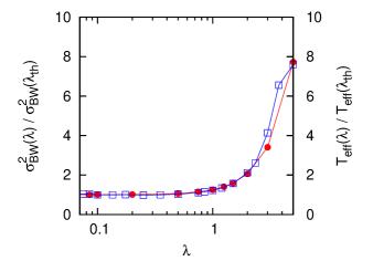
Interestingly, we observe that this crossover regime tracks closely a decrease in the density of states of the composite system. The density of states (Fig. 3) can be approximated as a Gaussian:
| (16) |
where is the energy of the band centre, and can be used as a measure of the width of the Gaussian. We see in Fig. 9 that rises sharply as we increase beyond unity, similar to the behaviour of the fitted effective temperature (Fig. 6). In fact, , as seen in Fig. 9 where we show the two quantities normalised to their (-independent) values at small . Note that, at weak coupling and at fixed energy , the derivative
| (17) |
can be associated with the inverse temperature of a bath of size . In other words, it appears that the effective temperature of the subsystem is better described by the canonical temperature of the whole system, instead of just the bath. This result is not surprising in this regime where the coupling of our 2-site subsystem to the chain is of order unity, since the distinction between subsystem and bath is blurred.
III.4 Dependence on Interaction Strength
We now turn to the effects of the particle-particle interaction strength, , on thermalisation. In the results which follow, the coupling strength is fixed, as previously, at and we will also fix the bath width at . The energy of the composite system, , will be fixed such that it is always at the peak in the centre of the composite spectrum, at . This is necessary since the shape of the spectrum is a strong function of and the density of states at a given energy can vary significantly. The effects of the interaction strength on the composite density of states are shown in Fig. 4. We find that for , peaks separated by appear. If comparisons were to be made between different for initial states at fixed , the features in the density of states which evolve with would introduce unwanted artefacts. Even in the centre of the spectrum, it should be noted that there is a fall in the density of states at the central peak at , which occurs over a range due to an overall broadening of the density of states (see Fig. 3).
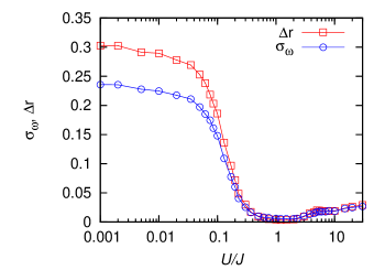
To measure thermalisation at different , we will again employ the measures and as defined in Eqs. (12) and (13). The effective temperature is not shown since the initial-state energy is at a maximum in the density of states which corresponds to infinite subsystem effective temperature. In Fig. 10, we demonstrate that thermalisation, independent of the initial state, is found for . There is a broad minimum in plots of both and , defined by the lack of thermalisation at small and a small increase in the plotted quantities over the range .
The slight increase in and above coincides with the falling density of states in the centre of the spectrum shown in Fig. 3. So, the increase may be partly associated with the reduction in the number of states in the fixed bath window of our initial state.
The behaviour at small cannot be similarly related to the density of states. However when , the nature of the coupling is very different because the bath states are Slater determinants single-particle states. The single-particle level spacing is large compared to if . So, we expect that thermalisation is poor for small non-interacting systems. In other words, for small , we need larger system sizes to observe thermalisation. We will present our data for different system sizes in the next subsection (Fig. 12).
III.5 System Size Dependence
It is interesting to study thermalisation as a function of system size. Owing to the exponential dependence of the Hilbert-space dimension on lattice size, it is not possible to find the full spectrum of large lattice. We will instead concentrate on the loss of thermalisation as we reduce the system size. If we use even smaller systems, reducing the number of sites rapidly leads to Hilbert spaces so small that thermalisation is not observed at all. Nevertheless, our results show that thermalisation is possible in surprisingly small systems, as long as so that the system is not close to the non-interacting limit, and as long as the density of states is not too low. To attempt to see some effects of reducing system size on thermalisation, we consider composite states prepared with energies in the centre of the band where the density of states is highest. As with our studies of the effects of interaction strength, this also eliminates unwanted effects due to the changing bandwidth with system size.
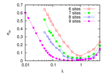
First of all, let us consider how our results in Section III.3 for the dependence on coupling strength changes with system size. Shown in Fig. 11 are plots of for different lattice sizes down to six sites. In each case, the subsystem size was fixed at two sites and the initial bath width was fixed at . Interestingly, for , thermalisation is maintained down to a four-site bath. However, the range of couplings over which thermalisation occurs is greatly reduced. We return to system-size scaling in section V.
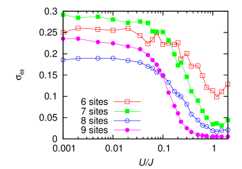
We can also see how our results in Section III.4 for the dependence on interaction strength, , change with system size. We see in Fig. 12 that the larger systems have a wider range of interaction strengths over which the system approaches the canonical thermal state (small ). Moreover, is lower for larger systems at a given . This is consistent with our expectation that weakly-interacting systems require larger system sizes for thermalisation. We will explore system-size scaling in Section V.
III.6 Dependence on Initial Bath State
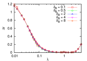

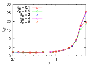
The thermal state should not depend on the microscopic details of the initial bath state. We will now demonstrate that the thermalisation behaviour found at long times is independent of the initial bath state. More specifically, we will vary the energy width of the initial bath state. For all of the numerical results presented thus far, we have considered initial states of the form (4) where the initial bath state is a pure state, with components in the bath eigenbasis non-zero only in a window of width . This was chosen because it is small compared with changes in the density of states. In Fig. 13, we show plots of , and against for values of spanning almost two orders of magnitude. In other words, these are results for vastly different bath states with the only constraint that they should be centered at the same energy.
We find that the thermalisation behaviour is essentially -independent for a broad range in . Remarkably even up to , approximately half of the width of the composite eigenspectrum, we see makes virtually no difference to the initial-state memory, quantified by , and the effective temperature . The distance to the thermal state at long times is modified slightly by choosing a very large , but it should be noted that is itself dependent on the energy width of the state when this becomes large on the scale of changes in the density of states.
Conversely, we can make so small that there is just one initial bath eigenstate in the initial product state and virtually identical behaviour to Fig. 13 is seen when . However, for smaller values of , fluctuations appear as a function of , thus necessitating a finite .
III.7 Eigenstate Thermalisation
We now discuss our results in relation to the eigenstate thermalisation hypothesis (ETH). As discussed in Section II.3, this hypothesis requires the eigenstate expectation values of the subsystem projection operator, , (defined in Eq. (II.3)) to depend only weakly on the exact choice of the eigenstate .
We expect ETH to be valid in the regime where we found thermalisation in the previous sections — for , this regime covers a wide range of coupling strengths, , with exhibiting behaviour closest to the canonical picture of thermalisation. So, we will now study the dependence of eigenstate projections on the coupling strength at . We will focus on the projection on to the ground state of the subsystem in the (, ) sector at .
‘Perfect eigenstate thermalisation’ corresponds to the projection values forming a smooth quasi-continuous function of composite eigenenergy . When this occurs, complete independence of the initial subsystem state exists. Fig. 14 shows histograms of . We see that there is some scatter in for different eigenstates that are close together in energy. There is the least scatter when the subsystem is closest to the canonical thermal state (small and ) at for . Greater scatter in the values of is found when the system starts to lose thermalisation (by our other measures of thermalisation), at small and at large .
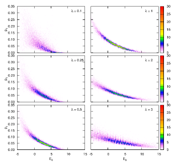
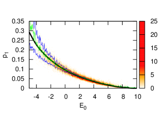
Let us examine the case of at more closely. This shows little scatter, and hence good eigenstate thermalisation, over a wide range of energies. We quantify the extent to which eigenstate thermalisation holds by measuring the mean and the standard deviation, , of the scattered values in each vertical column of histogram bins on the plot in Fig. 14. This is computed using values within an energy window of . (This reduces the fluctuations in the measured .) Fig. 15 shows the positions of the mean values of and the positions of from the mean. We see that there is indeed good agreement between the mean eigenstate projections at any particular energy and the canonical thermal value as defined in (6).
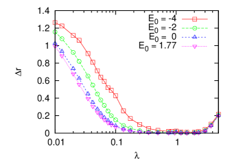
Let us now study the departure from eigenstate thermalisation, measuring it by the increase in the scatter in the eigenstate projection values. To reduce any bias due to changes in the density of composite states with , we used eigenstates at the energy which is near the maximum in the density of states for all coupling strengths considered here. The results are presented in Fig. 16. First of all, we observe that a minimum in indeed occurs over the same range of coupling strengths where other measures of thermalisation also show that the subsystem is close to a canonical thermal state. Secondly, we find that, as the subsystem departs from eigenstate thermalisation at low coupling strengths, the increase in with decreasing obeys the relationship
| (18) |
We will discuss this scaling in Section IV.2.
We also lose eigenstate thermalisation if we increase the coupling strength to . As discussed before, we believe that this is a particular feature of our model where the properties of the coupling dominate the Hamiltonian.
Finally, recall that we found in Section III.3 that, as is increased beyond unity at , the steady state of the subsystem departs from the canonical thermal state but the RDM follows a good fit to the Boltzmann form. This seems to indicate that the subsystem is in an effective thermal state that is non-canonical. We can see an indication of this crossover regime in Fig. 14 for , where the scatter in the eigenstate projections is still relatively low, but the mean eigenstate projections as a function of depart significantly from the canonical thermal value , in contrast to the case at (Fig. 15).
In summary, we have shown that eigenstate thermalisation holds and agrees well with other measures of thermalisation. We will demonstrate in Section IV.2 that the statistical behaviour of the eigenstate projections is consistent with a simple model of the eigenstates as random vectors in the basis of the subsystem-bath product states .

IV Eigenstate overlaps and the Eigenstate Thermalisation Hypothesis
In Section III.7, we showed that the eigenstate thermalisation hypothesis holds over a wide range of parameters for our Hubbard-model system. Deutsch Deutsch (1991) and Srednicki Srednicki (1994) have suggested that eigenstate thermalisation occurs if the composite system is quantum chaotic. This was demonstrated theoretically for weak subsystem-bath coupling using results for the eigenstates of generic (random) Hamiltonians. In this section, we summarise these arguments and demonstrate numerically their agreement with our results for our Hubbard-model lattice. We will then use this framework to explain the dependence of eigenstate thermalisaton on the coupling strength discussed in section III.7, namely the scaling of the spread of eigenstate projections, , with coupling strength for .
IV.1 The Overlap Distribution and the Local Density of States
To be more specific, eigenstate thermalisation is concerned with the eigenstate projections . So, we need to understand the overlap of the eigenstates of the composite system at non-zero coupling with the eigenstates of the decoupled system at . As for the eigenstate projections , the overlaps will fluctuate if we change or . However, we can study averages over energy windows that are narrow on the scale of variation in the density of states but contain enough states to smooth out fast fluctuations.
The overlaps themselves are not invariant under a global gauge transformation and so should have mean zero. Let us consider first the squared overlap whose average is the variance of the overlaps. This can be interpreted as the weight of the product state at energy in the decomposition of the eigenstate at energy using all the product states as the basis. In this picture of the composite eigenstate in energy space, is called the ‘local density of states’.
We now discuss some known results for the local density of states. For a coupling between subsystem and bath, we expect that an eigenstate at will consist mainly of product states with energies close to . If the coupling is not strong (), the energy range should scale with the strength of the coupling matrix elements where is the product state corresponding to in the limit . To leading order in , this can be written as . In this weak-coupling regime, we expect that the density of state of the bath spectrum is nearly constant over this range. Then, the mean value, , should be a strong function of the energy difference , but has only a weak dependence on and separately. For a generic random coupling, we expect a Lorentzian form in the dependence on the energy difference:
| (19) | ||||
where is the density of states of the composite system evaluated at the total energy , taken to be approximately constant over the energy width of this Lorentzian so that in this range of energy. It may be related to straightforward perturbation theoretic results Kottos and Cohen (2001); *Cohen2000; *Hiller2006 to second order in . This result was originally established Wigner (1955); *Wigner1957 over half a century ago for a specific model of random coupling. This result was later shown to hold more generally. However, we note that this result does not take into account the specific case of coupling a bipartite system. Moreover, Eq. (19) is only strictly accurate in the general case for energy differences where . At smaller energy scales, non-perturbative mixing occurs and it is no longer possible to associate eigenstates with a specific unperturbed state. However, the presence of non-perturbative mixing between states separated by less than leads us to make the assumption that structures in the coupling matrix, such as elements which are identically zero because of the precise nature of the Hubbard-model coupling, are washed out by this mixing. We should also stress that this Lorentzian form is not expected to hold when . However, this is sufficient for us to use this form in the discussion of this section where we are concerned with the behaviour of the system at weak coupling. We note that, at stronger coupling, we find a Gaussian form for the local density of states 111In preparation..
We can make an estimate for the width in the Lorentzian form (19). As discussed above, the overlap can be approximated by to leading order in . So, we see that its mean square value should be the mean square value of an element of the coupling matrix . We will see in Eq. (31) in Section V that for an interacting system near half filling. If we further approximate the density of states with the average level spacing , we see that
| (20) |
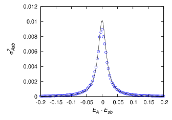
The local density of states, , for the Hubbard model at and is shown in Fig. 17. It fits well to the Lorentzian form (19) with given by (20).
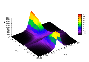
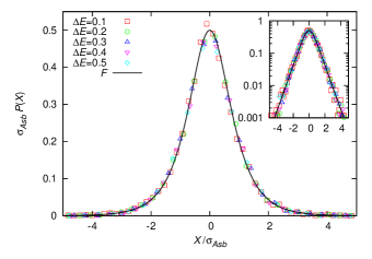
We can also discuss the full distribution of the overlaps . For a system with time reversal symmetry, can be constructed to be real. Our numerical results for a system at and are shown in Fig. 18. This is a histogram using the overlaps of all the eigenstates with a subset of product states where the bath states are within an energy of the centre of the bath spectrum. We can see that the width of the distribution is a strong function of the energy difference between and . The widest distribution is found at . In this case, the states effectively form a random basis for the eigenstates .
The distributions appear to be controlled by a single variable, the local density of states. In other words,
| (21) |
for a normalised distribution with unit variance. This is demonstrated in Fig. 19 for our data at five different . The data have been scaled using the expected width given by (19) and (20). So, this data collapse contains no adjustable parameters. The distribution has an excess kurtosis numerically. ( would be zero for a Normal distribution.) In Fig. 19, we see that our data are well approximated by a hyperbolic secant distribution which has an excess kurtosis of 2:
| (22) |
We should point out that the data collapse to this distribution fails at strong coupling. This may be due to the fact that the width of the distribution becomes large enough that each eigenstate involves bath states in a wide range of energies over which the bath density of states varies significantly.
We note that our form for the overlap distribution differs from what may be expected from random matrix theory Berry (1977); Deutsch (1991); Srednicki (1994) for similar types of overlaps which suggests that they should follow a Normal distribution at weak coupling. This indicates that the overlap distribution may depend details of the coupling Hamiltonian or details of random matrix ensemble.
Accepting the distribution (21) as the distribution for the overlaps, the distribution for the squared overlaps can be derived:
| (23) |
which has a mean of and a variance of . In the case where the overlap distribution is so wide that is effectively a random vector in the basis of , we have a Porter-Thomas distribution for the local density of states.
To summarise, we have shown that our numerics agree with results for the local density of states arising from generic random Hamiltonians. This controls the overlap distribution. We point out that in this simple picture of the statistics of the overlaps, any correlations between different eigenstate overlaps are implicitly neglected. We will now proceed to understand eigenstate thermalisation in terms of this simple picture of eigenstate overlaps .
IV.2 Scaling of Eigenstate Thermalisation with Coupling Strength
In Section III.7, we found that the degree of eigenstate thermalisation improves upon increasing the strength of the subsystem-bath coupling. In the previous section, we have seen (19) that, in parallel, increasing the coupling strength broadens the local density of states. We expect that, as the distribution of overlaps broadens such that more basis states participate in each eigenstate, the fluctuations in the projection values will be reduced in accordance with the law of large numbers. We will show this to be the case and find the -dependence for the spread of eigenstate projections , found numerically in Section III.
From its definition (II.3), the projection operator sums over all bath states. In our model of the overlaps, is a sum over many independent variables. Its mean and variance are given by
| (24) |
For the full distribution of these quantities, see Appendix A which applies the central limit theorem to our model distribution for the overlaps.
First, we consider the mean for a given subsystem state . From our model , this is the sum over all bath states (with the necessary spin and particle number) using a Lorentzian window of energy centered at . In other words, the answer should be proportional to the bath density of states at . Furthermore, we have the normalisation condition . So, at fixed , should give the normalised probability of finding the subsystem in state according to the Gibbs distribution:
| (25) |
where , and are the energy, number and spin of the state , is the density of bath states with energy in an interval about , particles and spin . Thus, we see that a simple model of the eigenstate overlaps gives the canonical thermal distribution Deutsch (1991); Srednicki (1994); Tasaki (1998).
Next we address the spread of the projection values . Using the Lorentzian form (19) for the local density of states with width , and following the same approximations as above, the sum over is:
| (26) |
This means that the spread of the projection values is given by:
| (27) |
where we have used our estimate (20) for the Lorentzian width . Note that is of the order of the average level spacing .
Therefore, we find that is proportional to as shown numerically in Fig. 16. Moreover, we see that so that the fluctuations in the projection values are small for large systems, in accordance with the law of large numbers for a quantity that is a sum over many states.
We stress that the above results hold for any distribution of matrix elements , of sensible form, where the central limit theorem applies. Furthermore, the result (25) holds quite generally for any sensible form of which is a function of with a peak at . Although we have not derived it here explicitly, it should also be noted that the off-diagonal elements of the reduced density matrix, which were found to be virtually zero numerically, are expected to be zero from this model of eigenstate overlaps. Indeed the mean values of the eigenstate expectation-values for off-diagonal elements are clearly zero due to the random sign of eigenstate overlaps.
V Crossover to Thermalisation
In this section, we will try to understand the onset of thermalisation using simple theoretical arguments. In particular, we explore the effects of system size on the thermalisation for the cases of interacting and non-interacting fermions in the Hubbard model. The extent to which the effects of system size on thermalisation may be seen numerically is limited, as discussed in Section III.5. We proceed to identify a minimum coupling strength below which thermalisation cannot occur.
To begin to see thermalisation requires the coupling Hamiltonian to be big enough to mix the eigenstates non-perturbatively. We will then compare this theoretical estimate with our numerical results.
For small coupling strength (), the overlap between an eigenstate and a subsystem-bath product state takes the form
| (28) |
to second order in , where the state is the composite eigenstate to zeroth order in . (Note that has no diagonal elements in this basis.) The threshold for non-perturbative mixing may be considered to be met when the second-order term equals the first order term in magnitude. Note that the bath states coupled by have different quantum numbers from the given state so that there is no level repulsion between and . We expect the nearest bath state is on average away in energy. Generically, this occurs around a coupling strength which we define by
| (29) |
where is the bath level spacing and is the typical magnitude of the square of a coupling matrix element. We will estimate these below for interacting and non-interacting systems.
The quantity should be the coupling strength at which one starts to see a departure from complete memory of the initial state at long times. We therefore expect that this quantity should be similar to the quantity , introduced in Section III, which measures the crossover from the non-thermalised regime to thermalisation. Note that has been defined with an arbitrary choice of a threshold for at 25%. Its actual value will change with the specific criterion chosen to mark this threshold. However, one can use the data from Fig. 11 to show that the relative values for for different system parameters are approximately the same for a range of choice of thresholds. So, it is reasonable to discuss a relationship between and . In particular, it is expected that the two quantities should be proportional to each other for a given subsystem size.
The rest of this section is dedicated to understanding the scaling of with system size. First we will consider the case of finite interactions before, in the subsection following, discussing the case of virtually free fermions where .
V.1 System-Size Scaling for Interacting Fermions

We will now deduce the scaling of with system size for the Hubbard model with interactions . To find the theoretical scaling of with system size requires a knowledge of the scaling of both the energy spacing between coupled states and the scaling of the magnitude of the typical matrix elements with system size. A characteristic submatrix of the coupling matrix , with and fixed, is shown in Fig. 20 for the Hubbard model with interaction strength . The non-zero elements of the coupling matrix form a band. This can be explained by the single-particle nature of the coupling. In the limit of zero interactions, the coupling involves a single particle hopping into, or from, one of the single-particle states in the bath. Therefore, the full width, , for bath states into which a particle may hop is , the single-particle bandwidth. The presence of interactions preserves the banded structure of the coupling matrix and, provided , the banded matrix is not significantly broadened beyond . However, when , the details of single-particle bath states are blurred as the single-particle quasiparticle weight is significantly reduced from unity.
First of all, we estimate the magnitude of a matrix element . To keep the description straightforward, we consider the case of exactly half filling. We will compute this from the average for the sum of all the squared matrix elements . The calculation of this trace can be found in Appendix B. We find:
| (30) |
where is the dimension of the Hilbert space of the composite system. We now need to count the number of non-zero matrix elements in the coupling matrix . Since the coupling involves the hopping of a single particle of a given spin state between the subsystem and bath, any given subsystem state , will only have non-zero matrix elements with at most four other subsystem states , corresponding to changing the particle number or spin by . So, there should be approximately such non-zero blocks in the coupling matrix where is the dimension of the subsystem Hilbert space. Each block has a banded structure similar to the one shown in Fig. 20. Note that the bath states, and , connected by belong to subsectors of the bath spectrum with different quantum numbers. For a band of full width , the banded block should have non-zero elements where is the average bath level spacing and is the total number of bath states in the bath subsector of a given number and spin. So, the total number of non-zero elements in the coupling matrix is approximately . Therefore, the mean squared value of each coupling matrix element, , is
| (31) |
using which is valid for the case in Fig. 20 where as discussed above. So, from (29), we see that non-perturbative mixing occurs when reaches
| (32) |
For the purposes of understanding how this threshold scales with system size, we have approximated the bath level spacing as a simple multiple of the average level spacing of the composite system: .
We have arrived at this condition using simple arguments based on perturbation theory. A similar criterion can be obtained using our results for eigenstate thermalisation. In terms of the eigenstate projection values, the system does not thermalise if the spread of the projection values, , becomes comparable to the mean . We have shown in (25) that the latter gives the canonical state which is of the order of where is the number of states in the subsystem. Thus, from (27), the condition that for a given total energy and a subsystem state becomes the criterion that where
| (33) |
Since is simply the average of over the bath sector, we see that the thresholds and , based on different criteria, describe essentially the same crossover. is larger than as might be expected since the latter marks the loss of memory of the initial state while the latter marks the onset of the canonical thermal state.
It remains to establish how the level spacings depends on the system size. Assuming the cosine dispersion for a tight-binding band and neglecting the broadening due to finite , the many-body bandwidth for sites is at half filling. This is found approximately by finding the maximum and minimum composite energy eigenvalues, , by summing the energies of the highest and lowest single-particle eigenstates. Therefore, the mean level spacing is
| (34) |
At half filling, the Hilbert-space dimension is
| (35) |
Therefore, using (32) and Stirling’s approximation for large , we find that the threshold for the loss of memory of the initial state which allows the onset of thermalisation occurs at
| (36) |
Reassuringly, tends to zero as tends to infinity so that, for baths in the thermodynamic limit, arbitrarily small couplings lead to thermalisation, as we expect Feynman (1998). For a lattice of nine sites we estimate this sets .
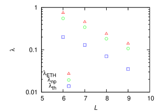
We now compare , for different lattice sizes, with . To allow easy comparison between different system sizes, the composite energy in the centre of the band will be considered in each case. As already discussed, the value of where the value is recorded is somewhat arbitrary. However, we find good agreement between and , as is shown in Fig. 21, with defined using a threshold of . If thresholds other than =25% are considered, we find that changes approximately by a multiplicative constant for all . Therefore, the good agreement between the explicit values for and is not a remarkable feature of Fig. 21. However, that the two quantities are found to scale in virtually the same way for the limited numerical data available provides numerical evidence to support the system-size scaling of thermalisation (36) derived above.
V.2 System-Size Dependence for Non-Interacting Fermions
For the case of almost free fermions (), thermalisation was not seen in the nine-site Hubbard ring. We now repeat the argument above for the case of negligible . The major difference from the case of above is the structure of the coupling matrix. Shown in Fig. 22 is the striped form of the coupling matrix. Without interactions, the bath eigenstates are simply Slater determinants of free-fermion single-particle states. Therefore, for each spin, the coupling Hamiltonian has non-zero matrix elements only at energies corresponding to the single-particle bath states for each spin.

When considering the threshold for non-perturbative mixing, it must now be noted that coupled states differ not by the level spacing , but by the bath single-particle level spacing , where . The magnitude of , as given by (30), is independent of . Therefore, using (32) with replaced by , we see that for should be given by
| (37) |
This yields a value for the nine-site lattice. It is therefore clear why initial-state independence is not seen for the nine-site lattice when : the threshold for non-perturbative coupling occurs at a coupling strength some 20 times bigger than for the Hubbard model with interactions . Eq. (37) indicates that the case needs a lattice with 2700 sites in order that falls to the same value as for the interacting case.
We have argued that thermalisation for small systems occurs at smaller system sizes for the interacting system compared to the non-interacting system. We will now ask how the crossover from the regime to the regime occurs. This should occur when the width of the stripes in the coupling matrix elements seen in Fig. 22 becomes comparable to the single-particle level spacing . The stripe width should be the quasiparticle decay rate due to interparticle collisions. At small , the decay rate can be estimated using Fermi’s golden rule. The matrix elements are proportional to and the density of single-particle states is proportional to . So, for single-particle energies far from the Fermi level so that we can neglect effects from Pauli exclusion, the decay rate should be . This becomes comparable to , when reaches . This estimate give the scale for the interaction strength beyond which we see thermalisation in the numerical results shown in Fig. 12. We have only four system sizes and there is a strong even-odd effect in the system size, making it difficult to verify our prediction quantitatively.
VI Experimental Implications
Models such as the Hubbard model studied in this work can be simulated readily using cold atoms in optical lattices Bloch (2005). Thanks to recent rapid progress in addressing single sites in optical lattices Bakr et al. (2009); Sherson et al. (2010); Weitenberg et al. (2011); Endres et al. (2011), models similar to those we studied here can now in principle be implemented and measured in systems of ultracold atoms trapped in optical lattices. In particular, single-site imaging capability means that atom occupation (albeit up to number modulo two) and the spin species can be determined accurately at a few lattice sites that will form the subsystem. This means the state of the subsystem can be probed directly. Single-site addressability means the subsystem and the bath can be initialised with pure quantum states with well-defined number and spin. Furthermore, instead of focusing the probe laser beam on a single site, the laser can be aimed accurately (to within a tenth of the lattice spacing Weitenberg et al. (2011)) between two neighbouring sites, to tune the lattice potential locally and thus adjust the coupling between the subsystem and bath. Both or regimes can be accessed with a blue- or red-detuned laser focussed between the sites.
We expect our findings to be seen for bath state with a relatively well-defined energy (which overlaps bath eigenstates only within a range of energies much smaller than the many-body bandwidth), far from a strongly-correlated ground state. We should point out that, although we focussed on a specific Hamiltonian with specific initial conditions, we believe that our results are generally applicable. For instance, we obtain similar results for Bose and fermion Hubbard models. Also, although we have used an initial bath state (4) consisting of bath eigenstates within a narrow energy window, our results (Fig. 13) are not sensitive to the width of this energy window. Our results should hold for initial states spanning a larger window of bath energies which would be easier to prepare experimentally. Our results also do not change if we introduce random coefficients in the linear superposition of bath eigenstates or change the shape of the window, consistent with the results of Ref Linden et al. (2009).
Moreover, experimental systems will be larger and contain many more atoms than in our simulation. We have shown that the threshold in the coupling strength is exponentially small in the system size for large systems. So, we believe it would be possible to see thermalisation at smaller in experimental systems, even if the initial bath state is simply a single eigenstate.
We should also ensure that the time needed for thermalisation to be seen should be within the lifetime of an optical lattice experiment, typically hundreds of milliseconds or more. Our previous work Genway et al. (2010) for systems with shows that the relaxation towards equilibrium occurs with a relaxation rate for weak coupling (showing exponential decay) and when (showing Gaussian decay). (See Fig. 4 of Genway et al. (2010).) For current optical lattice experiments with 40K, using an optical lattice laser wavelength of nm, the hopping matrix element is approximately 380 Hz for a laser strength of 5 times the recoil energy (), and Hz for . Hence, expected relaxation time scales when range from about ms at in the Gaussian regime, to about ms at in the exponential regime. (The corresponding time scales for range from ms to ms.) For the other commonly used species 6Li, the lighter mass means shorter time scales than for 40K. For an optical lattice laser wavelength of nm, the corresponding Gaussian relaxation time scale is about ms and ms for exponential regime, with . Hence, for optical lattice laser strengths that are not too large, the relaxation times are well within experimental lifetime of the cold atom systems.
Finally, we point out that it is not necessary to use a ring or one-dimensional geometry (as studied in this paper) to see the thermalisation physics we have presented. As long as the inelastic scattering length is small compared to the size of the bath, we expect the qualitative aspects of thermalisation to survive, although the precise values for the various crossovers and thresholds will change depending on the dimensionality of the bath and the nature of subsystem-bath coupling.
VII Conclusions
We have presented an account of the thermalisation of a local subsystem within a closed quantum system described by a lattice of interacting fermions. The subsystem thermalises in the sense that its reduced density matrix approaches the form expected for a canonical thermal ensemble. This thermalisation occurs over a wide range of system parameters for surprisingly small systems. The equilibrium state depends very little on the strength of subsystem-bath coupling provided it meets the following two conditions. Most importantly, the coupling strength needs to be large enough to mix the eigenstates of the uncoupled system non-perturbatively. Secondly, the coupling strength must not be so large that the boundary effects associated with the coupling dominate the behaviour. We also find that small lattice clusters thermalise for a range of interaction strengths, provided is large enough that the system is away from integrability at . We were also able to demonstrate that the energy width of the initial pure state of the bath has virtually no effect on the subsystem state at long times. This was found for a range of energy widths spanning nearly two orders of magnitude.
Numerically, we demonstrated the relationship between subsystem thermalisation at long times and the eigenstate thermalisation hypothesis. We further quantified the extent to which eigenstate thermalisation holds by measuring the spread of eigenstate expectation values for subsystem occupation probabilities. Using generic results for the eigenvectors of perturbed quantum systems in random matrix theory, we were able to derive theoretically a coupling-strength threshold for thermalisation which is in qualitative agreement with our numerical threshold . This establishes a link between the eigenstates of weakly-coupled bipartite quantum systems and eigenstate thermalisation. As this result employed only random matrix theory, our conclusions should be quite general for non-integrable systems, provided that the system is prepared at an energy far from the ground state where correlations may become important.
We were also able to understand the system-size scaling of the breakdown of thermalisation seen in our numerics for interacting fermions by considering a coupling-strength threshold, , below which non-perturbative mixing of eigenstates does not occur. We demonstrated that this non-perturbative threshold has virtually the form as . Moreover, these have the same system-size scaling as the empirical .
We deduced that these thresholds for thermalisation should tend to zero exponentially in the system size. We also attribute the lack of non-perturbative mixing as the reason for the lack of thermalisation for the weak-interaction limit of the small systems we studied. For very large Hubbard rings, we predict that non-perturbative mixing does occur for any non-zero interaction .
During preparation of this manuscript we became aware of unpublished work by Neuenhahn and Marquardt Neuenhahn and Marquardt (2010) which also studies eigenstate thermalisation using random-matrix-theory results for eigenstate overlaps. The authors study the momentum distribution of interacting fermions on an entire closed system, in contrast to the local observables on bipartite quantum systems considered in this work.
Acknowledgements.
SG acknowledges financial support from EPSRC DTA funding and The Leverhulme Trust under grant no. F/00114/B6. AH acknowledges financial support in the earlier part of the project from an EPSRC Advanced Research Fellowship. We acknowledge insightful discussions with John Chalker, Fabian Essler, Stefan Kuhr and Michael Köhl.Appendix A Overlaps and related distributions
We start with the distribution of overlaps in Eq. (21) with zero mean, variance and fourth moment . Since the projection is given by , we first consider the distribution, for :
| (38) | ||||
which has mean and variance . Then, the eigenstate projection values have the distribution , given by
| (39) |
where is the total number of bath states and, since and are fixed, the notation is abbreviated such that . Since this is a sum of many independent random variables, albeit from different probability distributions, it is reasonable to ask if a central limit exists. Indeed, the Lyapunov condition for a generalised central limit does hold Billingsley (1995). To find this central limit, we adopt the standard procedure of factorising the integrals in Fourier space. Upon taking the Fourier transform
| (40) |
the contributions from each of the bath states factorise such that
| (41) |
where
| (42) |
where the series has been truncated to second order in . The logarithm of takes the form of the series
| (43) |
The coefficient to the term linear in is simply and the coefficient to the term is where and are defined in (24). We have dropped terms of higher order of the form . Using (19) and following the same argument that leads to (26),
| (44) |
where is the density of states at and is the reduced density matrix for the canonical thermal state (6). Therefore, we see that the truncation of the series is reasonable for .
Upon re-exponentiating the series, we see the bulk of the distribution may be described accurately with up to the scale of , since the central limit only breaks down at . (This condition is readily met in our numerics when the coupling strength is large enough for the subsystem to approach thermalisation.) Exponentiating and inverting the Fourier transform yields the distribution for eigenstate expectation-values:
| (45) |
which is a Normal distribution with mean and variance .
Appendix B Coupling matrix
In this section, we estimate the magnitude of a matrix element of the coupling matrix as defined in (3). As discussed in Section V, the coupling matrix involves only single-particle hopping between the subsystem and the bath. So, it should connect states not further apart in energy than the single-particle bandwidth .
We will consider the coupling matrix to be a banded matrix where the non-zero elements form a band of full width . While enumerating the size of individual matrix elements is not possible without full diagonalisation of the Hamiltonian, the quantity is basis-independent and may be found readily in the Fock basis, with states , where particles are localised. In this case: .
The matrix does not change the total particle number. To keep the description straightforward, we consider the case of exactly half filling. This is demonstrated in Fig. 23. For each basis state , there are at most only four other basis states which are related by hopping a single fermion (spin up or down) between the subsystem and the bath via either one of the two subsystem-bath links. As the lattice is taken to be exactly half-filled, for each spin and for each topological link between subsystem and bath, half of the Fock states have a filled site adjacent to an empty site across each coupling link. This diagram shows four possible occupations of two sites (across the coupling link at =2 and 3) by spin-up fermions, irrespective of the configuration of spin-down fermions on these sites. At half filling, the full -site Fock states may be divided up into four groups containing equal numbers of states, with each group having the spin-up occupations A, B, C and D (as labelled in the figure). Each state in groups A and B can couple to one other Fock state, with matrix element , but states in groups C and D couple to no other Fock states. Spin-down fermions do not affect these matrix elements.
Therefore, each spin and each subsystem-bath link contributes to the trace where is the dimension of the Hilbert space of the composite system. There are contributions from two links and two spin species. Hence, we obtain
| (46) |
References
- Cazalilla and Rigol (2010) M. A. Cazalilla and M. Rigol, New Journal of Physics 12, 055006 (2010).
- Polkovnikov et al. (2011) A. Polkovnikov, K. Sengupta, A. Silva, and M. Vengalattore, Rev. Mod. Phys. 83, 863 (2011).
- Yukalov (2011) V. I. Yukalov, Laser Phys. Lett. 8, 485 (2011).
- Gemmer et al. (2005) J. Gemmer, M. Michel, and G. Mahler, Quantum Thermodynamics: Emergence of Thermodynamic Behavior Within Composite Quantum Systems, Lecture Notes in Physics (Springer, 2005).
- Saito et al. (1996) K. Saito, S. Takesue, and S. Miyashita, Journal of the Physical Society of Japan 65, 1243 (1996).
- Yuan et al. (2009) S. Yuan, M. I. Katsnelson, and H. De Raedt, Journal of the Physical Society of Japan 78, 094003 (2009).
- Jin et al. (2010) F. Jin, H. De Raedt, S. Yuan, M. I. Katsnelson, S. Miyashita, and K. Michielsen, Journal of the Physical Society of Japan 79, 124005 (2010).
- Henrich et al. (2005) M. Henrich, M. Michel, M. Hartmann, G. Mahler, and J. Gemmer, Physical Review E 72, 026104 (2005).
- Gogolin et al. (2011) C. Gogolin, M. Müller, and J. Eisert, Physical Review Letters 106, 040401 (2011).
- Cho and Kim (2010) J. Cho and M. S. Kim, Physical Review Letters 104, 170402 (2010).
- Tasaki (1998) H. Tasaki, Physical Review Letters , 1373 (1998).
- Goldstein et al. (2006) S. Goldstein, J. Lebowitz, R. Tumulka, and N. Zanghì, Physical Review Letters 96, 050403 (2006).
- Popescu et al. (2006) S. Popescu, A. J. Short, and A. Winter, Nature Physics 2, 754 (2006).
- Reimann (2007) P. Reimann, Physical Review Letters 99, 160404 (2007).
- Reimann (2008) P. Reimann, Physical Review Letters 101, 190403 (2008).
- Linden et al. (2009) N. Linden, S. Popescu, A. Short, and A. Winter, Physical Review E 79, 061103 (2009).
- Gogolin (2010) C. Gogolin, Physical Review E 81, 051127 (2010).
- Lychkovskiy (2010) O. Lychkovskiy, Physical Review E 82, 011123 (2010).
- Deutsch (1991) J. M. Deutsch, Physical Review A 43, 2046 (1991).
- Srednicki (1994) M. Srednicki, Physical Review E 50, 888 (1994).
- Rigol et al. (2008) M. Rigol, V. Dunjko, and M. Olshanii, Nature 452, 854 (2008).
- Sherson et al. (2010) J. F. Sherson, C. Weitenberg, M. Endres, M. Cheneau, I. Bloch, and S. Kuhr, Nature 467, 68 (2010).
- Bakr et al. (2010) W. S. Bakr, A. Peng, M. E. Tai, R. Ma, J. Simon, J. I. Gillen, S. Fölling, L. Pollet, and M. Greiner, Science 329, 547 (2010).
- Rigol et al. (2007) M. Rigol, V. Dunjko, V. Yurovsky, and M. Olshanii, Physical Review Letters 98, 050405 (2007).
- Berry (1977) M. V. Berry, Journal of Physics A: Mathematical and General 10, 2083 (1977).
- Rigol and Santos (2010) M. Rigol and L. Santos, Physical Review A 82, 011604 (2010).
- Ji and Fine (2011) K. Ji and B. Fine, Physical Review Letters 107, 050401 (2011).
- Fine (2009) B. V. Fine, Physical Review E 80, 051130 (2009).
- Canovi et al. (2011) E. Canovi, D. Rossini, R. Fazio, G. E. Santoro, and A. Silva, Phys. Rev. B 83, 094431 (2011).
- Lesanovsky et al. (2010) I. Lesanovsky, B. Olmos, and J. Garrahan, Physical Review Letters 105, 100603 (2010).
- Ates et al. (2012) C. Ates, J. Garrahan, and I. Lesanovsky, Physical Review Letters 108, 110603 (2012).
- Kinoshita et al. (2006) T. Kinoshita, T. Wenger, and D. S. Weiss, Nature 440, 900 (2006).
- Eckstein and Kollar (2008) M. Eckstein and M. Kollar, Phys. Rev. Lett. 100, 120404 (2008).
- Sotiriadis et al. (2009) S. Sotiriadis, P. Calabrese, and J. Cardy, EPL (Europhysics Letters) 87, 20002 (2009).
- Calabrese et al. (2011) P. Calabrese, F. H. L. Essler, and M. Fagotti, Phys. Rev. Lett. 106, 227203 (2011).
- Cassidy et al. (2011) A. Cassidy, C. Clark, and M. Rigol, Physical Review Letters 106, 140405 (2011).
- Poilblanc (2011) D. Poilblanc, Phys. Rev. B 84, 045120 (2011).
- Jensen and Shankar (1985) R. Jensen and R. Shankar, Physical Review Letters 54, 1879 (1985).
- Eckstein et al. (2009) M. Eckstein, M. Kollar, and P. Werner, Phys. Rev. Lett. 103, 056403 (2009).
- Genway et al. (2010) S. Genway, A. Ho, and D. K. K. Lee, Physical Review Letters 105, 260402 (2010).
- Kollar et al. (2011) M. Kollar, F. A. Wolf, and M. Eckstein, Phys. Rev. B 84, 054304 (2011), arXiv:1102.2117 [cond-mat.str-el] .
- Kottos and Cohen (2001) T. Kottos and D. Cohen, Physical Review E 64, 065202 (2001).
- Cohen et al. (2000) D. Cohen, F. M. Izrailev, and T. Kottos, Physical review letters 84, 2052 (2000).
- Hiller et al. (2006) M. Hiller, T. Kottos, and T. Geisel, Physical Review A 73, 061604 (2006).
- Wigner (1955) E. P. Wigner, Annals of Mathematics 62, 548 (1955).
- Wigner (1957) E. P. Wigner, Annals of Mathematics 67, 325 (1957).
- Note (1) In preparation.
- Feynman (1998) R. Feynman, Statistical mechanics: a set of lectures, Advanced book classics (Westview Press, 1998).
- Bloch (2005) I. Bloch, Nature Physics 1, 23 (2005).
- Bakr et al. (2009) W. S. Bakr, J. I. Gillen, A. Peng, S. Fölling, and M. Greiner, Nature 462, 74 (2009).
- Weitenberg et al. (2011) C. Weitenberg, M. Endres, J. F. Sherson, M. Cheneau, P. Schauß, T. Fukuhara, I. Bloch, and S. Kuhr, Nature 471, 319 (2011).
- Endres et al. (2011) M. Endres, M. Cheneau, T. Fukuhara, C. Weitenberg, P. Schauß, C. Gross, L. Mazza, M. C. Bañuls, L. Pollet, I. Bloch, and S. Kuhr, Science 334, 200 (2011).
- Neuenhahn and Marquardt (2010) C. Neuenhahn and F. Marquardt, ArXiv e-prints (2010), arXiv:1007.5306 [cond-mat.stat-mech] .
- Billingsley (1995) P. Billingsley, Probability and Measure (Wiley, 1995).