Extremal spacings between eigenphases of random unitary matrices
and their tensor products

Abstract

Extremal spacings between eigenphases of random unitary matrices of size $N$ pertaining to circular ensembles are investigated. Explicit probability distributions for the minimal spacing for various ensembles are derived for $N=4$. We study ensembles of tensor product of $k$ random unitary matrices of size $n$ which describe independent evolution of a composite quantum system consisting of $k$ subsystems. In the asymptotic case, as the total dimension $N=n^{k}$ becomes large, the nearest neighbor distribution $P(s)$ becomes Poissonian, but statistics of extreme spacings $P(s_{\rm min})$ and $P(s_{\rm max})$ reveal certain deviations from the Poissonian behavior.

I Introduction

Random unitary matrices are useful to describe spectra of periodic quantum systems, the classical analogues of which are chaotic H06 ; S99 . The choice of a specific ensemble of matrices is dictated by symmetry properties of the investigated physical system. If the system possesses no time-reversal symmetry the circular unitary ensemble ($\operatorname{CUE}$) of matrices distributed according to the Haar measure of the unitary group is appropriate  Me04 . For systems with a generalized time reversal symmetry the circular orthogonal ensemble ($\operatorname{COE}$) describes properly statistical properties of spectra if we neglect additional subtleties caused by specific rotational symmetry features of systems with half-integer spin, which are of no concern for investigations reported in this paper. In the case of classically regular dynamics the spectrum of the evolution operator displays level clustering characteristic to the circular Poissonian ensemble ($\operatorname{CPE}$) of diagonal random unitary matrices. To describe intermediate statistics one uses interpolating ensembles of unitary matrices PS91 ; LZ92 ; ZK96 or composed ensembles of unitary matrices Poz . In the case of emerging chaos, in which the chaotic layer covers only a fraction of the phase space of the classical system one may apply the distribution of Berry and Robnik, originally used for autonomous systems BR84 .

To characterize statistical properties of spectra of a random matrix one often uses the nearest neighbor spacings distribution $P(s)$ Me04 ; Fo10 . The random variable $s$ is the distance between adjacent eigenphases (phases of eigenvalues) normalized by assuming that the mean spacing is equal to unity.

In this work we investigate the distribution of yet another random variable – the minimal spacing $s_{\rm min}$ between two eigenphases. In similarity to the standard statistics of nearest level spacings, also the distribution $P(s_{\min})$ encodes information about properties of the spectrum. Observe that for any unitary matrix $U$ the size of its minimal spacing $s_{\rm min}$ provides an information, to which extent the investigated matrix $U$ is close to be degenerated. For completeness we are also going to study the size of the largest spacing $s_{\rm max}$ defined analogously.

Statistics of the minimal spacings in spectra of random Hermitian matrices was analyzed by Caër et al. CMD07 and also discussed in the book by Forrester Fo10 . Our current approach is somewhat similar but different, as we investigate extremal gaps between eigenvalues of unitary matrices distributed along the unit circle and study tensor products of unitary matrices. After a part of our project was completed we learned about a relevant work of Arous and Bourgade AB10 in which the distribution of extremal spacings was studied for random matrices of circular unitary ensemble.

The paper is organized as follows. For exemplary ensembles of random matrices of size $N=4$ we derive in Section II exact forms of the distributions of minimal spacings. The chosen dimension allows exact calculations, which become rather complicated for larger matrices. Moreover, this is the minimal dimension in which results for $\operatorname{CUE}$ and $\operatorname{CPE}$ can be compared with those for the ensemble consisting of tensor products of two $\operatorname{CUE}$ random matrices of size $N=2$. Such an ensemble corresponds to a generic local dynamics in a two-qubit system TSKZZ12 .

The case of large matrices is studied in Section III. We recall the heuristic argument put forward e.g. in Fo10 (see Exercise 14.6.5, p. 697) justifying that for a random unitary matrix of size $N$ the size of the minimal gap scales as $s_{\min}\approx N^{-\frac{1}{1+\beta}}$ where $\beta=0,1$ and $2$ for the Poissonian, orthogonal and unitary circular ensemble, respectively. Analogously, we approach the asymptotic scaling of the maximal gap $s_{\max}$. We also provide some numerical results confirming our non-rigorous predictions concerning the order of the mean values of the extremal spacings $\langle s_{\min}\rangle$, $\langle s_{\max}\rangle$, and the distribution of the minimal spacing $s_{\min}$. Recently, the latter has been rigourously studied in AB10 and Sh07 . It was considered for the first time in Vi01 .

Furthermore, we analyze extremal spacings for products of $k$ independent random unitary matrices, each of them of size $n$. If the total dimension of the matrix, $N=n^{k}$, is large the level spacing distribution $P(s)$ becomes Poissonian TSKZZ12 . This property holds also for a tensor product of two random unitary matrices of a different size Tk13 . However, in the case of a large number of one-qubit systems, ($n=2$ and $k$ large), statistics of the minimal spacing $s_{\rm min}$ displays significant deviations from the predictions for the Poisson ensemble, reviewed in the Appendix.

We use the following notation. For a single unitary or orthogonal matrix $A$ of size $N$ we consider its spectrum $\{\exp(i\varphi_{j})\}_{j=1}^{N}$, where $(\varphi_{1},\ldots,\varphi_{N})$ represents the vector of the eigenphases ordered non-decreasingly, $0\leq\varphi_{1}\leq\ldots\leq\varphi_{N}<2\pi$. We order non-decreasingly the spacings $\varphi_{2}-\varphi_{1},\ldots,\varphi_{N}-\varphi_{N-1},2\pi+\varphi_{1}-\varphi_{N}$ between neighboring eigenphases, divide them by the average spacing $2\pi/N$ and denote the obtained sequence by

$$s_{\rm min}:=s_{1}\leq\ldots\leq s_{N}=:s_{\rm max}.$$ (1)

The standard level spacing distribution $P(s)$ is given by the average $\frac{1}{N}\sum_{m=1}^{N}P_{m}(s_{m})$, where $P_{m}$ is the density of the rescaled $m$-th spacing $s_{m}=(\varphi_{m+1}-\varphi_{m})N/2\pi$.

II Case study: minimal spacings for two–qubit system

Our first goal is to derive exact probability distributions of the minimal spacing $P_{\min}$ for exemplary ensembles of random unitary matrices of size $N=4$. Besides the Poissonian and the unitary ensemble we analyze also the tensor product of two independent random matrices of size $N=2$. This ensemble, denoted for brevity as CU$E_{2\otimes 2}$, describes dynamics of two independent quantum sub-systems TSKZZ12 . In the quantum information literature such a case is called a two–qubit system.

To derive the desired distribution we calculate the tail distribution $T(t)=\mathbb{P}\left(s_{\min}>t\right)$ and take the derivative of $T$. We have

$$\begin{split}T(t)&=\mathbb{P}\left(s_{\min}>t\right)\\ &=\mathbb{P}\left(\varphi_{2}-\varphi_{1},\varphi_{3}-\varphi_{2},\varphi_{4}-\varphi_{3},2\pi+\varphi_{1}-\varphi_{4}>\pi t/2\right)\\ &=\int_{\{\varphi_{2}-\varphi_{1},\varphi_{3}-\varphi_{2},\varphi_{4}-\varphi_{3},2\pi+\varphi_{1}-\varphi_{4}>\pi t/2\}}\\ &P^{\textrm{ord}}\left(\varphi_{1},\varphi_{2},\varphi_{3},\varphi_{4}\right)d\left(\varphi_{1},\varphi_{2},\varphi_{3},\varphi_{4}\right),\end{split}$$ (2)

where $P^{\textrm{ord}}$ is the joint probability distribution of ordered eigenphases, which can be obtained from the joint probability distribution for a given ensemble. After changing variables, $\psi_{1}=\varphi_{1},\psi_{2}=\varphi_{2}-\varphi_{1},\psi_{3}=\varphi_{3}-\varphi_{2}$ and $\psi_{4}=\varphi_{4}-\varphi_{3}$, the integration domain splits into two tetrahedrons. Standard but tedious calculations yield in each case the tail distribution function $T(t)$, which leads to the corresponding probability density, $P(s_{\min})=-\frac{\mathrm{d}}{\mathrm{d}t}T(t)|_{t=s_{\min}}$.

1. for $\operatorname{CUE}_{2\otimes 2}$,

   $$\begin{split}P^{U}_{2\otimes 2}(s_{\min})=\frac{1}{4\pi}\Big{(}&2\pi(1-s_{\min})\big{(}4-\cos(\pi s_{\min}/2)\big{)}\\ &-3\sin(\pi s_{\min}/2)+8\sin(\pi s_{\min})\\ &-3\sin(3\pi s_{\min}/2)\Big{)},\end{split}$$ (3)

2. for $\operatorname{CUE}_{4}$

   $$\begin{split}P^{U}_{4}(s_{\min})=&\frac{1}{72\pi^{2}}\sin^{2}(\pi s_{\min}/4)\bigg{(}666+720\pi^{2}(1-s_{\min})^{2}\\ &+36\big{(}11+16\pi^{2}(1-s_{\min})^{2}\big{)}\cos(\pi s_{\min}/2)\\ &+18\big{(}8\pi^{2}(1-s_{\min})^{2}-13\big{)}\cos(\pi s_{\min})\\ &-100\cos(3\pi s_{\min}/2)-608\cos(2\pi s_{\min})\\ &-380\cos(5\pi s_{\min}/2)+234\cos(3\pi s_{\min})\\ &+74\cos(7\pi s_{\min}/2)-58\cos(4\pi s_{\min})\\ &+10\cos(9\pi s_{\min}/2)\\ &+24\pi(1-s_{\min})\Big{[}60\sin(\pi s_{\min}/2)\\ &+63\sin(\pi s_{\min})+22\sin(3\pi s_{\min}/2)\\ &+2\sin(2\pi s_{\min})-4\sin(5\pi s_{\min}/2)\Big{]}\bigg{)},\end{split}$$ (4)

3. for $\operatorname{CPE}_{4}$

   $$P^{P}_{4}(s_{\min})=3(1-s_{\min})^{2}.$$ (5)

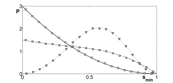
Figure 1: Probability densities of the minimal spacing $s_{\min}$ for random matrices of size $N=4$ pertaining to $\operatorname{CUE}_{4}$ ($\triangledown$), $\operatorname{CUE}_{2\otimes 2}$ ($\square$), and $\operatorname{CPE}_{4}$ ($\circ$). Symbols denote numerical results obtained for $2^{14}$ independent matrices, while the curves represent distributions (3), (4) and (5), respectively.

These three distributions are presented in Fig. 1. The behavior of the densities around zero encodes some information concerning level repulsion and level clustering. The variable $s_{\min}$ is the smallest distance between two neighboring eigenphases. Therefore, the fact that its density is separated from zero, say $P(s_{min})>1$ for $s_{min}$ close to zero, means that for a small $\epsilon>0$ the probability that some two phases are at the distance closer than $\epsilon$ equals $\mathbb{P}\left(s_{\min}<\epsilon\right)=\int_{0}^{\epsilon}P(s_{min})\mathrm{d}s>\epsilon$. In the cases of $\operatorname{CPE}_{4}$ and $\operatorname{CUE}_{4}$ these features are consistent with level clustering and level repulsion observed in the distribution of spacings $P(s)$. Fig. 1 shows that the eigenphases of the tensor product $\operatorname{CUE}_{2\otimes 2}$ tend to accumulate in a spectacular contrast to the case of a single random unitary matrix form $\operatorname{CUE}$ TSKZZ12 .

Numerical results show that for large $N$ the distributions of the $m$–th spacing $P(s_{m})$ are close to the level spacing distribution $P(s)$ for $m\approx N/2$. However, for any $N$ the distributions of the smallest spacing $s_{\min}=s_{1}$ and of the largest spacing $s_{\max}=s_{N}$ differ considerably. We shall then analyze these distributions of extremal spacings, which can be used as auxiliary statistical tools to characterize ensembles of random matrices.

III Extremal statistics for large matrices

In this section we analyze extremal gaps in the spectra of circular ensembles of random matrices of a large size, $N\gg 1$, giving the numerical evidence to support some simple heuristic arguments (the subject for $\operatorname{CUE}$ ensemble has been rigorously studied though, see e.g. AB10 ). As usual, we parameterize canonical ensembles by the level repulsion parameter $\beta$, equal to $0,1$ and $2$ for Poissonian, orthogonal and unitary ensembles respectively. The relevant quantities are labeled by the index $\beta=0,1,2$. For instance $P_{\beta}(s)$ represents the level spacing distribution for the corresponding ensemble of random unitary matrices. We shall start with the Poissonian ensemble described by the case $\beta=0$. Some basic properties of the Poissonian process are reviewed in the Appendix A.

III.1 Asymptotics of the extreme spacings for Poisson process

We are interested in asymptotic properties of spectra of diagonal random unitary matrices. We choose at random $N$ points from the unit circle $\{z\in\mathbb{C},|z|=1\}$, each independently according to the uniform distribution. The arguments of these points ordered non-decreasingly will be called $0\leq\theta_{1}\leq\ldots\leq\theta_{N}<2\pi$. We define a point process $\Xi_{N}$ of the rescaled eigenphases of a diagonal random unitary matrix $D_{N}=\textrm{diag }(e^{i\theta_{1}},\ldots,e^{i\theta_{N}})$ pertaining to CPE_N,

$$\Xi_{N}=\{(N/2\pi)\theta_{1},\ldots,(N/2\pi)\theta_{N}\}.$$ (6)

Moreover, we define the spacings $s_{i}$, $s_{\min}$, and $s_{\max}$ according to (1). Note that the scaling is chosen so that the mean spacing $\langle s\rangle$ is fixed to unity.

For the standard Poisson process $\Pi=\{X_{1},X_{2},\ldots\}$ (see Appendix A), where its points are labeled in the nondecreasing order $0\leq X_{1}\leq X_{2}\leq\ldots$, we also define the spacings

$$Y_{1}=X_{1},\ Y_{2}=X_{2}-X_{1},\ Y_{3}=X_{3}-X_{2},\ \ldots.$$ (7)

It is known that for large $N$ the process $\Xi_{N}$ becomes Poissonian, as the correlation functions converge to the constant functions equal to unity characteristic of the Poisson process $\Pi$.

We would like to address the question of the asymptotic behavior of the variables $s_{\min}$ and $s_{\max}$. Since for a diagonal unitary matrix of CPE the process (6) becomes Poissonian, the variables $\min_{j\leq N}Y_{j}$ and $\max_{j\leq N}Y_{j}$ satisfy

$$\begin{split}\sup_{t\in\mathbb{R}}\left|\mathbb{P}\left(s_{\min}\leq t\right)-\mathbb{P}\left(\min_{j\leq N}Y_{j}\leq t\right)\right|&\xrightarrow[N\to\infty]{}0,\\ \sup_{t\in\mathbb{R}}\left|\mathbb{P}\left(s_{\max}\leq t\right)-\mathbb{P}\left(\max_{j\leq N}Y_{j}\leq t\right)\right|&\xrightarrow[N\to\infty]{}0.\end{split}$$ (8)

In view of (8) we arrive at the desired conclusions regarding $s_{\min}$ and $s_{\max}$. These quantities are of order

$${\langle s_{\min}\rangle}_{\operatorname{CPE}}\sim 1/N,\quad{\langle s_{\max}\rangle}_{\operatorname{CPE}}\sim\ln N.$$ (9)

After rescaling $s_{\min}$ converges to a random variable $y$ with exponential density,

$$Ns_{\min}\overset{d}{\longrightarrow}e^{-y}\textbf{1}_{\{y>0\}},$$ (10)

where by $\textbf{1}_{Y}$ we denote the characteristic function of the set $Y$. The maximal spacing $s_{\max}$ converges to a constant,

$$s_{\max}/\ln N\overset{d}{\longrightarrow}1,$$ (11)

where $\overset{d}{\longrightarrow}$ denotes the convergence in distribution.

The fluctuations of the rescaled variable $s_{\max}/\ln N$ around $1$ are of order $1/\ln N$ and they are described by the Gumbel distribution,

$$s_{\max}-\langle s_{\max}\rangle\overset{d}{\longrightarrow}P(x)\sim e^{-(x+\gamma)-e^{-(x+\gamma)}}.$$ (12)

Here and throughout, we denote by $\gamma\approx 0.5772$ Euler’s constant.

III.2 Mean minimal spacing

For the sake of convenience, we recall here the heurisitic reasoning leading to the estimate of mean of the minimal gap (Exercise 14.6.5 in Fo10 ). In the next subsection we follow this idea to deal with the maximal gap.

To get an estimation of the behavior of the mean minimal spacing of a random unitary matrix of size $N$ let us assume that spacings $s_{j}$, $j=1,\dots,N$ are independent random variables. For small spacing one has $P_{\beta}(s)\sim s^{\beta}$, so the integrated distribution $I_{\beta}(s)=\int_{0}^{s}P_{\beta}(s^{\prime})ds^{\prime}$ behaves as $I_{\beta}(s)\sim s^{1+\beta}$. A matrix $U$ of size $N$ yields $N$ spacings $s_{j}$. Thus the minimal spacing $s_{\min}$ occurs on average for such an argument of the integrated distribution that $I_{\beta}(s_{\min})\approx 1/N$. This implies that $(s_{\min})^{1+\beta}\approx 1/N,$ which allows us to estimate the average minimal spacing

$$\langle s_{\min}\rangle\approx N^{-\frac{1}{1+\beta}}.$$ (13)

In the case $\beta=2$ corresponding to $\operatorname{CUE}$ this statement is consistent with the rigorous results AB10 of Arous and Bourgade. As shown in Fig. 2 the above heuristic reasoning provides the correct value of the exponent in dependence of the mean minimal spacing $\langle s_{\min}\rangle$ on the matrix size $N$ for $\operatorname{CPE}$ $(\beta=0)$, $\operatorname{COE}$ $(\beta=1)$ and $\operatorname{CUE}$ $(\beta=2)$.

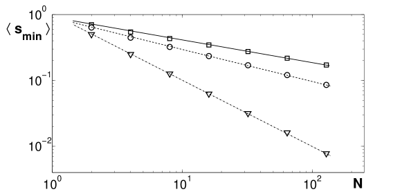
Figure 2: Mean minimal spacing $\langle s_{\min}\rangle$ as a function of the matrix size $N=2^{m}$ for ($\triangledown$) $\operatorname{CPE}$, ($\square$) $\operatorname{COE}$ and ($\circ$) $\operatorname{CUE}$ and $m=1,...,7$. Symbols denote numerical results obtained for $2^{14}$ independent random matrices. Solid, dashed and dash-dot lines are plotted with slopes implied by the estimation (13) and equal to $-1$, $-1/2$ and $-1/3$, respectively. Linear fit to numerical data yields slopes -0.98, -0.48, -0.33, respectively.

III.3 Mean maximal spacing

We study the average maximal spacing $\langle s_{\max}\rangle$ for random unitary matrices of the circular orthogonal ensemble. Matrix of size $N$ yields $N$ spacings $s_{j}$. In analogy to the previous reasoning we shall assume that all spacings are independent random variables described by the Wigner surmise

$$P(s)=\frac{\pi}{2}se^{-\pi s^{2}/4}.$$ (14)

Thus the integrated distribution $I(s)=\int_{0}^{s}P(s^{\prime})ds^{\prime}$ reads $I(s)=1-e^{-\pi s^{2}/4}$. The maximal spacing $s_{\max}$ occurs on average for such an argument of the integrated distribution function that $1-I(s_{\max})\approx 1/N.$ This implies that $e^{-\pi s_{\max}^{2}/4}\approx 1/N$, which allows us to estimate the average maximal spacing,

$$\langle s_{\max}\rangle^{2}_{COE}\approx\frac{4}{\pi}\ln N.$$ (15)

This implies that $\langle s_{\max}\rangle^{2}$ grows with the matrix size N proportionally to $\frac{4}{\pi}\ln N$ what is demonstrated in Fig. (3).

Let us deal now with the circular unitary ensemble. We employ here the Wigner formula for the level spacing distribution of a large $\operatorname{CUE}$ matrix, $P_{2}(s)=\frac{32}{\pi^{2}}s^{2}e^{-4s^{2}/\pi}$. By the same reasoning as above we obtain an estimate that the maximal spacing $s_{\max}$ occurs on average for such an argument of the integrated distribution function $I(s)=\int_{0}^{s}P(s^{\prime})ds^{\prime}$ that $1-I(s_{\max})\approx 1/N$. Thus

$$\frac{1}{N}\approx\int_{s_{\max}}^{\infty}\frac{32}{\pi^{2}}s^{2}e^{-4s^{2}/\pi}\mathrm{d}s.$$ (16)

We change the variable setting $u=4s^{2}/\pi$ and obtain $\frac{1}{N}\approx\int_{4s_{\max}^{2}/\pi}^{\infty}\frac{2}{\sqrt{\pi}}u^{1/2}e^{-u}\mathrm{d}u.$ Therefore, supposing $s_{\max}$ is large we get

$$\frac{1}{N}\approx\frac{4}{\pi}s_{\max}e^{-4s_{\max}^{2}/\pi}.$$ (17)

Now we take the logarithm of both sides, neglect $\ln s_{\max}$ as it is of lower order than $s_{\max}^{2}$ for large $s_{\max}$, and arrive at

$$\langle s_{\max}\rangle^{2}_{CUE}\approx\frac{\pi}{4}\ln N.$$ (18)

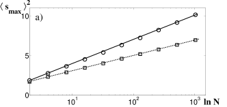
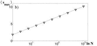
Figure 3: Mean maximal spacing $\langle s_{\max}\rangle$ as a function of the matrix size $N=2^{k}$ with $k=1,...,10$ plotted for a) $\operatorname{CUE}$ ($\circ$), $\beta=2$; $\operatorname{COE}$ ($\square$), $\beta=1$; and b) $\operatorname{CPE}$ ($\triangledown$), $\beta=0$. Symbols denote numerical results obtained for $2^{14}$ independent random matrices. Solid, dashed (panel a) and dash-dot (panel b) lines are plotted with slopes implied by estimations (15), (18) and (19), respectively.

In the case of a Poissonian spectrum the level spacing distribution displays an exponential tail, $P(s)\sim e^{-s}$. Thus the integrated distribution function $I(s)=\int_{0}^{s}P(s^{\prime})ds^{\prime}$ behaves as $I(s)=1-e^{-s}$. For a matrix of size $N$ the maximal spacing $s_{\max}$ occurs on average for such an argument that $1-I(s_{\max})\approx 1/N$. This implies that $e^{-s_{\max}}\approx 1/N$ and enables us to estimate the average maximal spacing for the circular Poisson ensemble as

$$\langle s_{\max}\rangle_{CPE}\approx\ln N.$$ (19)

Analyzing estimations following from eqn. (15), (18) and (19) one obtains slopes $A_{COE}=\frac{4}{\pi}\approx 1.27$, $A_{CUE}=\frac{\pi}{4}\approx 0.77$ and $A_{CPE}=1$, which are comparable with numerical results $A_{COE}\approx 1.33$, $A_{CUE}\approx 0.84$ and $A_{CPE}\approx 0.97$, presented in Fig. 3.

III.4 Distribution of extremal spacings

To study the distributions of the minimal spacing $s_{\rm min}$ we introduce a rescaled variable suggested by (13),

$$x^{(\beta)}_{\min}:=A_{(\beta)}N^{\frac{1}{1+\beta}}s_{\min},$$ (20)

where $A_{(\beta)}$ is a constant, in general different for $\operatorname{CPE}$, $\operatorname{COE}$ and $\operatorname{CUE}$.

The case of the unitary ensemble was recently studied by Arous and Bourgade AB10 , who derived the following expression for the asymptotic distribution of the minimal spacing,

$$P(x_{\min})=3x_{\min}^{2}e^{-x_{\min}^{3}},$$ (21)

in the rescaled variable $x_{\min}=(\pi/3)^{2/3}N^{1/3}s_{\min}$. This result suggests the following general form of the distribution of minimal spacing for all three ensembles considered labeled by the level repulsion parameter $\beta$,

$$P^{(\beta)}(x_{\min}):=(\beta+1)x^{\beta}_{\min}e^{-x^{\beta+1}_{\min}},$$ (22)

which agrees with the numerical data – see Fig. 4.

The above formula has a structure $F(x):=\frac{df(x)}{dx}e^{-f(x)}$, which helps to determine the normalization. Numerical results suggest that constants read: $A_{(0)}=1$ for $\operatorname{CPE}$, $A_{(1)}=\langle s\rangle$ for $\operatorname{COE}$, and $A_{(2)}=(\pi/3)^{2/3}$ for $\operatorname{CUE}$.

Returning to the original variable $s_{\min}$ we obtain the distributions $P^{(\beta)}(s_{\min})$,

$$P^{(0)}(s_{\min})=A_{(0)}Ne^{-Ns_{\min}},$$ (23)

$$P^{(1)}(s_{\min})=2A_{(1)}^{2}Ns_{\min}e^{-A_{(1)}^{2}Ns_{\min}^{2}},$$ (24)

$$P^{(2)}(s_{\min})=3A_{(2)}^{3}Ns_{\min}^{2}e^{-A_{(2)}^{3}Ns_{\min}^{3}}.$$ (25)

The distributions of the minimal spacing obtained numerically for Poisson, orthogonal and unitary circular ensembles of random matrices of the size $N=100$ are presented in Fig. 4.

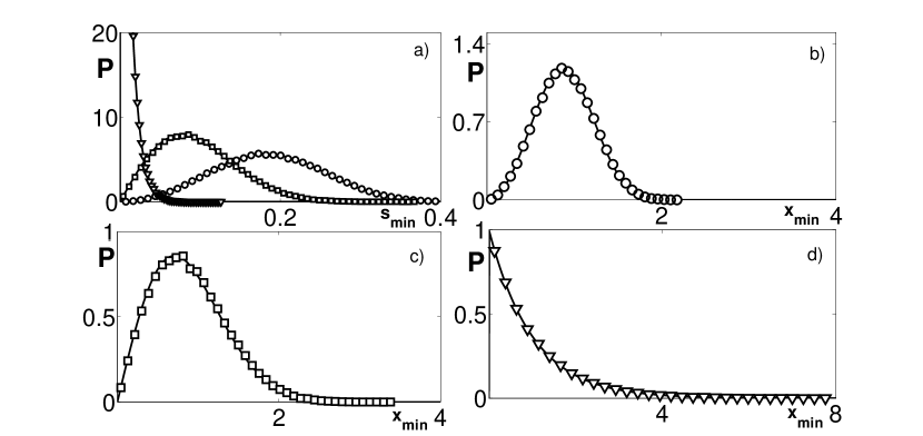
Figure 4: Probability distributions a) $P(s_{min})$ for random unitary matrices of $\operatorname{CUE}$ ($\triangledown$), $\beta=2$; $\operatorname{COE}$ ($\square$), $\beta=1$; and $\operatorname{CPE}$ ($\circ$), $\beta=0$. The same data shown for variable $x_{\rm min}$ rescaled according to (20) for b) $\operatorname{CUE}$, c) $\operatorname{COE}$ and d) $\operatorname{CPE}$. Symbols denote numerical results obtained for $2^{17}$ independent matrices of size $N=100$, while solid curves represent asymptotic predictions (22).

IV Extremal spacings for tensor products of random unitary matrices

In this section we study eigenphases of tensor products of random unitary matrices. We are interested in two cases

1. Two–qunit system: Given two independent $\operatorname{CUE}$ matrices $U_{A},U_{B}$ of size $n$ with eigenphases $\{\psi_{j}\}_{j=1}^{n}$, $\{\phi_{j}\}_{j=1}^{n}$ respectively, define the point process $\Xi_{n}$ of the rescaled eigenphases of the tensor product $U_{A}\otimes U_{B}$

   $$\Xi_{n}=(n^{2}/2\pi)\left\{(\psi_{i}+\phi_{j})\mod 2\pi,\ i,j=1,\ldots,n\right\}.$$ (26)

2. $k$–qubit system: Given $k$ independent $\operatorname{CUE}$ matrices of order two, $V_{1},\ldots,V_{k}$ with eigenphases $\{\psi_{m,1},\psi_{m,2}\}$, $m=1,\ldots,k$ respectively, define the point process $\Psi_{k}$ of the rescaled eigenphases of the tensor product $V_{1}\otimes\ldots\otimes V_{k}$

   $$\Psi_{k}=(2^{k}/2\pi)\left\{\sum_{m=1}^{k}\psi_{m,\epsilon_{m}}\mod 2\pi,\ \epsilon_{k},\ldots,\epsilon_{k}\in\{1,2\}\right\}.$$ (27)

It has been recently shown that both the process $\Xi_{n}$ and $\Psi_{k}$ asymptotically behave as the standard Poisson point process $\Pi$ – see TSKZZ12 and Appendix A. Therefore, one might expect that the extremal spacings of the processes $\Xi_{n}$ and $\Psi_{k}$ also exhibit the asymptotic of the extremal spacings of the Poisson process $\Pi$.

We have studied the problem numerically. To investigate the asymptotic regime we analyzed large matrices, which cannot be diagonalized directly. In case B), for instance, to deal with a $20$–qubit system one has to work with matrices of size $N=2^{20}>10^{6}$. To obtain eigenphases and, in consequence, the desired distribution of level spacings, we adopted another strategy summarized in the following algorithm.

1. Take an ensemble of $k$ random unitary matrices $U_{j}$ of size two distributed according to the Haar measure ZK96 ; MEZ .

2. Diagonalize them to obtain their spectra, $\{e^{i\varphi_{jm}}\}$, where $j=1,\dots,k$ labels the number of the matrix, while $m=1,2$ labels eigenvalues of the $j$-th matrix.

3. Construct $N=2^{k}$ eigenphases of the tensor product $U=U_{1}\otimes\cdots\otimes U_{k}$, by summing all combinations of phases from different matrices, $\psi_{m_{1},\dots m_{k}}=\sum_{j=1}^{k}\varphi_{jm_{j}}|_{{\rm mod}2\pi},$ where $m_{j}=1,2$.

4. Order nondecreasingly the spectrum of $U$ containing $N=2^{k}$ eigenphases, $0\leq\psi_{1}\leq\ldots\leq\psi_{N}\leq 2\pi$.

5. Compute spacings between neighboring eigenphases, $s_{1}=(\psi_{2}-\psi_{1})N/2\pi,\ldots,s_{N-1}=(\psi_{N}-\psi_{N-1})N/2\pi,s_{N}=(2\pi+\psi_{1}-\psi_{N})N/2\pi$, order them nondecreasingly, find the minimal spacing $s_{\rm min}$ and the maximal spacing $s_{max}$.

Such a procedure allowed us to achieve $N$ above $10^{6}$ with a minor numerical effort - see Fig. 5. A similar procedure was be used in case A) corresponding to the two–qunit system. Taking two independent random unitary matrices $U_{1}$ and $U_{2}$ of size $n=1000$ diagonalizing them and adding the phases modulo $2\pi$ we constructing the spectrum of the tensor product, $U=U_{1}\otimes U_{2}$ of size $n^{2}$. In this way we computed averages taken over the ensemble of tensor product matrices of order $N=10^{6}$.

Dependence of the mean extremal spacings on the matrix size $N$ for tensor products of case A) (two-qunits) and case B) ($k$–qubits) are shown in Fig.5. Panel a) shows the average minimal spacing $\langle s_{\rm min}\rangle$. Note that the scaling of the minimal spacing for the two subsystems of size $n$ ($\square$) agrees with the Poissonian predictions. On the other hand, in the case of the system consisting of $k$ qubits, the scaling exponent is close to $-0.6$ and differs considerably from the value $-1$ characteristic to the Poissonian ensemble. As shown in Fig. 5b, behavior of the average maximal spacing for the tensor products corresponding to $N=n\times n$ and $N=2^{k}$ systems is closer to the prediction of the Poisson ensemble, $\langle s_{\rm max}\rangle\sim\ln N$.

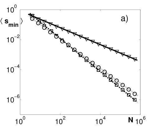
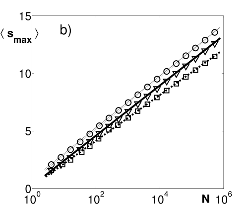
Figure 5: Dependence of the mean extremal spacing on the matrix size $N$. a) Mean minimal spacing $\langle s_{\min}\rangle$, assumed to behave as $N^{\eta}$ is plotted in log–log scale, and the fitted exponents read $\eta_{(P)}=-0.98$ for $\operatorname{CPE}_{N}$ ($\circ$) , $\eta_{(2)}=-1.09$ for $\operatorname{CUE}_{n\otimes n}$ ($\square$) , $\eta_{(k)}=-0.58$ for $\operatorname{CUE}_{2}^{\otimes k}$ ($\triangledown$). b) Mean maximal spacing $\langle s_{\max}\rangle$ assumed to behave as ${\kappa\log N}$ and plotted in log–linear scale, with fitted prefactors $\kappa_{(P)}=0.98$ for $\operatorname{CPE}_{N}$ ($\circ$) , $\kappa_{(2)}=0.85$ for $\operatorname{CUE}_{n\otimes n}$ ($\square$) , $\kappa_{(k)}=0.95$ for $\operatorname{CUE}_{2}^{\otimes k}$ ($\triangledown$). Symbols denote numerical results obtained for $2^{14}$ independent random matrices. Solid, dashed and dash-dot represent the fitted lines.

IV.1 Minimal spacings for tensor products

To analyze the distribution of the minimal spacing $P(s_{\rm min})$ for the tensor products of random unitary matrices it is convenient to introduce an auxiliary variable $y_{\min}=s_{\rm min}/\langle s_{\rm min}\rangle$. Probability distribution $P(y_{\rm min})$ is presented in Fig. 6 for the $n\times n$ systems with $n=2,3$ and $8$. Numerical results for $n=2$ agree with an explicit analytical prediction (3). Due to the tensor product structure of the ensemble the effect of level repulsion, characteristic of $\operatorname{CUE}$, is washed out.

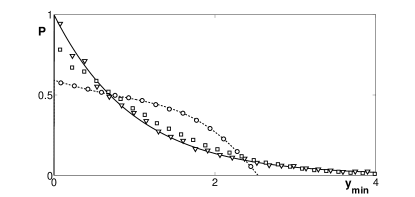
Figure 6: Probability densities $P(y_{\min})$ of the rescaled minimal spacing $y_{\min}=s_{\min}/\langle s_{\min}\rangle$ for tensor products of $\operatorname{CUE}$ random unitary matrices $\operatorname{CUE}_{n}\otimes\operatorname{CUE}_{n}$ for $n=2$ ($\circ$), $n=3$ ($\square$), and $n=8$ ($\triangledown$). The symbols denote numerical results obtained for $2^{14}$ independent matrices, solid curve represents the Poissonian distribution, while dashed line corresponds to eq. (3).

For larger $n$ the opposite effect of level clustering (large probability at small values of the minimal spacing) becomes stronger and already for $n=8$ probability distribution can be approximated by the exponential distribution, $P(y_{\rm min})=\exp(-y_{\rm min})$, typical of the Poissonian distribution. A similar transition from distribution (3) to the Poisson distribution occurs in the case of $k$-qubit systems, as shown in Fig. 7.

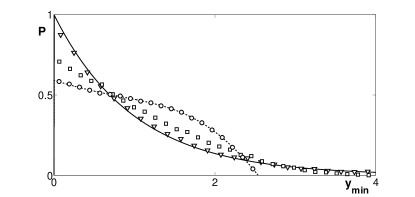
Figure 7: As in Fig. 6 for tensor products of $k$ independent Haar random unitary matrices of order two, ${CUE_{2}}^{\otimes k}$ for $k=2$ ($\circ$), $k=3$ ($\square$), and $k=8$ ($\triangledown$).

IV.2 Maximal spacings for tensor products

As in section III.4 we rescale the maximal spacing $s_{\rm max}$ and analyze the rescaled deviation from the expectation value

$$z_{\max}=\frac{\pi}{\sqrt{6\operatorname{Var}(s_{\max})}}\bigl{(}s_{\max}-\langle s_{\max}\rangle\bigr{)}.$$ (28)

The normalization factor is adjusted to predictions for the Poissonian process, for which the distribution of the variable $z$ is asymptotically described by the Gumbel distribution,

$$P(z)=e^{-(z+\gamma)-e^{-(z+\gamma)}}.$$ (29)

Recall that $\gamma\approx 0.5772$ denotes Euler’s constant, while the variance of the Gumbel distribution equal to $\pi^{2}/6$ suggests the convenient prefactor in the definition (28). Numerical results on the distributions of the variable $z_{\max}$ characterizing the distribution of the maximal spacings for the tensor products corresponding to two qunits and several qubits are presented in Fig. 6 and Fig. 8, respectively. In the asymptotic limit of a large matrix size numerical data seem to agree with predictions (29) of the Poisson ensemble.

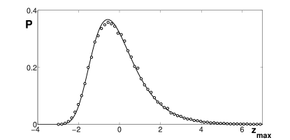
Figure 8: Distribution $P(z_{\max})$ of the deviations of the rescaled maximal spacing from the expected value, $z_{\max}=\alpha\bigl{(}s_{\max}-\langle s_{\max}\rangle\bigr{)}$ with $\alpha=\pi/\sqrt{6\operatorname{Var}(s_{\max})}$ for ensemble of $\operatorname{CUE}_{2^{6}\otimes 2^{6}}$ matrices ($\circ$). Numerical data obtained out of $2^{16}$ realizations while solid line denotes the Gumbel distribution (29).

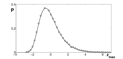
Figure 9: As in Fig. 8 for a sample of $10^{5}$ realizations of tensor products of $k=22$ random unitary matrices of order two.

V Concluding remarks

A significant and spectacular difference between the Poissonian ensemble on one side and $\operatorname{COE}$ and $\operatorname{CUE}$ on the other, concerning the degree of “repulsion” between adjacent levels can be effectively analyzed in terms of distributions of the extremal spacings. We analyzed the average minimal spacing for several ensembles of random unitary matrices. Basing on numerical results we propose a general form of the probability distribution $P(s_{min})$ of the minimal spacing for the standard ensembles of random unitary matrices. For $\operatorname{CUE}$ this distribution coincides with the recent result derived by Arous and Bourgade AB10 , while for $\operatorname{COE}$ it corresponds to the distributions analyzed for real symmetric matrices in CMD07 ; Fo10 .

The key part of this work concerned tensor products of random unitary matrices. In the case of $k$ independent random matrices of order $n$ distributed according to the Haar measure the tensor product leads asymptotically to a spectrum with Poissonian level spacing distribution TSKZZ12 ; Tk13 . However, we report here a different behavior for the statistics of the extreme spacings. Even though the mean largest spacing $\langle s_{max}\rangle$ can be described by predictions obtained for the Poisson ensemble of diagonal random unitary matrices of size $N=n^{k}$, this is not the case for the mean minimal spacings.

In particular, in the case of $k$ non-interacting qubits, described by the tensor product $CUE^{\otimes k}$, the mean minimal spacing $\langle s_{min}\rangle$ displays significant deviations with respect to the predictions of the Poisson ensemble. In the simplest case of a two qubit system we have shown that the eigenphases of the tensor product, $CUE_{2\otimes 2}$, show weaker repulsion than in the case of random CUE matrices of order $N=4$.

Our study leaves several questions open. In particular, numerical results encourage one to derive an unknown scaling law of the average minimal spacing $\langle s_{\min}\rangle$ in the case of $k$-qubit system. Furthermore, our observations suggesting that the distributions of the extremal spacing for ensembles of random matrices corresponding to two–qunit or $k$–qubit systems are asymptotically governed by the Poisson and the Gumbel distributions, respectively, should be confirmed by an analytical proof.

Appendix A Basic properties of the Poisson process

By a point process $\Xi$ on the real half-line $\mathbb{R}_{+}=[0,\infty)$ we mean a countable collection of random nonnegative numbers. For instance, a set $\Xi_{U}=\{(N/2\pi)\theta_{1},\ldots,(N/2\pi)\theta_{N}\}$ of the rescaled eigenvalues of a random unitary matrix $U$ can be viewed as a point process on $\mathbb{R}_{+}$.

A key example is a homogeneous Poisson point process $\Pi$ on $\mathbb{R}_{+}$ with a parameter $\lambda>0$ which is characterized by

1. for any pairwise disjoint and measurable subsets $B_{1},\ldots,B_{n}$ of $\mathbb{R}_{+}$ the number of points in these subsets form independent random variables,

2. for any measurable subset $B$ of $\mathbb{R}_{+}$ the number of points contained inside is described by the Poisson distribution with parameter $\lambda|B|$, where $|B|$ denotes the Lebesgue measure of $B$.

A detailed treatment of this process can be found in a classical monograph K . In this work we set the parameter $\lambda$ to $1$ and call it the standard Poisson point process.

One of the fundamental property of the Poisson process is that its spacings are independent and are described by exponential distributions. We read in K

Theorem 1.

Let $\Pi=\{X_{1},X_{2},\ldots\}$ be the standard Poisson point process, where the points are labeled so that they do not decrease. Define its spacings $Y_{1},Y_{2},\ldots$ by (7). Then the variables $Y_{1},Y_{2},\ldots$ are independent and identically distributed with density $e^{-y}$, $y>0$.

Knowing this we are able to examine the asymptotics of the extreme gaps $Y_{\min}=\min_{j\leq N}Y_{j}$ and $Y_{\max}=\max_{j\leq N}Y_{j}$.

Theorem 2.

Let $Y_{1},Y_{2},\ldots$ be a sequence of random variables which are independent identically distributed with density $P(y)=e^{-y}$ for $y>0$. Then,

$$\begin{split}\langle Y_{\min}\rangle&=\langle\min_{j\leq N}Y_{j}\rangle=1/N,\\ \langle Y_{\max}\rangle&=\langle\max_{j\leq N}Y_{j}\rangle=\sum_{k=1}^{N}1/k\sim\ln N.\end{split}$$ (30)

If we rescale the variables to set the mean to unity, $y=NY$, asymptotically they behave exponentially and concentrate respectively,

$$NY_{\min}\overset{d}{\longrightarrow}e^{-y}\textbf{1}_{\{y>0\}},$$ (31)

$$Y/\langle Y_{\min}\rangle\overset{d}{\longrightarrow}1,$$ (32)

where $\overset{d}{\longrightarrow}$ denotes the convergence in distribution.

Furthermore, the fluctuations of $Y/\langle Y_{\min}\rangle$ around $1$ are governed at the scale $\langle\max_{j\leq N}Y_{j}\rangle\sim\ln N$ by the Gumbel distribution,

$$Y-\langle Y_{\min}\rangle\overset{d}{\longrightarrow}P(z)=e^{-(z+\gamma)-e^{-(z+\gamma)}},$$ (33)

where $\gamma:=\lim_{n\to\infty}\left(\sum_{k=1}^{n}1/k-\ln n\right)\approx 0.5772$ is Euler’s constant.

Given the fact that the distribution functions are easily calculable,

$$\mathbb{P}\left(\min_{j\leq N}Y_{j}>t\right) =e^{-Nt},\quad t>0,$$

$$\mathbb{P}\left(\max_{j\leq N}Y_{j}\leq t\right) =(1-e^{-t})^{N},\quad t>0,$$

theorem 2 can be proved by a direct computation.

References

(1) F. Haake, Quantum Signatures of Chaos III ed. (Berlin,
Springer, 2006).
(2) H-J. Stöckman, Quantum Chaos (Cambridge, Cambridge
University Press, 1999).
(3) M. L. Mehta, Random matrices III ed. (Amsterdam,
Elsevier/Academic Press, 2004).
(4) A. Pandey and P. Shukla, Eigenvalue correlations in the
circular ensembles, J. Phys. A 24 3907 (1991).
(5) G. Lenz and K. Życzkowski, Time-reversal symmetry
breaking and the statistical properties of quantum systems, J. Phys. A
25, 5539 (1992).
(6) K. Życzkowski and M. Kuś, Interpolating
ensembles of random unitary matrices, Phys. Rev. E 53, 319 (1996).
(7) M. Poźniak, M. Kuś, and K. Życzkowski, Composed
ensembles of random unitary matrices, J. Phys. A 31, 1059 (1998).
(8) M. V. Berry and M. Robnik, Semiclassical level spacings
when regular and chaotic orbits coexist, J. Phys. A 17, 2413 (1984).
(9) P. J. Forrester, Log-gases and Random Matrices
(Princeton, Princeton University Press, 2010).
(10) G. Le Caër, C. Male, and R. Delannay, Nearest-neighbor spacing distributions of the -Hermite ensemble of random
matrices, Physica A 383, 190 (2007).
(11) G. B. Arous and P. Bourgade, Extreme gaps between
eigenvalues of random matrices preprint arXiv:1010.1294 (2010).
(12) T. Tkocz, M. Smaczyński, M. Kuś, Z. Zeitouni, and
K. Życzkowski, Tensor Products of Random Unitary Matrices, Random
Matrices: Theory and Appl.1, 1250009-26 (2012).
(13) A. Soshnikov, Statistics of extreme spacing in
determinantal random point processes, Mosc. Math. J. 5, 705 (2007).
(14) J.P. Vinson, Closest spacing of eigenvaluesPh.D.
thesis, Princeton University (2001).
(15) T. Tkocz, A note on the tensor product of two unitary
matrices, Electron. Commun. Probab. 18, 16, 1-7 (2013).
(16) F. Mezzadri, How to generate Random Matrices from the
Classical Compact Groups, Notices of the AMS 54, 592-604 (2007).
(17) J. F. C. Kingman, Poisson processes, Oxford Studies
in Probability, 3. (The Clarendon Press, Oxford University Press, New York, 1993).