Improved Randomized Online Scheduling of Intervals and Jobs

Abstract

We study the online preemptive scheduling of intervals and jobs (with restarts). Each interval or job has an arrival time, a deadline, a length and a weight. The objective is to maximize the total weight of completed intervals or jobs. While the deterministic case for intervals was settled a long time ago, the randomized case remains open. In this paper we first give a 2-competitive randomized algorithm for the case of equal length intervals. The algorithm is barely random in the sense that it randomly chooses between two deterministic algorithms at the beginning and then sticks with it thereafter. Then we extend the algorithm to cover several other cases of interval scheduling including monotone instances, C-benevolent instances and D-benevolent instances, giving the same competitive ratio. These algorithms are surprisingly simple but have the best competitive ratio against all previous (fully or barely) randomized algorithms. Next we extend the idea to give a 3-competitive algorithm for equal length jobs. Finally, we prove a lower bound of 2 on the competitive ratio of all barely random algorithms that choose between two deterministic algorithms for scheduling equal length intervals (and hence jobs).

keywords: interval and job scheduling; preemption with restart; online algorithms; randomized; lower bound

1 Introduction

In this paper, we study two online preemptive scheduling problems. In the interval scheduling problem, we are to schedule a set of weighted intervals which arrive online (in the order of their left endpoints) so that at any moment, at most one interval is being processed. We can abort the interval currently being processed in order to start a new one. The goal is to maximize the sum of the weights of completed intervals. The problem can be viewed as a job scheduling problem in which each job has, besides its weight, an arrival time, a length and a deadline. Moreover, the deadline is always tight, i.e., deadline always equals arrival time plus length. Thus, if one does not start an interval immediately upon its arrival, or if one aborts it before its completion, that interval will never be completed. The problem is fundamental in scheduling and is clearly relevant to a number of online problems such as call control and bandwidth allocation (see e.g., [2, 6, 19]).

We also study the more general problem of job scheduling with restart. Here, the deadline of a job needs not be tight and we can abort a job and restart it from the beginning some time later. Both problems are in fact special cases of the broadcast scheduling problem which gains much attention recently due to its application in video-on-demand, stock market quotation, etc (see e.g., [13, 18, 20]). In that problem, a server holding a number of pages receives requests from its clients and schedules the broadcasting of its pages. A request is satisfied if the requested page is broadcasted in its entirety after the arrival time and before the deadline of the request. The page currently being broadcasted can be aborted in order to start a new one, and the aborted page can be re-broadcasted from the beginning later. Interval and job scheduling with restart can be seen as a special case in which each request asks for a different page.

Our results concern barely random algorithms, i.e., randomized algorithms that randomly choose from a very small (constant) number of deterministic algorithms at the beginning and then stick with it thereafter. Quite some previous work in online scheduling considered the use of barely random algorithms (see e.g. [1, 9, 17]); it is interesting to consider how the competitiveness improves (upon their deterministic counterparts) by combining just a few deterministic algorithms. From now on, whenever we refer to “barely random algorithms”, we mean algorithms that choose between two deterministic algorithms but possibly with unequal probability.

Types of instances.

In this paper, we consider the following special types of intervals or jobs:

1. equal length instances where all intervals or jobs have the same length,

2. monotone instances where intervals arriving earlier also have earlier deadlines, and

3. C- and D-benevolent instances where the weight of an interval is given by some ‘nice’ function of its length (convex increasing for C-benevolent, and decreasing for D-benevolent).

The models will be defined precisely in the next section. These cases are already highly non-trivial, as we will see shortly, and many previous works on these problems put further restrictions on the inputs (such as requiring jobs to be unweighted or arrival times to be integral, in addition to being equal-length). The power of randomization for these problems is especially unclear.

1.1 Previous work

The general case where intervals can have arbitrary lengths and weights does not admit constant competitive algorithms [19], even with randomization [6]. Therefore, some special types of instances have been studied in the literature.

We first mention results for equal length interval scheduling. The deterministic case was settled in [19] where a 4-competitive algorithm and a matching lower bound were given. Miyazawa and Erlebach [16] were the first to give a better randomized algorithm: its competitive ratio is 3 but it only works for a special case where the weights of the intervals form a non-decreasing sequence. They also gave the first randomized lower bound of 5/4. The first randomized algorithm for arbitrary weight that has competitive ratio better than 4 (the bound for deterministic algorithms) was devised in [12]. It is 3.618-competitive and is barely random, choosing between two deterministic algorithms with equal probability. In the same paper, a lower bound of 2 for such barely random algorithms and a lower bound of 4/3 for general randomized algorithms were also proved. Recently, Epstein and Levin [11] gave a 2.455-competitive randomized algorithm and a 3.227-competitive barely random algorithm. They also gave a 1.693 lower bound on the randomized competitive ratio.

The class of monotone instances (also called similarly ordered [9] or agreeable [15] instances in the literature) is a generalization of the class of equal length instances. Therefore, the former class inherits all the lower bounds for the latter class. In the offline case, the class of monotone instances is actually equivalent to that of equal length instances because of the result (see e.g. [4]) that the class of proper interval graphs (intersection graphs of intervals where no interval is strictly contained in another) is equal to the class of unit interval graphs. In the online case however, it is not completely clear that such an equivalence holds although some of the algorithms for the equal length case also work for the monotone case (e.g. [16, 12, 11]).

Some of the aforementioned results for equal length instances also work for C- and D-benevolent instances, including Woeginger’s 4-competitive deterministic algorithm, the lower bound of 4/3 in [12], the upper bounds in [11] (for D-benevolent instances only) and the lower bound in [11] (for C-benevolent instances only; they gave another slightly weaker lower bound of 3/2 for D-benevolent instances). A 3.732-competitive barely random algorithm for C-benevolent instances was given by Seiden [17]. Table 1 summarizes the various upper and lower bounds for randomized interval scheduling.

upper bound lower bound equal length 2.455 [11] 1.693 [11] 3.227 (barely random) [11] 2 (barely random) [this paper] 2 (barely random) [this paper] monotone same as above same as above C-benevolent 3.732 [17] 1.693 [11] 2 (barely random) [this paper] D-benevolent 2.455 [11] 1.5 [11] (with a surjective condition) 3.227 (barely random) [11] 2 (barely random) [this paper]

Table 1: Best previous and new results for randomized interval scheduling

Next we consider the problem of job scheduling with restarts. Zheng et al. [20] gave a 4.56-competitive deterministic algorithm. The algorithm was for the more general problem of scheduling broadcasts but it works for jobs scheduling with restarts too. We are not aware of previous results in the randomized case. Nevertheless, Chrobak et al. [9] considered a special case where the jobs have no weights and the objective is to maximize the number of completed jobs. For the randomized nonpreemptive case they gave a 5/3-competitive barely random algorithm and a lower bound of 3/2 for barely random algorithms that choose between two deterministic algorithms. They also gave an optimal 3/2-competitive algorithm for the deterministic preemptive (with restart) case, and a lower bound of 6/5 for the randomized preemptive case.

We can also assume that the time is discretized into unit length slots and all (unit) jobs can only start at the beginning of each slot. Being a special case of the problem we consider in this paper, this version of unit job scheduling has been widely studied and has applications in buffer management of QoS switches. For this problem, a $e/(e-1)$-competitive randomized algorithm was given in [7], and a randomized lower bound of 1.25 was given in [8]. The current best deterministic algorithm is 1.828-competitive [10].

An alternative preemption model is to allow the partially-executed job to resume its execution from the point that it is preempted. This was studied, for example, in [3, 14].

1.2 Our results

In this paper we give new randomized algorithms for the different versions of the online interval scheduling problem. They are all barely random and have a competitive ratio of 2. Thus they substantially improve previous results. See Table 1. It should be noted that although the algorithms are fairly simple, they were not discovered in several previous attempts by other researchers and ourselves [11, 12, 16]. Moreover the algorithms for all these versions of the problem are based on the same idea, which gives a unified way of analyzing these algorithms that were not present in previous works.

Next we extend the algorithm to the case of job scheduling (with restarts), and prove that it is 3-competitive. This is the first randomized algorithm we are aware of for this problem. The extension of the algorithm is very natural but the proof is considerably more involved.

Finally we prove a lower bound of 2 for barely random algorithms for scheduling equal length intervals (and jobs) that choose between two deterministic algorithms, not necessarily with equal probability. Thus it matches the upper bound of 2 for this class of barely random algorithms. Although this lower bound does not cover more general classes of barely random or randomized algorithms, we believe that this is still of interest. For example, a result of this type appeared in [9]. Also, no barely random algorithm using three or more deterministic algorithms with a better performance is known. The proof is also much more complicated than the one in [12] with equal probability assumption.

2 Preliminaries

A job $J$ is specified by its arrival time $r(J)$, its deadline $d(J)$, its length (or processing time) $p(J)$ and its weight $w(J)$. All $r(J),d(J),p(J)$ and $w(J)$ are nonnegative real numbers. An interval is a job with tight deadline, i.e. $d(J)=r(J)+p(J)$. We further introduce the following concepts for intervals: for intervals $I$ and $J$ with $r(I)<r(J)$, $I$ contains $J$ if $d(I)\geq d(J)$; if $r(J)<d(I)<d(J)$, the two intervals overlap; and if $d(I)\leq r(J)<d(J)$, the intervals are disjoint.

Next we define the types of instances that we consider in this paper. The equal length case is where $p(J)$ is the same for all $J$; without loss of generality we can assume $p(J)=1$. The remaining notions apply to intervals only. An instance is called monotone if for any two intervals $I$ and $J$, if $r(I)<r(J)$ then $d(I)\leq d(J)$. An instance is called C-benevolent if the weights of intervals are given by a function $f$ of their lengths, where the function $f$ satisfies the following three properties:

(i)

$f(0)=0$ and $f(p)>0$ for all $p>0$,

(ii)

$f$ is strictly increasing, and

(iii)

$f$ is convex, i.e. $f(p_{1})+f(p_{2})\leq f(p_{1}-\epsilon)+f(p_{2}+\epsilon)$ for $0<\epsilon\leq p_{1}\leq p_{2}$.

Finally, an instance is called D-benevolent if the weights of intervals are given by a function $f$ of their lengths where

(i)

$f(0)=0$ and $f(p)>0$ for any $p>0$, and

(ii)

$f$ is decreasing in $(0,\infty)$.

In our analysis, we partition the time axis into segments called slots, $s_{1},s_{2},\ldots$, such that each time instant belongs to exactly one slot and the union of all slots cover the entire time axis. The precise way of defining the slots depends on the case being studied (equal-length, monotone, C- or D-benevolent instances). Slot $s_{i}$ is an odd slot if $i$ is odd, and is an even slot otherwise.

The following is an important, though perhaps unusual, definition used throughout the paper. We say that a job (or an interval) is accepted by an algorithm $A$ in a slot $s$ if it is started by $A$ within the duration of slot $s$ and is then completed without interruption. Note that the completion time may well be after slot $s$. $A$ may start more than one job in a slot, but it will become clear that for all online algorithms that we consider, at most one job will be accepted in a slot; all other jobs that were started will be aborted. For $OPT$ we can assume that it always completes each interval or job it starts.

The value of a schedule is the total weight of the jobs that are completed in the schedule. The performance of online algorithms is measured using competitive analysis [5]. An online randomized algorithm $A$ is $c$-competitive if the expected value obtained by $A$ is at least $1/c$ the value obtained by the optimal offline algorithm, for any input instance. The infimum of all such $c$ is called the competitive ratio of $A$. We use $OPT$ to denote the optimal algorithm (and its schedule).

3 Algorithms for Scheduling Intervals

3.1 Equal Length Instances

In this section we describe and analyse a very simple algorithm $RAN$ for the case of equal length intervals. $RAN$ is barely random and consists of two deterministic algorithms $A$ and $B$, described as follows. The time axis is divided into unit length slots, $s_{1},s_{2},\ldots$, where slot $s_{i}$ covers time [$i-1,i$) for $i=1,2,\ldots$. Intuitively, $A$ takes care of odd slots and $B$ takes care of even slots. Within each odd slot $s_{i}$, $A$ starts the interval arriving first. If a new interval arrives in this slot while an interval is being processed, $A$ will abort and start the new interval if its weight is larger than the current interval; otherwise the new interval is discarded. At the end of this slot, $A$ is running (or about to complete) an interval with the largest weight among those that arrive within $s_{i}$; let $I_{i}$ denote this interval. $A$ then runs $I_{i}$ to completion without abortion during the next (even) slot $s_{i+1}$. (Thus, $I_{i}$ is the only interval accepted by $A$ in slot $s_{i}$.) Algorithm $A$ then stays idle until the beginning of the next odd slot. $B$ runs similarly on even slots. $RAN$ chooses one of $A$ and $B$ with equal probability 1/2 at the beginning.

Theorem 3.1

$RAN$ is $2$-competitive for online interval scheduling on equal length instances.

Proof. Each $I_{i}$ is accepted by either $A$ or $B$. Therefore, $RAN$ completes each $I_{i}$ with probability 1/2. On the other hand, $OPT$ can accept at most one interval in each slot $s_{i}$, with weight at most $w(I_{i})$. It follows that the total value of $OPT$ is at most 2 times the expected value of $RAN$. $\Box$

Trivial examples can show that $RAN$ is not better than 2-competitive (e.g. a single interval). In fact we will show in Section 5 that no barely random algorithm that chooses between two deterministic algorithms is better than 2-competitive. But first we consider how this result can be generalized to other types of instances.

3.2 Monotone Instances

Algorithm $RAN$-$M$.

We adapt the idea of $RAN$ to the case of monotone instances and call the algorithm $RAN$-$M$. Similar to $RAN$, $RAN$-$M$ consists of two deterministic algorithms $A$ and $B$, each chosen to execute with probability 1/2 at the beginning. The difference is that we cannot use the idea of unit length slots but we must define the lengths of the slots in an online manner.

The execution of the algorithm is divided into phases and we name the slots in each phase locally as $s_{1},s_{2},\ldots$ independent of other phases. After the end of a phase and before the beginning of the next phase, the algorithm (both $A$ and $B$) is idle with no pending intervals. A new phase starts when the first interval arrives while the algorithm is idle. Among all intervals that arrive at this time instant, let $I_{0}$ be the one with the earliest deadline (ties broken arbitrarily). Then slot $s_{1}$ is defined as $[r(I_{0}),d(I_{0}))$. $A$ aims to accept the heaviest interval among those with arrival time falling within slot $s_{1}$. To do this, $A$ simply starts the first interval arriving in $s_{1}$, and then whenever a new interval arrives that is heavier than the interval that $A$ is currently executing, $A$ aborts the current one and starts the new heavier interval. This is repeated until the time $d(I_{0})$ is reached. By the property of monotone instances and the choice of $I_{0}$, these intervals all have finishing time on or after $d(I_{0})$. Let $I_{1}$ denote the interval that $A$ is executing (or about to complete) at the end of slot $s_{1}$, i.e., time $d(I_{0})$. $B$ remains idle during the whole slot. If $A$ just finishes $I_{1}$ at time $d(I_{0})$, then it will become idle again and this phase ends. Otherwise, $d(I_{1})>d(I_{0})$ and slot $s_{2}$ is now defined as $[d(I_{0}),d(I_{1}))$.

In slot $s_{2}$, $A$ continues to execute $I_{1}$ to completion without any interruption. (Thus, $I_{1}$ is the only interval accepted by $A$ in slot $s_{1}$.) $B$ accepts the heaviest interval among those with arrival time falling within slot $s_{2}$, in the same manner $A$ did in the previous slot. This interval is denoted by $I_{2}$ and $B$ will run it to completion during slot $s_{3}$ (if its deadline is after the end of slot $s_{2}$).

In general, slot $s_{i}$ (where $i>1$) is defined as $[d(I_{i-2}),d(I_{i-1}))$. If $i$ is odd, then at the beginning of slot $s_{i}$, $B$ is executing $I_{i-1}$ (the interval accepted by $B$ in slot $s_{i-1}$) and $A$ is idle. $B$ will run $I_{i-1}$ to completion while $A$ will accept the heaviest interval among those arriving during this slot. If $i$ is even, the actions are the same except that the roles of $A$ and $B$ are reversed.

Theorem 3.2

RAN-M is $2$-competitive for online interval scheduling on monotone instances.

Proof. No interval will arrive during the idle time between phases (since otherwise $RAN$-$M$ would have started a new phase), so each phase can be analyzed separately. Each interval completed by $OPT$ will be analyzed according to the slot its arrival time falls into.

In each slot $s_{i}$, $OPT$ can accept at most one interval: This is true for $s_{1}$ by the way $s_{1}$ is chosen. For $i>1$, consider the first interval $I^{\prime}$ accepted by $OPT$ in slot $s_{i}=[d(I_{i-2}),d(I_{i-1}))$. (Recall that accepting a job means starting the job and then executing it to completion without interruption.) Since the start of slot $s_{i}$ is after $r(I_{i-1})$, we have $r(I^{\prime})>r(I_{i-1})$. By the monotone property, $d(I^{\prime})\geq d(I_{i-1})$. So, $OPT$ cannot accept another interval in slot $s_{i}$. The rest of the proof is the same as the equal length case, namely, that the interval accepted by $OPT$ in each slot has weight at most that of the interval accepted by $A$ or $B$ in the same slot. It follows that $RAN$-$M$ is 2-competitive. $\Box$

3.3 C-benevolent Instances

Algorithm $RAN$-$C$.

Once again, the algorithm for C-benevolent instances $RAN$-$C$ consists of two deterministic algorithms $A$ and $B$, each with probability 1/2 of being executed. The execution of the algorithm is divided into phases as in the monotone case.

When a new phase begins, the earliest arriving interval, denoted by $I_{0}$, defines the first slot $s_{1}$, i.e., $s_{1}=[r(I_{0}),d(I_{0}))$. (If there are several intervals arriving at the same time, let $I_{0}$ be the one with the longest length.) We first describe the processing of intervals in slot $s_{1}$, which is slightly different from the other slots. First, $B$ starts and completes $I_{0}$. During $s_{1}$, $A$ accepts the longest interval among those with arrival time during $(r(I_{0}),d(I_{0}))$ and finishing time after $d(I_{0})$. Denote this interval by $I_{1}$. (Note that there may be other intervals that arrive and end before $I_{1}$ arrives. Naturally, $A$ could finish them in order to gain more value. However, to simplify our analysis, we assume that $A$ will not process them.) If there is no such $I_{1}$, i.e., no interval arrives within $s_{1}$ and ends after $d(I_{0})$, the phase ends at the end of $s_{1}$.

Suppose $I_{1}$ exists. Then define slot $s_{2}$ as $[d(I_{0}),d(I_{1}))$. $A$ uses the entire slot $s_{2}$ to complete $I_{1}$ without interruption. After completing $I_{0}$ at time $d(I_{0})$, $B$ accepts the longest interval (denoted $I_{2}$) among those arriving within slot $s_{2}$ and finishing after $d(I_{1})$, in a way similar to the action of $A$ in the previous slot. Again, if such an $I_{2}$ does not exist, the phase ends at the end of $s_{2}$. Otherwise, slot $s_{3}$ is defined as $[d(I_{1}),d(I_{2}))$ and $B$ will complete $I_{2}$ that ends after $d(I_{1})$. Similarly, after $A$ finishes $I_{1}$ in time $d(I_{1})$, it starts the longest interval (denoted by $I_{3}$) arriving during $s_{3}$ and finishing after $d(I_{2})$, and so on.

In general, slot $s_{i}$ (for $i>1$) is defined as $[d(I_{i-2}),d(I_{i-1}))$. If $i$ is odd, then $B$ takes the entire slot to complete the interval $I_{i-1}$ without interruption while $A$ accepts the longest interval $I_{i}$ that arrives during slot $s_{i}$ and ends after $d(I_{i-1})$. If $i$ is even then the roles of $A$ and $B$ are reversed.

Competitive Analysis.

We first state the following useful lemma which holds for any C-benevolent function $f$.

Lemma 3.1

For any C-benevolent function $f$, given any $k+1$ positive real numbers $p_{i}$ $(1\leq i\leq k)$ and $P$, if $P\geq\sum^{k}_{i=1}p_{i}$, then $f(P)\geq\sum^{k}_{i=1}f(p_{i})$.

Proof. $f(P)\geq f(\sum^{k}_{i=1}p_{i})\geq f(p_{1})+f(\sum^{k}_{i=2}p_{i})\geq\sum^{2}_{i=1}f(p_{i})+f(\sum^{k}_{i=3}p_{i})\geq\ldots\geq\sum^{k}_{i=1}f(p_{i})$. $\Box$

Theorem 3.3

$RAN$-$C$ is $2$-competitive for online interval scheduling on C-benevolent instances.

Proof. As a first step to the proof we simplify the $OPT$ schedule. Within each slot $s_{i}$ in a phase, $i\geq 1$, $OPT$ starts a sequence of disjoint intervals (in increasing order of starting times) $\mathcal{O}_{i}=\{o_{i,1},o_{i,2},\ldots,o_{i,k_{i}}\}$. Only the last interval, $o_{i,k_{i}}$, may end later than $d(I_{i-1})$ (the ending time of $s_{i}$). If it does, then we merge $o_{i,1},o_{i,2},\ldots,o_{i,k_{i}-1}$ into one interval $pre_{i}$ such that $r(pre_{i})=r(o_{i,1})$ and $d(pre_{i})=r(o_{i,k_{i}})$, and thus $p(pre_{i})=r(o_{i,k_{i}})-r(o_{i,1})\geq\sum^{k_{i}-1}_{j=1}p(o_{i,j})$. By Lemma 3.1, $f(p(pre_{i}))\geq\sum^{k_{i}-1}_{j=1}f(p(o_{i,j}))$. Otherwise, (i.e. $o_{i,k_{i}}$ ends before $d(I_{i-1})$), we merge all the intervals in $\mathcal{O}_{i}$ into one interval $pre_{i}$ such that $r(pre_{i})=r(o_{i,1})$ and $p(pre_{i})=d(o_{i,k_{i}})-r(o_{i,1})\geq\sum^{k_{i}}_{j=1}p(o_{i,j})$. Thus, in both cases, such merging can only make $OPT$’s value larger. So we can assume that $OPT$ starts at most two intervals $pre_{i}$ and $o_{i,k_{i}}$ in slot $s_{i}$. After understanding the notations, we simply denote the two intervals $pre_{i}$ and $o_{i,k_{i}}$ by $o_{i,1}$ and $o_{i,2}$, respectively.

The interval $o_{i,1}$ (if exist) is contained in $I_{i-1}$ and so $p(o_{i,1})\leq p(I_{i-1})$. The interval $o_{i,2}$ (if exist) will end after $d(I_{i-1})$, and $p(o_{i,2})\leq p(I_{i})$ since $I_{i}$ is defined to be the longest interval that arrives during slot $s_{i}$ and ends after $d(I_{i-1})$. Note that $o_{i,2}$ may also end after $d(I_{i+l})$ for some $l\geq 0$. In this case, neither $o_{v,1}$ nor $o_{v,2}$ exist for $i\leq v\leq i+l$. If any $o_{i,1}$ or $o_{i,2}$ does not exist, we set its length to zero.

We now analyze the competitive ratio of $RAN$-$C$. As in the monotone case, each phase can be analyzed separately. Consider an arbitrary schedule $S=\{I_{0},I_{1},\ldots,I_{n-1}\}$ produced by $RAN$-$C$ in a phase with $n\geq 1$ slots, where $I_{i}$ overlaps $I_{i+1}$ $(0\leq i<n-1)$, and the corresponding schedule $S^{*}=\{o_{1,1},o_{1,2},o_{2,1},\ldots,o_{n,1}\}$ produced by $OPT$ as $RAN$-$C$ produces $S$. (Note that $o_{n,2}$ cannot exist since otherwise this means there are some intervals that arrive within $[d(I_{n-2}),d(I_{n-1}))$ and end after $d(I_{n-1})$, and hence the phase will not end and $RAN$-$C$ will start an $I_{n}$.)

For each slot $i$, $OPT$ starts two intervals $o_{i,1}$ and $o_{i,2}$ while $RAN$-$C$ accepts $I_{i-1}$. For presentation convenience, let $x_{i,1}=p(o_{i,1})$, $x_{i,2}=p(o_{i,2})$ and $y_{i}=p(I_{i})$. We already have that $x_{i,1}\leq y_{i-1}$ for $1\leq i\leq n$ and $x_{i,2}\leq y_{i}$ for $1\leq i<n$. We will show that

$$\sum^{n}_{i=1}f(x_{i,1})+\sum^{n-1}_{i=1}f(x_{i,2})\leq\sum^{n-1}_{i=0}f(y_{i}).$$ (1)

The left hand side of (1) represents the total weight of intervals in $S^{*}$ (note that $o_{n,2}$ does not exist) while the right hand side represents the total weight of intervals in $S$. Since $RAN$-$C$ completes each interval in $S$ with probability 1/2, its expected value is half of the right hand side of (1). Thus by proving (1) we show the 2-competitiveness of $RAN$-$C$.

We prove (1) by induction on $n$. When $n=1$, (1) reduces to $f(x_{1,1})\leq f(y_{0})$ which is true since $x_{1,1}\leq y_{0}$. Assume the claim holds for $n=k-1$, i.e., $\sum^{k-1}_{i=1}f(x_{i,1})+\sum^{k-2}_{i=1}f(x_{i,2})\leq\sum^{k-2}_{i=1}f(y_{i})$. Consider $I_{k}$, $o_{k-1,2}$ and $o_{k,1}$. We have $x_{k-1,2}\leq y_{k-1}$ and $x_{k,1}\leq y_{k-1}$. If $x_{k-1,2}+x_{k,1}\leq y_{k-1}$, then $f(x_{k-1,2})+f(x_{k,1})\leq f(x_{k-1,2}+x_{k,1})\leq f(y_{k-1})$. Adding this to the induction hypothesis gives $\sum^{k}_{i=1}f(x_{i,1})+\sum^{k-1}_{i=1}f(x_{i,2})\leq\sum^{k-1}_{i=0}f(y_{i})$ and thus the claim holds for $n=k$.

Otherwise, if $x_{k-1,2}+x_{k,1}>y_{k-1}$, we first change the schedule $S^{*}$ as follows: we increase the length of $x_{k,1}$ to $y_{k-1}$ and decrease the length of $x_{k-1,2}$ by the same amount. The corresponding $r(o_{k-1,2})$ and $d(o_{k,1})$ are fixed while both $d(o_{k-1,2})$ and $r(o_{k,1})$ decrease by an amount of $y_{k-1}-x_{k,1}$. $OPT$ will only get better since $f(x_{k,1})+f(x_{k-1,2})\leq f(y_{k-1})+f(x_{k-1,2}-(y_{k-1}-x_{k,1}))$ by the properties of C-benevolent functions. After this change, $I_{k-1}$ and $o_{k,1}$ have the same length. The new $o_{k-1,2}$ now ends on or before $d(I_{k-2})$. We merge the new $o_{k-1,2}$ into $o_{k-1,1}$ so that the new $o_{k-1,1}$ extends its length to $x_{k-1,2}+x_{k-1,1}$ and keeps its start time $r(o_{k-1,1})$ unchanged. In the case that $x_{k-1,1}=0$ before merging $o_{k-1,2}$, we set $r(o_{k-1,1})=r(o_{k-1,2})$. The new $o_{k-1,1}$ is still contained by $I_{k-2}$ and thus $x_{k-1,1}\leq y_{k-2}$ still holds. After merging, $x_{k-1,2}=0$ and $x_{k,1}=y_{k-1}$. Therefore $\sum^{k}_{i=1}f(x_{i,1})+\sum^{k-1}_{i=1}f(x_{i,2})=\sum^{k-1}_{i=1}f(x_{i,1})+\sum^{k-2}_{i=1}f(x_{i,2})+f(x_{k,1})\leq\sum^{k-2}_{i=0}f(y_{i})+f(y_{k-1})=\sum^{k-1}_{i=0}f(y_{i})$. Thus the claim is true for $n=k$. $\Box$

3.4 D-benevolent Instances

Algorithm $RAN$-$D$.

The basic idea of $RAN$-$D$ is same as $RAN$: two algorithms $A$ or $B$ are executed each with probability 1/2. Intuitively, in an odd slot (where slots will be defined precisely in the following paragraphs), $A$ accepts the largest-weight interval arriving during that slot, by starting an interval and preempting if a new one arrives with a larger weight. We call the interval being executed by $A$ the main interval, denoted by $I_{M}$. Meanwhile, $B$ continues to run to completion the interval started in the previous slot; we call this the residual interval, denoted by $I_{R}$. This residual interval must be completed (as in the equal length case) because this is the interval accepted in the previous slot. However in the D-benevolent case, if a shorter (and therefore larger weight) interval arrives, the residual interval can actually be preempted and replaced by this new interval. For even slots the roles of $A$ and $B$ are reversed (and the interval started by $B$ is the main interval and the one completed by $A$ the residual interval).

Unlike $RAN$-$M$ or $RAN$-$C$, here when slot $s_{i-1}$ finishes, the next slot $s_{i}$ is not completely determined: slot $s_{i}$ begins where $s_{i-1}$ ends, but the ending time of slot $s_{i}$ will only get a provisional value, which may become smaller (but not larger) later on. This is called the provisional ending time of the slot, denoted by $e_{i}$. Slots will also be grouped into phases as in the other types of instances.

Note that $I_{M}$, $I_{R}$ and $e_{i}$ change during the execution of the algorithm, even within the same slot. But $RAN$-$D$ always maintains the following invariant:

Invariant: Suppose $I_{R}$ and $I_{M}$ are the residual and main interval respectively during execution in a slot $s_{i}$. Then $e_{i}=d(I_{R})\leq d(I_{M})$ (if the intervals exist). Moreover $e_{i}$ can only be decreased, not increased.

We describe the processing of intervals in a slot $s_{i}$ ($i\geq 1$). Consider an odd slot $s_{i}$ (the case of even slots is the same with the roles of $A$ and $B$ reversed). At the beginning of $s_{i}$, $A$ is idle and $B$ is continuing the execution of a residual interval $I_{R}$. At this point $e_{i}$ is provisionally set to $d(I_{R})$. In the case of the first slot, there is no residual interval left over from the previous slot, so we set $e_{i}$ to be the deadline of the first interval that arrives. If more than one interval arrive at the same instant, choose anyone.

Consider a time during $s_{i}$ when an interval $I$ arrives while $A$ and $B$ are respectively executing some intervals $I_{M}$ and $I_{R}$. If more than one interval arrive at the same instant, process them in any order. If $A$ or $B$ is idle, assume $I_{M}$ or $I_{R}$ to have weight 0. Then $A$ and $B$ react according to the following three cases:

1. If $d(I)\geq e_{i}$ and $w(I)>w(I_{M})$, then $I$ preempts $I_{M}$, and this $I$ becomes the new $I_{M}$. In this case, $e_{i}$ remains unchanged.

2. If $d(I)<e_{i}$ (which implies $w(I)\geq w(I_{M})$ and $w(I)\geq w(I_{R})$ because by the invariant, $d(I_{M})\geq d(I_{R})=e_{i}>d(I)$, and $I$ arrives no earlier than either $I_{M}$ or $I_{R}$, and thus $I$ is shorter), then $I$ preempts both $I_{M}$ in $A$ and $I_{R}$ in $B$. Here $I$ becomes the new $I_{M}$ and $I_{R}$, and $e_{i}$ is then set to $d(I)$.

3. Otherwise, $w(I)\leq w(I_{M})$ and $I$ is discarded.

Observe that the invariant is always maintained when we change any of $I_{M}$, $I_{R}$ or $e_{i}$.

This process repeats until time $e_{i}$ is reached and slot $s_{i}$ ends. If $d(I_{M})>e_{i}$ at the end of slot $s_{i}$, then a new slot $s_{i+1}$ begins where slot $s_{i}$ ends. $A$ has not finished execution of $I_{M}$ yet, so it now becomes the $I_{R}$ of slot $s_{i+1}$, and $e_{i+1}$ is provisionally set to $d(I_{R})$. Otherwise, $d(I_{M})=e_{i}$ and $A$ just finishes execution of $I_{M}$, then the phase ends. In this case we wait until the next interval arrival, then a new phase starts.

Note that $RAN$-$D$ needs to simulate the execution of both $A$ and $B$ (to determine when slots end) but the actual execution follows only one of them.

Theorem 3.4

$RAN$-$D$ is $2$-competitive for online interval scheduling on D-benevolent instances.

Proof. Consider each slot $s_{i}=[e_{i-1},e_{i})$. We claim that $OPT$ can start at most one interval in $s_{i}$ and that this interval cannot finish strictly before $e_{i}$. The first part of the claim follows from the second since if $OPT$ starts two or more intervals within $s_{i}$, then the first such interval must end strictly before $e_{i}$. Assume to the contrary that $OPT$ starts an interval $I$ that finishes strictly before $e_{i}$. Then $I$ also finishes strictly before the provisional value of $e_{i}$ at the moment $I$ arrives, since the provisional ending time only decreases. By the design of the algorithm, at that point $e_{i}$ will be reduced to $d(I)$. $e_{i}$ may be reduced further subsequently, but in any case this contradicts the fact that $d(I)<e_{i}$. Hence the claim follows.

Now suppose $OPT$ starts an interval $I$ in an odd slot $s_{i}$ and eventually completes it. We will show that if $s_{i}$ is not the last slot in the phase, $A$ will complete an interval of weight no less than $w(I)$ in slot $s_{i+1}$; if $s_{i}$ is the last slot, then $A$ will complete an interval of weight no less than $w(I)$ in slot $s_{i}$.

Consider the moment when $I$ arrives in $s_{i}$. If $I$ has larger weight than the current $I_{M}$, $A$ will preempt it and start $I$. Thus, by the end of $s_{i}$, $A$ should have started a main interval $I_{M}$ of weight at least $w(I)$. If this is the last slot, then $A$ completes $I_{M}$ at the end of $s_{i}$. Otherwise, $I_{M}$ becomes the residual interval in slot $s_{i+1}$ and $A$ will execute it to completion (as an residual interval) in $s_{i+1}$ unless another interval $I^{\prime}$ arrives in $s_{i+1}$ such that $d(I^{\prime})<e_{i+1}$ (and hence $w(I^{\prime})\geq w(I_{M})$). Note that $e_{i+1}$ will then be reduced to $d(I^{\prime})$. This $I^{\prime}$ may still be preempted by intervals of even larger weight and earlier deadline. In any case, at exactly the end of the next slot $s_{i+1}$, $A$ would have completed the residual interval.

We can make a similar claim for even slots. Therefore it follows that, for every interval started by $OPT$, either $A$ or $B$ will complete an interval of at least the same weight in the same or the next slot. Thus the total value of $A$ and $B$ is no less than that of $OPT$. The 2-competitiveness then follows since each of A/B is executed with 1/2 probability. $\Box$

4 Algorithms for Equal Length Jobs

Algorithm $RAN$-$J$.

In this section we extend $RAN$ to the online scheduling of equal length jobs with restarts. The algorithm remains very simple but the analysis is more involved. Again $RAN$-$J$ chooses between two deterministic algorithms $A$ and $B$, each with probability 1/2, and again $A$ takes care of odd slots and $B$ takes care of even slots, where the slots are defined as in the equal length interval case (i.e. they all have unit length). At the beginning of each odd slot, $A$ considers all pending jobs that can still be completed, and starts the one with the largest weight. (If there are multiple jobs with the same maximum weight, start an arbitrary one.) If another job of a larger weight arrives within the slot, $A$ aborts the current job and starts the new one instead. At the end of this odd slot, the job that is being executed will run to completion (into the following even slot) without abortion. $A$ will then stay idle until the beginning of the next odd slot. Even slots are handled by $B$ similarly.

The following simple example (see Figure 1(a)) illustrates the algorithm, and shows that $RAN$-$J$ is not better than 3-competitive. Consider three jobs $X,Y,Z$, where $r(X)=0,d(X)=3,w(X)=1+\epsilon$ for arbitrary small $\epsilon>0$; $r(Y)=0,d(Y)=1,w(Y)=1$; and $r(Z)=1,d(Z)=2,w(Z)=1$. Both $A$ and $B$ will complete $X$ only, but $OPT$ can complete all three.

Notations.

We define some additional notations that will be used in the rest of this section to make our discussion clearer. The notation $[s_{1}..s_{2}]$ denotes a range of slots from slot $s_{1}$ to $s_{2}$ inclusive, where $s_{1}$ is before $s_{2}$. Arithmetic operators on slots carry the natural meaning, so $s+1$ is the slot immediately after $s$, $s-1$ is the slot immediately before $s$, $s_{1}<s_{2}$ means $s_{1}$ is before $s_{2}$, etc. The job accepted by an algorithm $A$ in slot $s$ is denoted by $A(s)$. (Any algorithm can accept at most one job in each slot since the slot has the same length as a job.) We define the inverse $A^{-1}(x)$ to be the slot $s$ with $A(s)=x$, if it exists; otherwise it is undefined.

Charging scheme.

Our approach to the proof is to map (or charge) the weights of jobs accepted by $OPT$ to slots where $A$ or $B$ have accepted ‘sufficiently heavy’ jobs; namely, that each slot $s$ receives a charge at most 1.5 times of $w(A(s))$ or $w(B(s))$. In some cases this is not possible and we pair up slots with large charges with slots with small charges so that the overall ratio is still at most 1.5. Since each job in $A$ or $B$ is completed with probability 1/2 only, the expected value of the online algorithm is half the total value of $A$ and $B$. This gives a competitiveness of 3.

The charging scheme is defined as follows. Consider a slot $s$ where $OPT$ accepts the job $OPT(s)$. Suppose $s$ is odd (so $A$ is choosing the heaviest job to start). If $w(A(s))\geq w(OPT(s))$, charge the weight of $OPT(s)$ to $s$. We call this a downward charge. Otherwise, $A$ must have accepted $OPT(s)$ at some earlier slot $s^{\prime}$. Charge half the weight of $OPT(s)$ to this slot $s^{\prime}$. This is called a self charge. For $B$, either it has accepted the job $OPT(s)$ before $s$, in which case we charge the remaining half to that slot (this is also a self charge); or $OPT(s)$ is still pending at slot $s-1$, which means at slot $s-1$, $B$ accepts a job with weight at least $w(OPT(s))$. Charge the remaining half to the slot $s-1$. This is called a backward charge. When $s$ is an even slot the charges are similarly defined.

Figure 1: (a) An example showing $RAN$-$J$ is not better than 3-competitive. (b) An example showing the charges and a bad slot. The weight of the jobs are (for small $\epsilon>0$): $w(X)=1+\epsilon,w(Y)=1+2\epsilon,w(Z)=1+3\epsilon$; $w(I)=w(J)=w(K)=1$. Slot 4 is a bad slot.

Clearly, all job weights in $OPT$ are charged to some slots. Observe that for each charge from $OPT$ to a slot, the weight of the job generating the charge is no more than that of the job accepted in the slot receiving the charge. We define each downward charge to be of one unit, and each self or backward charge to be of 0.5 unit. With this definition, if every slot receives at most 1.5 units of charge, then we are done. Unfortunately, slots can receive up to 2 units of charges because a slot can receive at most one charge of each type. Slots receiving 2 units of charges are called bad; they must receive a backward charge. Slots with at most 1 unit charge are called good. Each bad slot $s$ can be characterized by a pair $(X,Y)$ where $X$ is the job $A(s)$ or $B(s)$, and $Y$ is the job $OPT(s+1)$ generating the backward charge. The example in Figure 1(b) illustrates the charges and the existence of bad slots.

Competitive Analysis.

The key part of the proof is to deal with bad slots. For each bad slot, we pair it up with a good slot so that the ‘overall’ charge is still under a ratio of 1.5. The proof of the following lemma will show how this is done.

Lemma 4.1

For each bad slot $s=(X,Y)$, there is a good slot $s^{\prime}$ such that the weight of $A(s^{\prime})$ or $B(s^{\prime})$ is at least $w(Y)$. Moreover, any two bad slots are paired with different good slots.

If Lemma 4.1 is true, then we have

Lemma 4.2

Slots $s$ and $s^{\prime}$ as defined in Lemma 4.1 together receive a charge at most $1.5$ times the total weight of the jobs in $A/B$ in the two slots.

Proof. Let $w_{s}$ and $w_{s^{\prime}}$ be the weight of jobs accepted by $A/B$ in $s$ and $s^{\prime}$ respectively. The charges to $s$ is at most $1.5w_{s}+0.5w(Y)$ while the charges to $s^{\prime}$ is at most $w_{s^{\prime}}$. The overall ratio is therefore $(1.5w_{s}+0.5w(Y)+w_{s^{\prime}})/(w_{s}+w_{s^{\prime}})\leq 1.5$ since $w(Y)\leq w_{s^{\prime}}$. $\Box$

Theorem 4.1

$RAN$-$J$ is $3$-competitive for the online scheduling of equal length jobs with restarts.

Proof. All the weights of jobs accepted by $OPT$ are charged to slots in $A$ or $B$. Each slot in $A$ and $B$ receives charges at most 1.5 times the weight of the job in the slot, either as a single slot or as a pair of slots as defined in Lemma 4.1. Since each job in $A$ or $B$ is only completed with probability 1/2, the expected value of the online algorithm is half the total weight of jobs in $A$ and $B$. It follows that the competitive ratio is 3. $\Box$

Before proving Lemma 4.1 we first show some properties of bad slots in the following lemma. (Although the lemma is stated in terms of odd slots, the case of even slots is similar.)

Lemma 4.3

For each bad slot $s=(X,Y)$, where $s$ is an odd slot,

(i)

both $X$ and $Y$ are accepted by $B$ in some slots before $s$ (call the slots $s_{0}$ and $s_{1}$, where $s_{0}<s_{1}$); and

(ii)

for each odd slot $\tilde{s}$ in $[s_{0}+1..s_{1}-1]$, $w(A(\tilde{s}))\geq w(B(s_{0}))\geq w(Y)$, and for each odd slot $\tilde{s}$ in $[s_{1}+1..s-1]$, $w(A(\tilde{s}))\geq w(B(s_{1}))\geq w(Y)$.

Proof. (i) Since slot $s+1$ makes a backward charge instead of a downward charge, we have $w(B(s+1))<w(Y)$. Hence $B$ must have accepted $Y$ before $s$, or else $Y$ could have been a candidate for $B(s+1)$. Furthermore, $w(X)\geq w(Y)>w(B(s+1))$. By the same reasoning, $B$ must have accepted $X$ before $s$.

(ii) If $B(s_{0})=Y$, then $Y$ has already arrived before the end of slot $s_{0}$ but is not accepted by $A$ at/before $s$. Hence $A$ must have accepted jobs with weights at least $w(Y)$ in all odd slots in [$s_{0}+1..s_{1}-1$]. If $B(s_{0})=X$ then the same reasoning implies that $A$ accepted jobs with weights at least $w(X)$, which is at least $w(Y)$, in these slots. The same argument holds for $A$[$s_{1}+1..s$]. $\Box$

We now prove Lemma 4.1. We give a step-by-step procedure for identifying a good slot (in which $A$ or $B$ has accepted a job of sufficient weight) for every bad slot. Consider an odd bad slot $s=(X,Y)$. (The case for even slots is similar.) Roughly speaking, the procedure initially identifies the two slots $s_{0}$ and $s_{1}$ defined in Lemma 4.3 and designates $s_{1}$ as a special slot, denoted by $s^{*}$. Then it checks if $s^{*}$ or $s^{*}-1$ is a good slot. If a good slot is found, the procedure stops. Otherwise, it will identify a new slot not found before, pick a new special slot $s^{*}$ from among the identified slots; and then move to the next step (which checks on $s^{*}$, $s^{*}-1$ and so on).

In more detail, at the beginning of step $i$ ($i\geq 1$), a collection of $i+1$ slots, $s_{0}<s_{1}<\cdots<s_{i}$, have been identified. They are all even slots before the bad slot $s$ and one of them is designated as the special slot $s^{*}$. Denote by $Y_{j}$ the job $B(s_{j})$ for all $j\in\{0,\ldots,i\}$ and for convenience, let $s_{i+1}$ denote $s$. Step $i$ proceeds as follows:

Step $i$.1.

Consider the job $Y^{*}=B(s^{*})$ in slot $s^{*}$. By Lemma 4.4(i) below, $Y^{*}$ has weight at least $w(Y)$. So, if the slot $s^{*}$ receives at most 1 unit of charge, then we have identified a good slot of sufficient weight and we stop.

Step $i$.2.

Otherwise, $s^{*}$ has at least 1.5 unit of charge and must therefore have a downward charge. Denote by $Z$ the job $A(s^{*}-1)$. By Lemma 4.4(ii) below, $w(Z)\geq w(Y)$. Since slot $s^{*}$ must have a downward charge, slot $s^{*}-1$ cannot receive a backward charge. If slot $s^{*}-1$ receives no self charge as well, then it is a good slot and we are done.

Step $i$.3.

Otherwise $s^{*}-1$ receives a self charge and hence $Z$ is accepted by $OPT$ in some slot $s^{\prime}$ after $s^{*}$. In Lemma 4.5, we will show that $B$ must also accept $Z$ at a slot $s^{\prime\prime}$ where $s^{\prime\prime}<\min\{s,s^{\prime}\}$. Note that $Z$ is not in $\{Y_{0},Y_{1},\ldots,Y_{i}\}$. (A job in $\{Y_{0},Y_{1},\ldots,Y_{i}\}$ is either the job $Y$, which is not accepted by $A$ before slot $s$, or a job accepted by $A$ in a slot other than $s^{*}-1$.) Therefore, $s^{\prime\prime}$ is a different slot than $s_{0},s_{1},\ldots,s_{i}$.

Mark slot $s_{0}$ or $s^{\prime\prime}$, whichever is later, as the new special slot $s^{*}$. Re-index $s_{0},\ldots,s_{i}$ and $s^{\prime\prime}$ as $s_{0}<s_{1}<\cdots<s_{i+1}$ and move on to Step ($i+1$).

We need to show that (i) the procedure always terminates, (ii) the claims made in the above procedure are correct, and (iii) any two bad slots are paired with different good slots following this procedure. The first is easy: note that in each step, if a good slot is not found, a new slot, $s^{\prime\prime}$, which is before $s$, is identified instead. But there are only a finite number of slots before $s$. Therefore, the procedure must eventually terminate and return a good slot.

The claim in Step $i$.1 and $i$.2 is proved in the lemma below, which is basically a generalization of Lemma 4.3.

Lemma 4.4

For any step $i$ ($i\geq 1$) and any $j\in\{0,\ldots,i\}$,

(i)

$w(Y_{j})\geq w(Y)$ and

(ii)

for all odd slots $\tilde{s}$ in $[s_{j}+1\ldots s_{j+1}-1]$, $w(A(\tilde{s}))\geq w(Y_{j})$.

Proof. The proof is by induction on $i$. Clearly, (i) and (ii) are true for $i=1$ as proved by Lemma 4.3. Suppose (i) and (ii) are true at the beginning of some step $i$. We will show that they are maintained at the beginning of step $i+1$.

Recall that $Z$ is accepted by $A$ in slot $s^{*}-1$ and by $B$ in slot $s^{\prime\prime}$. By (ii), $w(Z)\geq w(Y)$. Thus, $w(B(s^{\prime\prime}))\geq w(Y)$ and hence (i) is maintained in the next step.

To show that (ii) is also maintained in the next step, it suffices to show that for any odd slot $\tilde{s}$ in $[s^{\prime\prime}+1\ldots s_{q}-1]$ where $s_{q}$ is the closest slot among $s_{0},s_{1},\ldots,s_{i}$ after $s^{\prime\prime}$ (or $s_{q}=s$ if $s^{\prime\prime}$ lies after $s_{i}$), $w(A(\tilde{s}))\geq w(Z)$. We consider two cases:

If $s^{\prime\prime}<s^{*}-1$, then $Z$ is available before the end of slot $s^{\prime\prime}$ and yet is not accepted by $A$ until $s^{*}-1$. See Figure 2(a). Therefore, $w(A(\tilde{s}))\geq w(Z)$ for every $\tilde{s}\in[s^{\prime\prime}+1..s^{*}-1]$.

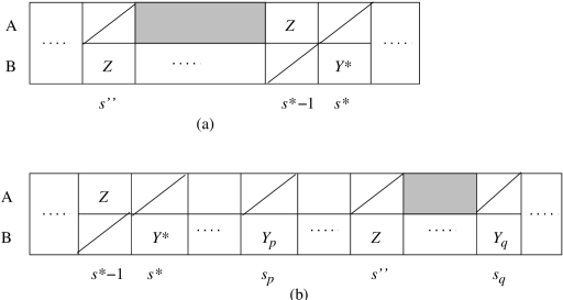
Figure 2: Positions of $Y_{i+1}$ and $Y_{p}$ in $A$ and $B$.

If $s^{\prime\prime}>s^{*}-1$, then let $s_{p}$ be the closest slot among $s_{0},s_{1},\ldots,s_{i}$ before $s^{\prime\prime}$. See Figure 2(b). Such slot must exist because $s^{*}$ is one such candidate. Then $w(Y_{p})\geq w(Z)$ or else $Z$ would have been accepted in slot $s_{p}$. Therefore, $w(A(\tilde{s}))\geq w(Y_{p})\geq w(Z)$ for every odd slot $\tilde{s}\in[s^{\prime\prime}+1..s_{q}-1]$. $\Box$

Lemma 4.5

In Step $i$.3, $B$ accepts $Z$ in a slot $s^{\prime\prime}$ where $s^{\prime\prime}<\min(s,s^{\prime})$.

Proof. First notice that $w(B(s+1))<w(Y)\leq w(Y_{i+1})$. Therefore, $s^{\prime\prime}<s$ or else $Z$ would have been a candidate for slot $s+1$.

Now we assume that $s^{\prime}<s$ and show that $s^{\prime\prime}<s^{\prime}$. We distinguish two cases.

Case i. $s^{\prime}$ is an odd slot. Let $U=A(s^{\prime})$. Let $s_{p}$ be the slot in $s_{0},\ldots,s_{i}$ that is closest to and before $s^{\prime}$ (which must exist because $s^{*}$ itself is a candidate). Note that $s^{*}-1$ must be before $s_{p}$ since it must be before $s^{\prime}$ and immediately before one of the $s_{j}$’s (in this case $s^{*}$), and $s_{p}$ is the latest such $s_{j}$’s before $s^{\prime}$.

We have $w(Z)>w(U)$ since a self charge is made instead of a downward charge. By Lemma 4.4(ii), $w(U)\geq w(Y_{p})$. Therefore $w(Z)>w(Y_{p})$. Hence $Z$ must be accepted before $Y_{p}$ in $B$ or else it can take $Y_{p}$’s place in $B$. By definition of $s_{p}$, $s_{p}<s^{\prime}$. Hence $s^{\prime\prime}<s^{\prime}$.

Case ii. $s^{\prime}$ is an even slot. Let $U=B(s^{\prime})$. Then $w(Z)>w(U)$ due to no downward charge in slot $s^{\prime}$. Thus $B$ must have accepted $Z$ before $s^{\prime}$, i.e., $s^{\prime\prime}<s^{\prime}$.

So in all cases $B$ accepts $Z$ at some slot $s^{\prime\prime}<\min(s,s^{\prime})$. $\Box$

Finally, the lemma below shows that two bad slots are paired with different good slots.

Lemma 4.6

All bad slots are paired with different good slots.

Proof. There are two possible places in our procedure where good slots can be identified: in Step $j$.1 or in Step $k$.2 for some $j$ and $k$. Call them substeps 1 and 2. Note that, for an odd bad slot, good slots identified in substep 1 are always when $B$ is accepting jobs, and good slot identified in substep 2 are always when $A$ is accepting jobs, and vice versa for even bad slots.

Consider two distinct bad slots $s=(X,Y)$ and $s^{\prime}=(X^{\prime},Y^{\prime})$. First, consider the case when $s$ and $s^{\prime}$ has different parity (odd or even slots). Then they can match with the same good slot only if one of them identifies it in substep 1 and the other in substep 2. However, a good slot in substep 1 must receive self-charge (this is how the $Y_{j}$’s are identified) while a good slot in substep 2 cannot receive a self charge (otherwise we would have moved on to some Step $i$.3 in the procedure). Thus it is impossible that a substep 1 good slot is also a substep 2 good slot.

Next, consider the case when $s$ and $s^{\prime}$ are of the same parity. Without loss of generality assume that they are both odd slots. To facilitate our discussion, we re-index the $Y_{j}$’s in the order they are identified. So we let $Y_{0},Y_{1},Y_{2},\ldots$ be the chain of $Y_{j}$’s associated with $s$ where $\{Y_{0},Y_{1}\}=\{X,Y\}$ and for $j\geq 2$, $Y_{j}$ is the job identified in step $(j-1)$.3. Similarly, we let $Y^{\prime}_{0},Y^{\prime}_{1},Y^{\prime}_{2}\ldots$ be the chain associated with $s^{\prime}$. We will show that no job appears in both chains. This proves the claim because for two bad slots of the same parity to be matched to the same good slot, they must both be identified in substep 1 or both in substep 2. But if the chains of $Y_{i}$’s associated with them are different, this is not possible.

To show the chains are distinct, we first show that $Y_{0},Y_{1},Y^{\prime}_{0}$ and $Y^{\prime}_{1}$ are all distinct. Recall that $\{X,Y\}=\{Y_{0},Y_{1}\}$ and $\{X^{\prime},Y^{\prime}\}=\{Y^{\prime}_{0},Y^{\prime}_{1}\}$. Clearly $X\neq Y,X^{\prime}\neq Y^{\prime},X\neq X^{\prime}$ and $Y\neq Y^{\prime}$. Thus we only need to show that $X\neq Y^{\prime}$ and $X^{\prime}\neq Y$. If this is not true, then either: (1) $Y$ is accepted in $A$ in a bad slot; or (2) $X$ in $OPT$ generates a backward charge. For (1), if $A^{-1}(Y)<A^{-1}(X)(=s)$, then $OPT(s+1)(=Y)$ would not make a backward charge to $s$; while if $A^{-1}(Y)>s$, then $A^{-1}(Y)$ cannot get a self charge and hence receives at most 1.5 units of charge. For (2), $OPT^{-1}(X)>OPT^{-1}(Y)$ due to the self charge to slot $s$, and by Lemma 4.3(i), $X$ must also be accepted in $B$ before $s$. Hence $X$ cannot generate a backward charge. Thus neither (1) nor (2) can be true.

We have now established that $Y_{0},Y_{1},Y^{\prime}_{0}$ and $Y^{\prime}_{1}$ are all different. It is also clear that $Y_{j}\neq Y_{k}$ and $Y^{\prime}_{j}\neq Y^{\prime}_{k}$ for any $j$ and $k$. Note that, if $Y_{j}=Y^{\prime}_{k}$, for some $j>1$ and $k>1$, then there must be some $j^{\prime}<j$ and $k^{\prime}<k$ such that $Y_{j^{\prime}}=Y^{\prime}_{k^{\prime}}$, because they are uniquely defined in such a way (in some substep 2). So the only remaining case to consider is $Y_{0}$ or $Y_{1}$ being the same as $Y^{\prime}_{j}$ for some $j>1$. Recall $Y_{0}$ and $Y_{1}$ are the $X$ and $Y$ of $s$. $Y^{\prime}_{j}$ cannot be $Y$ because by Lemma 4.5, both $A$ and $B$ accept $Y^{\prime}_{j}$ before $OPT$ does but $A$ accepts $Y$ after $OPT$. $Y^{\prime}_{j}$ cannot be $X$ because this would mean the job $B(s+1)$ is $Y^{\prime}_{k}$ for some $k<j$, so slot $s+1$ should receive a downward charge but this contradicts that $OPT(s+1)$ makes a backward charge to $s$ instead of a downward charge. $\Box$

5 Lower Bound for Equal Length Intervals

In this section, we show a lower bound of 2 for barely random algorithms for scheduling equal length intervals that choose between two deterministic algorithms, possibly with unequal probability.

Theorem 5.1

No barely random algorithm choosing between two deterministic algorithms for the online scheduling of equal length intervals has a competitive ratio better than $2$.

Let $ALG$ be a barely random algorithm that chooses between two deterministic algorithms $A$ and $B$ with probability $p$ and $q$ respectively such that $p+q=1$ and $0<p\leq q<1$. Let $\delta$ be an arbitrarily small positive constant less than 1. We will show that there is an input on which $OPT$ gains at least $2-\delta$ times of what $ALG$ gains.

We will be using sets of intervals similar to that in Woeginger [19]. More formally, let $\epsilon$ be an arbitrary positive real number and let $v,w$ be any pair of real numbers such that $0\leq v\leq w$. We define $SET(v,w,\epsilon)$ as a set of intervals of weight $v,v+\epsilon^{\prime},v+2\epsilon^{\prime},\dots,w$ (where $\epsilon^{\prime}$ is the largest number such that $\epsilon^{\prime}\leq\epsilon$ and $w-v$ is a multiple of $\epsilon^{\prime}$) and their relative arrival times are such that intervals of smaller weight come earlier and the last interval (i.e., the one that arrives last and has weight $w$) arrives before the first interval finishes. Thus, there is overlapping between any pair of intervals in the set. See Figure 3. This presents a difficulty for the online algorithm as it has to choose the right interval to process without knowledge of the future.

Figure 3: $SET(v,w,\epsilon)$. On the left is the actual set of intervals; the vertical arrow on the right is the notation we use to denote such a set.

To facilitate our discussion, we assume that all intervals have weight at least 1 throughout this section, except Section 5.3. If $I$ is an interval in $SET(v,w,\epsilon)$ and $w(I)>v$ (i.e., $I$ is not the earliest interval in the set), then $I^{-}$ denotes the interval that arrives just before $I$ in $SET(v,w,\epsilon)$. So, $w(I^{-})\geq w(I)-\epsilon$.

5.1 A Few Simple Cases

We first present a few simple situations in which $OPT$ can gain a lot compared with what $ALG$ can gain. The first lemma shows that an algorithm should not start an interval that is lighter than the current interval being processed by the other algorithm. The second lemma shows that it is not good to have $A$ processing an interval of equal or heavier weight than the interval currently being processed by $B$. Moreover, the two algorithms should avoid processing almost non-overlapping intervals as shown in the third lemma.

Lemma 5.1

Suppose at some moment, one of the algorithms (say $B$) is processing an interval $J$ from a set $S=SET(v,w,\epsilon)$ while the other algorithm ($A$) is processing another interval $I$, where $w(J)>v$, $w(I)\leq w(J)$ and $r(I)>r(J)$. (Note that here the interval $I$ cannot come from $S$.) Then $OPT$ gains at least $2-\epsilon$ of $ALG$’s gain on an input consisting of $S$, $I$ and some subsequently arrived intervals.

Proof. We illustrate the scenario in Figure 4. (There, the vertical line represents the set $S$ and the horizontal line labelled $J$ is one of the intervals in $S$. The horizontal line labelled $I$ arrives later than $J$ and has a smaller weight.) To defeat $ALG$, an interval $J^{\prime}$ with the same weight as $J$ is released between $d(J^{-})$ and $d(J)$ and no more intervals are released. (See Figure 4.) Then $OPT$ completes $J^{-}$ (which finishes just before $J^{\prime}$ starts) and $J^{\prime}$, gaining $w(J^{-})+w(J^{\prime})$ $\geq 2w(J)-\epsilon$ while $ALG$ gains at most $(p+q)w(J)=w(J)$ even if it aborts $I$ to start $J^{\prime}$. Since $w(J)\geq 1$, $\frac{2w(J)-\epsilon}{w(J)}\geq 2-\epsilon$. $\Box$

Figure 4: (Lemma 5.1) Starting a lighter interval later

Lemma 5.2

Suppose at some moment, algorithm $B$ is processing an interval $I$ from a set $S=SET(v,w,\epsilon)$ while $A$ is processing an interval $J$ from a set $S^{\prime}=SET(v^{\prime},w^{\prime},\epsilon^{\prime})$, where $w(I)>v$, $w(J)>v^{\prime}$, $w(I)\leq w(J)$ and $r(I)\leq r(J)$. (Note that $S$ and $S^{\prime}$ can be the same set; $I$ and $J$ can even be the same interval.) Then $OPT$ gains at least $2-\max\{\epsilon,\epsilon^{\prime}\}$ of $ALG$’s gain on an input consisting of $S$, $S^{\prime}$ and some subsequently arrived intervals.

Proof. An interval $J^{\prime}$ with the same weight as $J$ is released between $d(I^{-})$ and $d(I)$. See Figure 5. Clearly there is no point in algorithm $A$ aborting $J$ to start $J^{\prime}$. If algorithm $B$ continues with $I$, then no more intervals arrived. $OPT$ gains $w(I^{-})+w(J^{\prime})\geq w(I)+w(J)-\epsilon$ while $ALG$ gains $qw(I)+pw(J)$ $\leq(w(I)+w(J))/2$. Since $(w(I)+w(J))/2\geq 1$, we have $\frac{w(I)+w(J)-\epsilon}{(w(I)+w(J))/2}\geq 2-\epsilon$. If $B$ aborts $I$ and starts $J^{\prime}$, then using Lemma 5.1, we can see that $OPT$ gains at least $2-\epsilon^{\prime}$ of what $ALG$ gains on an input consisting of $S$, $S^{\prime}$ and the subsequently arrived intervals specified in Lemma 5.1. $\Box$

Figure 5: (Lemma 5.2) $A$ processing a heavier interval ($J$)

Lemma 5.3

Suppose at some moment, algorithm $A$ is processing an interval $I$ from a set $S=SET(v,w,\epsilon)$ while algorithm $B$ is processing an interval $J$ from another set $S^{\prime}=SET(v^{\prime},w^{\prime},\epsilon^{\prime})$, where $w(I)>v$, $w(J)>v^{\prime}$, $w(I)\leq w(J)$ and the intervals of $S^{\prime}$ arrive between $d(I^{-})$ and $d(I)$. Then $OPT$ gains at least $2-(\epsilon+\epsilon^{\prime})$ of $ALG$’s gain on an input consisting of $S$, $S^{\prime}$ and some subsequently arrived intervals. in the worst case.

Proof. An interval $J^{\prime}$ with the same weight as $J$ is released between $d(J^{-})$ and $d(J)$ and no more intervals are released. See Figure 6. OPT completes $I^{-}$ in $S$, $J^{-}$ in $S^{\prime}$ and $J^{\prime}$. So it gains $w(I^{-})+w(J^{-})+w(J^{\prime})$ $\geq w(I)+2w(J)-(\epsilon+\epsilon^{\prime})$. On the other hand, $A$ completes $I$ and then $J^{\prime}$ while $B$ completes $J$. Thus $ALG$ gains at most $p(w(I)+w(J))+qw(J)=pw(I)+w(J)$ $\leq(1/2)w(I)+w(J)$. Since $w(I)/2+w(J)\geq 1$, we have $\frac{w(I)+2w(J)-(\epsilon+\epsilon^{\prime})}{w(I)/2+w(J)}$ $\geq 2-(\epsilon+\epsilon^{\prime})$. $\Box$

Figure 6: (Lemma 5.3) $A$ and $B$ processing almost non-overlapping intervals

5.2 Constructing the Sequence of Intervals

Our lower bound proof takes a number of steps. In each step, the adversary will release some set of intervals $SET(\cdot,\cdot,\cdot)$ adaptively according to how $ALG$ reacts in the previous steps. In each step, the adversary forces $ALG$ not to finish any interval (and hence gain no value) while $OPT$ will gain some. Eventually, $OPT$ will accumulate at least $2-\delta$ times of what $ALG$ can gain no matter what $ALG$ does in the last step.

5.2.1 Step 1

Let $c=2-\delta/2$. The adversary releases $S_{1}=SET(v_{1},w_{1},\epsilon_{1})$ where $v_{1}$ is some positive real number at least one, $w_{1}=c(q/p)(4/\delta)v_{1}$ and $\epsilon_{1}=\delta/8$. Denote by $I_{1}$ and $J_{1}$, where $w(I_{1})\leq w(J_{1})$, the intervals chosen by $ALG$. We claim that

Lemma 5.4

Both algorithms $A$ and $B$ do not process the smallest-weight interval in $S_{1}$, i.e.,

(i)

$w(I_{1})>v_{1}$ and

(ii)

$w(J_{1})>v_{1}$.

Hence both $I_{1}^{-}$ and $J_{1}^{-}$ exist.

Proof. We first prove part (ii). By Lemma 5.2, we assume that $I_{1}$ is processed by $A$ and $J_{1}$ is processed by $B$. So, the expected gain by $ALG$ is $pw(I_{1})+qw(J_{1})$ $\leq w(J_{1})$. Then we deduce that $w(J_{1})>w_{1}/c$ or else the adversary stops, $OPT$ schedules the heaviest interval in $S_{1}$ (of weight $w_{1}$) so that it gains at least $c>2-\delta$ times the expected gain by $ALG$. Since $v_{1}=(p/q)(\delta/4)(w_{1}/c)$ $<w_{1}/c$, we have $w(J_{1})>v_{1}$.

To prove part (i), we assume to the contrary that $w(I_{1})=v_{1}$. Then an interval $J^{\prime}_{1}$ with the same weight as $J_{1}$ is released between $d(J_{1}^{-})$ and $d(J_{1})$. See Figure 7(a). $OPT$ can gain $w(J^{-}_{1})+w(J^{\prime}_{1})\geq 2w(J_{1})-\epsilon_{1}$ by executing $J^{-}_{1}$ in $S_{1}$ and then $J^{\prime}_{1}$. Upon finishing $I_{1}$, algorithm $A$ can go on to finish $J^{\prime}_{1}$. The expected gain of $ALG$ is at most $p(w(I_{1})+w(J^{\prime}_{1}))+qw(J_{1})$ $=pw(I_{1})+w(J_{1})$. Note that $v_{1}=(p/q)(\delta/4)(w_{1}/c)\leq(\delta/4)w(J_{1})$ and $pw(I_{1})=pv_{1}$ $<(\delta/4)w(J_{1})$. Thus $ALG$’s gain is at most $pw(I_{1})+w(J_{1})$ $\leq(1+\delta/4)w(J_{1})$. So $OPT$’s gain is more than $2-\delta$ times that of $ALG$’s. $\Box$

                  

Figure 7: Step 1. (left) Lemma 5.4, (right) Lemma 5.6

Lemma 5.5

$w(J_{1})<2w(I_{1})$.

We defer this to Section 5.3, where we prove that if $w(J_{1})\geq 2w(I_{1})$ then the adversary can force the competitive ratio to be at least $2-\delta$.

The adversary then releases a new set of intervals $S_{2}=SET(v_{2},w_{2},\epsilon_{2})$ such that all these intervals arrive between $d(I^{-}_{1})$ and $d(I_{1})$, where $v_{2}=w(I_{1})$, $w_{2}=\max\{c(pw(I_{1})+qw(J_{1}))-w(I_{1}),v_{2}\}$ and $\epsilon_{2}=\epsilon_{1}/2$. See Figure 7(b).

Lemma 5.6

Upon the release of $S_{2}$, both $A$ and $B$ must abort their current intervals in $S_{1}$ and start some intervals $I_{2}$ and $J_{2}$ respectively in $S_{2}$. Moreover, $v_{2}<w(I_{2})<w(J_{2})$.

Proof. If $ALG$ ignores $S_{2}$ and continues with both $I_{1}$ and $J_{1}$, then the expected gain of $ALG$ is $pw(I_{1})+qw(J_{1})$ while $OPT$ can complete $I^{-}_{1}$ and the last interval in $S_{2}$, gaining $w(I^{-}_{1})+w_{2}$ $\geq c(pw(I_{1})+qw(J_{1}))-\epsilon_{1}$ $=(2-\frac{\delta}{2})(pw(I_{1})+qw(J_{1}))-\frac{\delta}{8}$ $\geq(2-\delta)(pw(I_{1})+qw(J_{1}))$.

Suppose algorithm $B$ aborts $J_{1}$ and starts some $J_{2}$ in $S_{2}$ while algorithm $A$ continues to process $I_{1}$. Then by Lemma 5.3, $ALG$ loses. Suppose algorithm $B$ continues with $J_{1}$ but $A$ aborts $I_{1}$ to start some $I_{2}$ in $S_{2}$. By Lemma 5.2, it must be the case that $w(I_{2})<w(J_{1})$. But then by Lemma 5.1, $ALG$ loses too.

Based on the above discussion, the only remaining sensible response for $ALG$ is to abort both $I_{1}$ and $J_{1}$ and start some $I_{2}$ and $J_{2}$ in $S_{2}$. By Lemma 5.2, we can further assume that $w(I_{2})<w(J_{2})$. Moreover, we claim that $w(I_{2})>v_{2}$. Otherwise, $ALG$ is effectively aborting only $J_{1}$ but not $I_{1}$. Then the construction of inputs given in Lemma 5.3 can be used to defeat $ALG$. $\Box$

This finishes our discussion on Step 1 and we now proceed to Step 2.

5.2.2 Step $i$

In general, at the beginning of Step $i\geq 2$, we have the following situation: $OPT$ has gained $w(I_{1}^{-})+w(I_{2}^{-})+\cdots w(I_{i-1}^{-})$ while $ALG$ has not gained anything yet. Moreover, $A$ and $B$ of $ALG$ are respectively executing $I_{i}$ and $J_{i}$ in $S_{i}=SET(v_{i},w_{i},\epsilon_{i})$ where $v_{i}=w(I_{i-1})$, $w_{i}=\max\{c(pw(I_{i-1})+qw(J_{i-1}))-\sum_{j=1}^{i-1}w(I_{j}),v_{i}\}$, $\epsilon_{i}=\epsilon_{1}/2^{i-1}$ and $v_{i}<w(I_{i})<w(J_{i})$. We go through a similar analysis to that in Step 1.

First, as in Lemma 5.5, we have $w(J_{i})<2w(I_{i})$ (the case $w(J_{i})\geq 2w(I_{i})$ is handled in the next subsection). Next, the adversary releases $S_{i+1}=SET(v_{i+1},w_{i+1},\epsilon_{i+1})$ in the period between $d(I^{-}_{i})$ and $d(I_{i})$ where $v_{i+1}=w(I_{i})$, $w_{i+1}=\max\{c(pw(I_{i})+qw(J_{i}))-\sum_{j=1}^{i}w(I_{j}),v_{i+1}\}$ and $\epsilon_{i+1}=\epsilon_{1}/2^{i}$. See Figure 8.

Figure 8: Step $i$

Similar to Lemma 5.6, we can prove that

Lemma 5.7

Upon the release of $S_{i+1}$, both $A$ and $B$ must abort their current intervals in $S_{i}$ and start some intervals $I_{i+1}$ and $J_{i+1}$ respectively in $S_{i+1}$. Moreover, $v_{i+1}<w(I_{i+1})<w(J_{i+1})$.

Proof. $ALG$ cannot continue with both $I_{i}$ and $J_{i}$. Otherwise, $OPT$ schedules (after finishing $I_{1}^{-},\ldots,I_{i-1}^{-}$) $I_{i}^{-}$ and then the last interval of $S_{i+1}$, thus gaining at least

$$\sum_{j=1}^{i}w(I_{j}^{-})+c(pw(I_{i})+qw(J_{i}))-\sum_{j=1}^{i}w(I_{j})$$

$$\geq c(pw(I_{i})+qw(J_{i}))-\sum_{j=1}^{i}\epsilon_{j}$$

$$> (2-\frac{\delta}{2})(pw(I_{i})+qw(J_{i}))-2\epsilon_{1}$$

$$\geq (2-\delta)(pw(I_{i})+qw(J_{i})).$$

Suppose $B$ aborts $J_{i}$ in order to start some $J_{i+1}$ in $S_{i+1}$ while $A$ continues with $I_{i}$. Then by Lemma 5.3, $ALG$ loses. Suppose $B$ continues with $J_{i}$ while $A$ aborts $I_{i}$ to start $I_{i+1}$. By Lemma 5.2, we have that $w(I_{i+1})<w(J_{i})$. Then by Lemma 5.1, $ALG$ loses too.

Based on the above reasoning, we conclude that $ALG$ has to abort both $I_{i}$ and $J_{i}$ and start some $I_{i+1}$ and $J_{i+1}$ in $S_{i+1}$. By Lemma 5.2, we can assume that $w(I_{i+1})<w(J_{i+1})$. We can also argue that $w(I_{i+1})>v_{i+1}$ in the same way as proving $w(I_{2})>v_{2}$ in Step 1. $\Box$

We now proceed to Step $i+1$. Note that $OPT$ has already gained $w(I_{1}^{-})+\cdots+w(I_{i}^{-})$ while $ALG$ still has not gained anything. We will make use of Lemma 4.3 of Woeginger [19]:

Lemma 5.8

(Woeginger [19]). For $2<d<4$, any strictly increasing sequence of positive numbers $\langle a_{1},a_{2},\ldots\rangle$ fulfilling the inequality

$$a_{i+1}\leq da_{i}-\sum_{j=1}^{i}a_{j}$$

for every $i\geq 1$ must be finite.

Consider the sequence $\langle w(I_{1}),w(I_{2}),\ldots\rangle$. It is strictly increasing since $w(I_{i+1})>v_{i+1}=w(I_{i})$ for all $i$. Moreover, recall that $w_{i+1}$ is set to be the maximum of either $c(pw(I_{i})+qw(J_{i}))-\sum_{j=1}^{i}w(I_{j})$ or $v_{i+1}$. If $c(pw(I_{i})+qw(J_{i}))-\sum_{j=1}^{i}w(I_{j})>v_{i+1}$ for all $i\geq 1$, then we have $w(I_{i+1})\leq w_{i+1}$ $=\max\{c(pw(I_{i})+qw(J_{i}))-\sum_{j=1}^{i}w(I_{j}),v_{i+1}\}$ $=c(pw(I_{i})+qw(J_{i}))-\sum_{j=1}^{i}w(I_{j})$ $\leq cw(J_{i})-\sum_{j=1}^{i}w(I_{j})$ $<(4-\delta)w(I_{i})-\sum_{j=1}^{i}w(I_{j})$ (since $w(J_{i})<2w(I_{i})$) for all $i$. The existence of such an infinite sequence contradicts Lemma 5.8. So, eventually, there is a finite $k$ such that $c(pw(I_{k})+qw(J_{k}))-\sum_{j=1}^{k}w(I_{j})\leq v_{k+1}$ and hence we set $w_{k+1}=v_{k+1}$ and the next (and final) set $S_{k+1}$ consists of a single interval of weight $w_{k+1}$ ($=w(I_{k})$).

In that situation, it makes no difference whether $A$ or $B$ of $ALG$ aborts $I_{k}$ or $J_{k}$ to start the interval in $S_{k+1}$ since it has weight equal to $w(I_{k})$. Its expected gain is still at most $pw(I_{k})+qw(J_{k})$. On the other hand, $OPT$ schedules the interval of $S_{k+1}$ and gains in total $w(I_{1}^{-})+\cdots+w(I_{k}^{-})+w_{k+1}$ $\geq c(pw(I_{k})+qw(J_{k}))-2\epsilon_{1}$ which is at least $2-\delta$ times of $ALG$’s gain.

5.3 The Case of $w(J_{i})\geq 2w(I_{i})$

We now consider the case where in some Step $i\geq 1$, $w(J_{i})\geq 2w(I_{i})$. We will show how the adversary forces $ALG$ to lose the game, i.e., $OPT$ will gain at least $2-\delta$ of what $ALG$ can on $S_{i}$ and a set of subsequently arrived intervals. For simplicity, we drop the subscript $i$ in $I_{i}$, $J_{i}$, and $\epsilon_{i}$ in the following discussion.

Intuitively, when $w(J)$ is relatively large compared with $w(I)$, we can afford to let algorithm $A$ finish the interval $I$ and gain $pw(I)$, which is relatively small. Therefore, a set $S_{u}=SET(0,uw(J),\epsilon)$ is released between $d(J^{-})$ and $d(J)$, where $u\geq 1$ is some parameter to be determined as a function of $p$. This allows algorithm $A$ to finish $I$ and then start some job in this new set $S_{u}$. On the other hand, algorithm $B$ has to decide whether to abort or continue with the current interval $J$. We will show that there is a choice of $u$ such that no matter what $B$ does, $OPT$ can gain at least $2-\delta$ of what $ALG$ gains.

Case 1: Algorithm $B$ continues with $J$.

Then $ALG$ gains at most $p(w(I)+uw(J))+qw(J)$ while $OPT$ can gain $w(J^{-})+uw(J)$. Therefore, the ratio of the gain by $OPT$ to that of $ALG$ on $S$ and $S_{u}$ is at least

$$\frac{w(J^{-})+uw(J)}{p(w(I)+uw(J))+qw(J)} \geq \frac{(1+u)w(J)-\epsilon}{p(w(J)/2+uw(J))+(1-p)w(J)}$$

$$\geq \frac{1+u-\epsilon/w(J)}{p(1/2+u)+1-p}$$

where the first inequality makes use of the condition that $w(I)\leq w(J)/2$. This ratio is at least $2-\delta$ provided

$$1+u-\frac{\epsilon}{w(J)} \geq (2-\delta)(1-\frac{p}{2}+pu)$$

$$= (2-\delta-p+\frac{p\delta}{2})+(2p-p\delta)u.$$

After simplifying using $\epsilon/w(J)\leq\epsilon<\delta$, this condition is satisfied by having

$$u \geq \frac{1-p+p\delta/2}{1-2p+p\delta}.$$ (2)

Case 2: Algorithm $B$ aborts $J$.

Then algorithms $A$ and $B$ can start some intervals $I^{\prime}$ and $J^{\prime}$ in $S_{u}=SET(0,uw(J),\epsilon)$. By Lemma 5.2, we can assume that $w(I^{\prime})\leq w(J^{\prime})$. Then another interval $J^{\prime\prime}$ with the same weight as $J^{\prime}$ is released between $d((I^{\prime})^{-})$ and $d(I^{\prime})$.

If $ALG$ aborts $I^{\prime}$ to start $J^{\prime\prime}$, by Lemma 5.1, $OPT$ gains at least $2-\epsilon$ of $ALG$’s gain on $S_{u}$ and a set of subsequently arrived intervals. Also, on the set of intervals $S=SET(v,w,\epsilon)$, $ALG$ gains $pw(I)\leq w(I)/2$ while $OPT$ gains at least $w(J)-\epsilon$ $\geq w(I)-\epsilon$. So $ALG$ loses.

On the other hand, if $ALG$ does not abort $I^{\prime}$, then its expected gain is at most $p(w(I)+w(I^{\prime}))+qw(J^{\prime})$ $\leq p(w(J)/2+w(I^{\prime}))+(1-p)w(J^{\prime})$. $OPT$ will complete $J^{-}$ in $S$, $(I^{\prime})^{-}$ in $S_{u}$ and then $J^{\prime\prime}$. (Note that if $I^{\prime}$ is the first interval with weight 0 in $S_{u}$, then we set $(I^{\prime})^{-}$ to be of weight 0 too.) The ratio of the gain by $OPT$ to that of $ALG$ on $S$, $S_{u}$ and $J^{\prime\prime}$ is at least

$$\frac{(w(J)-\epsilon)+(w(I^{\prime})-\epsilon)+w(J^{\prime\prime})}{p(w(J)/2+w(I^{\prime}))+(1-p)w(J^{\prime})}=\frac{w(I^{\prime})+w(J)+w(J^{\prime})-2\epsilon}{pw(I^{\prime})+pw(J)/2+(1-p)w(J^{\prime})}.$$

Since $1/p\geq 2>2-\delta$, it suffices to show that

$$f = \frac{w(J)+w(J^{\prime})-2\epsilon}{pw(J)/2+(1-p)w(J^{\prime})}$$

is at least $2-\delta$. Furthermore, $1/(p/2)\geq 2$ and $\frac{1-2\epsilon/w(J^{\prime})}{1-p}$ $<\frac{1}{1-p}\leq 2$. Therefore, the fraction $f$, as a function of $w(J^{\prime})$, is minimized when $w(J^{\prime})$ is maximized. That means,

$$f \geq \frac{w(J)+uw(J)-2\epsilon}{pw(J)/2+(1-p)uw(J)}$$

$$\geq \frac{1+u-2\epsilon}{p/2-pu+u}.$$

Observe that $\frac{p}{2}-pu+u$ $\geq\frac{p}{2}-p+1$ $\geq 1-\frac{p}{2}$ $>\frac{1}{2}$ using $u\geq 1$ and $p\leq 1/2$. Thus $\frac{2\epsilon}{p/2-pu+u}\leq\frac{\delta}{2}$ because $\epsilon\leq\delta/8$. Hence to show that $f\geq 2-\delta$, it suffices to show that $\frac{1+u}{p/2-pu+u}\geq 2-\frac{\delta}{2}$. This condition is satisfied provided

$$1+u \geq (2-\frac{\delta}{2})(\frac{p}{2}-pu+u)$$

$$= (p-\frac{p\delta}{4})+(2-2p+\frac{p\delta}{2}-\frac{\delta}{2})u.$$

or

$$(1-2p+\frac{p\delta}{2}-\frac{\delta}{2})u\leq 1-p+\frac{p\delta}{4}.$$

This is satisfied if

$$(1-2p+\frac{p\delta}{2})u\leq 1-p+\frac{p\delta}{4},$$

i.e.,

$$u \leq \frac{1-p+p\delta/4}{1-2p+p\delta/2}.$$ (3)

By setting

$$u = \frac{1-p+p\delta/4}{1-2p+p\delta/2},$$

both ineq. (1) and ineq. (2) are satsified. This completes the proof for the case of $w(J_{i})\geq 2w(I_{i})$.

6 Conclusion

In this paper, we designed 2-competitive barely random algorithms for various versions of preemptive scheduling of intervals. They are surprisingly simple and yet improved upon previous best results. Based on the same approach, we designed a 3-competitive algorithm for the preemptive (with restart) scheduling of equal length jobs. This is the first randomized algorithm for this problem. Finally, we gave a 2 lower bound for barely random algorithms that choose between two deterministic algorithms, possibly with unequal probability.

An obvious open problem is to close the gap between the upper and lower bounds for randomized preemptive scheduling of intervals in the various cases. We conjecture that the true competitive ratio is 2. Also, it is interesting to prove a randomized lower bound for the related problem of job scheduling with restart.

References

- [1] S. Albers. On randomized online scheduling. In Proc. 34th ACM Symposium on Theory of Computing, 134–143, 2002.
- [2] B. Awerbuch, Y. Bartal, A. Fiat, and A. Rosen. Competitive non-preemptive call control. In Proc. 5th ACM-SIAM Symposium on Discrete Algorithms, 312–320, 1994.
- [3] S. Baruah, G. Koren, D. Mao, B. Mishra, A. Raghunathan, L. Rosier, D. Shasha, and F. Wang. On the competitiveness of on-line real-time task scheduling. Real-Time Systems, 4:125–144, 1992.
- [4] K. P. Bogart and D. B. West. A short proof that ‘Proper = Unit’. Discrete Mathematics, 201:21–23, 1999.
- [5] A. Borodin and R. El-Yaniv. Online Computation and Competitive Analysis. Cambridge University Press, New York, 1998.
- [6] R. Canetti and S. Irani. Bounding the power of preemption in randomized scheduling. SIAM Journal on Computing, 27(4):993–1015, 1998.
- [7] F. Y. L. Chin, M. Chrobak, S. P. Y. Fung, W. Jawor, J. Sgall and T. Tichý. Online competitive algorithms for maximizing weighted throughput of unit jobs. Journal of Discrete Algorithms, 4(2):255–276, 2006.
- [8] F. Y. L. Chin and S. P. Y. Fung. Online scheduling with partial job values: does timesharing or randomization help? Algorithmica, 37(3):149–164, 2003.
- [9] M. Chrobak, W. Jawor, J. Sgall and T. Tichý. Online scheduling of equal-length jobs: randomization and restarts help. SIAM Journal on Computing 36(6):1709–1728, 2007.
- [10] M. Englert and M. Westermann. Considering suppressed packets improves buffer management in QoS switches. In Proc. 18th ACM-SIAM Symposium on Discrete Algorithms, 209–218, 2007.
- [11] L. Epstein and A. Levin. Improved randomized results for the interval selection problem. Theoretical Computer Science, 411(34-36):3129–3135, 2010.
- [12] S. P. Y. Fung, C. K. Poon and F. Zheng, Online interval scheduling: randomized and multiprocessor cases. In Proc. 13th International Computing and Combinatorics Conference, LNCS 4598, 176–186, 2007.
- [13] J.-H. Kim and K.-Y. Chwa. Scheduling broadcasts with deadlines. Theoretical Computer Science, 325(3):479–488, 2004.
- [14] G. Koren and D. Shasha. : An optimal on-line scheduling algorithm for overloaded uniprocessor real-time systems. SIAM Journal on Computing, 24:318–339, 1995.
- [15] F. Li, J. Sethuraman and C. Stein. An optimal online algorithm for packet scheduling with agreeable deadlines. In Proceedings of 16th ACM-SIAM Symposium on Discrete Algorithms, pages 801–802, 2005.
- [16] H. Miyazawa and T. Erlebach. An improved randomized on-line algorithm for a weighted interval selection problem. Journal of Scheduling, 7(4):293–311, 2004.
- [17] S. S. Seiden. Randomized online interval scheduling. Operations Research Letters, 22(4–5):171–177, 1998.
- [18] H.-F. Ting. A near optimal scheduler for on-demand data broadcasts. In Proc. 6th Italian Conference on Algorithms and Complexity, LNCS 3998, 163–174, 2006.
- [19] G. J. Woeginger. On-line scheduling of jobs with fixed start and end times. Theoretical Computer Science, 130(1):5–16, 1994.
- [20] F. Zheng, S. P. Y. Fung, W.-T. Chan, F. Y. L. Chin, C. K. Poon, and P. W. H. Wong. Improved on-line broadcast scheduling with deadlines. In Proc. 12th International Computing and Combinatorics Conference, LNCS 4112, 320–329, 2006.