Non-sparse Linear Representations for Visual Tracking
with Online Reservoir Metric Learning

Abstract

Most sparse linear representation-based trackers need to solve a computationally expensive $\ell_{1}$-regularized optimization problem. To address this problem, we propose a visual tracker based on non-sparse linear representations, which admit an efficient closed-form solution without sacrificing accuracy. Moreover, in order to capture the correlation information between different feature dimensions, we learn a Mahalanobis distance metric in an online fashion and incorporate the learned metric into the optimization problem for obtaining the linear representation. We show that online metric learning using proximity comparison significantly improves the robustness of the tracking, especially on those sequences exhibiting drastic appearance changes. Furthermore, in order to prevent the unbounded growth in the number of training samples for the metric learning, we design a time-weighted reservoir sampling method to maintain and update limited-sized foreground and background sample buffers for balancing sample diversity and adaptability. Experimental results on challenging videos demonstrate the effectiveness and robustness of the proposed tracker.

1 Introduction

Robust visual tracking is an important problem in computer vision. In recent years, steady improvements have been made to the speed, accuracy and robustness of tracking techniques. A crucial factor in many of these improvements has been the construction and optimization of object appearance models (e.g., [1, 2, 3, 4, 5, 6, 7, 8, 9]). Among these models, the linear representation, in which the object is represented as a linear combination of basis samples, has proved to be a simple yet effective choice. For example, Mei and Ling [2] propose a tracker based on a sparse linear representation which solves an $\ell_{1}$-regularized optimization problem. With the sparsity constraint, this tracker obtains a sparse regression solution that can adaptively select a small number of relevant templates to optimally approximate the given test samples. The drawback is its expensive computation due to the need of solving an $\ell_{1}$-norm convex problem. To speed up the tracking, Li et al. [4] propose to approximately solve the sparsity optimization problem using orthogonal matching pursuit (OMP). Recently, research has revealed that the $\ell_{1}$-norm induced sparsity does not in general help improve the accuracy of image classification; and non-sparse representation based methods are typically orders of magnitudes faster than the sparse representation based ones with competitive and sometimes even better accuracy [10, 11, 12].

Inspired by these findings, here we propose a non-sparse linear representation based visual tracker. The proposed tracker can be implemented by solving a least-square problem, which admits an extremely simple and efficient closed-form solution. To date, linear representation based trackers [2, 4] have built linear regressors that are defined on independent feature dimensions (mutually independent raw pixels in both [2] and [4]). In other words, the correlation information between different feature dimensions is not exploited. We argue that this correlation information is important in tracking. To address this problem, we learn a Mahalanobis distance metric and incorporate it into the optimization of the linear representation.

Metric learning has emerged as a useful tool for many applications. For example, in [13, 14], a Mahalanobis distance metric is learned using positive semidefinite programming. Discriminative metric learning has also been successfully applied to visual tracking [15, 16]. These works learn a distance metric mainly for object matching across adjacent frames, and the tracking is not carried out in the framework of linear representations. In this work, we learn a distance metric using proximity comparison for linear representation based tracking. The learning strategy is adapted from the online metric learning for image retrieval of Chechik et al. [17]. There, it has been shown that the online learning procedure is efficient and capable for large-scale learning. Nevertheless, it is not designed for dealing with time-varying data stream such as in real-time visual tracking.

Visual tracking is a time-varying process which deals with a dynamic stream data in an online manner. Due to memory limit, it is often impractical for trackers to store all the stream data. Furthermore, visual tracking in the current frame usually relies more on recently received samples than old samples due to its temporal coherence property. Therefore, it is necessary for trackers to maintain and update limited-sized data buffers for balancing between sample diversity and adaptability. To address this issue, we propose to use reservoir sampling [18, 19] for sequential random sampling. The conventional reservoir sampling in [18, 19] can only accomplish the task of uniform random sampling, which ignores the importance variance among samples. We therefore need a time-weighted reservoir sampling.

In summary, we propose a robust tracker that is based on metric-weighted linear representations and time-weighted reservoir sampling. Our main contributions are as follows.

1. We propose an online discriminative linear representation for visual tracking. The metric-weighted least-square optimization problem admits a closed-form solution, which significantly improves tracking efficiency. We also demonstrate that, with the emergence of new data, the closed-form solution can be efficiently updated by a sequence of simple matrix operations.

2. To further improve the discriminative capability of the linear representation for distinguishing foreground and background, we present an online Mahalanobis distance metric learning method and incorporate the learned metric into the optimization problem for obtaining a discriminative linear representation. The learned metric can effectively capture the correlation information between different feature dimensions. Such correlation information plays an important role in robust object/non-object classification.

3. To allow for real-time applications, we design a time-weighted reservoir sampling method to maintain and update limited-sized sample buffers for balancing between sample diversity and adaptability in the metric learning procedure. With the theory of [20, 21], larger weights are assigned to those recently received samples, which is particularly important for tracking. To our knowledge, it is the first time that reservoir sampling is used in an online metric learning setting that is tailored for robust visual tracking.

2 The proposed visual tracker

In this section, we describe the novel aspects of the proposed visual tracker:

1. Object state estimation. This is implemented by an online metric-weighted optimization, as described in Section 2.1;

2. Metric update using the online metric-weighted optimization in response to changing foreground and background, as described in Section 2.2;

3. Sample update used for object representation based on reservoir sampling, as described in Section 2.3.

2.1 Online metric-weighted linear representation

To effectively characterize dynamic appearance variations during tracking, an object is associated with an appearance subspace spanned by a set of basis samples, which encode the distribution of the object appearance. Therefore, the problem of visual tracking is converted to that of linear representation and reconstruction. As a result, the sample-to-subspace distance (e.g., linear reconstruction error) can be used for evaluating the likelihood of a test sample belonging to the object appearance. However, the conventional linear representations (e.g., used in [2, 4]) ignore the correlation information between feature dimensions. Due to the influence of complicated appearance variations, the correlation across feature dimensions usually differs greatly during tracking. In order to address this problem, we propose a metric-weighted linear representation based on solving a metric-weighted optimization problem under a learned distance metric. Consequently, the proposed linear representation is capable of capturing the varying correlation information between feature dimensions.

More specifically, given a set of basis samples $\mathbf{P}=(\mathbf{p_{i}})_{i=1}^{N}\in\mathcal{R}^{d\times N}$ and a test sample $\mathbf{y}\in\mathcal{R}^{d\times 1}$, we aim to discover a linear combination of $\mathbf{P}$ to optimally approximate the test sample $\mathbf{y}$ by solving the following optimization problem:

$$\underset{\mathbf{x}}{\min}\thinspace g(\mathbf{x};\mathbf{M},\mathbf{P},\mathbf{y})=\underset{\mathbf{x}}{\min}\thinspace(\mathbf{y}-\mathbf{P}\mathbf{x})^{T}\mathbf{M}(\mathbf{y}-\mathbf{P}\mathbf{x}),\vspace{-0.2cm}$$ (1)

where $\mathbf{x}\in\mathcal{R}^{N\times 1}$ and $\mathbf{M}$ is a symmetric distance metric matrix. The optimization problem (1) is a weighted linear regression problem whose analytical solution can be directly computed as:

$$\mathbf{x}^{\ast}=(\mathbf{P}^{T}\mathbf{M}\mathbf{P})^{-1}\mathbf{P}^{T}\mathbf{M}\mathbf{y}.\vspace{-0.2cm}$$ (2)

If $\mathbf{P}^{T}\mathbf{M}\mathbf{P}$ is a singular matrix, we directly use its pseudoinverse to compute $\mathbf{x}^{\ast}$. The main computational time of Equ. (2) is spent on the calculation of $(\mathbf{P}^{T}\mathbf{M}\mathbf{P})^{-1}$. For computational efficiency, we need to incrementally or decrementally update the inverse when $\mathbf{P}$ is expanded or reduced with one column under the same metric $\mathbf{M}$. Let $\mathbf{P_{n}}=(\mathbf{P}\thickspace\Delta\mathbf{p})$ denote the expanded matrix of $\mathbf{P}$. Clearly, the following relation holds:

$$(\mathbf{P_{n}})^{T}\mathbf{M}\mathbf{P_{n}}=\left(\begin{matrix}\mathbf{P}^{T}\mathbf{M}\mathbf{P}&\mathbf{P}^{T}\mathbf{M}\Delta\mathbf{p}\\ (\Delta\mathbf{p})^{T}\mathbf{M}\mathbf{P}&(\Delta\mathbf{p})^{T}\mathbf{M}\Delta\mathbf{p}\end{matrix}\right).$$

For simplicity, let $\mathbf{H}=(\mathbf{P}^{T}\mathbf{M}\mathbf{P})^{-1}$, $\mathbf{c}=\mathbf{P}^{T}\mathbf{M}\Delta\mathbf{p}$, and $r=(\Delta\mathbf{p})^{T}\mathbf{M}\Delta\mathbf{p}$. Since $\mathbf{M}$ is a symmetric matrix, $\mathbf{c}^{T}=(\Delta\mathbf{p})^{T}\mathbf{M}\mathbf{P}$. According to the theory of matrix computation [22], the corresponding inverse of $(\mathbf{P_{n}})^{T}\mathbf{M}\mathbf{P_{n}}$ can be computed as:

$$((\mathbf{P_{n}})^{T}\mathbf{M}\mathbf{P_{n}})^{-1}=\left(\begin{matrix}\mathbf{H}+\frac{\mathbf{H}\mathbf{c}\mathbf{c}^{T}\mathbf{H}}{r-\mathbf{c}^{T}\mathbf{H}\mathbf{c}}&-\frac{\mathbf{H}\mathbf{c}}{r-\mathbf{c}^{T}\mathbf{H}\mathbf{c}}\\ -\frac{\mathbf{c}^{T}\mathbf{H}}{r-\mathbf{c}^{T}\mathbf{H}\mathbf{c}}&\frac{1}{r-\mathbf{c}^{T}\mathbf{H}\mathbf{c}}\end{matrix}\right).$$ (3)

Similarly, let $\mathbf{P_{o}}$ denote the reduced matrix of $\mathbf{P}$ after removing the $i$-th column such that $1\leq i\leq N$. Based on [22], the corresponding inverse of $(\mathbf{P_{o}})^{T}\mathbf{M}\mathbf{P_{o}}$ can be computed as:

$$((\mathbf{P_{o}})^{T}\mathbf{M}\mathbf{P_{o}})^{-1}=\mathbf{H}(\mathcal{I}_{i},\mathcal{I}_{i})-\frac{\mathbf{H}(\mathcal{I}_{i},i)\mathbf{H}(i,\mathcal{I}_{i})}{\mathbf{H}(i,i)},\\ \vspace{-0.082cm}$$ (4)

where $\mathcal{I}_{i}=\{1,2,\ldots,N\}\backslash{\{i\}}$ stands for the index set except $i$. For adapting to object appearance changes, it is necessary for trackers to replace an old sample from the sample buffer with a new sample. In essence, the replacement operation can be decomposed into two stages: 1) old sample removal; and 2) new sample arrival. As a matter of fact, 1) and 2) correspond to the decremental and incremental cases, respectively. Given $\mathbf{H}=(\mathbf{P}^{T}\mathbf{M}\mathbf{P})^{-1}$, we first compute the decremental inverse $((\mathbf{P_{o}})^{T}\mathbf{M}\mathbf{P_{o}})^{-1}$ according to Equ. (4), and then calculate the incremental inverse $((\mathbf{P_{o}}\thickspace\Delta\mathbf{p})^{T}\mathbf{M}(\mathbf{P_{o}}\thickspace\Delta\mathbf{p}))^{-1}$ using Equ. (3). For notational simplicity, we let $\mathbf{P^{\prime}}=(\mathbf{P_{o}}\thickspace\Delta\mathbf{p})$, $\mathbf{H_{o}}=((\mathbf{P_{o}})^{T}\mathbf{M}\mathbf{P_{o}})^{-1}$, $\mathbf{c_{o}}=(\mathbf{P_{o}})^{T}\mathbf{M}\Delta\mathbf{p}$, and $r=(\Delta\mathbf{p})^{T}\mathbf{M}\Delta\mathbf{p}$. Based on Equ. (3), $((\mathbf{P^{\prime}})^{T}\mathbf{M}\mathbf{P^{\prime}})^{-1}$ can be computed as:

$$((\mathbf{P^{\prime}})^{T}\mathbf{M}\mathbf{P^{\prime}})^{-1}=\left(\begin{matrix}\mathbf{H_{o}}+\frac{\mathbf{H_{o}}\mathbf{c_{o}}\mathbf{c_{o}}^{T}\mathbf{H_{o}}}{r-\mathbf{c_{o}}^{T}\mathbf{H_{o}}\mathbf{c_{o}}}&-\frac{\mathbf{H_{o}}\mathbf{c_{o}}}{r-\mathbf{c_{o}}^{T}\mathbf{H_{o}}\mathbf{c_{o}}}\\ -\frac{\mathbf{c_{o}}^{T}\mathbf{H_{o}}}{r-\mathbf{c_{o}}^{T}\mathbf{H_{o}}\mathbf{c_{o}}}&\frac{1}{r-\mathbf{c_{o}}^{T}\mathbf{H_{o}}\mathbf{c_{o}}}\end{matrix}\right)\vspace{-0.082cm}$$ (5)

Furthermore, when updated according to Algorithm 2, $\mathbf{M}$ is modified as a rank-one addition such that $\mathbf{M}\longleftarrow\mathbf{M}+\eta(\mathbf{a}_{-}\mathbf{a}_{-}^{T}-\mathbf{a}_{+}\mathbf{a}_{+}^{T})$ where $\mathbf{a}_{+}=\mathbf{p}-\mathbf{p}^{+}$ and $\mathbf{a}_{-}=\mathbf{p}-\mathbf{p}^{-}$ are two vectors (defined in Equ. (14)) for triplet construction, and $\eta$ is a step-size factor (defined in Equ. (21)). As a result, the original $\mathbf{P}^{T}\mathbf{M}\mathbf{P}$ becomes $\mathbf{P}^{T}\mathbf{M}\mathbf{P}+(\eta\mathbf{P}^{T}\mathbf{a}_{-})(\mathbf{P}^{T}\mathbf{a}_{-})^{T}+(-\eta\mathbf{P}^{T}\mathbf{a}_{+})(\mathbf{P}^{T}\mathbf{a}_{+})^{T}$. When $\mathbf{M}$ is modified by a rank-one addition, the inverse of $\mathbf{P}^{T}\mathbf{M}\mathbf{P}$ can be easily updated according to the theory of [23, 24]:

$$(\mathbf{J}+\mathbf{u}\mathbf{v}^{T})^{-1}=\mathbf{J}^{-1}-\frac{\mathbf{J}^{-1}\mathbf{u}\mathbf{v}^{T}\mathbf{J}^{-1}}{1+\mathbf{v}^{T}\mathbf{J}^{-1}\mathbf{u}}.\vspace{-0.02cm}$$ (6)

Here, $\mathbf{J}=\mathbf{P}^{T}\mathbf{M}\mathbf{P}$, $\mathbf{u}=\eta\mathbf{P}^{T}\mathbf{a}_{-}$ (or $\mathbf{u}=-\eta\mathbf{P}^{T}\mathbf{a}_{+}$), and $\mathbf{v}=\mathbf{P}^{T}\mathbf{a}_{-}$ (or $\mathbf{v}=\mathbf{P}^{T}\mathbf{a}_{+}$). The complete procedure of online linear optimization under the metric $\mathbf{M}$ is summarized in Algorithm 1.

Algorithm 1 Metric-weighted linear representation

Input:

The current distance metric matrix $\mathbf{M}$, the basis samples $\mathbf{P}=(\mathbf{p_{i}})_{i=1}^{N}\in\mathcal{R}^{d\times N}$, any test sample $\mathbf{y}\in\mathcal{R}^{d\times 1}$.

Output:

The optimal linear representation solution $\mathbf{x}^{\ast}$.

1. Build the optimization problem in Equ. (1):

   $$\underset{\mathbf{x}}{\min}\thinspace g(\mathbf{x};\mathbf{P},\mathbf{y})=\underset{\mathbf{x}}{\min}\thinspace(\mathbf{y}-\mathbf{P}\mathbf{x})^{T}\mathbf{M}(\mathbf{y}-\mathbf{P}\mathbf{x})\vspace{-0.15cm}$$

2. Compute the optimal solution $\mathbf{x}^{\ast}=(\mathbf{P}^{T}\mathbf{M}\mathbf{P})^{-1}\mathbf{P}^{T}\mathbf{M}\mathbf{y}$. When $\mathbf{P}$ is expanded, reduced, or replaced by one column, the corresponding computation of $(\mathbf{P}^{T}\mathbf{M}\mathbf{P})^{-1}$ can be efficiently accomplished in an online manner:

   • Use Equ. (3) to compute the incremental inverse.

   • Employ Equ. (4) to calculate the decremental inverse.

   • Utilize Equ. (5) to obtain the replacement inverse.

3. Update the inverse of $\mathbf{P}^{T}\mathbf{M}\mathbf{P}$ by Equ. (6) when $\mathbf{M}$ is modified as a rank-one addition in Algorithm 2, and then repeat Steps 1 and 2.

4. Return the optimal solution $\mathbf{x}^{\ast}$.

Furthermore, visual tracking is typically posed as a binary classification problem. To address this problem, we need to simultaneously optimize the following two objective functions: $\mathbf{x}^{\ast}_{f}=\arg\min_{\mathbf{x}_{f}}g(\mathbf{x}_{f};\mathbf{M},\mathbf{P}_{f},\mathbf{y})$ and $\mathbf{x}^{\ast}_{b}=\arg\min_{\mathbf{x}_{b}}g(\mathbf{x}_{b};\mathbf{M},\mathbf{P}_{b},\mathbf{y})$, where $\mathbf{P}_{f}$ and $\mathbf{P}_{b}$ are foreground and background basis samples, respectively. Thus, we can define a discriminative criterion for measuring the similarity of the test sample $\mathbf{y}$ belonging to foreground class:

$$\mathcal{S}(\mathbf{y})=\sigma\left[\exp(-\theta_{f}/\gamma_{f})-\rho\exp(-\theta_{b}/\gamma_{b})\right],\vspace{-0.083cm}$$ (7)

where $\gamma_{f}$ and $\gamma_{b}$ are two scaling factors, $\theta_{f}$ = $g(\mathbf{x}_{f}^{\ast};$ $\mathbf{M},\mathbf{P}_{f},\mathbf{y})$, $\theta_{b}=g(\mathbf{x}_{b}^{\ast};\mathbf{M},\mathbf{P}_{b},\mathbf{y})$, $\rho$ is a trade-off control factor, and $\sigma[\cdot]$ is the sigmoid function.

Algorithm 2 Online distance metric learning using triplets

Input:

The current distance metric matrix $\mathbf{M}^{k}$ and a new triplet $(\mathbf{p},\mathbf{p}^{+},\mathbf{p}^{-})$.

Output:

The updated distance metric matrix $\mathbf{M}^{k+1}$.

1. Calculate $\mathbf{a}_{+}=\mathbf{p}-\mathbf{p}^{+}$ and $\mathbf{a}_{-}=\mathbf{p}-\mathbf{p}^{-}$

2. Compute the optimal step length $\eta$ that is formulated as: $\eta=\min\left\{C,\max\left\{0,\frac{1+\mathbf{a}_{+}^{T}\mathbf{M}^{k}\mathbf{a}_{+}-\mathbf{a}_{-}^{T}\mathbf{M}^{k}\mathbf{a}_{-}}{2\mathbf{a}_{-}^{T}\mathbf{U}\mathbf{a}_{-}-2\mathbf{a}_{+}^{T}\mathbf{U}\mathbf{a}_{+}-\|\mathbf{U}\|_{F}^{2}}\right\}\right\}$ with $\mathbf{U}$ being $\mathbf{a}_{-}\mathbf{a}_{-}^{T}-\mathbf{a}_{+}\mathbf{a}_{+}^{T}$.

3. $\mathbf{M}^{k+1}\leftarrow\mathbf{M}^{k}+\eta(\mathbf{a}_{-}\mathbf{a}_{-}^{T}-\mathbf{a}_{+}\mathbf{a}_{+}^{T})$.

2.2 Online metric learning using proximity comparison

To efficiently compute the linear representation solution in Equ. (2), we need to update the quadratic Mahalanobis distance metric in an online manner. Motivated by this, we propose an online metric learning scheme by solving a max-margin optimization problem using triplets.

Suppose that we have a set of triplets $\{(\mathbf{p},\mathbf{p}^{+},\mathbf{p}^{-})\}$ with $\mathbf{p},\mathbf{p}^{+},\mathbf{p}^{-}\in\mathcal{R}^{d}$. These triplets encode the proximity comparison information. Without loss of generality, let us assume that the distance between $\bf p$ and ${\bf p}^{+}$ is smaller than the distance between $\bf p$ and ${\bf p}^{-}$.

The Mahalanobis distance under metric $\bf M$ is defined as:

$$D_{\mathbf{M}}(\mathbf{p},\mathbf{q})=(\mathbf{p}-\mathbf{q})^{T}\mathbf{M}(\mathbf{p}-\mathbf{q}).\vspace{-0.126cm}$$ (8)

Clearly, $\bf M$ must be a symmetric and positive semidefinite matrix. It is equivalent to learn a projection matrix $\bf L$ such that ${\bf M}={\bf L}{\bf L}^{T}$. In practice, we generate the triplets set as: ${\bf p}$ and ${\bf p}^{+}$ belong to the same class and ${\bf p}$ and ${\bf p}^{-}$ belong to different classes. So we want the constraints $D_{\bf M}({\bf p},{\bf p}^{+})<D_{\bf M}({\bf p},{\bf p}^{-})$ to be satisfied as well as possible. By putting it into a large-margin learning framework, and using the soft-margin hinge loss, the loss function for each triplet is:

$$l_{\mathbf{M}}(\mathbf{p},\mathbf{p}^{+},\mathbf{p}^{-})=\max\{0,1+D_{\mathbf{M}}(\mathbf{p},\mathbf{p}^{+})-D_{\mathbf{M}}(\mathbf{p},\mathbf{p}^{-})\}.\vspace{-0.01cm}$$ (9)

To obtain the optimal distance metric matrix $\mathbf{M}$, we need to minimize the global loss $L_{\mathbf{M}}$ that takes the sum of hinge losses (9) over all possible triplets from the training set:

$$L_{\mathbf{M}}=\underset{(\mathbf{p},\mathbf{p}^{+},\mathbf{p}^{-})\in\mathcal{Q}}{\sum}l_{\mathbf{M}}(\mathbf{p},\mathbf{p}^{+},\mathbf{p}^{-}),\vspace{-0.21cm}$$ (10)

where $\mathcal{Q}$ is the triplet set. To sequentially optimize the above objective function $L_{\mathbf{M}}$ in an online fashion, we design an iterative algorithm to solve the following convex problem:

$$\begin{array}[]{l}\mathbf{M}^{k+1}=\underset{\mathbf{M}}{\arg\min}\frac{1}{2}\|\mathbf{M}-\mathbf{M}^{k}\|^{2}_{F}+C\xi,\\ \mbox{s.t.}\thickspace D_{\mathbf{M}}(\mathbf{p},\mathbf{p}^{-})-D_{\mathbf{M}}(\mathbf{p},\mathbf{p}^{+})\geq 1-\xi,\thickspace\xi\geq 0,\end{array}\vspace{-0.22cm}$$ (11)

where $\|\cdot\|_{F}$ denotes the Frobenius norm, $\xi$ is a slack variable, and $C$ is a positive factor controlling the trade-off between the smoothness term $\frac{1}{2}\|\mathbf{M}-\mathbf{M}^{k}\|^{2}_{F}$ and the loss term $\xi$. According to the passive-aggressive mechanism used in [17, 25], we only update the metric matrix $\mathbf{M}$ when $l_{\mathbf{M}}(\mathbf{p},\mathbf{p}^{+},\mathbf{p}^{-})>0$.

Subsequently, we derive an optimization function with Lagrangian regularization:

$$\begin{array}[]{l}\mathcal{L}(\mathbf{M},\eta,\xi,\beta)=\frac{1}{2}\|\mathbf{M}-\mathbf{M}^{k}\|^{2}_{F}+C\xi-\beta\xi\\ \hskip 25.6073pt+\eta(1-\xi+D_{\mathbf{M}}(\mathbf{p},\mathbf{p}^{+})-D_{\mathbf{M}}(\mathbf{p},\mathbf{p}^{-})),\end{array}\vspace{-0.12cm}$$ (12)

where $\eta\geq 0$ and $\beta\geq 0$ are Lagrange multipliers. By taking the derivative of $\mathcal{L}(\mathbf{M},\eta,\xi,\beta)$ with respect to $\mathbf{M}$, we have the following:

$$\begin{array}[]{ll}\frac{\partial\mathcal{L}(\mathbf{M},\eta,\xi,\beta)}{\partial\mathbf{M}}&=\mathbf{M}-\mathbf{M}^{k}+\eta\frac{\partial[D_{\mathbf{M}}(\mathbf{p},\mathbf{p}^{+})-D_{\mathbf{M}}(\mathbf{p},\mathbf{p}^{-})]}{\partial\mathbf{M}}.\\ \end{array}\vspace{-0.12cm}$$ (13)

Mathematically, $\frac{\partial[D_{\mathbf{M}}(\mathbf{p},\mathbf{p}^{+})-D_{\mathbf{M}}(\mathbf{p},\mathbf{p}^{-})]}{\partial\mathbf{M}}$ can be formulated as:

$$\frac{\partial[D_{\mathbf{M}}(\mathbf{p},\mathbf{p}^{+})-D_{\mathbf{M}}(\mathbf{p},\mathbf{p}^{-})]}{\partial\mathbf{M}}=\mathbf{a}_{+}\mathbf{a}_{+}^{T}-\mathbf{a}_{-}\mathbf{a}_{-}^{T},\vspace{-0.12cm}$$ (14)

where $\mathbf{a}_{+}=\mathbf{p}-\mathbf{p}^{+}$ and $\mathbf{a}_{-}=\mathbf{p}-\mathbf{p}^{-}$. Therefore, the optimal $\mathbf{M}^{k+1}$ is obtained by setting $\frac{\partial\mathcal{L}(\mathbf{M},\eta,\xi,\beta)}{\partial\mathbf{M}}$ to zero. As a result, the following relation holds:

$$\mathbf{M}^{k+1}=\mathbf{M}^{k}+\eta(\mathbf{a}_{-}\mathbf{a}_{-}^{T}-\mathbf{a}_{+}\mathbf{a}_{+}^{T}).\vspace{-0.12cm}$$ (15)

Subsequently, we take the derivative of the Lagrangian (12) with respect to $\xi$ and set it to zero:

$$\frac{\partial\mathcal{L}(\mathbf{M},\eta,\xi,\beta)}{\partial\xi}=C-\beta-\eta=0.\vspace{-0.2cm}$$ (16)

Clearly, $\beta\geq 0$ leads to the fact that $\eta\leq C$. For notational simplicity, $\mathbf{a}_{-}\mathbf{a}_{-}^{T}-\mathbf{a}_{+}\mathbf{a}_{+}^{T}$ is abbreviated as $\mathbf{U}$ hereinafter. By substituting Equs. (15) and (16) into Equ. (12) with $\mathbf{M}=\mathbf{M}^{k+1}$, we have:

$$\mathcal{L}(\eta)=\frac{1}{2}\eta^{2}\|\mathbf{U}\|_{F}^{2}+\eta(1+D_{\mathbf{M}^{k+1}}(\mathbf{p},\mathbf{p}^{+})-D_{\mathbf{M}^{k+1}}(\mathbf{p},\mathbf{p}^{-})),\vspace{-0.12cm}$$ (17)

where $D_{\mathbf{M}^{k+1}}(\mathbf{p},$ $\mathbf{p}^{+})=\mathbf{a}_{+}^{T}$ $(\mathbf{M}^{k}+\eta\mathbf{U})\mathbf{a}_{+}$ and $D_{\mathbf{M}^{k+1}}(\mathbf{p},$ $\mathbf{p}^{-})=\mathbf{a}_{-}^{T}(\mathbf{M}^{k}+\eta\mathbf{U})\mathbf{a}_{-}$. As a result, $\mathcal{L}(\eta)$ can be reformulated as:

$$\mathcal{L}(\eta)=\lambda_{2}\eta^{2}+\lambda_{1}\eta+\lambda_{0},\vspace{-0.016cm}$$ (18)

where $\lambda_{2}=\frac{1}{2}\|\mathbf{U}\|_{F}^{2}+\mathbf{a}_{+}^{T}\mathbf{U}\mathbf{a}_{+}-\mathbf{a}_{-}^{T}\mathbf{U}\mathbf{a}_{-}$, $\lambda_{1}=1+\mathbf{a}_{+}^{T}\mathbf{M}^{k}\mathbf{a}_{+}-\mathbf{a}_{-}^{T}\mathbf{M}^{k}\mathbf{a}_{-}$, and $\lambda_{0}=0$. To obtain the optimal $\eta$, we need to differentiate $\mathcal{L}(\eta)$ with respect to $\eta$ and set it to zero:

$$\begin{array}[]{l}\frac{\partial\mathcal{L}(\eta)}{\partial\eta}=\eta(\|\mathbf{U}\|_{F}^{2}+2\mathbf{a}_{+}^{T}\mathbf{U}\mathbf{a}_{+}-2\mathbf{a}_{-}^{T}\mathbf{U}\mathbf{a}_{-})\\ \hskip 59.75095pt+(1+\mathbf{a}_{+}^{T}\mathbf{M}^{k}\mathbf{a}_{+}-\mathbf{a}_{-}^{T}\mathbf{M}^{k}\mathbf{a}_{-})=0.\\ \end{array}\vspace{-0.2cm}$$ (19)

As a result, the following relation holds:

$$\eta=-\frac{1+\mathbf{a}_{+}^{T}\mathbf{M}^{k}\mathbf{a}_{+}-\mathbf{a}_{-}^{T}\mathbf{M}^{k}\mathbf{a}_{-}}{\|\mathbf{U}\|_{F}^{2}+2\mathbf{a}_{+}^{T}\mathbf{U}\mathbf{a}_{+}-2\mathbf{a}_{-}^{T}\mathbf{U}\mathbf{a}_{-}}.\vspace{-0.12cm}$$ (20)

Due to the constraint of $0\leq\eta\leq C$, $\eta$ should take the following value:

$$\eta=\min\left\{C,\max\left\{0,\frac{1+\mathbf{a}_{+}^{T}\mathbf{M}^{k}\mathbf{a}_{+}-\mathbf{a}_{-}^{T}\mathbf{M}^{k}\mathbf{a}_{-}}{2\mathbf{a}_{-}^{T}\mathbf{U}\mathbf{a}_{-}-2\mathbf{a}_{+}^{T}\mathbf{U}\mathbf{a}_{+}-\|\mathbf{U}\|_{F}^{2}}\right\}\right\}\vspace{-0.2cm}$$ (21)

The complete procedure of online distance metric learning is summarized in Algorithm 2.

Algorithm 3 Time-weighted reservoir sampling

Input:

Current buffers $\mathcal{B}_{f}$ and $\mathcal{B}_{b}$ together with their corresponding keys, a new training sample $\mathbf{p}$, maximum buffer size $\Omega$, time-weighted factor $q$.

Output:

Updated buffers $\mathcal{B}_{f}$ and $\mathcal{B}_{b}$ together with their corresponding keys.

1. Obtain the samples $\mathbf{p}^{\ast}_{f}\in\mathcal{B}_{f}$ and $\mathbf{p}^{\ast}_{b}\in\mathcal{B}_{b}$ with the smallest  keys $k^{\ast}_{f}$ and $k^{\ast}_{b}$ from $\mathcal{B}_{f}$ and $\mathcal{B}_{b}$, respectively.

2. Compute the time-related weight $w=q^{\mathbb{I}}$ with $\mathbb{I}$ being the corresponding frame index number of $\mathbf{p}$.

3. Calculate a key $k=u^{1/w}$ where $u\sim rand(0,1)$.

4. Case: $\mathbf{p}\in$ foreground
          if $|\mathcal{B}_{f}|<\Omega$ then
   

   • $\mathcal{B}_{f}=\mathcal{B}_{f}\bigcup\{\mathbf{p}\}$.

          else

   • $\mathbf{p}^{\ast}_{f}$ is replaced with $\mathbf{p}$ if  $k>k^{\ast}_{f}$.

          endif
   Case: $\mathbf{p}\in$ background
          if $|\mathcal{B}_{b}|<\Omega$ then
   

   • $\mathcal{B}_{b}=\mathcal{B}_{b}\bigcup\{\mathbf{p}\}$.

          else

   • $\mathbf{p}^{\ast}_{b}$ is replaced with $\mathbf{p}$ if $k>k^{\ast}_{b}$.

          endif
   

5. Return $\mathcal{B}_{f}$ and $\mathcal{B}_{b}$ together with their corresponding keys.

2.3 Time-weighted reservoir sampling

We compute a linear representation solution (Equ. (2)) for two separate sample buffers consisting of foreground and background basis samples. Ideally, the sample buffers should keep a balance between sample diversity and adaptability. Motivated by this, reservoir sampling [18, 19, 20, 21] is proposed for sequential random sampling. In principle, it aims to randomly draw some samples from a large population of samples that come in a sequential manner. A classical version of reservoir sampling is able to effectively simulate the process of uniform random sampling [18, 19]. However, it is inappropriate for visual tracking because the samples used in visual tracking are dynamically distributed as time progresses. Usually, the samples occurring recently have a greater influence on the current tracking process than those appearing a long time ago. Therefore, larger weights should be assigned to the recently added samples while smaller weights should be attached with the old samples. Inspired by [20, 21], we design a time-weighted reservoir sampling (TWRS) method for randomly drawing the samples according to their time-varying properties, as listed in Algorithm 3. The designed TWRS method is capable of effectively maintaining the sample buffers for online metric learning in Sec. 2.2.

Algorithm 4 Metric-weighted linear representation based visual tracking with time-weighted reservoir sampling

Input: Frame $t$, previous object state $\textbf{Z}_{t-1}^{\ast}$, previous distance metric matrix $\mathbf{M}_{t-1}$, foreground buffer $\mathcal{B}_{f}$ with its basis samples $\mathbf{P}_{f}$, background buffer $\mathcal{B}_{b}$ with its basis samples $\mathbf{P}_{b}$, number of particles $\mathcal{K}$.
Output: Current object state $\textbf{Z}_{t}^{\ast}$, updated metric matrix $\mathbf{M}_{t}$, updated $\mathcal{B}_{f}$ and $\mathcal{B}_{b}$.

1:  Sample a number of candidate object states $\{\textbf{Z}_{t}^{k}\}_{k=1}^{\mathcal{K}}$ using the particle filters (i.e., Gaussian dynamical model used in [1]).

2:  Crop out the corresponding image regions of $\{\textbf{Z}_{t}^{k}\}_{k=1}^{\mathcal{K}}$.

3:  Extract the corresponding HOG feature set $\{\mathbf{y}_{k}\}_{k=1}^{\mathcal{K}}$.

4:  Perform the metric-weighted optimization in Equ. (1) with $\min_{\mathbf{x}_{f}}g(\mathbf{x}_{f};\mathbf{M}_{t-1},\mathbf{P}_{f},\mathbf{y}_{k})$ and $\min_{\mathbf{x}_{b}}g(\mathbf{x}_{b};\mathbf{M}_{t-1},\mathbf{P}_{b},\mathbf{y}_{k})$.

5:  Determine the optimal object state $\textbf{Z}_{t}^{\ast}$ by the MAP (maximum a posterior) estimation in the particle filters, where the observation model is defined in Equ. (7) such that $p\left(\mathbf{y}_{k}|\mathbf{Z}_{t}^{k}\right)\propto\mathcal{S}(\mathbf{y}_{k})$.

6:  Collect new foreground and background samples $\mathcal{P}_{f}\bigcup\mathcal{P}_{b}$ according to the spatial distance-based mechanism of training sample selection.

7:  Carry out time-weighted reservoir sampling in Algorithm 3 to iteratively update $\mathcal{B}_{f}$ and $\mathcal{B}_{b}$ with new training samples from $\mathcal{P}_{f}\bigcup\mathcal{P}_{b}$.

8:  Perform the triplet sampling procedure (s.t. intra-class relevance and inter-class irrelevance) in [17] over $\mathcal{B}_{f}\bigcup\mathcal{B}_{b}$ to generate a triplet set $\mathcal{Q}=\{(\mathbf{p},\mathbf{p}^{+},\mathbf{p}^{-})\}$.

9:  Run online metric learning in Algorithm 2 to update $\mathbf{M}_{t-1}$ for each triplet in $\mathcal{Q}$, and finally obtain $\mathbf{M}_{t}$. This step can be performed every few frames.

10:  Return $\textbf{Z}_{t}^{\ast}$, $\mathbf{M}_{t}$, $\mathcal{B}_{f}$, and $\mathcal{B}_{b}$.

By integrating the above-mentioned three modules (i.e., metric-weighted linear representation, online metric learning, and time-weighted reservoir sampling) into a particle filtering framework, we obtain a visual tracker whose complete procedure is shown in Algorithm 4.

3 Experiments

Experimental setup In order to evaluate the proposed tracking algorithm, we conduct a set of experiments on thirteen challenging video sequences consisting of 8-bit grayscale images. These video sequences are captured from different scenes, and contain a variety of object motion events (e.g., human walking and car running).

The proposed tracking algorithm is implemented in Matlab on a workstation with an Intel Core 2 Duo 2.66GHz processor and 3.24G RAM. The average running time of the proposed tracking algorithm is about 0.55 second per frame. For the sake of computational efficiency, we simply consider the object state information in 2D translation and scaling in the particle filtering module, where the corresponding variance parameters are set to (10, 10, 0.1). The number of particles is set to 200. For each particle, there is a corresponding image region represented as a HOG feature descriptor (referred to [26] and efficiently computed by using integral histograms) with $3\times 3$ cells (each cell is represented by a 9-dimensional histogram vector) in the five spatial block-division modes (like [27]), resulting in a 405-dimensional feature vector for the image region. The number of triplets used for online metric learning is chosen as 500. The maximum buffer size $\Omega$ and time-weighted factor $q$ in Algorithm 3 is set as 300 and 1.6, respectively. The scaling factors $\gamma_{f}$ and $\gamma_{b}$ in Equ. (7) are chosen as 1. The trade-off control factor $\rho$ in Equ. (7) is set as 0.1. Note that the aforementioned parameters are fixed throughout all the experiments.

Figure 1: Quantitative evaluation of the proposed tracker using different buffer sizes on five video sequences (i.e., “cubicle”, “trace”, “BalanceBeam”, “Walk”, and “seq-jd”). The left and right subfigures correspond to the tracking performance of the proposed tracking algorithm in VOR and CLE, respectively.

Figure 2: Quantitative evaluation of the proposed tracker using different particle numbers on three video sequences (i.e., “iceball”, “trellis70”, and “seq-jd”). The left and right subfigures are associated with the tracking performance in average VOC success rate and tracking duration for each frame, respectively.

To demonstrate the effectiveness of the proposed tracking algorithm, we compare it with other state-of-the-art trackers in both qualitatively and quantitatively. These trackers are referred to as FragT (Fragment-based tracker [28]), MILT (multiple instance boosting-based tracker [29]), VTD (visual tracking decomposition [3]), OAB (online AdaBoost [30]), IPCA (incremental PCA [1]), L1T ($\ell_{1}$ minimization tracker [2]), and DMLT (discriminative metric learning tracker [15]). In the experiments, some of the aforementioned trackers are implemented using their publicly available source code, including FragT, MILT, VTD, OAB, IPCA, and L1T. For OAB, there are two different versions (namely, OAB1 and OAB5), which are based on two different configurations (i.e., the search scale $r=1$ and $r=5$ as in [29]). For quantitative performance comparison, two popular evaluation criteria are introduced, namely, center location error (CLE) and VOC overlap ratio (VOR) between the predicted bounding box $B_{p}$ and ground truth bounding box $B_{gt}$ such that ${\rm VOR}=\frac{area(B_{p}\bigcap B_{gt})}{area(B_{p}\bigcup B_{gt})}$. If the VOC overlap ratio is larger than $0.5$, then it is considered successful tracking.

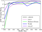
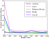
Effect of different buffer sizes We aim to investigate the effect of using different buffer sizes for visual tracking. Motivated by this, a quantitative evaluation of the proposed tracking algorithm is performed in nine different cases of buffer size. Meanwhile, we compute the average CLE and VOR for each video sequence in each case of buffer size. Fig. 1 shows the quantitative CLE and VOR performance on five video sequences. It is clear that the average CLE (VOR) decreases (increases) as the buffer size increases, and plateaus with approximately more than 300 samples.

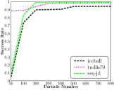
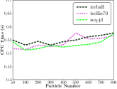
Evaluation of different particle numbers In general, more particle numbers enable visual trackers to locate the object more accurately, but lead to a higher computational cost. Thus, it is crucial for visual trackers to keep a good balance between accuracy and efficiency using a moderate number of particles. Motivated by this, we examine the tracking performance of the proposed tracking algorithm with respect to different particle numbers. The left part of Fig. 2 shows the average VOC success rates (i.e., $\frac{\#\mbox{success frames}}{\#\mbox{total frames}}$) of the proposed tracking algorithm on three video sequences. From the left part of Fig. 2, we can see that the success rate rapidly grows with the increase of particle number and finally converges. The right part of Fig. 2 displays the average CPU time (spent by the proposed tracking algorithm in each frame) with different particle numbers. It is observed from the right part of Fig. 2 that the average CPU time slowly increase.

Figure 3: Quantitative evaluation of the proposed tracker with/without metric learning on two video sequences. The top two subfigures are associated with the tracking performance in CLE and VOR on the “cubicle” video sequence, respectively; the bottom two subfigures correspond to the tracking performance in CLE and VOR on the “football” video sequence, respectively.

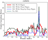
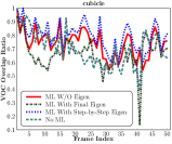
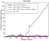
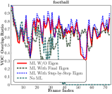
Performance with and without metric learning Metric learning is able to improve the intra-class compactness and inter-class separability of samples. In metric learning, three types of learning mechanisms can be used, including no eigendecomposition, step-by-step eigendecomposition, and final eigendecomposition [17]. To justify the effect of different metric learning mechanisms, we design several experiments on four video sequences. Fig. 3 shows the corresponding experimental results of different metric learning mechanisms in both CLE and VOR on two of the four video sequences (note that the results for the other two video sequences can be found in the supplementary file). Tab. 1 reports the average success rates of different metric learning mechanisms on the four video sequences. From Fig. 3 and Tab. 1, we can see that the performance of metric learning is better than that of no metric learning. In addition, the performance of metric learning with no eigendecomposition is close to that of metric learning with step-by-step eigendecomposition, and better than that of metric learning with final eigendecomposition. Therefore, the obtained results are consistent with those in [17]. Besides, metric learning with step-by-step eigendecomposition is much slower than that with no eigendecomposition which is adopted by the proposed tracking algorithm.

	cubicle	football	iceball	trellis70
ML w/o eigen	0.98	0.88	0.93	0.98
ML with final eigen	0.94	0.74	0.90	0.94
ML with step-by-step eigen	0.98	0.90	0.95	0.99
No metric learning	0.86	0.36	0.88	0.91

Table 1: Quantitative evaluation of the proposed tracker with/without metric learning on four video sequences The table reports their average success rates for each video sequence.

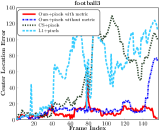
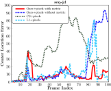
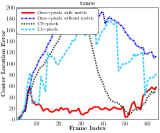
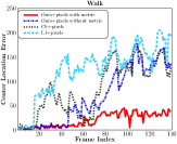
Comparison of different linear representations The objective of this task is to evaluate the performance of four types of linear representations including our linear representation with metric learning, our linear representation without metric learning, compressive sensing linear representation [4], and $\ell_{1}$-regularized linear representation [2]. For a fair comparison, we utilize the raw pixel features which are the same as [4, 2]. Fig. 4 shows the performance of these four linear representation methods in CLE on four video sequences. Clearly, our linear representation with metric learning consistently achieves lower CLE performance in most frames than the three other linear representations.

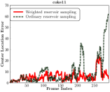
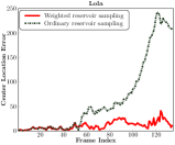
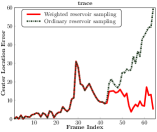
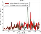
Evaluation of different sampling methods Reservoir sampling [18] addresses the problem of randomly drawing the uniformly distributed samples in a sequential manner. Following the work of [18], a weighted version of reservoir sampling is proposed in [21], which assign different weights to the samples occurring at different time points. Based on this weighed reservoir sampling method, the proposed tracking algorithm is capable of adaptively updating the sample buffer as tracking proceeds. Here, we aim to examine the performance of the two sampling methods. Fig. 5 shows the experimental results of the two sampling methods in CLE on four video sequences (note that the VOR results for these four video sequences can be found in the supplementary file). From Fig. 5, we can see that weighted reservoir sampling performs better than ordinary reservoir sampling.

Figure 4: Quantitative comparison of different linear representation methods in CLE on four video sequences (i.e., “football3”, “seq-jd”, “trace”, and “Walk”).

Figure 5: Quantitative comparison of different sampling methods in CLE on four video sequences (i.e., “coke11”, “Lola”, “trace”, and “Walk”). Before exceeding the buffer size limit (approximately occurring between frame 40 and frame 50), the performances of different sampling methods are identical.

Figure 6: Quantitative comparison of different trackers in CLE on the first eight video sequences.

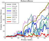
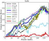
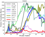
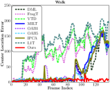
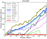
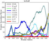
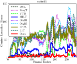
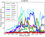
Comparison of competing trackers Fig. 6 plots the frame-by-frame center location errors (highlighted in different colors) obtained by the nine trackers for the first eight video sequences. Tab. 2 reports the success rates of the nine trackers over the thirteen video sequences. From Fig. 6 and Tab. 2, we observe that the proposed tracking algorithm achieves the best tracking performance on most video sequences.

Discussion Overall, the proposed tracking algorithm has the following properties. First, after the buffer size exceeds a certain value (around $300$ in our experiments), the tracking performance keeps stable with an increasing buffer size, as shown in Fig. 1. This is desirable since we do not need a large buffer size to achieve promising performance. Second, in contrast to many existing particle filtering-based trackers whose running time is typically linear in the number of particles, our method’s running time is sublinear in the number of particles, as shown in Fig. 2. Moreover, its tracking performance rapidly improves and finally converge to a certain value, as shown in Fig. 2. Third, as shown in Fig. 3 and Tab. 1, the performance of our metric learning with no eigendecomposition is close to that of computationally expensive metric learning with step-by-step eigendecomposition. Fourth, based on linear representation with metric learning, it performs better in tracking accuracy, as shown in Fig. 4. Fifth, it utilizes weighed reservoir sampling to effectively maintain and update the foreground and background sample buffers for metric learning, as shown in Fig. 5. Last, compared with other state-of-the-art trackers, it is capable of effectively adapting to complicated appearance changes in the tracking process by constructing an effective metric-weighted linear representation with weighed reservoir sampling, as shown in Fig. 6 and Tab. 2.

4 Conclusion

We have proposed a robust visual tracker based on non-sparse linear representations, which can be solved extremely efficiently in closed-form. Compared with recent sparse linear representation based trackers [2, 4], even with this simple implementation, our tracker is already much faster with comparable accuracy. To further improve the discriminative capacity of the linear representation, we have presented online Mahalanobis distance metric learning, which is able to capture the correlation information between feature dimensions. We empirically show that combining a metric into the linear representation considerably improve the robustness of the tracker. To make the online metric learning even more efficient, for the first time, we design a learning mechanism based on time-weighted reservoir sampling. With this mechanism, recently streamed samples in the video are assigned more importance weights. We have also theoretically proved that metric learning based on the proposed reservoir sampling with limited-sized sampling buffers can effectively approximate metric learning using all the received training samples. Compared with a few state-of-the-art trackers on thirteen challenging sequences, we empirically show that our method is more robust to complicated appearance changes, pose variations, and occlusions, etc.

Acknowledgments This work is in part supported by ARC Discovery Project (DP1094764).

	Ours	DML	FragT	VTD	MILT	OAB1	OAB5	IPCA	L1T
B-Beam	0.94	0.43	0.25	0.56	0.37	0.37	0.43	0.34	0.43
Lola	0.80	0.18	0.11	0.07	0.03	0.01	0.08	0.06	0.07
trace	0.89	0.12	0.63	0.11	0.42	0.40	0.42	0.31	0.06
Walk	0.98	0.67	0.09	0.11	0.64	0.62	0.67	0.62	0.11
football	0.88	0.20	0.47	0.62	0.07	0.05	0.05	0.01	0.07
iceball	0.93	0.59	0.52	0.70	0.16	0.14	0.12	0.09	0.08
coke11	0.87	0.37	0.05	0.10	0.28	0.04	0.04	0.03	0.04
trellis70	0.98	0.90	0.40	0.37	0.34	0.13	0.03	0.38	0.34
dograce	0.97	0.60	0.49	0.47	0.67	0.67	0.23	0.87	0.87
football3	0.97	0.46	0.32	0.31	0.61	0.87	0.24	0.22	0.16
car11	0.99	0.92	0.08	0.43	0.08	0.39	0.33	0.99	0.59
cubicle	0.98	0.82	0.37	0.20	0.22	0.22	0.21	0.25	0.49
seq-jd	0.95	0.85	0.88	0.79	0.61	0.58	0.38	0.45	0.61

Table 2: The quantitative comparison results of the nine trackers over the thirteen video sequences. The table reports their tracking success rates over each video sequence.

References

- [1] D. A. Ross, J. Lim, R. Lin, and M. Yang, “Incremental learning for robust visual tracking,” Int. J. Comp. Vis., vol. 77, no. 1, pp. 125–141, 2008.
- [2] X. Mei and H. Ling, “Robust visual tracking and vehicle classification via sparse representation,” IEEE Trans. Pattern Anal. Mach. Intell., 2011.
- [3] J. Kwon and K. M. Lee, “Visual tracking decomposition,” in Proc. IEEE Conf. Comp. Vis. Patt. Recogn., 2010, pp. 1269–1276.
- [4] H. Li, C. Shen, and Q. Shi, “Real-time visual tracking with compressive sensing,” in Proc. IEEE Conf. Comp. Vis. Patt. Recogn., 2011.
- [5] S. Hare, A. Saffari, and P.H.S. Torr, “Struck: Structured output tracking with kernels,” in Proc. IEEE Int. Conf. Comp. Vis., 2011.
- [6] X. Li, W. Hu, Z. Zhang, X. Zhang, and G. Luo, “Robust visual tracking based on incremental tensor subspace learning,” in Proc. IEEE Int. Conf. Comp. Vis., 2007, pp. 1–8.
- [7] X. Li, A. Dick, H. Wang, C. Shen, and A. van den Hengel, “Graph mode-based contextual kernels for robust SVM tracking,” in Proc. IEEE Int. Conf. Comp. Vis., 2011, pp. 1156–1163.
- [8] X. Li, W. Hu, H. Wang, and Z. Zhang, “Robust object tracking using a spatial pyramid heat kernel structural information representation,” Neurocomputing, vol. 73, no. 16-18, pp. 3179–3190, 2010.
- [9] C. Shen, J. Kim, and H. Wang, “Generalized kernel-based visual tracking,” IEEE Trans. Circuits & Systems for Video Tech., vol. 20, no. 1, pp. 119–130, 2010.
- [10] Q. Shi, A. Eriksson, A. van den Hengel, and C. Shen, “Is face recognition really a compressive sensing problem?,” in Proc. IEEE Conf. Comp. Vis. Patt. Recogn., 2011.
- [11] R. Rigamonti, M. A. Brown, and V. Lepetit, “Are sparse representations really relevant for image classification?,” in Proc. IEEE Conf. Comp. Vis. Patt. Recogn., 2011, pp. 1545–1552.
- [12] L. Zhang, M. Yang, and X. Feng, “Sparse representation or collaborative representation: Which helps face recognition?,” in Proc. IEEE Int. Conf. Comp. Vis., 2011.
- [13] K.Q. Weinberger, J. Blitzer, and L.K. Saul, “Distance metric learning for large margin nearest neighbor classification,” in Proc. Adv. Neural Inf. Process. Syst., 2006.
- [14] C. Shen, J. Kim, L. Wang, and A. van den Hengel, “Positive semidefinite metric learning with boosting,” in Proc. Adv. Neural Inf. Process. Syst., 2009, pp. 1651–1659.
- [15] X. Wang, G. Hua, and T. Han, “Discriminative tracking by metric learning,” Proc. Eur. Conf. Comp. Vis., pp. 200–214, 2010.
- [16] N. Jiang, W. Liu, and Y. Wu, “Adaptive and discriminative metric differential tracking,” in Proc. IEEE Conf. Comp. Vis. Patt. Recogn., 2011, pp. 1161–1168.
- [17] G. Chechik, V. Sharma, U. Shalit, and S. Bengio, “Large scale online learning of image similarity through ranking,” J. Mach. Learn. Research, vol. 11, pp. 1109–1135, 2010.
- [18] J. S. Vitter, “Random sampling with a reservoir,” ACM Trans. Math. Software, vol. 11, no. 1, pp. 37–57, 1985.
- [19] P. Zhao, S.C.H. Hoi, R. Jin, and T. Yang, “Online AUC maximization,” in Proc. Int. Conf. Mach. Learn., 2011.
- [20] M. Kolonko and D. Wäsch, “Sequential reservoir sampling with a non-uniform distribution,” ACM Trans. Math. Software, vol. 32, pp. 257–273, 2004.
- [21] P. S. Efraimidis and P. G. Spirakis, “Weighted random sampling with a reservoir,” Information process. letters, vol. 97, no. 5, pp. 181–185, 2006.
- [22] A. Jennings and J. McKeown, Matrix computation, John Wiley & Sons Inc., 1992.
- [23] A. S. Householder, The theory of matrices in numerical analysis, Blaisdell Publishing Co.: New York, 1964.
- [24] M. J. D. Powell, “A theorem on rank one modifications to a matrix and its inverse,” The Computer Journal, vol. 12, no. 3, pp. 288–290, 1969.
- [25] K. Crammer, O. Dekel, J. Keshet, S. Shalev-Shwartz, and Y. Singer, “Online passive-aggressive algorithms,” J. Mach. Learn. Research, vol. 7, pp. 551–585, 2006.
- [26] N. Dalal and B. Triggs, “Histograms of oriented gradients for human detection,” in Proc. IEEE Conf. Comp. Vis. Patt. Recogn., 2005.
- [27] X. Li, W. Hu, Z. Zhang, X. Zhang, M. Zhu, and J. Cheng, “Visual tracking via incremental log-euclidean riemannian subspace learning,” in Proc. IEEE Conf. Comp. Vis. Patt. Recogn., 2008, pp. 1–8.
- [28] A. Adam, E. Rivlin, and I. Shimshoni, “Robust fragments-based tracking using the integral histogram,” in Proc. IEEE Conf. Comp. Vis. Patt. Recogn., 2006, pp. 798–805.
- [29] B. Babenko, M. Yang, and S. Belongie, “Visual tracking with online multiple instance learning,” in Proc. IEEE Conf. Comp. Vis. Patt. Recogn., 2009, pp. 983–990.
- [30] H. Grabner, M. Grabner, and H. Bischof, “Real-time tracking via on-line boosting,” in Proc. British Machine Vis. Conf., 2006, pp. 47–56.