SPIN GLASS
A BRIDGE BETWEEN QUANTUM COMPUTATION AND STATISTICAL MECHANICS

Abstract

In this chapter, we show two fascinating topics lying between quantum information processing and statistical mechanics. First, we introduce an elaborated technique, the surface code, to prepare the particular quantum state with robustness against decoherence. Interestingly, the theoretical limitation of the surface code, accuracy threshold, to restore the quantum state has a close connection with the problem on the phase transition in a special model known as spin glasses, which is one of the most active researches in statistical mechanics. The phase transition in spin glasses is an intractable problem, since we must strive many-body system with complicated interactions with change of their signs depending on the distance between spins. Fortunately, recent progress in spin-glass theory enables us to predict the precise location of the critical point, at which the phase transition occurs. It means that statistical mechanics is available for revealing one of the most interesting parts in quantum information processing. We show how to import the special tool in statistical mechanics into the problem on the accuracy threshold in quantum computation.

Second, we show another interesting technique to employ quantum nature, quantum annealing. The purpose of quantum annealing is to search for the most favored solution of a multivariable function, namely optimization problem. The most typical instance is the traveling salesman problem to find the minimum tour while visiting all the cities. In quantum annealing, we introduce quantum fluctuation to drive a particular system with the artificial Hamiltonian, in which the ground state represents the optimal solution of the specific problem we desire to solve. Induction of the quantum fluctuation gives rise to the quantum tunneling effect, which allows nontrivial hopping from state to state. We then sketch a strategy to control the quantum fluctuation efficiently reaching the ground state. Such a generic framework is called quantum annealing. The most typical instance is quantum adiabatic computation based on the adiabatic theorem. The quantum adiabatic computation as discussed in the other chapter, unfortunately, has a crucial bottleneck for a part of the optimization problems. We here introduce several recent trials to overcome such a weakpoint by use of developments in statistical mechanics.

Through both of the topics, we would shed light on the birth of the interdisciplinary field between quantum mechanics and statistical mechanics.

1 Introduction: Statistical Mechanics and Quantum Mechanics

Quantum mechanics is a method partially based on the concept of the probability in outputs of the measurements on the physical state. This is because the physical state is allowed to be expressed by superposition of the possible eigenstates with the probability amplitude, which can be determined by the Schrödinger equation. Readers might feel uneasy since such a probabilistic phenomena seems to be problematic and uncontrollable. However, as shown in this chapter, several techniques have been designed and proposed for realization of the stability in quantum systems.

The quantum state is fragile, sensitive to noisy environment effects and continues to change. This peculiar destruction of the quantum state is known as decoherence. If we control to maintain the original state, we have to cure the quantum state suffering from undesired errors due to decoherence. The technique to remove these errors is the quantum error correction, which occupies the first part of this chapter. To fix successfully the quantum state, we need to prepare the redundant degrees of freedom to restore the original property and check where and how errors exist. We must thus design and deal with a many-body quantum system, which is known as an intractable problem. However it is worthwhile to strive such a difficult problem. Once you obtain an ingenious way to keep the quantum state, you find a pavement toward the realization of the quantum information processing, since you can encode simultaneously multiple information in the single quantum state by use of superposition. We here introduce a quantum error correcting technique, surface code [1], which skillfully use the concept of the topology to encode the original state in quantum many-body system. The surface code has a remarkable feature closely related with the main concept of this chapter. The accuracy threshold, which represents the theoretical limitation to restore the original quantum state by the surface code, is related with the phase transition in the special model in spin glasses [2]. Spin glass is a disordered magnetic material, which shows a peculiar behavior with extraordinary slow relaxation toward equilibrium state in a low temperature [3, 4, 5, 6, 7]. The complicated interactions in spin glasses spoil several methods used for systematic analyses in statistical mechanics. The identification of the critical point in spin glasses is used to be an intractable problem for long days. Fortunately, the recent development of theory in spin glasses yields a systematic analysis for its precise location. It means that the specialized tool to analyses in spin glasses is available for the problem in quantum computation. We show the fascinating connection between two unrelated topics, while reviewing the systematic approach to derive the accuracy threshold.

By using such a technique to maintain the quantum state as introduced above, we can prepare a coherent state. Then, how do we use superposition of the quantum system? Superposition enables us to evolve the quantum system in a parallel way over the various possible states. A famous algorithm given by Shor [8] is also based on the simultaneous search over all the possible candidates. In the second part of the present chapter, we introduce a generic technique by use of quantum nature in this chapter, called quantum annealing [9, 10, 11, 12, 13, 14, 15, 16]. Quantum annealing is an active use of superposition in order to obtain the most important result by searching all the candidates. Its attractive feature is simplicity and generality in applications. This is useful to solve several particular issues known as the optimization problems, in which we desire to find a minimizer or maximizer of the given multivariable function [17, 18]. The Shor’s algorithm uses a skillful technique in order to efficiently provide a desired answer. On the other hand, quantum annealing basically takes a simpler way only by controlling quantum fluctuations. The most typical procedure of quantum annealing, quantum adiabatic computation, is superior to its classical counterpart, simulated annealing [19, 20], owing to usage of quantum fluctuation. However a bottleneck of quantum adiabatic computation is also revealed in the application to the particular optimization problems. This weak point can be understood thorough a special mapping from the classical stochastic time evolution to the particular quantum dynamics. We are again between statistical mechanics and quantum information processing. Therefore, in this chapter, we will go further to overcome the bottleneck of quantum adiabatic computation by use of this fascinating relationship. We show several attempts for surmounting the obstacle involved in quantum adiabatic computation by employing several alternative strategies from statistical mechanics.

Statistical mechanics uses the probability similarly to quantum mechanics, but is capable to predict a definite behavior in the future in a large-number of components called as thermodynamic limit. The mathematical background of statistical mechanics, large deviation, provides the ability to give a definite answer even by use of the probability. Observant readers can find out the key point in this chapter. That is to deal with a large number of components. Turning on our eyes on substances around our daily life, they shows stable appearance. Material consists of many components, atoms, molecules and their mixtures, which should follow the rules of the quantum mechanics. The stability of these macroscopic systems comes from the particular property of the collection of many components. However, in many body systems, once if you tune the external parameters as temperature, pressure, and some fields, they can eventually change their uniform appearances. For instance, increase of temperature makes change of solid into liquid and gas. This phenomena is known as the phase transition. The phase transition involves singularities in the behavior of the physical quantities. The both of quantum error correction and quantum annealing shown in this chapter, suffer from this peculiar behavior. The failure to keep the quantum state by the surface code and the decay of the performance in quantum adiabatic computation come from the properties of the phase transition. Therefore, by dealing with the problems on the phase transition, we study the fascinating interdisciplinary connection between statical mechanics and quantum information processing.

Recent developments in manufacturing and manipulation of the quantum mechanical system enables us to prepare a large number of components. In this sense, the topics we deal with in this chapter must be valuable for developments in actual applications in the future.

2 Training: Statistical Mechanics

For unfamiliar readers with statistical mechanics and many students to understand the essential parts in this chapter, let us get back to the starting point of statistical mechanics.

At first let us recall the concept of the probability. What was the probability? If you have a non-tricky coin, you can say that the probability you can find a face (head or tail) should be a half. What does it mean?

2.1 Student’s misreading point: probability is…

We use an artificial variable with a binary $S=\pm 1$ to represent the coin state as head ($+1$) or tail ($-1$). A non-tricky coin takes the probability as $P_{1}(S=1)=1/2$ and $P_{1}(S=-1)=1/2$. We also can deal with a tricky coin with a biased probability as

$$P_{1}(S)=\frac{\exp(KS)}{Z_{1}(\beta)},$$ (1)

where $K$ is the strength of bias, and $Z_{1}(K)$ is a normalized constant explicitly given as $2\cosh K$. By use of the above probability, we can evaluate two characteristic quantities of the probabilistic system. The first quantity is expectation expressed as $m$, which indicates tendency of the coin whether head or tail,

$$m=\sum_{S=\pm 1}SP_{1}(S)=\tanh(K).$$ (2)

It readily shows that the coin state tends to be head if we increase the bias of the tricky coin $K\to\infty$. Another is the variance defined through the square of the difference from the expectation as

$$\sigma^{2}=\sum_{S}(S-m)^{2}P_{1}(S)=1-\tanh^{2}(K).$$ (3)

If we increase the bias $K$, the variance can vanish. However this is the case you know that this coin must be head without any probabilistic factors because $P_{1}(S=-1)\to 0$.

Then, if you once glance at the result of the single trial, can you judge whether its behavior is closely related with the obtained value of $m$ or not? The answer is ”No”. The value of $m$ only gives ”tendency”. The actual results will fluctuate around the expectation in repeating observations. We must repeat the coin games many times.

The above is the usual statement around the explanation of the probability. Since students, who studied the probability theory or other related topics, do not find out its genuine meaning, they often say that “probability” is obscure, abstract, and difficult!!, and conclude that it is not a well-understandable concept. Unfortunately, quantum mechanics and statistical mechanics with the concept of probability might be considered as non-reliable and non-deterministic to predict the future-coming behavior of the system we deal with. I would like to ask you why the probability for a non-tricky coin was a half. The students must recognize what the expectation express in our future. As you know, the expectation is not relevant for understanding the output in a single coin game. Let us play the game repeatedly. Then…

2.2 Probability describes… a certain behavior

In order to clarify the concept of the probability, in particular expectation, let us consider to accumulate the results of $N$-time observations after flipping coins. In all the trials, their results are characterized by the individually and independent distribution, which is same as in Eq. (1). Gradually approaching the specific example of use of probability in statistical mechanics, we take a simple model of the magnetic material, which is the typical example of studies in this field.

Let us introduce the Ising variable, which describes the magnetic momentum of spins in the magnetic material, often simply termed as “spin” or “Ising spin”. The Ising spin takes only two integers as $\pm 1$. We here regard the behavior of $N$-independent spins as the flipping coins in the $N$-sequential times. In statistical mechanics, we choose the specific probability distribution depending on the conditions of the system under consideration in order to calculate the expectation. Notice that, in statistical mechanics, the probability distribution can be given ”a priori” similarly to the above case of a non-tricky coin. In the previous simple case, we could choose a half as the probability for the coin since it was reasonable. Generally we do not know the precise structure of the probability distribution for various events. On the other hand, statistical mechanics provides us with the probability distribution of the behavior in equilibrium state. For instance, for the equilibrium state without change of the number of components, we use the canonical distribution characterized by the Hamiltonian and temperature.

$$P(S_{1},S_{2},\cdots,S_{N})=\frac{1}{Z_{N}(\beta)}\exp\left(-\beta H(S_{1},S_{2},\cdots,S_{N})\right),$$ (4)

where we define the inverse temperature $\beta=1/k_{B}T$ (often $k_{B}=1$) and $Z_{N}(\beta)$ is called as the partition function. The Hamiltonian describes the energy depending on the microscopic state of the system. The temperature controls thermal fluctuation to drive microscopic degrees of freedom in the system. If $\beta\to 0$, the spins are not stable due to strong effect by thermal fluctuation. On the other hand, in the low temperature $\beta\to\infty$, the system is settled into a lower energy state. The single spin favors parallel direction to the magnetic field since its energy can be described by the Hamiltonian $H(S)=-hS$, where $h$ is the strength of the magnetic field. Then the joint probability of the $N$ spins ($N$-time coin games) can be written by the canonical distribution as

$$P_{N}(S_{1},S_{2},\cdots,S_{N})=\frac{1}{Z_{N}(\beta)}\prod_{i=1}^{N}\exp(\beta hS_{i}),$$ (5)

where

$$Z_{N}(\beta)=\left(2\cosh(\beta h)\right)^{N}.$$ (6)

The partition function plays a roll of the characteristic function. Its logarithmic function is called the free energy $-\beta F_{N}(\beta)=\log Z_{N}(\beta)$. We often use the thermal average by use of the canonical distribution in statistical mechanics written as

$$\langle O\rangle=\sum_{\{S_{i}\}}O(\{S_{i}\})P_{N}(S_{,}S_{2},\cdots,S_{N}).$$ (7)

where $O$ denotes the physical observable.

Let me ask the following question. If you have huge number of the outputs in an experiment, how do you interpret the result. Usually we use the average over all the realizations to simplify the outputs. This simplified picture is often called as coarse graining in statistical mechanics. What we must take care of is that the average (sample mean) over all the realizations

$$m_{N}=\frac{1}{N}\sum_{i=1}^{N}S_{i},$$ (8)

and its variance

$$\sigma_{N}=\frac{1}{N}\sum_{i=1}^{N}(S_{i}-m_{N})^{2}.$$ (9)

Statistical mechanics gives a definite future of the above average for the many-body system in terms of the expectation and variance estimated from the specific distribution function.

Below let us see the connection between quantities given by the empirical measure and those by the a priori distribution function.

2.3 Large deviation property

We do not care the detail on the system with the large-number components. For instance, for the above $N$ spin systems, it is enough to characterize the magnetic property by the average of the $N$ Ising spins. This is called as the magnetization, which indicates the magnetic strength of the material. Statistical mechanics predicts such significant quantities in the macroscopic scale by averages over all the components, coarse-grained quantities. If we consider the large-number limit $N\to\infty$, the averaged values can correspond to the expectations estimated by the probability distribution under a certain condition shown below. It is convenient to change the expression of the joint probability (5) into the form of the probability of the average as

$$P_{N}(m)=\sum_{\{S_{i}\}}\delta\left(m-\frac{1}{N}\sum_{i=1}^{N}S_{i}\right)P_{N}(S_{1},S_{2},\cdots,S_{N}).$$ (10)

By use of the integral form of the delta function as

$$\delta\left(x\right)=\int^{\mathrm{i}\infty}_{-\mathrm{i}\infty}d\tilde{x}\exp(x\tilde{x}),$$ (11)

we can obtain

$$P_{N}(m)\propto\sum_{\{S_{i}\}}\int d\tilde{m}\exp\left\{Nm\tilde{m}+\left(-\tilde{m}\sum_{i=1}^{N}S_{i}+\beta h\sum^{N}_{i=1}S_{i}\right)\right\}.$$ (12)

Before performing the integration, we sum over the spin variables.

$$P_{N}(m)\propto\int d\tilde{m}\exp\left\{Nm\tilde{m}+N\log\left(2\cosh\left(\beta h-\tilde{m}\right)\right)\right\}.$$ (13)

The integrand is proportional to $N$. In that case, we can apply the saddle-point method to the above integration. When we consider the infinite limit of $N$, the integral is given by the maximizer $\tilde{m}^{*}$ of the integrand as

$$P_{N}(m)=\exp\left\{-Nf(m,\tilde{m}^{*})\right\}.$$ (14)

Here we define the pseudo free energy $f(m,\tilde{m})$ as

$$f(m,\tilde{m})=-m\tilde{m}-\log\left(2\cosh\left(\beta h-\tilde{m}\right)\right).$$ (15)

The saddle-point equation for $\tilde{m}$, which gives the maximum of the integrand (or the minimum of the pseudo free energy), is

$$\frac{\partial f}{\partial\tilde{m}}=0\to m=\tanh\left(\beta h-\tilde{m}\right).$$ (16)

The maximizer of the integrand is given by $\tilde{m}^{*}=\beta h-\tanh^{-1}(m)$. By use of this maximizer, we obtain the probability of the magnetization as

$$P_{N}(m)=\exp\left\{N\left(m\beta h-m\tanh^{-1}m+\log\frac{2}{\sqrt{1-m^{2}}}\right)\right\}.$$ (17)

In Fig. 1, we describe the behavior of $f(m,\tilde{m}^{*})$.

Figure 1: Behavior of $f(m,\tilde{m}^{*})$ with $\beta h=1.0$ (solid), $0$ (thick symmetric dashed curve), and $-1.0$ (dotted curve).

The maximum is located at $m^{*}=\tanh(\beta h)$, which can be verified by derivative with respect to $m$. If $N$ increase, the probability away from $m^{*}=\tanh(\beta h)$ decrease exponentially. The maximum indicates the value of the expectation since

$$\langle m\rangle=\left\langle\frac{1}{N}\sum_{i=1}^{N}S_{i}\right\rangle=\frac{1}{N}\frac{\partial P_{N}(m)}{\partial\hat{m}}=\tanh(\beta h).$$ (18)

Moreover, if we evaluate the variance, we reach

$$\langle\sigma^{2}_{N}\rangle=\left\langle\frac{1}{N}\sum_{i=1}^{N}(S_{i}\right\rangle=\frac{1}{N}\frac{\partial^{2}P_{N}(m)}{\partial\hat{m}^{2}}=\frac{1}{N}\left(1-\tanh^{2}(\beta h)\right).$$ (19)

Therefore the magnetization can take a “definite” value $m^{*}=\tanh(\beta h)$ if $N\to\infty$. This property is known as the large deviation principle in mathematics. In the above simple case, we treat the individually-independent distribution. Fortunately, it is confirmed that the large deviation principle holds in relatively wide varieties rather than individually-independent distribution. Statistical mechanics plentifully uses explicitly and implicitly this fruitful property. It means that, in many-body system, we can predict a definite future even by use of the probability as classical mechanics with the deterministic equation. In other words, statistical mechanics predicts the average value for the physical observables of the system with large number components from the calculation of the expectation by use of an a priori distribution function such that the canonical, micro canonical, and ground canonical ensemble.

2.4 Mean-field analysis

The probability can give a definite future expressed by the expectation value, if we are interested in many-body systems by the support of the large deviation principle. However many degrees of freedom in material strongly interact with each other. The spin is not an exception. Differently from the above simplified case, we must take care of the effect through magnetic-dipole interactions to more precisely understand the behavior of magnetic material. We exemplify its simplest model to deal with effects of interactions known as the Ising model, whose Hamiltonian is

$$H=-J\sum_{\langle ij\rangle}S_{i}S_{j}.$$ (20)

The subscript stands for the index of the site, where the spin is located. The summation is taken over the nearest-neighboring pairs of spins. The geometric property as the locations of the spins is closely related with the structure of the magnetic material. As precisely as possible we analyze an actual behavior of magnetic material, we must consider a finite-dimensional structure of atoms. However it is difficult to straightforwardly perform nontrivial analyses on the finite-dimensional Ising model. We take several approximations or numerical simulations for obtaining meaningful results of the finite-dimensional Ising models. The exactly solvable examples without any approximations are found in one and two dimensions but rare exceptions.

The simple but qualitative approximation often taken as the first trial is the mean-field analysis. It enables us to obtain a meaningful picture to describe a peculiar behavior of the many-body system. The probability distribution of the degrees of freedom should be correlated with each other in the case of the existence of the interactions. However we simply assume that the probability distribution should be factorized as individually-independent one as in Eq. (5). As seen above, under this approximation, we can characterize the system by use of the magnetization $m$. In other words, the surrounding spins adjacent to a particular spin being replaced by a uniform variable $m$, we convert the many-body problem into a simple one-body system. Let us rewrite the Hamiltonian by the replacement of the surrounding spins $S_{j}=m$ to $S_{i}$ as

$$H_{\mathrm{MF}}(S_{i})=-\frac{zJm}{2}\sum_{i=1}^{N}S_{i},$$ (21)

where $z$ is the coordination number (usually in the case of the hyper cubic system, $z=2d$, where $d$ is the dimension). Similar calculations to the previous example give rise to the final expression of the probability for $m$ as

$$P_{N}(m)\propto\int d\tilde{m}\exp\left\{Nm\tilde{m}+N\log\left(2\cosh\left(\frac{\beta Jz}{2}m-\tilde{m}\right)\right)\right\}.$$ (22)

The saddle point equation is

$$\frac{\partial f}{\partial\tilde{m}}=0 \to m=\tanh\left(\beta\frac{Jzm}{2}-\tilde{m}\right).$$ (23)

Thus we find the probability of the magnetization for the interacting system

$$P_{N}(m)\propto\exp\left\{N\left(\frac{\beta Jz}{2}m^{2}-m\tanh^{-1}m-\log\frac{2}{\sqrt{1-m^{2}}}\right)\right\}.$$ (24)

We describe the behavior of the free energy as in Fig. 2

Figure 2: Behavior of $f(m,\tilde{m}^{*})$ for $z=6$, while we set $J=1$, with $\beta=0.0$ (solid), $0.1$ (dashed curve), and $0.25$ (dotted curve).

Readers can find two maximizers in the low-temperature region. Let us evaluate explicitly this unexpected result. The most probable state is given by the maximizer of the following self-consistent equation

$$m=\tanh(\beta Jzm).$$ (25)

The explicit value of the magnetization over all temperature is shown in Fig. 3.

Figure 3: Magnetization given by the mean-field analysis for the Ising model $z=6$. Here we set $J=1$.

Beyond the special point $\beta=1/zJ$, the magnetization suddenly take non-zero value despite of absence of magnetic field. This is the spontaneous symmetry breaking, in other terms, the phase transition. This is also a peculiar property in many-body systems. The mean-field analysis gives several meaningful properties including the phase transition on many-body systems as above. The results by the mean-field analysis can be validated in infinite dimensions and reflect on the behavior in such higher dimensions. Therefore we must take care of their applicability to the actual behavior of the many-body system in finite dimensions.

2.5 Phase transition

Let us more qualitatively discuss the phase transition through the results obtained by mean-field analysis. Without the magnetic field, the spins do not have any tendency of the direction, that is $m\approx 0$. Indeed the most probable state is given by $m=0$. This solution describes the paramagnetic phase of the magnetic material without any magnetization. However if you expand the self-consistent equation under the assumption that $m$ should be small as

$$m=\beta Jzm.$$ (26)

We find the special temperature $\beta=1/zJ$, at which the magnetization $m$ can take a non-zero value. This is a signature of the phase transition from the paramagnetic state into the ferromagnetic state. We expand the self-consistent equation up to third order of $m$, and thus obtain

$$m=\beta Jz\left\{m-\frac{1}{3}\left(\beta Jz\right)^{2}m^{3}\right\}.$$ (27)

This equation indeed gives the ferromagnetic solutions with non-zero magnetization as $m=\pm\sqrt{3(1-\beta Jz)}/(\beta Jz)$, which vanish at $\beta=1/zJ$. This special temperature is called the critical point. In addition, two phases, paramagnetic and ferromagnetic phases are characterized by the behavior of the magnetization. Such a quantity, which can distinguish the phase, is called as the order parameter. Could you find the fact that you have two ferromagnetic solutions of the magnetization? It implies that the two maximizers, say two probable states, are allowed to appear in Eq. (24). Then, which solution should be chosen and will appear naturally in experience? It depends on the dynamics rule and the initial conditions. If you design the dynamics to simulate thermal fluctuations At least, we can find the fact that, in the ferromagnetic phase, state with $m=0$ would not be expected to occur in the case with a large $N$. That means that two of the probable states are separate and can not change one into another in the actual experience. In other words, the system has some robustness against thermal fluctuations. That will be an analogous property to protect the fragile quantum state later.

2.6 Spin Glasses

The above exemplified model have a uniform interactions between the Ising spins. The theoretical model of spin glasses is usually not the case. The simplest model, the Edwards-Anderson model, is defined by the following Hamiltonian

$$H=-\sum_{\langle ij\rangle}J_{ij}S_{i}S_{j},$$ (28)

where $J_{ij}$ is the disordered interactions assumed to obey several type of the distribution functions. We often deal with two typical cases, which take a bimodal distribution (then called as $\pm J$ Ising model)

$$P(J_{ij})=p\delta(J_{ij}-J)+(1-p)\delta(J+J_{ij}),$$ (29)

and the Gaussian distribution with the average $J_{0}$ and the variance $J$

$$P(J_{ij})=\frac{1}{\sqrt{2\pi J^{2}}}\exp\left(-\frac{1}{2J^{2}}(J_{ij}-J_{0})^{2}\right).$$ (30)

The partition function should be dependent of the specific configuration as

$$Z(\beta;\{J_{ij}\})=\sum_{\{S_{i}\}}\prod_{\langle ij\rangle}\exp\left(\beta J_{ij}S_{i}S_{j}\right).$$ (31)

In order to evaluate the partition function and thus the free energy, we strive the difficult task to deal with the non-uniform interactions. Instead, we usually take a wise strategy to evaluate the averaged free energy based on the self-averaging property as, in the large-limit $N$,

$$\frac{1}{N}F(\beta;\{J_{ij}\})\to\frac{1}{N}\left[F(\beta;\{J_{ij}\})\right],$$ (32)

where the square bracket denotes the average over all the combinations of $\{J_{ij}\}$ (configurational average) and the free energy is defined as

$$-\beta F(\beta;\{J_{ij}\})=\log Z(\beta;\{J_{ij}\}).$$ (33)

The self-averaging property is valid for other observables, which can be obtained from the free energy per site. For instance, the magnetization per site satisfies

$$m=\frac{1}{N}\sum_{i=1}^{N}S_{i}=\langle S_{i}\rangle\to\left[\langle S_{i}\rangle\right].$$ (34)

The average through the logarithmic term is still the intractable task. The replica method is then useful to perform the configurational average for the free energy. First, we evaluate the averaged power of the partition function to the natural number $n$ as $\left[Z^{n}(\beta;\{J_{ij}\})\right]$. Then we consider the analytical continuation of $n$ and take the limit based on the elementary identity as

$$\left[\log Z(\beta;\{J_{ij}\})\right]=\lim_{n\to 0}\frac{\left[Z^{n}(\beta;\{J_{ij}\})\right]-1}{n}.$$ (35)

You see the replica method everywhere in analyses on spin glasses.

We avoid the complicated details of analytical results in spin glasses in order to straightforwardly understand the most important parts in this chapter. However we write down a few things on spin glasses related with our topics. The peculiar feature in spin glasses is the extraordinary slow relaxation toward equilibrium state in the low temperature. This is because the existence of many minima of the free energy on spin glasses revealed by the mean-field analysis. This fact implies that there are a large number of the most probable states. The number diverges exponentially as increase of the number of spins $N$. Unfortunately, this fact has been confirmed by the mean-field analysis. We have still not given the answer whether the actual finite-dimensional spin glasses follow the same scenario as that given by the mean-field analysis or not. The main reason of lack of understanding of finite dimensional spin glasses is absence of systematic tools to approach the issue. One of the exceptional methods would be the gauge theory.

2.7 Gauge theory

We take the $\pm J$ Ising model as an instance of the spin glass to show the detailed analysis. For simplicity, we combine the strength interaction with the inverse temperature as $K=\beta J$. We write the Hamiltonian of the $\pm J$ Ising model as

$$H=-\sum_{\langle ij\rangle}J\tau_{ij}S_{i}S_{j}.$$ (36)

The sign of the interactions follow the distribution function

$$P(\tau_{ij})=p\delta(\tau_{ij}-1)+(1-p)\delta(\tau_{ij}+1).$$ (37)

The partition function can be also written as $Z(K;\{\tau_{ij}\})$.

We then define the local transformation by a binary variable $\sigma_{i}=\pm 1$, called as the gauge transformation, as [7, 22]

$$\tau_{ij} \rightarrow \sigma_{i}\sigma_{j}\tau_{ij}$$ (38)

$$S_{i} \rightarrow \sigma_{i}S_{i}.$$ (39)

Notice that this transformation does not change the value of the physical quantity given by the average over $\tau_{ij}$ and $S_{i}$ since it alters only the order of the summations. The Hamiltonian can not change its form after the gauge transformation since the right-hand side is evaluated as

$$-\sum_{\langle ij\rangle}J\tau_{ij}\sigma_{i}\sigma_{j}\sigma_{i}S_{i}\sigma_{j}S_{j}=H.$$ (40)

As this case, if the physical quantity is invariant under the gauge transformation (gauge invariant), we can evaluate its exact value even for finite-dimensional spin glasses. The key point of the analysis by the gauge transformation is on the form of the distribution function. Before performing the gauge transformation, the distribution function can take the following form as

$$P(\tau_{ij})=\frac{\mathrm{e}^{K_{p}\tau_{ij}}}{2\cosh K_{p}},$$ (41)

where $\exp(-2K_{p})=(1-p)/p$. The gauge transformation changes this form, in a different way from the Hamiltonian, as

$$P(\tau_{ij})=\frac{\mathrm{e}^{K_{p}\tau_{ij}\sigma_{i}\sigma_{j}}}{2\cosh K_{p}}.$$ (42)

Let us evaluate the internal energy by aid of the gauge transformation here. The thermal average of the observables $O$ is defined as, by use of the canonical distribution

$$\langle O\rangle_{K} = \sum_{\{S_{i}\}}\frac{1}{Z(K;\{\tau_{ij}\})}O\prod_{\langle ij\rangle}\exp\left(K\tau_{ij}S_{i}S_{j}\right).$$ (43)

Then the thermal average of the Hamiltonian can be written as

$$\langle H\rangle_{K} = \sum_{\{S_{i}\}}\frac{1}{Z(K;\{\tau_{ij}\})}H\prod_{\langle ij\rangle}\exp\left(K\tau_{ij}S_{i}S_{j}\right)$$ (44)

$$= -J\frac{d}{dK}\log Z(K;\{\tau_{ij}\}).$$ (45)

We can use the self-averaging property here since this is given by the derivative of the free energy, and thus take the configurational average as

$$\left[\langle H\rangle_{K}\right]_{K_{p}} = \sum_{\{\tau_{ij}\}}\prod_{\langle ij\rangle}\frac{\exp(K_{p}\tau_{ij})}{2\cosh K_{p}}\times\langle H\rangle_{K},$$ (46)

where $[\cdots]_{K_{p}}$ denotes the configurational average with $K_{p}$. Then we perform the gauge transformation, which does not change the value of the internal energy

$$\left[\langle H\rangle_{K}\right]_{K_{p}} = \sum_{\{\tau_{ij}\}}\prod_{\langle ij\rangle}\frac{\exp(K_{p}\tau_{ij}\sigma_{i}\sigma_{j})}{2\cosh K_{p}}\times\langle H\rangle_{K}.$$ (47)

Therefore we here take the summation over all the possible configurations of $\{\sigma_{i}\}$ and divide it by $2^{N}$ (the number of configurations) as

$$\left[\langle H\rangle_{K}\right]_{K_{p}} = \frac{1}{2^{N}}\sum_{\{\sigma_{i}\}}\sum_{\{\tau_{ij}\}}\prod_{\langle ij\rangle}\frac{\exp(K_{p}\tau_{ij}\sigma_{i}\sigma_{j})}{2\cosh K_{p}}\times\langle H\rangle_{K}.$$ (48)

We take the summation over $\{\sigma_{i}\}$ in advance of that over $\{\tau_{ij}\}$ and then find the partition function with $K_{p}$ instead of $K$.

$$\left[\langle H_{K}\rangle\right]_{K_{p}} = \frac{1}{2^{N}}\sum_{\{\tau_{ij}\}}\frac{Z(K_{p};\{\tau_{ij}\})}{(2\cosh K_{p})^{N_{B}}}\times\langle H\rangle_{K}.$$ (49)

Going back to Eq. (44), we can delete both of the partition functions on the denominator and numerator by setting $K_{p}=K$ as

$$\left[\langle H\rangle_{K}\right]_{K} = \frac{-J}{2^{N}(2\cosh K_{p})^{N_{B}}}\sum_{\{S_{i}\}}\sum_{\{\tau_{ij}\}}\frac{d}{dK}\exp\left(K\tau_{ij}S_{i}S_{j}\right)$$ (50)

$$= -N_{B}\tanh K.$$

Similarly, we can evaluate the rigorous upper bound on the specific heat as well as the restriction on the structure of the phase diagram. The condition $K_{p}=K$ defines the special subspace in which we can perform the exact analysis even for finite-dimensional spin glasses. This subspace is called as the Nishimori line [7, 22]. On this subspace, we can reveal several rigorous properties on the structure of the phase diagram even for spin glasses by relatively simple calculations. For instance, let us consider to evaluate the local magnetization $\langle S_{i}\rangle$ by the gauge transformation. The local magnetization identifies the existence of the ferromagnetic order and its definition is

$$\langle S_{i}\rangle_{K}=\sum_{\{S_{i}\}}S_{i}\prod_{\langle ij\rangle}\frac{\exp(K\tau_{ij}S_{i}S_{j})}{Z(K;\{\tau_{ij}\})}.$$ (51)

Let us consider to evaluate its configurational average

$$\left[\langle S_{i}\rangle_{K}\right]_{K_{p}}=\sum_{\{\tau_{ij}\}}\prod_{\langle ij\rangle}\frac{\exp(K_{p}\tau_{ij})}{2\cosh K_{p}}\times\langle S_{i}\rangle_{K}.$$ (52)

After the gauge transformation, we obtain

$$\left[\langle S_{i}\rangle_{K}\right]_{K_{p}}=\sum_{\{\tau_{ij}\}}\sigma_{i}\prod_{\langle ij\rangle}\frac{\exp(K_{p}\tau_{ij}\sigma_{i}\sigma_{j})}{2\cosh K_{p}}\times\langle S_{i}\rangle_{K}.$$ (53)

By summing over all the possible configurations of the gauge variables and dividing the resulting equality by $2^{N}$, we reach

$$\left[\langle S_{i}\rangle_{K}\right]_{K_{p}}=\sum_{\{\tau_{ij}\}}\frac{Z(K_{p};\tau_{ij})}{2^{N}\left(2\cosh K_{p}\right)^{N}}\times\langle\sigma_{i}\rangle_{K_{p}}\times\langle S_{i}\rangle_{K}.$$ (54)

On the other hand, let us evaluate the configurational average of the product of the correlation functions with different temperatures as

$$\left[\langle\sigma_{i}\rangle_{K_{p}}\langle S_{i}\rangle_{K}\right]_{K_{p}}=\sum_{\{\tau_{ij}\}}\prod_{\langle ij\rangle}\frac{\exp(K_{p}\tau_{ij})}{2\cosh K_{p}}\times\langle\sigma_{i}\rangle_{K_{p}}\langle S_{i}\rangle_{K}.$$ (55)

On this equality, the gauge transformation only changes the sign of the interactions as $\tau_{ij}\rightarrow\tau_{ij}\sigma_{i}^{\prime}\sigma_{j}^{\prime}$ in the exponential function. We find the following equality by summing over $\{\sigma_{i}^{\prime}\}$ and multiplying $1/2^{N}$

$$\left[\langle S_{i}\rangle_{K}\right]_{K_{p}}=\left[\langle\sigma_{i}\rangle_{K_{p}}\langle S_{i}\rangle_{K}\right]_{K_{p}}.$$ (56)

Let us discuss the structure of the phase diagram of the $\pm J$ Ising model by use of this equality. Setting $K=K_{p}$, we obtain

$$\left[\langle S_{i}\rangle_{K_{p}}\right]_{K_{p}}=\left[\langle S_{i}\rangle_{K_{p}}^{2}\right]_{K_{p}}.$$ (57)

The quantity on the right-hand side is the order parameter of the spin-glass phase, called as the spin-glass parameter. In the spin-glass phase, the directions of the spins orient are random in space. Thus $m$ should be zero and it implies

$$m=\frac{1}{N}\sum_{i}S_{i}=\langle S_{i}\rangle\rightarrow\left[\langle S_{i}\rangle_{K_{p}}\right]_{K_{p}}\rightarrow 0.$$ (58)

On the other hand, if the spins are frozen, their square should be non-zero. Thus

$$q=\left[\langle S_{i}\rangle_{K_{p}}^{2}\right]_{K_{p}}\neq 0.$$ (59)

Therefore, on the Nishimori line, we prove that the spin-glass phase does not exist since the important fact $q=m$ is given by Eq. (57). In addition, if we take the absolute value of the magnetization away from the Nishimori line, we find

$$|\left[\langle S_{i}\rangle_{K}\right]_{K_{p}}|\leq|\left[\langle S_{i}\rangle_{K}\right]_{K_{p}}|\times|\left[\langle S_{i}\rangle_{K_{p}}\right]_{K_{p}}|\leq|\left[\langle S_{i}\rangle_{K_{p}}\right]_{K_{p}}|.$$ (60)

This inequality states that the magnetization takes the largest value on the Nishimori line along the vertical line of $K_{p}$. It implies that a special critical point, multicritical point, is located at the most left-hand side of the phase diagram as in Fig. 4.

Figure 4: Nishimori line and the typical phase diagram of the $\pm J$ Ising model. The vertical axis is the temperature, since $K$ can be regarded as the inverse temperature. The horizontal axis expresses the density of the ferromagnetic interactions in terms of $K_{p}$. The ferromagnetic, paramagnetic, and spin-glass phases are denoted by “F”, “P” and “SG”, respectively. The solid curve represent the phase boundary. The dashed curve describes the Nishimori line. The multicritical point is located at the most left-hand side.

In the following sections, we will find several problems on spin glasses, which are lying between statistical mechanics and quantum information processing. Although it is not enough to understand the whole properties on spin glasses, let us first go to these fascinating parts. After showing the interesting connections, we will strive the specific problems related with the spin glasses we must solve then.

3 Quantum error correction: surface code

In the first part of this chapter, we describe a technique for the quantum error correction. In order to protect the vulnerable quantum state from decoherence, we consider a method for circumvention of the effects from decoherence. It is very important to perform the quantum information processing. We here show an elaborated technique by use of the property of the topology. Our approach, in short terms, is based on encoding a few “logical” qubits in a particular state, which is not disturbed directly by noise of the “physical” qubits. Here we call the quantum state describing superposition of the binary state $0$ and $1$ (in terms of informatics, bits) as qubits This strategy is analogous to the classical counterpart, in which we introduce some redundancy to restore the original state.

3.1 Error model

The quantum state of the single qubit is written as

$$|\Psi\rangle=\alpha|0\rangle+\beta|1\rangle.$$ (61)

Here the above coefficients follow $|\alpha|^{2}+|\beta|^{2}=1$. We can write all the changes on the binary Hilbert space by combination of the identity operator and the Pauli operators $X$, $Y$ and $Z$.

$$X=\left(\begin{array}[]{cc}0&1\\ 1&0\end{array}\right),\quad Y=\left(\begin{array}[]{cc}0&\mathrm{i}\\ -\mathrm{i}&0\end{array}\right),\quad Z=\left(\begin{array}[]{cc}1&0\\ 0&-1\end{array}\right).$$ (62)

By this mean, we express the error by the action of the Pauli operator. The action of $X$ represents a phase error, and that of $Z$ expresses a flip error. In addition, $Y$ is a multiple error as $Y=\mathrm{i}XZ$.

Assuming the error will occur in a stochastic manner, let us define a noise model where the qubit gets errors as

$$\rho\to p_{I}\rho+\left(p_{X}X\rho X+p_{Y}Y\rho Y+p_{Z}Z\rho Z\right).$$ (63)

Although we can deal with any cases of $p_{I},p_{X},p_{Y}$, and $p_{Z}$, Let us start from the simple case with uncorrelated between the flip and phase errors as $p_{I}=(1-p)^{2}$ and $p_{X}=p_{Z}=p$, while $p_{Y}=p^{2}$, where $0\leq p\leq 1$. In this case, we can independently treat two of the errors. We must construct an ingenious procedure to recover the damaged qubits, that is the quantum error correction. Once an error occurs on the single qubit system, we can not remove the error, since we do not know the original state. The single qubits is too weak to save the specific information once error occurs. Therefore we need to prepare many qubits against errors as the first strategy. The first stage of the quantum error correction is thus to construct the many-body quantum system to store several bits of the information. That is analogous with the concept of redundancy in the classical information.

3.2 Surface code

Let us construct an array of qubits on a torus by setting qubits on each edge $(ij)$ of the square lattice embedded on a torus (genus $1$). Here we make two ways to describe the square lattice, while being unchanged of the location of the qubits, as in Fig. 5.

Figure 5: Square lattice (say original) and its dual on a torus. The location of the qubit is the center of the edge $(ij)$ (or $(i^{*}j^{*})$) denoted by the black square.

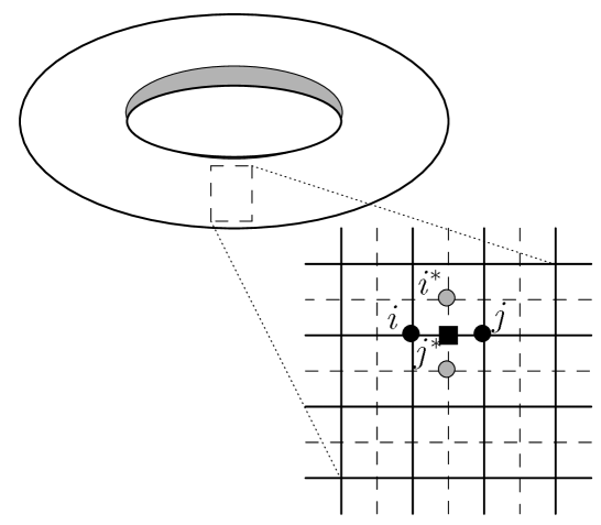
The original square lattice is convenient to explain how to detect and remove the flip errors and the other (dual) is for the phase errors. The embedded qubits (say physical qubits) on all the edges actually suffer from disturbance by noisy environment. We do not directly use the quantum state of these physical qubits to encode the information. Instead, we make the particular quantum state, which is stable against direct effects due to the errors. In order to construct such a fault-tolerant subspace, called as the codespace, for encoding the information, we define two of the check operators. One is the star operator for each site $s$ as

$$X_{s}=\otimes_{(ij)\in s}X_{(ij)},$$ (64)

and the other is the plaquette operator for each plaquette $p$

$$Z_{p}=\otimes_{(ij)\in p}Z_{(ij)},$$ (65)

where the product consists of four edges adjacent to each site and each plaquette as depicted in Fig. 6.

Figure 6: Star and plaquette operators.

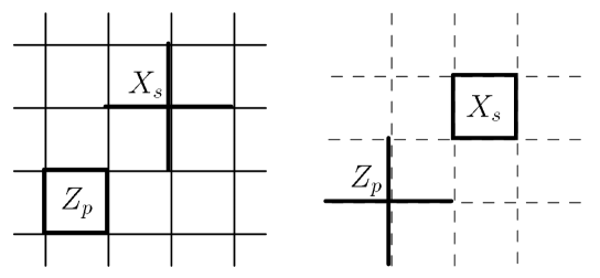
All of the star operators $X_{s}$ and the plaquette operators $Z_{p}$ commute and are thus simultaneously diagonalizable. The codespace to encode the specific information consists of their simultaneous $+1$ eigenstates of all the check operators as $X_{s}|\Psi_{c}\rangle=+1|\Psi_{c}\rangle$ for any $s$ and $Z_{p}|\Psi_{c}\rangle=+1|\Psi_{c}\rangle$ for any $p$. The site on the original square lattice is replaced by the plaquette on the dual one, and vice versa. The star operators are thus found to consist of the unit loops on the “dual” square lattices. Let us consider contractible loops on the surface of the torus denoted by $C$ and $C^{*}$ on the original and dual lattices, respectively. The action $C^{*}$ can be expressed by the product of $X_{s}$ as in Fig. 7.

Figure 7: Contractible loops $C$ and $C^{*}$ and their expressions by the check operators $X_{s}$ and $Z_{p}$.

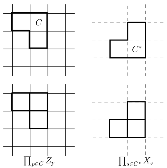
Here notice that the double action of the same Pauli operator becomes unity. On the other hand, the plaquette operators conform the unit loop on the original square lattice. Thus the action represented by any contractible loops on the original lattice $C$ is given by the product of $Z_{p}$ as in Fig. 7. The action described by $C$ and $C^{*}$ acts trivially on the codespace, since the codespace is the eigenspace of the star and plaquette operators. In other words, the compatible-loop actions by the Pauli operator $Z$ on the original lattice and $X$ on the dual one can not alter the particular quantum state encoded on the torus.

We here show the explicit form of the encoded quantum state below. Let us prepare a uniform linear-combination state of all the possible contractible loops with the products of $X_{s}$ and $Z_{p}$ as

$$|\Psi_{c}\rangle = \left(1+\sum_{s}X_{s}+\sum_{s_{1},s_{2}}X_{s_{1},s_{2}}+\cdots\right)$$ (66)

$$\quad\times\left(1+\sum_{p}Z_{p}+\sum_{p_{1},p_{2}}Z_{p_{1}}Z_{p_{2}}+\cdots\right)|\Psi_{0}\rangle,$$

where $|\Psi_{0}\rangle$ is the vacuum state of the physical qubits. Then we can easily confirm that $X_{s}|\Psi_{c}\rangle=|\Psi_{c}\rangle$ and $Z_{p}|\Psi_{c}\rangle=|\Psi_{c}\rangle$.

On the other hand, any non-contractible loop, winding around the torus, of the Pauli operators of $X$ and $Z$ can map the codespace to itself in a nontrivial manner, since the possible combinations of the contractible loops never constitute any non-contractible loops, while such an operator can commute with any star and plaquette operators. If we set $L\times L$ lattice on a torus, we have $2L^{2}$ physical qubits and $2(L^{2}-1)$ check operators. The remaining degrees of freedom of $2$ implies existence of two non-contractible loops, winding around the hole of the torus $L_{v}$ and winding around the body of the torus $L_{t}$ as depicted in Fig. 8.

Figure 8: Non-contractible loops $L_{v}$ and $L_{t}$ and the logical operators.

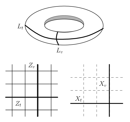
Let us express these non-contractible loops on the torus in terms of the products of Pauli operators as

$$\bar{X}_{v} = \prod_{(ij)\in L_{v}}X_{(ij)}$$ (67)

$$\bar{X}_{t} = \prod_{(ij)\in L_{t}}X_{(ij)}$$ (68)

$$\bar{Z}_{v} = \prod_{(ij)\in L^{*}_{v}}Z_{(ij)}$$ (69)

$$\bar{Z}_{t} = \prod_{(ij)\in L^{*}_{t}}Z_{(ij)}.$$ (70)

They are termed as logical operators. Here we use the asterisk denoting the non-contractible loop on the dual lattice. The combinations of non-contractible loops yield $2^{4}=16$ different homology classes embedded in the original and dual square lattices on the single torus. The elementary manipulation confirms that the logical operators can form Pauli algebra of two effective qubits encoded in the topological degrees of freedom on the torus as $[\bar{Z}_{v},\bar{Z}_{t}]=[\bar{X}_{v},\bar{X}_{t}]=0$, while $\bar{X}_{v}\bar{Z}_{t}=-\bar{Z}_{t}\bar{X}_{v}$ and $\bar{X}_{t}\bar{Z}_{v}=-\bar{Z}_{v}\bar{X}_{t}$. Thus, by use of these algebras by the non-contractible loops on the torus, we can prepare a $4\times 4$ Hilbert space, say two logical qubits, explicitly given by $|\Psi_{k_{1},k_{2},k_{3},k_{4}}\rangle=Z^{k_{1}}_{v}Z^{k_{2}}_{t}X^{k_{3}}_{v}X^{k_{4}}_{t}|\Psi_{c}\rangle$, where $k_{i}$ is the number taking $0$ and $1$ to distinguish the basis of the logical qubits. The logical qubits is in general written as

$$|\Psi\rangle=\sum_{k_{1},k_{2},k_{3},k_{4}}A_{k_{1},k_{2},k_{3},k_{4}}|\Psi_{k_{1},k_{2},k_{3},k_{4}}\rangle,$$ (71)

where $A_{k_{1},k_{2},k_{3},k_{4}}$ is the coefficient following $\sum_{k_{1},k_{2},k_{3},k_{4}}|A_{k_{1},k_{2},k_{3},k_{4}}|^{2}=1$.

We can indeed prepare the particular quantum state from many redundant qubits as shown above. Our next interest should be how this quantum subspace is stable against the errors on the physical qubits.

3.2.1 Check operators and error syndrome

The effect coming from the decoherence, error, can occur everywhere on the torus. Let us assume that the error can be individually independently generated on each physical qubit on the torus through the channel model defined in Eq. (63). The errors $Z_{(ij)}$ and $X_{(ij)}$ can be described as, in general, non-closed error chains $E$ and $E^{*}$ on both of the original and dual lattices. We should detect the location of the errors to circumvent their effects. The star and plaquette operators can also play a roll to generate the partial information of the errors on the physical qubits. Thus these are often called the check operators. The endpoints of the error chains $\partial E$ and $\partial E^{*}$ can be detected by applications of star and plaquette operators due to anti-commutation of error with adjacent operators as follows. For instance, let us consider the local error by the action of $Z$ on the original square lattice as in Fig. 9.

Figure 9: Detection of the error by the check operator. The left panel shows the original error chain $E$ on the edge $1$. The right panel describes the outputs of the star operators, which describe the endpoints of the error $\partial E$. The white circles denote nontrivial outputs $-1$ and the black ones represent $+1$.

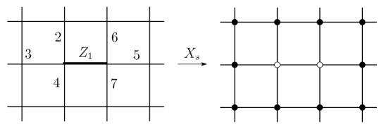
The action of the error can be written as $Z_{1}|\Psi\rangle$. If we apply the star operator around $Z_{1}$ on the square lattice, we obtain a pair of the outputs with the negative value $-1$ as

$$X_{1}X_{2}X_{3}X_{4}Z_{1}|\Psi\rangle=-Z_{1}X_{1}X_{2}X_{3}X_{4}|\Psi\rangle=-Z_{1}|\Psi\rangle$$ (72)

$$X_{1}X_{5}X_{6}X_{7}Z_{1}|\Psi\rangle=-Z_{1}X_{1}X_{5}X_{6}X_{7}|\Psi\rangle=-Z_{1}|\Psi\rangle,$$ (73)

where we use anti commutation as $Z_{1}X_{1}=-X_{1}Z_{1}$. On the other hand, the flip error by $X$ can be detected by the plaquette operator on the dual lattice. At least, we can identify the location of the endpoints on the error chains denoted as $\partial E$ and $\partial E^{*}$.

We do not know the exact shape of the error chains $E$ and $E^{*}$. We must remove the effect of the errors on the torus only by use of the outputs of the check operators, error syndrome, $\partial E$ and $\partial E^{*}$. Thus we must infer the original state from the damaged one with negative outputs on several sites and plaquettes. To remove the damage signaled by the negative eigenvalues, we consider to apply additional actions of the product of the Pauli operators. This procedure is to simply connect two endpoints of the error chains we can know. The additional actions with the original error chains can conform closed loops. The resulting effects are trivial on the codespace. However, if nontrivial, we can no longer restore the original quantum state.

In order to make the resulting effect trivial, we have to choose additional actions while inferring the same homology class as the logical operators encoding the original information only with the knowledge of the endpoints. The best way (optimal procedure) is to find out the most probable homology class. It reads, if we define $P(\bar{E},\bar{E}^{*}|\partial E,\partial E^{*})$ as the probability of the inferred homology class $\bar{E}$ and $\bar{E}^{*}$ conditioned on $\partial E$ and $\partial E^{*}$,

$$\mathrm{max}_{\bar{E},\bar{E}^{*}}P(\bar{E},\bar{E}^{*}|\partial E,\partial E^{*}),$$ (74)

where $\bar{E}$ and $\bar{E}^{*}$ denote the possible homology class of the error chains. Observant readers begin to recognize an existence of the limitation of the above procedure. First, increase of the error probability $p$ might allow the possibility of the non-contractible error chains wounding the torus. If we prepare sufficient large torus, this is not expected to occur as $\sim p^{L}\to 0$. As this instance, the system size $L$ becomes larger, tolerance of the surface code against the error can be enhanced. However, if $p$ is not small, we can not always determine the same homology class with the error chains among several candidates, since we tend to infer the wrong homology class due to the existence of long and many error chains. The connections among the original error chains and the additional actions would conform a long loop wounding the torus if $p$ exceeds a threshold. Such an accuracy threshold actually exists and can be determined by special technique developed in the theory on the phase transition in statistical mechanics. In practice, the ideal error correction by inferring the most probable homology class of the error chains should be too harmful due to computational costs. We need to take some approximate technique in a moderate time. However, if we can, it is important to estimate the optimal error threshold in order to reveal the theoretical limitation of the surface code.

In the following, we construct the statistical-mechanical model to pave the way to analytically estimate the optimal accuracy threshold.

3.2.2 Probability of error chains

Notice that our task is to elucidate the macroscopic property in the error correcting procedure, not actual many-body quantum system. The outputs of the measurements of the check operators and the procedure of the application of additional actions based on the inferred homology class are classical. Although we deal with the problem on the quantum error correction, all the methods we employ here may not be quantum.

The error on each qubits occur in the probabilistic manner. Therefore let us construct a probabilistic model of the quantum error correction on the torus. In order to deal with the asymptotic behavior of the error pattern and inferred chains in the infinite-number limit, we use the most suited technique, statistical mechanics. Statistical mechanics starts from constructing a probabilistic model in the microscopic level. Following the concept of the large deviation principle, we take an infinite number limit of the system size in order to predict the deterministic macroscopic behavior.

Now we take the simple case with uncorrelated errors. We can separately deal with the flip and phase errors. For simplicity, hereafter we consider only the phase errors given by the actions of $Z$ on the original square lattice.

From the knowledge of endpoints $\partial E$, error syndrome, we have to infer the most likely homology class of the error chains, while considering any reasonable choices.

For instance, let us consider the reasonable connections $E^{\prime}$ between each pair of the endpoints $\partial E$ as in Fig. 10.

Figure 10: Reasonable connections $E^{\prime}$ inferred from $\partial E$. For transparency, the square lattice is depicted by the dotted lines.

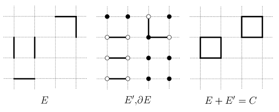
As a result, we can make contractible loops denoted by $C$ on the square lattice. Then the reasonable chains $E^{\prime}$ inferred from $\partial E$ are in an equivalent class with the error chains. However there are several cases to infer non-equivalent class with the error chains as in Fig. 11.

Figure 11: Failure of inference of the equivalent class with $E$. The wounding chain by the product of $Z$ yields $Z_{t}$ denoted by $(k_{1},k_{2},k_{3},k_{4})=(0,1,0,0).$

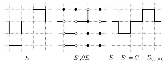
By use of the Bayes theorem, we consider to evaluate the probability to infer the equivalent homology class with the original error chains conditioned on those endpoints as follows

$$P(\bar{E}|\partial E)=\frac{P(\partial E|\bar{E})P(\bar{E})}{\sum_{k_{1},k_{2},k_{3},k_{4}}P(\partial E|\bar{E}+D_{k_{1},k_{2},k_{3},k_{4}})P(\bar{E}+D_{k_{1},k_{2},k_{3},k_{4}})},$$ (75)

where $D_{k_{1},k_{2},k_{3},k_{4}}$ denotes the logical operator. The equivalent class is given simply by $D_{0,0,0,0}=\phi$. If we infer the different class denoted by $(k_{1},k_{2},k_{3},k_{4})\neq(0,0,0,0)$, the error correction fails. We assume that the prior probability for the homology classes is uniform, namely $P(\partial E)=1/16$, since we encode various combinations of the different homology classes. Our task is to consider $P(\partial E|\bar{E})$, which is the probability to generate the endpoints of the specific error chains. Let us first evaluate the probability for the specific error chains. The error chains are generated following the independently identical distribution as

$$P(E) = \prod_{\langle ij\rangle}p^{\frac{1+\tau^{E}_{ij}}{2}}(1-p)^{\frac{1-\tau^{E}_{ij}}{2}}$$ (76)

$$= \left\{p(1-p)\right\}^{\frac{N_{B}}{2}}\prod_{\langle ij\rangle}\left(\frac{p}{1-p}\right)^{\frac{\tau^{E}_{ij}}{2}},$$

where $\tau^{E}_{ij}$ represents the error chains and takes $\pm 1$ ($\tau^{E}_{ij}<0$, when $(ij)\in E$). Here we introduce the expression of the exponential form as in the case for the spin glass and obtain

$$P(E)=\prod_{\langle ij\rangle}\frac{\exp(K_{p}\tau^{E}_{ij})}{2\cosh K_{p}}.$$ (77)

Notice that $K_{p}$ is minus of the original definition in the spin glass. Then, in order to evaluate $P(\partial E|\bar{E})$, we sum over all the possible configurations $E^{\prime}=E+C$ of the error chains sharing the endpoints. We reach

$$P(\partial E|\bar{E})\propto\sum_{C}\prod_{\langle ij\rangle}\exp(K_{p}\tau^{E}_{ij}\tau^{C}_{ij}),$$ (78)

where the summation is taken over all the possibilities of $C$ and the product is over all the edges. We use the same indicators as $\tau_{ij}^{E}$ for $C$.

This probability tells us how to proceed the error correction. We simply perform the connection of the endpoints in the stochastic manner. If we know $p$ in advance, it is better to set the same value. Otherwise we have

$$P_{K}(\partial E|\bar{E})\propto\sum_{C}\prod_{\langle ij\rangle}\exp(K\tau^{E}_{ij}\tau^{C}_{ij}).$$ (79)

The parameter $K$ stands for the importance/preference to choose the reasonable choice in the connection of the endpoints. For instance, in the case with $K\to\infty$, $E^{\prime}$ with the minimum length are preferred. The performance of the error correction depends on the value of $K$.

The loop constraints $\prod_{(ij)}\tau_{ij}^{C}=1$ allow to use another expression by the Ising variables $\tau_{(ij)}^{C}=S_{i}S_{j}$. By use of this expression, we can find that $P(\bar{E})$ is written by the partition function of the $\pm J$ Ising model as

$$P_{K}(\partial E|\bar{E})\propto Z(K;\{\tau_{ij}\})=\sum_{\{S_{i}\}}\prod_{\langle ij\rangle}\mathrm{e}^{K\tau^{E}_{ij}S_{i}S_{j}},$$ (80)

where $\tau^{E}_{ij}$ is the sign of the random coupling in context of spin glasses. Each of the random couplings follows the distribution function of the error chains $P(E)$. Notice that, in this case, $p$ denotes the density of the antiferromagnetic interactions. Therefore the problem to identify the error threshold of the surface code is reduced into evaluating the quantity related with the partition function of the simple spin-glass model, the $\pm J$ Ising model on the square lattice. If we increase $p$, the spin-glass system will be not rigid against thermal fluctuations, since the ferromagnetic order decays. Similarly, in the surface code, increase of $p$ is expected to lead the error correction to be unfeasible. These analogous implies the existence of a fascinating relationship between the phase transition in the spin glass and the error threshold in the surface code.

In order to more clearly see this connection between statistical mechanics and quantum error correction, we show a schematic picture of the phase diagram for the $\pm J$ Ising model on the square lattice as in Fig. 12.

Figure 12: Phase diagram of the $\pm J$ Ising model. The figure is depicted by the same symbols in Fig. 4. In the two-dimensional case, the absence of the spin-glass phase has been partially proved and supported by numerical simulations. [23].

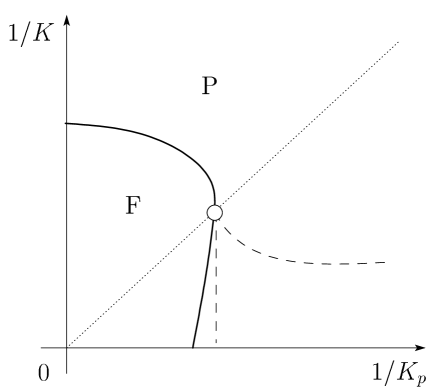
In the low-temperature region with a relatively small $p$, the ferromagnetic ordered phase can be observed. It means that the order of the Ising spins exists and suppresses the fluctuation of the domain walls (boundaries between different signed spins). Let us consider to evaluate $P_{K}(\bar{E}|\partial E)$ in the ferromagnetic phase. We rewrite the probability as, in terms of the free energy of the spin glass,

$$P_{K}(\bar{E}|\partial E)=\frac{1}{1+\sum_{\{k_{i}\}}\exp(-K\Delta F_{k_{1},k_{2},k_{3},k_{4}})}.$$ (81)

Here the difference of the free energy $\Delta F_{k_{1},k_{2},k_{3},k_{4}}$ is given as

$$\Delta F_{k_{1},k_{2},k_{3},k_{4}}=F(K;\{\tau_{ij}\})-F(K;\{\tau_{ij}\tau^{D_{k_{1},k_{2},k_{3},k_{4}}}_{ij}\}),$$ (82)

where we use $K$ instead of $\beta$ as

$$F(K;\{\tau_{ij}\tau^{D_{k_{1},k_{2},k_{3},k_{4}}}_{ij}\})=-\frac{1}{K}\log Z(K;\{\tau_{ij}\tau^{D_{k_{1},k_{2},k_{3},k_{4}}}_{ij}\}).$$ (83)

In context of statistical mechanics, the logical operator $D_{k_{1},k_{2},k_{3},k_{4}}$ is interpreted as the induction of the antiferromagnetic interactions along the non-contractible loop as $\{\tau_{ij}\tau^{D_{k_{1},k_{2},k_{3},k_{4}}}_{ij}\}$. In the ferromagnetic phase, such a long boundary of antiferromagnetic interactions yields a crevice with the same scale as the inducted loop in the ordered spins. Therefore the free energy difference should become $\sim\mathcal{O}(L)$. As a result, the probability to infer the equivalent homology class with the original error chains is asymptotically, in the limit of $L\to\infty$

$$P_{K}(\bar{E}|\partial E)\to 1.$$ (84)

This means that the error correction is feasible.

On the other hand, in a high temperature and for not a small $p$, namely the paramagnetic phase, the order of the spins is destroyed. The vast number of islands of the different-signed spins can exist and the boundaries fluctuate. The free-energy difference becomes zero, and thus we reach.

$$P_{K}(\bar{E}|\partial E)\to 1/16.$$ (85)

This means that the error correction is infeasible. Therefore the locations of the critical points of the spin-glass model identify the error thresholds of the surface code. In particular, the optimal threshold is located on the special critical point along the Nishimori line, namely multicritical point [7, 22], since it is at the most right side in the phase diagram. In other words, if we know the precise value of $p$, it is easier to correct the errors in the logical qubits.

3.3 Analyses on accuracy thresholds for surface code

In general, the problem on finite-dimensional spin glasses is intractable. However recent development in theory of this realm enables us to estimate a precise location of the critical point in several spin glasses. In the following section, we introduce such a specialized theory in detail.

3.3.1 Duality analysis: simple case

The situation that no systematic analytical methods attacking the problems on the critical phenomena in finite-dimensional spin glasses have been changed since a recent development in the spin-glass theory. It enables us to estimate the precise value of the special critical point especially on the Nishimori line, which corresponds to the optimal error threshold [24, 25, 26, 27]. The method as shown below is based on the duality, which can identify the location of the critical point especially on two-dimensional spin systems [28, 29]. Let us review the simple case of the Ising model.

The duality is a symmetry argument by considering the low and high-temperature expansions of the partition function. As a result, we can obtain a simple relation between two different temperatures through the partition function as

$$Z(K)=\Lambda Z(K^{*}),$$ (86)

where $K^{*}$ denotes the dual coupling constant related with the original one $K$. The coefficient $\lambda$ will be an important quantity below.

We here deal with the case for the Ising model on the square lattice, whose partition function is given as, through the Hamiltonian (20),

$$Z(K)=\sum_{\{S_{i}\}}\prod_{\langle ij\rangle}\exp(KS_{i}S_{j}),$$ (87)

where the product is taken over all the nearest neighboring pairs on the square lattice. The original formulation of the duality analysis is based on a relatively painful calculation [28]. We here show a much simpler version given by a simple Fourier transformation for the local part of the Boltzmann factor [29].

We define the edge Boltzmann factor as

$$x_{\phi}(K)=\exp(K\cos\pi\phi),$$ (88)

where we use another binary variable as $\phi=0$ and $1$, instead of the Ising spin. In addition, we apply the binary Fourier transformation to this quantity, called as the dual edge Boltzmann factor,

$$x^{*}_{k}(K)=\frac{1}{\sqrt{2}}\sum_{\phi=0,1}x_{\phi}\exp(\mathrm{i}\pi k\phi)=\frac{1}{\sqrt{2}}\left(\mathrm{e}^{K}+\mathrm{e}^{-K}\cos\pi k\right).$$ (89)

Then we find that the partition function can be written in two ways by both of the edge Boltzmann factors. First, the partition function is simply expressed by the original Boltzmann factor as

$$Z(K)=\sum_{\{\phi_{i}\}}\prod_{\langle ij\rangle}x_{\phi_{ij}}(K),$$ (90)

where $\phi_{ij}=\phi_{i}-\phi_{j}$. The difference between $\phi_{i}$ and $\phi_{j}$ is taken in order from left to right and from top to bottom. Inserting the inverse Fourier transformation of the dual edge Boltzmann factor yields another expression of the partition function

$$Z(K)=\left(\frac{1}{\sqrt{2}}\right)^{N_{B}}\sum_{\{\phi_{i}\}}\sum_{\{k_{ij}\}}\prod_{\langle ij\rangle}x^{*}_{k_{ij}}(K)\mathrm{e}^{\mathrm{i}k_{ij}(\phi_{i}-\phi_{j})}.$$ (91)

Here let us perform the summation over $\{\phi_{i}\}$ by considering the adjacent edges. We concentrate on the particular site $0$ and then find that the exponential term can be factorized and the summation can be taken independently as

$$\sum_{\phi_{0}=0,1}\mathrm{e}^{\mathrm{i}(-k_{10}-k_{20}+k_{03}+k_{04})\phi_{0}}=2\delta(k_{10}+k_{20}-k_{03}-k_{04}\equiv 0~{}(\mathrm{mod}~{}2)).$$ (92)

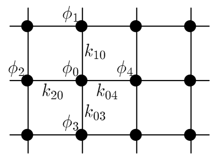
We describe adjacent edges to the particular site $0$ as in Fig. 13.

Figure 13: Description of the terms appearing in Eq. (92)

In order to remove the terms of the Kronecker’s delta functions, we employ another binary variable as

$$k_{10} = \phi^{*}_{1}-\phi^{*}_{2}$$ (93)

$$k_{20} = \phi^{*}_{2}-\phi^{*}_{3}$$ (94)

$$k_{03} = \phi^{*}_{4}-\phi^{*}_{3}$$ (95)

$$k_{04} = \phi^{*}_{1}-\phi^{*}_{4}.$$ (96)

We set these new variables $\{\phi^{*}_{i}\}$ on each plaquette on the square lattice, namely each site on the dual one. The resultant expression of the partition function is

$$Z(K)=\sum_{\{\phi^{*}_{i}\}}\prod_{\langle ij\rangle}x^{*}_{\phi^{*}_{ij}}(K),$$ (97)

where $\phi^{*}_{ij}\equiv\phi^{*}_{i}-\phi^{*}_{j}$. This fact leads us to the double expressions with the different arguments as

$$Z(x_{0}(K),x_{1}(K))=Z(x^{*}_{0}(K),x^{*}_{1}(K)).$$ (98)

To reduce the number of the arguments, we normalize the partition function by the principal edge Boltzmann factors $x_{0}(K)$ and $x_{0}^{*}(K)$.

$$\left\{x_{0}(K)\right\}^{N_{B}}z(u_{1}(K))=\left\{x^{*}_{0}(K)\right\}^{N_{B}}z(u^{*}_{1}(K)),$$ (99)

where $z$ is the normalized partition function $z(u_{1})=Z/\{x_{0}(K)\}^{N_{B}}$ and $z(u^{*}_{1})=Z/\{x^{*}_{0}(K)\}^{N_{B}}$. We explicitly obtain $u_{1}(K)=x_{1}(K)/x_{0}(K)=\exp(-2K)$ and $u_{1}^{*}(K)=x^{*}_{1}(K)/x^{*}_{0}(K)=\tanh K$. It reads, if we set the dual coupling as $\exp(-2K^{*})=\tanh(K)$,

$$\left\{x_{0}(K)\right\}^{N_{B}}z(u_{1}(K))=\left\{x^{*}_{0}(K)\right\}^{N_{B}}z(u_{1}(K^{*})).$$ (100)

Therefore we find that the partition function for the Ising model has symmetry between two different temperatures. This is the duality. The coefficient $\Lambda$ is also obtained as

$$\Lambda=\left(\frac{x^{*}_{0}(K)}{x_{0}(K)}\right)^{N_{B}}=\left\{\frac{1}{\sqrt{2}}\left(1+\exp(-2K)\right)\right\}^{N_{B}}.$$ (101)

The well known duality relation $\exp(-2K^{*})=\tanh K$ can identify the exact location of the critical point by equating $K=K^{*}$. The critical point is estimated as $K_{c}=\ln(1+\sqrt{2})/2=0.440686794\cdots$. Interestingly, the coefficient $\Lambda$ becomes unity at the critical point. We use this property as a priori assumption for the analysis on the critical point for spin glasses.

3.3.2 Duality analysis: spin glass

The replica method, which is often used in theoretical studies on spin glasses, allows to generalize the duality analysis to spin glasses [24, 25]. Let us consider the duality for the replicated partition function as $[Z^{n}(K;\{\tau_{ij}\}]$. In this case, the multiple binary Fourier transformation defines the dual edge Boltzmann factor as

$$x^{*}_{k_{1},k_{2},\cdots,k_{n}}(K_{p},K)=\left(\frac{1}{\sqrt{2}}\right)^{n}\sum_{\phi_{1},\phi_{2},\cdots,\phi_{n}}x_{\phi_{1},\phi_{2},\cdots,\phi_{n}}(K_{p},K)\mathrm{e}^{\mathrm{i}\sum_{i=1}^{n}k_{i}\phi_{i}},$$ (102)

where the original edge Boltzmann factor is given by the configurational average of the $n$-replicated $\pm J$ Ising model,

$$x_{\phi_{1},\phi_{2},\cdots,\phi_{n}}(K_{p},K)=\frac{1}{2\cosh K_{p}}\left\{\mathrm{e}^{-K_{p}+K\sum_{i=1}^{n}\cos\pi\phi_{i}}+\mathrm{e}^{K_{p}-K\sum_{i=1}^{n}\cos\pi\phi_{i}}\right\}.$$ (103)

Notice that the definition of $p$ is the density of the antiferromagnetic interactions here to analyze the accuracy threshold for the surface code. They leads us to the double expression of the replicated partition function as, in a similar way to the above simple case,

$$\{x_{0}(K_{p},K)\}^{N_{B}}z(u_{1}(K_{p},K),u_{2}(K_{p},K),\cdots)$$

$$=\{x^{*}_{0}(K_{p},K)\}^{N_{B}}z(u^{*}_{1}(K_{p},K),u^{*}_{2}(K_{p},K),\cdots),$$ (104)

where the subscript of $u_{k}$ and $u_{k}^{*}$ stands for the number of anti-parallel pair among $n$ replicas on each edge. We restrict ourselves to the case to analyze the location of the multicritical point, namely $K=K_{p}$ on the Nishimori line.

Unfortunately we cannot replace $u^{*}_{k}(K,K)$ by $u_{k}(K^{*},K^{*})$ even after normalization as the above case for the Ising model, since the replicated partition function is multivariable. Nevertheless we can estimate the location of the multicritical point even without the ordinary procedure of the duality. We here put a priori assumption that $x_{0}(K,K)=x^{*}_{0}(K,K)$ at the critical point, implying the coefficient of the double expressions of the replicated partition function should be unity. According to this assumption, we take the limit $n\to 0$ of the equation along the replica method and thus obtain

$$-p\log p-(1-p)\log(1-p)=\frac{1}{2}\log 2.$$ (105)

The solution is $p_{c}=0.1100\cdots$. We thus conclude that the accuracy threshold is estimated as $p_{c}=0.1100\cdots$. Strictly speaking, this analysis is not exact. In practical, the precision of the above result has been confirmed to be satisfiable by supports from numerical simulations. In addition to such numerical validations, the following theoretical refinement of the method to identify the multicritical point have been considered.

3.3.3 Duality analysis with real-space renormalization

As above mentioned, the ordinary duality analysis hampers since the replicated partition function was multivariable. Thus we rely on the assumption that $x_{0}(K,K)=x^{*}_{0}(K,K)$ would give the location of the critical point. We here sketch the relationship between the double expressions of the replicated partition function as the curves of the relative Boltzmann factors $u_{k}(K,K)$ and $u^{*}_{k}(K,K)$ on the two-dimensional space for simplicity, although those are correctly in a hyper space as in Fig. 14.

Figure 14: Relative Boltzmann factors of the replicated partition function (Projection onto two dimensions). The high-temperature limit is given by P, while the low-temperature limit is $F$. The solid curve represents the original relative Boltzmann factor. The dashed curve denotes the dual relative Boltzmann factor.

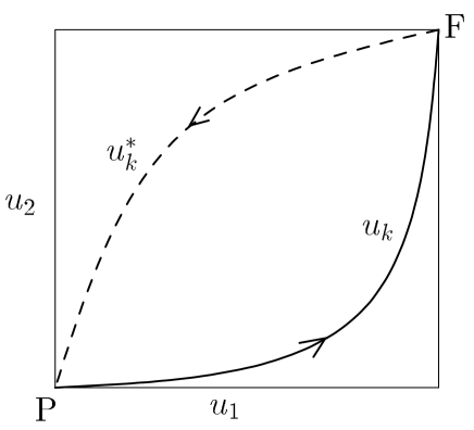
The thick curve denotes the relative Boltzmann factor $u_{k}(K,K)$ and the dashed one represents the dual one $u^{*}_{k}(K,K)$. When the temperature increases, the representative point of the replicated partition function moves from P (the high-temperature limit) to F (the low temperature limit) along the thick curve. On the other hand, the dual representative point goes inversely along the dashed curve. These features have been shown rigorously and imply the existence of the duality relation for the temperature [30] . If two curves become completely coincident with each other, we then obtain a relation implying $u^{*}_{k}(K,K)=u_{k}(K^{*},K^{*})$. Solving this relation, we can obtain the duality relation for different temperatures as the case of the Ising model. In spin glasses, they do not overlap.

We import another piece of the theories in statistical mechanics, the real-space renormalization group analysis. Most of the problems on statistical mechanics are tractable since the degrees of freedom are highly correlated. Often we employ a trick to map the original problem into much simpler problem with a recursive structure by use of some approximation. As in Fig. 15, we trace over a part of spins on the square lattice.

Figure 15: Real-space renormalization. In this instance, a limited number of spins are summed, and the remaining ones construct another square lattice with multiple-body interactions.

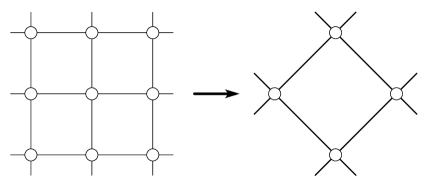
Repeating this procedure while omitting the generated multi-body interactions (approximation), we construct the renormalization group in the form of the recursion

$$K_{n}=R(K_{n-1}),$$ (106)

where $K_{n}$ is the renormalized coupling constant after $n$ steps. By use of the renormalization group analysis, we describe flow of the renormalized coupling constant in $K$ space. The flow usually terminates two fixed points representing the ordered and disordered phase, while being divided by an unstable fixed point, which is the critical point. The precision to represent the original behavior in the model is dependent on the approximation in construction of the renormalization group. We generalize this procedure into the relative Boltzmann factors $\{u_{k}(K,K)\}$ and $\{u^{*}_{k}(K,K)\}$. The flow can be depicted in the hyper space of $\{u_{k}(K,K)\}$ as in Fig. 16. Similarly to the above simple case, the renormalization flow goes toward two fixed points P and F.

Figure 16: Relative Boltzmann factors of the replicated partition function and their renormalization flow (Projection onto two dimensions). The dotted arrows depict the renormalization flow starting from several points on both of the relative Boltzmann factors. The internal curves denote the renormalized relative Boltzmann factors. The bold curve describes the sufficiently renormalized relative Boltzmann factors with the unstable fixed point as the case with a single variable in the partition function.

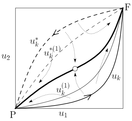
The unstable fixed point $C$ would be located between the original and dual relative Boltzmann factors, since they do not overlap but have a common critical point. The renormalization flow starts from both of the relative Boltzmann factors and once moves to the unfixed point. After several renormalization steps, the flow goes to two fixed points. That means that, if we conduct one step of the renormalization for each point on the original and dual relative Boltzmann factors, we observe both of the renormalized curves get close to each other as in Fig. 16. The sufficient steps of the renormalization makes both of the curves into a common thick curve capturing the unfixed point, namely the multicritical point. As far as possible, we desire to estimate the location of the critical point precisely. Then, let us consider to trace the partial spins without any approximations. For example, in the case on the square lattice, we define the cluster Boltzmann factor $x_{k}^{(s)}(K,K)$, where the subscript $k$ denotes the configuration of the edge (white-colored) spins and $s$ expresses the size of the cluster in Fig. 17. When $k=0$, all the edge spins are in up directions.

Figure 17: Clusters for duality with renormalization. The white circles denote edge spins whose configuration is represented by $k$, and the black ones are to be summed.

We sum over the internal (black-colored) spins in order to perform the renormalization without approximation. It is difficult to perform the sufficient step of the renormalization without any approximation. Remember that we can estimate the relatively correct value of the multicritical point even without the renormalization. Therefore we propose a systematic way to improve precision of the location of the multicritical point. We employ the following equation to estimate the location of the multicritical point,

$$x_{0}^{(s)}(K,K)=x_{0}^{*(s)}(K,K).$$ (107)

The equality for $s=0$ (edge) reproduces the case without renormalization as $p^{(0)}_{c}=0.1100$ [24, 25]. If we increase the size of the used cluster, we can systematically approach the exact solution for the location of the multicritical point of the $\pm J$ Ising model as $p^{(1)}_{c}=0.1093$ and $p^{(2)}_{c}=0.1092$.

If we remove the condition of the Nishimori line $K_{p}=K$, we can describe the phase boundary for spin glasses by

$$x_{0}^{(s)}(K_{p},K)=x_{0}^{*(s)}(K_{p},K).$$ (108)

By use of this equation, we can obtain the precise results for the phase boundary in the higher temperature region than the Nishimori line and the whole phase boundary of the diluted Ising model [26, 27].

3.3.4 Other cases

Not only the surface code, several quantum error correcting codes are found to possess the connection with the spin-glass models. Although we omit their detailed explanations, we look over the recent results in short below. We restrict ourselves to the case in which the duality analysis have predicted the accuracy threshold.

First, we simply mention the cases by other arrangement of physical qubits in the surface code than the square lattice, say triangular and hexagonal lattices. The accuracy threshold for both of the lattices can be given as $p_{c}=0.164\cdots$ (triangular) and $p_{c}=0.067\cdots$(hexagonal) [27]. Recently, another type of the surface code with more computational capability have been developed, color code. Also in the case of the color code, we prepare the arrangement of the physical qubits on each unit triangle on the triangular lattice or Union-Jack lattice as in Fig. 18. [31, 32]. The color code on the Union-Jack lattice implements the whole Clifford group of unitary gates generated by the Hadamard gate, the $\{\pi/8\}$ gate, and the controlled-NOT gate, although that on the triangular lattice can not employ the $\{\pi/8\}$ gate. It means that both of the color codes have the wider computational capability than that of the Pauli group.

Figure 18: Color code on the triangular and Union-Jack lattices.

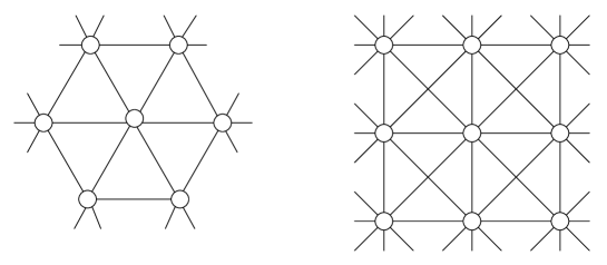
The corresponding statistical mechanical model has three-body interactions differently from the above surface code. The quenched random interaction then represents the error arising on the physical qubits on the unit triangles. Here the duality analysis can estimate the accuracy thresholds for both of the color codes as $p_{c}=0.1096-8$ (triangular) and $p_{c}=0.1092-3$ [33]. Interestingly, the advantage of the computational capability does not spoil the robustness of the error correction.

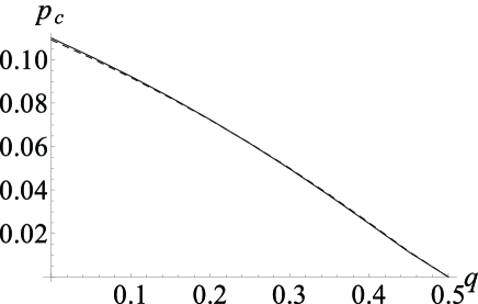
In addition, the practical errors in implementation of the quantum system are not only on the computational basis. Lack of the physical qubits is also likely to occur. Recently, Stace et al. have proposed a modified scheme of the surface code to protect the logical quantum state from both type of the errors, namely from decoherence and lack of the physical qubits [34, 35]. Then the corresponding statistical mechanical model becomes the diluted version of the $\pm J$ Ising model. We can identify the locations of the optimal thresholds depending on the ratio of the loss of the physical qubits $q$ as in Fig. 19 [36]. The detailed values are shown in Table 3.3.4. As shown in Table 3.3.4 and Fig. 19, the decay of the robustness, depending on increase of $q$, of the surface code against the flip/phase errors can be observed. This behavior can be interpreted as the decay of the ferromagnetic order due to the dilution of the interactions.

Optimal thresholds given by the duality analyses with $s=0$, $1$, and $2$ clusters for the uncorrelated case. $q$ $p_{c}$ ($s=0$) $p_{c}$ ($s=1$) $p_{c}$ ($s=2$) $0.00$ $0.11003$ $0.10928$ $0.10918$ $0.10$ $0.09240$ $0.09196$ $0.09189$ $0.20$ $0.07245$ $0.07235$ $0.07233$ $0.30$ $0.04984$ $0.05004$ $0.05009$ $0.40$ $0.02462$ $0.02492$ $0.02500$ $0.45$ $0.01155$ $0.01174$ $0.01179$

Figure 19: Decay of the robustness due to loss of the physical qubits. The solid curve expresses the results by the duality with $s=0$ and the dashed curve denotes those with $s=1$, while both of them are mostly overlapping in this scale.

3.3.5 Depolarizing channel

Before closing this section, we add another example on the quantum error correction related with statistical mechanics. We discussed the case without correlation of both of the flip and phase errors for simplicity. It is straightforward to generalize the above procedure for the depolarizing channel case such that the error probabilities are equalized as $p_{X}=p_{Y}=p_{Z}=p/3$. In this case, the corresponding statistical mechanical model becomes a little bit different one from the $\pm J$ Ising model. We can no longer independently deal with both of the errors. Let us first evaluate the probability for the specific error chains. The error chains are generated following the distribution function as

$$P(E,E^{*}) = \prod_{\langle ij\rangle}\left(\frac{p}{3}\right)^{\frac{1+\tau^{E}_{ij}}{4}+\frac{1+\tau^{E^{*}}_{ij}}{4}+\frac{1+\tau^{E}_{ij}\tau^{E^{*}}_{ij}}{4}}(1-p)^{\frac{1-\tau^{E}_{ij}}{4}+\frac{1-\tau^{E^{*}}_{ij}}{4}+\frac{1-\tau^{E}_{ij}\tau^{E^{*}}_{ij}}{4}}$$ (109)

$$\propto \left(\frac{p}{3(1-p)}\right)^{\frac{\tau^{E}_{ij}}{4}+\frac{\tau^{E^{*}}_{ij}}{4}+\frac{\tau^{E}_{ij}\tau^{E^{*}}_{ij}}{4}}.$$

We again use the expression of the exponential form as in the case for the spin glass and obtain

$$P(E,E^{*})\propto\prod_{\langle ij\rangle}\exp(K_{d}\tau^{E}_{ij}+K_{d}\tau^{E^{*}}_{ij}+K_{d}\tau^{E}_{ij}\tau^{E^{*}}_{ij}).$$ (110)

Notice that $\exp(-4K_{d})=3(1-p)/p$. Similarly, the problem is to identify the singularity of the following the probability through the partition function of a spin glass

$$P_{K}(\partial E,\partial E^{*}|\bar{E},\bar{E}^{*})$$

$$\quad\propto\sum_{{}_{S_{i},S_{i}^{*}}}\prod_{\langle ij\rangle}\exp(K\tau^{E}_{ij}S_{i}S_{j}+K\tau^{E^{*}}_{ij}S^{*}_{i}S^{*}_{j}+K\tau^{E}_{ij}\tau^{E^{*}}_{ij}S_{i}S_{j}S^{*}_{i}S^{*}_{j}),$$

where the quenched random coupling obeys the distribution function $P(E,E^{*})$ . This model is regarded as a spin-glass version of the $4$-state Potts model.

The duality analysis can be performed for this statistical-mechanical model in order to estimate the optimal thresholds [37]. In addition, we can apply the modified scheme to circumvent the effects due to loss of the physical qubits proposed by Stace et al. [36]. We list the results for the depolarizing channel in Table 3.3.5.

Results for the correlated case (depolarizing channel) $p_{X}=p_{Z}=p_{Y}=p/3$. $q$ $p_{c}$ ($s=0$) $p_{c}$ ($s=1$) $0.00$ $0.18929$ $0.18886$ $0.10$ $0.16025$ $0.15985$ $0.20$ $0.12690$ $0.12656$ $0.30$ $0.08844$ $0.08819$ $0.40$ $0.04454$ $0.04440$ $0.45$ $0.02121$ $0.02114$

4 Quantum annealing and beyond

The second part of this chapter, we introduce another application of statistical mechanics in context of quantum computation. As in the other chapter, by use of the analogy of simulated annealing (SA) developed in statistical mechanics, a generic algorithm intended for solving optimization problems by use of quantum nature, quantum annealing (QA), has been studies since its proposal. In SA, we make use of thermal, classical, fluctuations to employ a stochastic search for the desired lowest-energy state, which corresponds to the optimal solution, by allowing the system to hop from state to state over intermediate energy barriers. In QA, by contrast, we introduce non-commutative operators as artificial degrees of freedom of quantum nature in order to induce quantum fluctuations. The most typical procedure of QA is performed by adiabatic control of quantum fluctuations, say quantum adiabatic computation (QAC). The adiabatic theorem guarantees that an sufficient slow time evolution would let the system closely follow the instantaneous ground state. Therefore, starting from an initial trivial ground state, we can reach a nontrivial one by slowly controlling quantum fluctuations. However, in a practical sense, we desired to perform the procedure to find the answer of the optimization problem as fast as possible. The adiabatic control to efficiently obtain the optimal solution takes a characteristic time related with the energy gap between the first excited state and the lowest one during its procedure. The problems with closure of the energy gap are difficult to be solved in a moderate time by QAC. Unfortunately, as far as we know, the typical difficult problems in classical computation involves the exponential closure of the energy gap by increase of the problem size.

In this chapter, we show several trials to overcome the bottleneck of quantum adiabatic computation by use of statistical mechanics. We use formal similarities between SA and QAC in order to import several developments in statistical mechanics. In both methods, we have to drive the system slowly and carefully to control the strengths of thermal or quantum fluctuations. The idea behind quantum adiabatic computation is to keep the system close to the instantaneous ground state of a quantum system. This is analogous to the protocol of SA, in which one tries to make the system keep quasi-equilibrium state. It is indeed possible to make this analogy more transparent by a precise formulation, from which a fascinating technique to be expected to improve the performance of QAC can be proposed.

4.1 Quantum adiabatic computation: short review

Let us briefly review the procedure of the most typical QA, namely QAC, before importing theory of statistical mechanics to quantum computation. In QA, we introduce a non-commutative operator to drive the system by quantum nature as

$$H(t)=f(t)H_{0}+\left(1-f(t)\right)H_{1},$$ (112)

where $H_{0}$ is the classical Hamiltonian consisting of diagonal elements, which express the cost function. Here $f(t)$ is assumed to be a monotonically increasing function satisfying $f(0)=0$ and $f(T)=1$. For instance, $f(t)=t/T$, where $T$ denotes the computation time for QAC. The quantum annealing starts from a trivial ground state of $H_{1}$, which is often chosen to be a uniform linear combination of the computational basis as $|\Psi(0)\rangle=|\sigma\rangle/\sqrt{N}$. Let us deal with only the discrete combinatorial optimization problems, which are simply termed as the optimization problem below. Most of the optimization problem can be expressed by the spin-glass Hamiltonian. In order to explain the procedure of QAC in detail, we consider to find the ground state of the simple spin-glass model as used before, namely the random-bond Ising model,

$$H_{0}=-\sum_{\langle ij\rangle}J_{ij}\sigma_{i}^{z}\sigma_{j}^{z},$$ (113)

where the summation is taken over all the nearest-neighboring pairs of the Ising spins. We take the computational basis of the eigenstates of the Ising variables to represent the instantaneous state as $|\Psi(t)\rangle=|\sigma_{1}^{z},\sigma_{2}^{z},\cdots,\sigma_{N}^{z}\rangle$. The transverse-field operator is often used as quantum fluctuations for implementing QAC for the spin-glass model

$$H_{1}=-\Gamma_{0}\sum_{i=1}^{N}\sigma_{i}^{x},$$ (114)

where $\Gamma_{0}$ is the strength of the transverse field. The whole Hamiltonian of QAC (although widely used for QA) thus becomes

$$H(t)=f(t)\sum_{\langle ij\rangle}J_{ij}\sigma^{z}_{i}\sigma_{j}^{z}+\left(1-f(t)\right)\Gamma_{0}\sum_{i=1}^{N}\sigma^{x}_{i}.$$ (115)

The ground state of the transverse-field operator $H_{1}$ is trivially given by a uniform linear combination as $\sum_{\{\sigma\}}|\sigma\rangle/\sqrt{2}^{N}$. For a sufficiently large $T$, the adiabatic theorem guarantees that the instantaneous state at time $t$, $|\Psi(t)\rangle$, is very close to the instantaneous ground state implying $|0(t)\rangle$, $\langle 0(t)|\Psi(t)\rangle\approx 1$, when the instantaneous ground state $|0(t)\rangle$ is non-degenerate. The condition for $|0(t)\rangle$, $\langle 0(t)|\Psi(t)\rangle 1-\epsilon^{2}(\epsilon\ll 1)$ to hold is given by

$$\frac{\mathrm{max}\left|\langle 1(t)|\frac{dH(t)}{dt}|0(t)\rangle\right|}{\mathrm{min}\Delta^{2}(t)}=\epsilon,$$ (116)

where $|1(t)\rangle$ is the instantaneous first excited state, and $\Delta(t)$ is the energy gap between the ground state and first excited one. The maximum and minimum are evaluated between $0$ and $T$. In our case, since $dH(t)/dt\propto 1/T$, the adiabatic condition is written as

$$T\propto\frac{1}{\epsilon\mathrm{min}\Delta^{2}(t)}.$$ (117)

Therefore, if we desire to solve the problems involved with the exponential closure of the energy gap while increase of $N$, QAC must take extremely long time to find the ground state with high probability [38, 39].

4.2 Novel type of quantum annealing

In order to overcome this problematic bottleneck of QAC, we change our strategy from the adiabatic control of quantum fluctuations. We demand an important key for nonequilibrium statistical mechanics by using a fascinating bridge between quantum computation as QAC and statistical mechanics. To make the connection more clear, we show a useful technique to relate both of the fields.

4.2.1 Classical quantum mapping

Let us compare two of the procedures of SA and QAC. Both of the protocols are given by slow sweep of thermal and quantum fluctuations to keep the system trace the instantaneous stationary state, equilibrium for SA and ground state for QAC, respectively. In numerical implementation of SA, we demonstrate a stochastic dynamics driven by thermal fluctuation with the master equation.

$$\frac{d}{dt}P(\sigma;t)=\sum_{\sigma^{\prime}}M(\sigma|\sigma^{\prime};t)P(\sigma^{\prime};t),$$ (118)

where $P(\sigma;t)$ is the probability with a spin configuration of $\{\sigma_{i}^{z}\}$ simply denoted as $\sigma$ at time $t$. Notice that $\sigma$ is not a state of a single spin but is a collection of spin states. $M(\sigma^{\prime}|\sigma;t)$ expresses the transition matrix following the conservation of probability $\sum_{\sigma}M(\sigma|\sigma^{\prime};t)=1$ and the detailed balance condition

$$M(\sigma|\sigma^{\prime};t)P_{\mathrm{eq}}(\sigma^{\prime};t)=M(\sigma^{\prime}|\sigma;t)P_{\mathrm{eq}}(\sigma;t),$$ (119)

where we denote the instantaneous equilibrium distribution as $P_{\mathrm{eq}}(\sigma;t)=\exp(-\beta(t)E(\sigma;t))/Z(t)$ and the instantaneous energy $E(\sigma;t)$ is the value of the classical Hamiltonian $H_{0}(t)$. Since SA consists of a dynamic control of the temperature, the time variable $t$ has been written explicitly in the arguments of the inverse temperature and the partition function. In order to satisfy this condition, we often use the transition matrix with Metropolis rule as

$$M(\sigma|\sigma^{\prime};t)=\mathrm{min}(1,\exp(-\beta\Delta E(\sigma|\sigma^{\prime};t))),$$ (120)

where

$$\Delta E(\sigma|\sigma^{\prime};t)=E(\sigma;t)-E(\sigma^{\prime};t),$$ (121)

or heat-bath rule as

$$M(\sigma|\sigma^{\prime};t)=\delta_{1}(\sigma,\sigma^{\prime})\frac{\exp\left(-\frac{\beta}{2}\Delta E(\sigma|\sigma^{\prime};t)\right)}{2\cosh\left(\frac{\beta}{2}\Delta E(\sigma|\sigma^{\prime};t)\right)},$$ (122)

where

$$\delta_{1}(\sigma|\sigma^{\prime})=\delta(2,\sum_{i=1}^{N}(1-\sigma_{i}\sigma^{\prime}_{i})).$$ (123)

On the other hand, the dynamics of QAC is governed by the Shrodinger equation. To look at the connection between SA and QAC, we employ a mapping technique of dynamics of relaxation toward equilibrium as the master equation into the Shrodinger equation. If we use the following special quantum Hamiltonian, we find it possible to simulate the dynamics of SA in quantum manner [40],

$$H_{q}(\sigma^{\prime}|\sigma;t)=\delta(\sigma^{\prime},\sigma)-\mathrm{e}^{\beta(t)H_{0}(\sigma^{\prime})/2}M(\sigma^{\prime}|\sigma;t)\mathrm{e}^{-\beta(t)H_{0}(\sigma)/2}.$$ (124)

Here we consider to gradually increase the inverse temperature following the spirit of SA as $\beta(t)$. This special Hamiltonian has the following state as its ground state,

$$|\Psi_{\mathrm{eq}}(t)\rangle=\frac{1}{\sqrt{Z(t)}}\sum_{\sigma}\mathrm{e}^{-\frac{\beta(t)}{2}H_{0}(\sigma)}|\sigma\rangle.$$ (125)

It is easy to confirm that the quantum expectation value of a physical quantity $A(\sigma)$ in the ground state as $\langle\Psi_{\mathrm{eq}}(t)|A(\sigma)|\Psi_{\mathrm{eq}}(t)\rangle$ coincides with the thermal expectation of the same quantity with $\beta(t)$. The ground state energy simply takes zero. This fact is shown by use of the conservation of the probability and the detailed-balance condition as

$$\left(\delta(\sigma^{\prime},\sigma)-\mathrm{e}^{\frac{\beta(t)}{2}H_{0}(\sigma^{\prime})}M(\sigma^{\prime}|\sigma;t)\mathrm{e}^{-\frac{\beta(t)}{2}H_{0}(\sigma)}\right)|\Psi_{\mathrm{eq}}(t)\rangle$$ (126)

$$\propto \sum_{\sigma}\left(\mathrm{e}^{\frac{\beta(t)}{2}H_{0}(\sigma^{\prime})}-\mathrm{e}^{\frac{\beta(t)}{2}H_{0}(\sigma^{\prime})}M(\sigma^{\prime}|\sigma;t)\right)|\sigma\rangle=0.$$

On the other hand, the excited states have positive-definite eigenvalues, which can be confirmed by the application of the Perron-Frobenius theorem. By using the above special quantum system, we can treat a quasi-equilibrium stochastic process in SA as an adiabatic dynamics as in QAC.

The above formulation is a generic way of the classical-quantum mapping. We demonstrate the above mapping of SA into QAC by more explicit instance. Let us consider an optimization problem that can be expressed as a classical Hamiltonian with local interaction

$$H_{0}=-\sum_{j}H_{j},$$ (127)

where $H_{j}$ involves $\sigma_{j}^{z}$ and a finite number of $\sigma_{k}^{z}(k_{n}eqj)$. Taking a familiar instance is a spin-glass system with nearest-neighbor interactions,

$$H_{j}=-\sum_{k\in\partial j}J_{jk}\sigma_{j}^{z}\sigma_{k}^{z},$$ (128)

where $\partial j$ denote sites adjacent to $j$. The following Hamiltonian is the explicit form, which facilitates our analysis,

$$H_{\mathrm{q}}^{\mathrm{SG}}(t)=-\chi(t)\sum_{j}\left(\sigma^{x}_{j}-\mathrm{e}^{\frac{\beta(t)}{2}H_{j}}\right),$$ (129)

where $\chi(t)=\mathrm{e}^{\beta(t)p}$ with $p=\mathrm{max}_{i}|H_{i}|$. Notice that $p$ is proportional to the interaction energy and is the order of $\mathcal{O}(N^{0})$ due to finiteness of the interaction range. Let us consider that the protocol of SA in the above quantum system. In the first stage with very high temperature $\beta(0)\to 0$, the quantum system (129) reduces

$$H_{q}^{\mathrm{SG}}(t)=-\sum_{j}\left(\sigma_{j}^{x}-1\right).$$ (130)

Its ground state is the uniform linear combination of all possible states in the basis to diagonalize $\{\sigma_{i}^{z}\}$. It means that all states appear with an equal probability as the equilibrium distribution in high-temperature limit. Therefore the quantum system (129) can correctly demonstrate the initial condition of SA. In addition, in the limit $\beta(t\to T)\to\infty$, (129) becomes

$$H_{q}^{\mathrm{SG}}(t)\sim\chi(t)\sum_{j}\mathrm{e}^{\frac{\beta(t)}{2}H_{j}}.$$ (131)

The ground state is with the lowest value of the classical system (127), because each $H_{j}$ takes its lowest value. These observations confirm that the quantum system (129) indeed demonstrate the quasi-stationary dynamics in SA. Notice that, Interestingly, the adiabatic condition of the above special quantum system we used in the classical-quantum mapping can reproduce the condition of convergence of SA. By use of the fascinating connection between SA and QAC, we can import several theories of statistical mechanics into the quantum dynamics.

As shown later, the collaboration of statistical mechanics with quantum dynamics can produce a new algorithm to solve optimization problems in different manners from QAC.

4.2.2 Jarzynski equality

Among several recent developments in statistical mechanics, we take the Jarzynski equality (JE) as an attempt to improve the performance of QAC [41]. This equality relates quantities at two different thermal equilibrium states with those of nonequilibrium processes connecting these two states. It can also be termed as a generalization of the well-known inequality, the second law of thermodynamics $\Delta F\leq\langle W\rangle_{0\to T}$. Here the brackets $\langle\cdots\rangle_{0\to T}$ are for the average taken over nonequilibrium processes between the initial (at $t=0$) and final states (at $t=T$), which are specified only macroscopically and thus there can be a number of microscopic realizations.

The Jarzynski equality is written as [42, 43]

$$\left\langle\mathrm{e}^{-\beta W}\right\rangle_{0\to T}=\frac{Z_{T}}{Z_{0}}.$$ (132)

Here the partition functions for the initial and final Hamiltonians are expressed as $Z_{0}$ and $Z_{T}$ , respectively. One of the important features is that JE holds independently of the pre-determined schedule of the nonequilibrium process. Another celebrated benefit is that JE reproduces the second law of thermodynamics by using the Jensen inequality. Notice that we have to take all fluctuations into account in evaluation of the expectation value in the right-hand side of JE in order to calculate the free energy difference. The Jarzynski equality holds formally in the case with change of temperature,

$$\left\langle\mathrm{e}^{-Y}\right\rangle_{0\to T}=\frac{Z_{T}}{Z_{0}},$$ (133)

when we employ the pseudo work instead of the ordinary performed work due to the energy difference as

$$Y(\sigma;t_{k})=\left(\beta_{k+1}-\beta_{k}\right)E(\sigma;t_{i}).$$ (134)

Here we employ discrete time expressions as $t_{0}=0$ and $t_{n}=T$ for simplicity. We show the simple proof of JE for the dynamics in SA. Let us consider a thermal nonequilibrium process in a finite-time schedule governed by the master equation. The left-hand side of JE is explicitly written as

$$\left\langle\mathrm{e}^{-Y}\right\rangle_{0\to T}=\sum_{\{\sigma_{k}\}}\prod_{k=0}^{n-1}\left\{\mathrm{e}^{-Y(\sigma_{k+1};t_{k})}\mathrm{e}^{\delta tM(\sigma_{k+1}|\sigma_{k};t_{k})}\right\}P_{\mathrm{eq}}(\sigma_{0};t_{0}).$$ (135)

We take the first product of the above equation as,

$$\sum_{\sigma_{0}}\left\{\mathrm{e}^{-Y(\sigma_{1};t_{0})}\mathrm{e}^{\delta tM_{0}(\sigma_{1}|\sigma_{0};t_{0})}\right\}P_{\mathrm{eq}}(\sigma_{0};t_{0})$$

$$\quad=P_{\mathrm{eq}}(\sigma_{1};t_{1})\frac{Z_{1}}{Z_{0}}.$$ (136)

Repetition of the above manipulation in Eq. (135) yields the quantity in the right-hand side of JE as,

$$\sum_{\sigma_{n}}P_{\mathrm{eq}}(\sigma_{n};t_{n})\prod_{k=0}^{n-1}\frac{Z_{k+1}}{Z_{k}}=\frac{Z_{n}}{Z_{0}},$$ (137)

where $Z_{n}=Z_{T}$. This is the case for a classical system on a heat bath, not for a quantum system. Although readers may think the above proof is not relevant to improvement of QAC, the formulation of JE for the classical system is available for QAC by aid of the classical-quantum mapping above introduced.

4.2.3 Quantum Jarzynski annealing

We here provide a novel protocol from the same spirit as JE by using the special quantum system (129). Let us consider to start from the trivial ground state with the uniform linear combination similarly to the case of the ordinary QA. This initial state expresses the high-temperature equilibrium state as $|\Psi_{\mathrm{eq}}(t_{0})\rangle\propto\mathrm{e}^{-\beta(t_{0})H_{0}(\sigma)/2}|\sigma\rangle$ with $\beta(t_{0})\ll 1$. We introduce the exponentiated pseudo work operator $R(t_{k})=\exp(-Y(\sigma_{k};t_{k})/2)$. Observant readers might think it as a non-unitary operator, but we can construct this operation by considering an enlarged quantum system as detailed later. When we apply $R(t_{k})$ to $|\Psi_{\mathrm{eq}}(t_{k})\rangle$ with the inverse temperature $\beta(t_{k})$, the quantum state is changed into a state corresponding to the equilibrium distribution with $\beta(t_{k+1})$. Then the application of the time-evolution operator $U(\sigma^{\prime}|\sigma;t_{k+1})=\exp(-\mathrm{i}\delta tH_{q}(\sigma^{\prime}|\sigma;t_{k+1})/\hbar)$ does not alter the instantaneous quantum state, since it is the ground state of $H_{q}(\sigma^{\prime}|\sigma;t_{k+1})$. The resultant state after the repetition of the above procedure is

$$|\Psi(t_{n})\rangle \propto \prod_{k=1}^{n}\left\{R(t_{k})U_{k}(\sigma_{k}|\sigma_{k-1};t_{k})\right\}|\Psi_{\mathrm{eq}}(t_{0})\rangle.$$

The product in the right-hand side is essentially of the same form as in Eq. (135). Instead of the exponentiated matrix of $\delta tM(\sigma_{k+1}|\sigma_{k};t_{k})$, we use the time-evolution operator $U_{k}(\sigma_{k}|\sigma_{k-1};t_{k})$ here. After the system reaches the state $|\Psi(t_{n})\rangle$, we measure the obtained state by the projection onto a specified state $\sigma^{\prime}$. The probability is then given by $|\langle\sigma^{\prime}|\Psi(t_{n})\rangle|^{2}$, which means that the desired ground state can be obtained with the probability proportional to $\exp(-\beta(t_{n})H_{0})$, since $|\Psi(t_{n})\rangle\propto|\Psi_{\mathrm{eq}}(t_{n})\rangle$. If the above procedure continues up to $\beta(t_{n})\gg 1$, the resultant wave function can yield the ground state of $H_{0}$. We call this procedure as the quantum Jarzynski annealing (QJA).

We here emphasize the following three points. First, the protocol of QJA does not rely on the quantum adiabatic control. The computational time does not depend on the energy gap. In this sense, QJA does not suffer from the energy-gap closure differently from QAC. The required computational cost for realization of QJA is estimated from the number of the unitary gates as will be discussed below. Second, from the property of JE, the result is independent of the schedule to tune the parameter, $T$, in the above manipulations. Third, we do not need the repetition of the pre-determined process to deal with all fluctuations in the nonequilibrium-process average as in the ordinary JE, since the classical ensemble is mapped to the quantum wave function. In addition, if we obtain the final wave function, the output can give the ground state we desire with a very high probability since $\beta(t_{n})\gg 1$.

4.2.4 Problems in measurement of answer

So far, so good. No problems seem to exist in the realization and performance of QJA. Unfortunately, we can find a serious problem to efficiently solve the hard optimization problem by QJA. In order to implement QJA, we must prepare a peculiar operator, the exponentiated pseudo work operator $R(t_{k})=\exp(-Y(\sigma;t_{k})/2)$, which looks like a non-unitary operator. We can realize this non-unitary operator for the original Hilbert space by preparing an enlarged quantum system with an ancilla qubit (another two-level quantum system) as $|\Psi,\phi_{1}\rangle=|\Psi\rangle\otimes|\phi_{1}\rangle$, where $\phi_{1}$ is assumed to take $0$ and $1$ [44]. We call the ancila qubit the computational state below. We initially set $|\Psi,\phi_{1}=0\rangle$. For simplicity, we restrict ourselves to the case with $H_{0}(\sigma)>0$ for any states. Let us introduce the following unitary operator for the enlarged quantum system as

$$R^{\mathrm{unit.}}(t_{k}) = \sum_{\sigma}|\sigma\rangle\langle\sigma|\otimes\left(\begin{array}[]{cc}\sqrt{y_{k}(\sigma)}&\sqrt{1-y_{k}(\sigma)}\\ -\sqrt{1-y_{k}(\sigma)}&\sqrt{y_{k}(\sigma)}\end{array}\right)$$ (141)

$$\equiv I_{\sigma}\otimes Y_{k},$$ (142)

where $y_{k}(\sigma)=\exp(-Y_{k}(\sigma;t_{k}))$. We can obtain the weighted quantum system by applying this operator as $\sqrt{y_{k}(\sigma)}|\Psi,\phi_{1}=0\rangle$. Then we regard $R^{\mathrm{unit.}}(t_{k})$ as the exponentiated pseudo work operation $R(t_{k})$ for the quantum state $|\Psi,\phi_{1}=0\rangle$. The other probability amplitudes of $R^{\mathrm{unit.}}|\Psi,\phi_{1}=0\rangle$ are given as

$$\langle\Psi,0|R^{\mathrm{unit.}}(t_{k})|\Psi,0\rangle = \sqrt{y_{k}(\sigma)}$$ (143)

$$\langle\Psi,1|R^{\mathrm{unit.}}(t_{k})|\Psi,0\rangle = \sqrt{1-y_{k}(\sigma)}.$$ (144)

The output in measurement of the quantum state, $\sqrt{1-y_{k}(\sigma)}|\Psi,\phi_{1}=1\rangle$ is regarded as an undesired error state in our computation. Therefore we here do not employ such error states to find the ground state of the classical Hamiltonian $H_{0}(\sigma)$. Let us assume the uniform change of the inverse temperature $\beta(t_{k+1})-\beta(t_{k})\equiv\delta\beta$ for simplicity. In order to gain the relevant weight for obtaining the desired ground state of $H_{0}$, we must increase a parameter corresponding to the inverse temperature up to $\beta(t_{n})\epsilon\sim 1$, where $\epsilon$ is the minimum energy gap of the “classical” Hamiltonian $H_{0}$ (usually given by the energy unit). Therefore the number of steps of QJA is necessary up to $n\equiv\beta(t_{n})/\delta\beta\sim 1/\epsilon\delta\beta$. The computational time $n$ is the size of the enlarged quantum state we have to prepare as $|\Psi,\phi_{1},\cdots,\phi_{n}\rangle$. The initial state of QJA in this case is $|\Psi_{\mathrm{eq}}(t_{0}),0,\cdots,0\rangle$. The other states as $|\Psi,1,0\cdots,0\rangle$, $|\Psi,0,1,\cdots,0\rangle$, etc. such that several ancilla qubits take different states from the initial ones as $\phi_{i}=1$ are regarded as the error states. To gain the weight up to $\exp(-\beta(t_{n})H_{0})$, we perform the $n$-step exponentiated work operations as $I_{\sigma}\otimes Y_{1}\otimes I_{2}\otimes\cdots\otimes I_{n}$, $I_{\sigma}\otimes I_{1}\otimes Y_{2}\otimes I_{3}\otimes\cdots\otimes I_{n}$, $\cdots$ and $I_{\sigma}\otimes I_{1}\otimes\cdots\otimes I_{n-1}\otimes Y_{n}$, where $I_{j}$ denotes the identity operation. We can then obtain the desired state $|\Psi,0,0,\cdots,0\rangle$ with the weight as $\exp(-\beta(t_{n})H_{0})$. The weights for the other states, the error states, are given as $(1-\exp(-\beta(t_{n})H_{0}))^{1/n}(\exp(-\beta(t_{n})H_{0}))^{1-1/n}$ for $|\Psi,1,0,\cdots,0\rangle$ and $(1-\exp(-\beta(t_{n})H_{0}))^{2/n}(\exp(-\beta(t_{n})H_{0}))^{1-2/n}$ for $|\Psi,1,1,0,\cdots,0\rangle$ and so on.

Let us consider to obtain the meaningful outputs by the projective measurements. The desired state is simply one with $\phi_{i}=0$ for any $i$. The probability for obtaining the state $|\sigma,0,0,\cdots,0\rangle$ is evaluated as

$$p_{0}(\sigma)=\frac{\mathrm{e}^{-\beta(t_{n})H_{0}(\sigma)}}{\sum_{\sigma}\sum_{k=0}^{n}(1-\mathrm{e}^{-\beta(t_{n})H_{0}(\sigma)})^{k/n}(\mathrm{e}^{-\beta(t_{n})H_{0}(\sigma)})^{1-k/n}}=\frac{\mathrm{e}^{-\beta(t_{n})H_{0}(\sigma)}}{2^{N}}.$$ (145)

Thus the successful result is generated with the exponentially decreasing probability for increase of the system size $N$. We will demand more ingenious techniques to efficiently obtain the desired outputs. This is the remaining problem on QJA.

4.3 Non-adiabatic quantum computation

In the previous section, we consider to implement the manipulation in the left-hand side of JE in the quantum computation by use of the classical-quantum mapping. On the other hand, we have another direction of QA to improve the performance beyond QAC by directly considering the nonequilibrium behavior of quantum system. Again, in order to develop the theory of QA, we rely on the property of JE but for the quantum system. Instead of the adiabatic control, we consider to repeat non-adiabatic quantum annealing (small or intermediate $T$) starting from a state chosen from equilibrium ensemble, not necessarily the ground state. We may not be able to easily reach the ground state of $H_{0}$ by such processes, since the system does not keep the instantaneous ground state as in the adiabatic computation. We instead need to repeat the process many times to hit the ground state. In this way, the problem of long annealing time is expected to be replaced by many repetitions of non-adiabatic (possibly quick) evolution. We call such a procedure as non-adiabatic quantum annealing (NQA) [45].

4.3.1 Jarzynski equality for quantum system

Before analysis on the detailed property of the non-adiabatic computation, we recall the Jarzynski equality but for isolated quantum system [46, 47], while assuming its application to NQA.

Let us consider to find the ground state as of the spin-glass Hamiltonian $H_{0}$ as in Eq. (127) by NQA. We prepare the dynamical quantum system following the time-dependent Hamiltonian (112). Initially we pick up a state from the canonical ensemble for $H(0)=H_{1}=-\Gamma_{0}\sum_{i}\sigma_{i}^{x}$ and then let it evolve following the time-dependent Schrödinger equation. The performed work in the isolated quantum system is given by the difference between the outputs of projective measurements of the initial and final energies, $W=E_{m}(T)-E_{n}(0)$. Here $m$ and $n$ denote the indices of the instantaneous eigenstates measured at the final and initial steps of NQA, $H(T)|m(T)\rangle=E_{m}(T)|m(T)\rangle$ and $H(0)|n(0)\rangle=E_{n}(0)|n(0)\rangle$, respectively. The time-evolution operator is given by the following unitary operator as

$$U_{T}=\mathcal{T}\exp\left(\mathrm{i}\int_{0}^{T}dtH(t)\right),$$ (146)

where $\mathcal{T}$ denotes the time ordered product. Thus we can evaluate the transition probability between the initial and final steps as

$$P_{m,n}(0\to T)=|\langle\Psi_{m}(T)|U_{T}|\Psi_{n}(0)\rangle|^{2}.$$ (147)

Therefore the path probability for the nonequilibrium process starting from the equilibrium ensemble as

$$P_{m,n}(0\to T)\frac{\exp(-\beta E_{n}(0))}{Z_{0}(\beta;\{J_{ij}\})},$$ (148)

where we express the instantaneous partition function at each time $t$ as $Z_{t}(\beta;\{J_{ij}\})$. By directly evaluating the left-hand side of JE, we reach JE for the isolated quantum system as

$$\left\langle\mathrm{e}^{-\beta W}\right\rangle_{\mathrm{QA}} = \sum_{m,n}\mathrm{e}^{-\beta W}P_{m,n}(0\to T)\frac{\exp(-\beta E_{n}(0))}{Z_{0}(\beta;\{J_{ij}\})}$$ (149)

$$= \sum_{m,n}\frac{\mathrm{e}^{-\beta E_{m}(T)}}{Z_{0}(\beta;\{J_{ij}\})}P_{m,n}(0\to T)$$

$$= \sum_{m}\frac{\mathrm{e}^{-\beta E_{m}(T)}}{Z_{0}(\beta;\{J_{ij}\})}$$

$$= \frac{Z_{T}(\beta;\{J_{ij}\})}{Z_{0}(\beta;\{J_{ij}\})},$$

where we used the fact that the performed work $W$ is a classical number and

$$\sum_{n}P_{m,n}(0\to T) = \sum_{n}\langle\Psi_{m}(T)|U_{T}|\Psi_{n}(0)\rangle\langle\Psi_{n}(0)|U^{\dagger}_{T}|\Psi_{m}(T)\rangle$$ (150)

$$= \sum_{m}\langle\Psi_{m}(T)|U_{T}U^{\dagger}_{T}|\Psi_{m}(T)\rangle=1.$$

If we measure the physical observable $\hat{O}_{T}$ at the last of the nonequilibrium process, we obtain another equation as

$$\langle\hat{O}_{T}\mathrm{e}^{-\beta W}\rangle_{\mathrm{QA}}=\langle\hat{O}\rangle_{\beta}\frac{Z_{T}(\beta;\{J_{ij}\})}{Z_{0}(\beta;\{J_{ij}\})},$$ (151)

where the subscript on the square brackets in the right-hand side denotes the thermal average in the last equilibrium state with the inverse temperature $\beta$.

Below we show several observations by application of JE for the isolated quantum system to implementation of NQA.

4.3.2 Performance of non-adiabatic quantum annealing

First we discuss the possibility of NQA as a solver. Let us consider to measure equilibrium quantities through NQA. The ratio of Eqs. (149) and (151) gives

$$\frac{\langle\hat{O}_{T}\mathrm{e}^{-\beta W}\rangle_{\mathrm{QA}}}{\langle\mathrm{e}^{-\beta W}\rangle_{\mathrm{QA}}}=\langle\hat{O}\rangle_{\beta}.$$ (152)

The resultant equation suggests that the thermal average under the Hamiltonian $H_{0}$ on the right-hand side can be estimated by NQA on the left-hand side. This fact may be useful in the evaluation of equilibrium average, since the left-hand side is evaluated without slow adiabatic processes. In order to investigate the property of the ground state, we tune the inverse temperature into a very large value $\beta\gg 1$. We should be careful because the average on the left-hand side involves a non-extensive quantity, the exponentiated work, whose value fluctuates significantly from process to process. The average on the left-hand side must be calculated by many trials of annealing processes. Thus, rare events with large values of the exponentiated work (i.e. $\beta|W|\gg\Gamma_{0}$) would contribute to the average significantly, and we have to repeat the annealing process very many times in order to reach the correct value of the average. It usually needs very many, typically exponentially many, repetitions. Thus the difficulty has not been relaxed yet in general, but the present new perspective may lead to different methods and tools than conventional ones to attack the problem.

4.4 Analyses on non-adiabatic quantum annealing

Unfortunately, we have not reached any answers on the performance of NQA. Instead We here evaluate several properties in nonequilibrium process as in NQA for the particular spin glasses. We can exactly analyze nonequilibrium behavior by combination of JE with the gauge transformation, although, in general, there are few exact results in nonequilibrium quantum dynamical system with many components.

Following the prescription of the Jarzynski equality, we consider a repetition of NQA starting from the equilibrium ensemble. Let us remember the whole Hamiltonian of QA for the typical spin glasses. The initial Hamiltonian is given only by the transverse field $H(0)=H_{1}$, which means a trivial uniform distribution. Consequently, as a starting point of our analyses, we write down the specialized JE to the case for NQA as

$$\langle\mathrm{e}^{-\beta W}\rangle_{\mathrm{QA}}=\frac{Z_{T}(\beta,\{J_{ij}\})}{(2\cosh\beta\Gamma_{0})^{N}}.$$ (153)

We assume that the interactions $\{J_{ij}\}$ follow the distribution function for the $\pm J$ Ising model (29), which is better to be rewritten as

$$P(J_{ij})=\frac{\exp(\beta_{p}J_{ij})}{2\cosh\beta_{p}J},$$ (154)

where we do not use $K=\beta J$ for transparency, and $\exp(-2\beta_{p}J)=(1-p)/p$.

4.4.1 Gauge transformation for quantum spin systems

For several special spin glasses as the $\pm J$ Ising model, the gauge transformation is available for analyses on the dynamical property even under quantum fluctuations. The time-dependent Hamiltonian as in Eq. (115) is invariant under the following local transformation,

$$\sigma_{i}^{x}\to\sigma_{i}^{x},~{}\sigma_{i}^{y}\to\xi_{i}\sigma_{i}^{y},~{}\sigma_{i}^{z}\to\xi_{i}\sigma_{i}^{z},~{}J_{ij}\to J_{ij}\xi_{i}\xi_{j}\quad(\forall i,j),$$ (155)

where $\xi_{i}(=\pm 1)$ is called as a gauge variable. This transformation is designed to preserve the commutation relations between different components of Pauli matrix [48]. We skillfully use the gauge transformation to analyze the dynamical property of the nonequilibrium behavior in NQA.

4.4.2 Relationship between two different paths of NQA

Below, we reveal several properties inherent in NQA by the gauge transformation. Let us take the configurational average of Eq. (153) over all the realizations of $\{J_{ij}\}$ for the special case with $\beta=\beta_{1}$ and $\beta_{p}=\beta_{2}$ as

$$\left[\langle\mathrm{e}^{-\beta_{1}W}\rangle_{\mathrm{QA}}\right]_{\beta_{2}}=\left[\frac{Z_{T}(\beta_{1};\{J_{ij}\})}{\left(2\cosh\beta_{1}\Gamma_{0}\right)^{N}}\right]_{\beta_{2}}.$$ (156)

The right-hand side is written explicitly as

$$\left[\langle\mathrm{e}^{-\beta_{1}W}\rangle_{\mathrm{QA}}\right]_{\beta_{2}}=\sum_{\{J_{ij}\}}\frac{\exp\big{(}\beta_{2}\sum_{\langle ij\rangle}J_{ij}\big{)}}{(2\cosh\beta_{2}J)^{N_{B}}}\frac{Z_{T}(\beta_{1};\{J_{ij}\})}{\left(2\cosh\beta_{1}\Gamma_{0}\right)^{N}}.$$ (157)

Let us here apply the gauge transformation and sum over all possible configurations of the gauge variables $\{\xi_{i}\}$. We obtain, after dividing the result by $2^{N}$,

$$\left[\langle\mathrm{e}^{-\beta_{1}W}\rangle_{\mathrm{QA}}\right]_{\beta_{2}}=\sum_{\{J_{ij}\}}\frac{Z_{T}(\beta_{2};\{J_{ij}\})Z_{T}(\beta_{1};\{J_{ij}\})}{2^{N}(2\cosh\beta_{2}J)^{N_{B}}\left(2\cosh\beta_{1}\Gamma_{0}\right)^{N}}.$$ (158)

A similar quantity of the average of the exponentiated work for the spin glass with the inverse temperature $\beta_{2}$ and the parameter for the quenched randomness $\beta_{1}$ gives

$$\left[\langle\mathrm{e}^{-\beta_{2}W}\rangle_{\mathrm{QA}}\right]_{\beta_{1}}=\sum_{\{J_{ij}\}}\frac{Z_{T}(\beta_{2};\{J_{ij}\})Z_{T}(\beta_{1};\{J_{ij}\})}{2^{N}(2\cosh\beta_{1}J)^{N_{B}}\left(2\cosh\beta_{2}\Gamma_{0}\right)^{N}}.$$ (159)

Comparing Eqs. (158) and (159), we find the following relation between two different non-adiabatic processes,

$$\left[\langle\mathrm{e}^{-\beta_{1}W}\rangle_{\mathrm{QA}}\right]_{\beta_{2}}=\left[\langle\mathrm{e}^{-\beta_{2}W}\rangle_{\mathrm{QA}}\right]_{\beta_{1}}\left(\frac{\cosh\beta_{1}J}{\cosh\beta_{2}J}\right)^{N_{B}}\left(\frac{\cosh\beta_{2}\Gamma_{0}}{\cosh\beta_{1}\Gamma_{0}}\right)^{N}.$$ (160)

We describe the two different paths of NQA related by this equality in Fig. 20.

Figure 20: Two different processes of NQA in Eq. (160). The left-hand side of Eq. (160) represents the annealing process ending at the upper-right black dot and the right-hand side terminates at the lower-left dot. Three phases expressed by the same symbols as in Fig. 12 are separated by solid curves and a vertical line. The dotted line expresses the NL $\beta_{p}=\beta$.

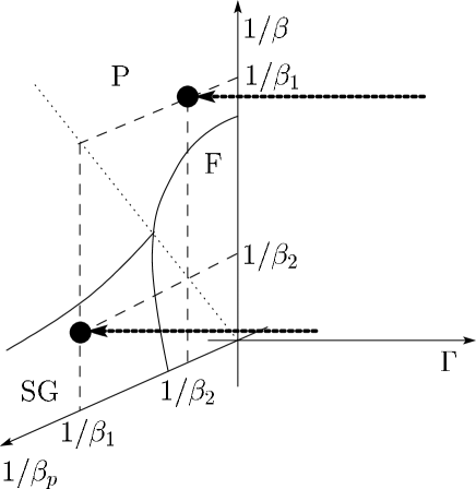
Setting $\beta_{2}=0$ in Eq. (160), (implying $p=1/2$, the symmetric distribution or the high-temperature limit), we find a simple equality on the performed work during NQA

$$\left[\langle\mathrm{e}^{-\beta_{1}W}\rangle_{\mathrm{QA}}\right]_{0}=\frac{(\cosh\beta_{1}J)^{N_{B}}}{(\cosh\beta_{1}\Gamma_{0})^{N}}.$$ (161)

The symmetric distribution ($\beta_{2}=0$ on the left-hand side) makes it possible to reduce the right-hand side to the above trivial expression. It is remarkable that NQA, which involves very complex dynamics, satisfies such a simple identity irrespective of the speed of annealing $T$. If we apply the Jensen inequality to the above equality, we can obtain the lower bound for the performed work as

$$\left[\langle W\rangle_{\mathrm{QA}}\right]_{0}\geq-\frac{N}{\beta}\log\left(\frac{(\cosh\beta J)^{\frac{N_{B}}{N}}}{\cosh\beta\Gamma_{0}}\right).$$ (162)

Here we generalize the inverse temperature to $\beta$ from the specific choice $\beta_{1}$. This lower bound is loose, since the direct application of the Jensen inequality to JE for NQA yields, after the configurational average with the symmetric distribution,

$$\left[\langle W\rangle_{\mathrm{QA}}\right]_{0}\geq\frac{1}{\beta}D(0|\beta)-\frac{N}{\beta}\log\left(\frac{(\cosh\beta J)^{\frac{N_{B}}{N}}}{\cosh\beta\Gamma_{0}}\right),$$ (163)

where $D(\beta|\beta^{\prime})$ is the Kullback-Leibler divergence defined as

$$D(\beta|\beta^{\prime})=\sum_{\{J_{ij}\}}\tilde{P}_{\beta}(\{J_{ij}\})\log\frac{\tilde{P}_{\beta^{\prime}}(\{J_{ij}\})}{\tilde{P}_{\beta}(\{J_{ij}\})}.$$ (164)

Here we defined the marginal distribution for the specific configuration $\{J_{ij}\}$ summed over all the possible gauge transformations,

$$\tilde{P}_{\beta}(\{J_{ij}\})=\frac{1}{2^{N}}\sum_{\{\xi_{i}\}}\prod_{\langle ij\rangle}P(J_{ij})=\frac{Z_{T}(\beta;\{J_{ij}\})}{2^{N}(2\cosh\beta J)^{N_{B}}}.$$ (165)

Since the Kullback-Leibler divergence does not become non-negative, the work performed by the transverse field during a nonequilibrium process in in the symmetric distribution (i.e. the left-hand side of Eq. (163)) does not exceed the second quantity on the right-hand side of Eq. (163). This fact means Eq. (162) was looser.

4.4.3 Exact relations involving inverse statistics

Beyond the above results, we can perform further non-trivial analyses for the nonequilibrium process in the special conditions. Let us next take the configurational average of the inverse of the Jarzynski equality, Eq. (153), as

$$\left[\frac{1}{\langle\mathrm{e}^{-\beta W}\rangle_{\mathrm{QA}}}\right]_{\beta_{p}}=\left[\frac{\left(2\cosh\beta\Gamma_{0}\right)^{N}}{Z_{T}(\beta;\{J_{ij}\})}\right]_{\beta_{p}}.$$ (166)

The application of the gauge transformation to the right-hand side yields

$$\left[\frac{1}{\langle\mathrm{e}^{-\beta W}\rangle_{\mathrm{QA}}}\right]_{\beta_{p}}=\sum_{\{J_{ij}\}}\frac{\exp\big{(}\beta_{p}\sum_{\langle ij\rangle}J_{ij}\xi_{i}\xi_{j}\big{)}}{(2\cosh\beta_{p}J)^{N_{B}}}\frac{\left(2\cosh\beta\Gamma_{0}\right)^{N}}{Z_{T}(\beta;\{J_{ij}\})}.$$ (167)

By summing the right-hand side over all the possible configurations of $\{\xi_{i}\}$ and dividing the result by $2^{N}$, we reach

$$\left[\frac{1}{\langle\mathrm{e}^{-\beta W}\rangle_{\mathrm{QA}}}\right]_{\beta_{p}}=\sum_{\{J_{ij}\}}\frac{Z_{T}(\beta_{p};\{J_{ij}\})}{2^{N}(2\cosh\beta_{p}J)^{N_{B}}}\frac{\left(2\cosh\beta\Gamma_{0}\right)^{N}}{Z_{T}(\beta;\{J_{ij}\})}.$$ (168)

If we set $\beta_{p}=\beta$ on the Nishimori line, this equation reduces to

$$\left[\frac{1}{\langle\mathrm{e}^{-\beta W}\rangle_{\mathrm{QA}}}\right]_{\beta}=\frac{(\cosh\beta\Gamma_{0})^{N}}{(\cosh\beta J)^{N_{B}}}.$$ (169)

Comparison of Eqs. (161) and (169) leads us to

$$\left[\langle\mathrm{e}^{-\beta W}\rangle_{\mathrm{QA}}\right]_{0}=\left(\left[\frac{1}{\langle\mathrm{e}^{-\beta W}\rangle_{\mathrm{QA}}}\right]_{\beta}\right)^{-1}.$$ (170)

As shown in Fig. 21, two completely different processes are nontrivially related by the resultant relation: One toward the Nishimori line and the other for the symmetric distribution.

Figure 21: Two different nonequilibrium processes in NQA through Eq. (170). We use the same symbols as in Fig. 12. The white circle denotes the target of the process on the right-hand side of Eq. (170), whereas the black dot is for the left-hand side.

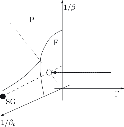
Let us further consider the inverse of Eq. (151) for the two-point correlation $O_{T}=\sigma^{z}_{i}\sigma^{z}_{j}$. We take the configurational average of both sides under the condition $\beta_{p}=\beta$ as

$$\left[\frac{1}{\langle\sigma^{z}_{i}\sigma^{z}_{j}\mathrm{e}^{-\beta W}\rangle_{\mathrm{QA}}}\right]_{\beta}=\frac{(\cosh\beta\Gamma_{0})^{N}}{(\cosh\beta J)^{N_{B}}}\left[\frac{1}{\langle\sigma^{z}_{i}\sigma^{z}_{j}\rangle_{\beta}}\right]_{\beta}.$$ (171)

The quantity on the right-hand side becomes unity by the gauge transformation as has been shown in the literatures [22, 7]. We thus obtain a simple exact relation

$$\left[\frac{1}{\langle\sigma^{z}_{i}\sigma^{z}_{j}\mathrm{e}^{-\beta W}\rangle_{\mathrm{QA}}}\right]_{\beta}=\frac{(\cosh\beta\Gamma_{0})^{N}}{(\cosh\beta J)^{N_{B}}},$$ (172)

which is another exact identity for processes of NQA.

The importance of the above equalities is still not clear. However it is true that we have little exact results on the nonequilibrium behavior of the spin glasses driven by quantum fluctuations as the transverse field. When we realize the quantum spin systems in experiments, the above results can play a roll as their indicators to verify their precisions and conditions. We should emphasize that the specialized tool to analyze spin glasses has facilitated the dynamical property in nonequilibrium process driven by quantum fluctuations. Beyond our analyses introduced here, we hope that more fascinating results on quantum computations would be obtained in the future with recourse to several techniques developed in statistical mechanics.

5 Summary

We looked over two topics lying between quantum information processing and statistical mechanics.

The first was the quantum error correction using the property of the topology. We prepare the redundant physical qubits in order to express the logical qubits we encode the specific information. Although we should deal with the quantum-many body systems, the used technique was proposed from the classical method in statistical mechanics. Statistical mechanics is available to facilitate to identify its precise location of the theoretical limitation to successfully infer the original state. In this direction with rich knowledge in statistical mechanics, we will be able to propose another ingenious way to give the quantum state more robustness and resilience as in the case of the depolarizing channel.

The second part was to improve the performance of quantum annealing away from the adiabatic-control case. The theoretical key was the Jarzynski equality. We suggest two ways to overcome the particular bottleneck in the adiabatic computation of quantum annealing. Both of the schemes would be needed for many-time repetition to produce the desired results. However we hope that the studies in this direction would give a novel technique beyond the ordinary limitations. The key point will be to enhance the possibility with the desired states. In the classical counterpart, recently several techniques are proposed with use of the population to reach the desired distribution, that is equilibrium state [49, 51, 50, 52]. Such a technique as in the classical case enables us to generate the particular quantum state with higher probability than expected by use of skillful techniques.

The bridge between the quantum information processing and statistical mechanics continues to lead us to frontiers, where we encounter novel and surprising results beyond expected ones from knowledge we obtain only from each side. We are at a position to look at the birth of such a fascinating interdisciplinary field. Don’t miss it.

References

- [1] A. Y. Kitaev, Ann. Phys. 303, 2 (2003).
- [2] E. Dennis, A. Kitaev, A. Landahl, and J. Preskill, J. Math. Phys. 43, 4452 (2002).
- [3] K. Binder and A. P. Young, Rev. Mod. Phys. 58, 801 (1986).
- [4] A. P. Young (ed.), Spin Glasses and Random Fields (World Scientific, Singapore, 1997).
- [5] N. Kawashima and H. Rieger, in Frustrated Spin Systems, ed. T. H. Diep (World Scientific, Singapore, 2004).
- [6] M. Mézard, G. Parisi and M. A. Virasoro, Spin Glass Theory and Beyond (World Scientific, Singapore, 1987).
- [7] H. Nishimori, Statistical Physics of Spin Glasses and Information Processing: An Introduction (Oxford Univ. Press, Oxford, 2001).
- [8] P. W, Shor, Phys. Rev. A 52, R2493 (1995).
- [9] A. B. Finnila, M. A. Gomez, C. Sebenik, S. Stenson and J. D. Doll, Chem. Phys. Lett. 219, 343 (1994).
- [10] T. Kadowaki and H. Nishimori, Phys. Rev. E 58, 5355 (1998).
- [11] T. Kadowaki, Study of optimization problems by quantum annealing, PhD thesis, Tokyo Institute of Technology, (1999); arXiv:0205020.
- [12] A. Das and B. K. Charkrabarti, Quantum Annealing and Related Optimization Methods, Lecture Notes in Physics Vol.679 Springer, Berlin, (2005).
- [13] G. E. Santoro and E. Tosatti, J. Phys. A 39, R393 (2006).
- [14] A. Das and B. K. Chakrabarti, Rev. Mod. Phys. 80, 1061 (2008).
- [15] S. Morita and H. Nishimori, J. Math. Phys. 49, 125210 (2008).
- [16] M. Ohzeki and H. Nishimori, J Comp. and Theor. Nanoscience 8, 963 (2011).
- [17] M. R. Garey and D. S. Johnson, Computers and Intractability: A Guide to the Theory of NP-Completeness, Freeman, San Francisco, (1979).
- [18] A. K. Hartmann and M. Weigt, Phase Transitions in Combinatorial Optimization Problems: Basics, Algorithms and Statistical Mechanics Wiley-VCH, Weinheim, (2005).
- [19] S. Kirkpatrick, S. D. Gelett and M. P. Vecchi, Science 220, 671 (1983).
- [20] E. Aarts and J. Korst, Simulated Annealing and Boltzmann Machines: A Stochastic Approach to Combinatorial Optimization and Neural Computing (Wiley, New York, 1984).
- [21] C. W. Gardiner, Handbook of Stochastic Methods (Springer, 1985 2nd Edition).
- [22] H. Nishimori, Prog. Theor. Phys. 66, 1169 (1981).
- [23] M. Ohzeki and H. Nishimori, J. Phys. A: Math. Theor. 42, 332001 (2009).
- [24] H. Nishimori and K. Nemoto, J. Phys. Soc. Jpn. 71, 1198 (2002).
- [25] J.-M. Maillard, K. Nemoto and H. Nishimori, J. Phys. A 36, 9799 (2003).
- [26] M. Ohzeki, H. Nishimori and A. N. Berker, Phys. Rev. E 77, 061116 (2008).
- [27] M. Ohzeki, Phys. Rev. E 79, 021129 (2009).
- [28] H. A. Kramers and G. H. Wannier, Phys. Rev. 60, 252 (1941).
- [29] F. Y. Wu and Y. K. Wang, J. Math. Phys. 17, 439 (1976).
- [30] H. Nishimori, J. Stat. Phys. 126, 977 (2007).
- [31] H. Bombin and M. A. Martin-Delgado, Phys. Rev. A 77, 042322 (2008).
- [32] H. G. Katzgraber, H. Bombin and M.-A. Martin-Delgado, Phys. Rev. Lett. 103, 090501 (2009).
- [33] M. Ohzeki, Phys. Rev. E 80, 011141 (2009).
- [34] T. M. Stace, S. D. Barrett and A. C. Doherty, Phys. Rev. Lett. 102, 200501 (2009).
- [35] T. M. Stace and S. D. Barrett, Phys. Rev. A 81, 022317 (2010).
- [36] M. Ohzeki, arXiv:1202.2593.
- [37] H. Bombin, R. S. Andrist, M. Ohzeki, H. G. Katzgraber and M. A. Martin-Delgado, to appear in Phys. Rev. X.
- [38] T. Jörg, F. Krzakala, J. Kurchan and A. C. Maggs, Phys. Rev. Lett. 101, 147204 (2008).
- [39] A. P. Young, S. Knysh and V. N. Smelyanskiy, Phys. Rev. Lett. 104, 020502 (2010).
- [40] R. D. Somma, C. D. Batista and G. Ortiz, Phys. Rev. Lett. 99, 030603 (2007).
- [41] M. Ohzeki, Phys. Rev. Lett. 105, 050401 (2010).
- [42] C. Jarzynski, Phys. Rev. Lett. 78, 2690 (1997).
- [43] C. Jarzynski, Phys. Rev. E 56, 5018 (1997).
- [44] P. Wocjan, C. F. Chiang, D. Nagaj and A. Abeyesinghe, Phys. Rev. A 80, 022340 (2009).
- [45] M. Ohzeki, H. Katsuda and H. Nishimori, J. Phys. Soc. Jpn. 80, 084002 (2011).
- [46] H. Tasaki, arXiv:0009244.
- [47] M. Campisi, P. Talkner and P. Hänggi, Phys. Rev. Lett. 102, 210401 (2009).
- [48] S. Morita, H. Nishimori and Y. Ozeki, J. Phys. Soc. Jpn. 75, 014001 (2006).
- [49] R. M. Neal, Statistics and Computing 11, 125 (2001).
- [50] Y. Iba, Trans. Jpn. Soc. Artif. Intel. 16, 279 (2001).
- [51] K. Hukushima and Y. Iba, AIP. Conf. Proc. 690, 200 (2003).
- [52] M. Ohzeki and H. Nishimori, J. Phys. Soc. Jpn. 79, 084003 (2010).