Evidence of Gunn-Peterson Damping Wings in High–$z$ Quasar Spectra: Strengthening the Case for Incomplete Reionization at $z\sim$6–7

Abstract

The spectra of several high–redshift ($z>6$) quasars have shown indications for a Gunn-Peterson (GP) damping wing, suggesting a substantial mean neutral hydrogen fraction ($\bar{x}_{\rm HI}^{\rm IGM}\mathrel{\hbox to0.0pt{\lower 4.0pt\hbox{\hskip 1.0pt$\sim$}\hss}\raise 1.0pt\hbox{$>$}}0.03$) in the $z\approx 6$ intergalactic medium (IGM). However, previous analyses assumed that the IGM was uniformly ionized outside of the quasar’s H ii region. Here we relax this assumption and model patchy reionization scenarios for a range of IGM and quasar parameters. Compared to uniform reionization, patchy reionization imprints a different average damping wing profile with an associated sightline-to-sightline scatter. We quantify the impact of these differences on the inferred $\bar{x}_{\rm HI}^{\rm IGM}$, by fitting the spectra of three quasars: SDSS J1148+5251 ($z=6.4189$), J1030+0524 ($z=6.308$), and J1623+3112 ($z=6.247$). We find that the best-fit values of $\bar{x}_{\rm HI}^{\rm IGM}$ in the patchy models agree well with the uniform case. More importantly, we confirm that the observed spectra favor the presence of a GP damping wing, with peak likelihoods decreasing by factors of $\mathrel{\hbox to0.0pt{\lower 4.0pt\hbox{\hskip 1.0pt$\sim$}\hss}\raise 1.0pt\hbox{$>$}}$ few – 10 when the spectra are modeled without a damping wing. We also find that the Ly$\alpha$ absorption spectra, by themselves, cannot distinguish the damping wing in a relatively neutral IGM from a damping wing in a highly ionized IGM, caused either by an isolated neutral patch, or by a damped Ly$\alpha$ absorber (DLA). However, neutral patches in a highly ionized universe ($\bar{x}_{\rm HI}^{\rm IGM}\mathrel{\hbox to0.0pt{\lower 4.0pt\hbox{\hskip 1.0pt$\sim$}\hss}\raise 1.0pt\hbox{$<$}}10^{-2}$), and DLAs with the large required column densities ($N_{\rm{\text{H\,\textsc{i}}}}\mathrel{\hbox to0.0pt{\lower 4.0pt\hbox{\hskip 1.0pt$\sim$}\hss}\raise 1.0pt\hbox{$>$}}{\rm{few}}\times 10^{20}{\rm{cm}^{-2}}$) are both rare. As a result, when we include reasonable prior probabilities for the line of sight (LOS) to intercept either a neutral patch or a DLA at the required distance of $\sim 40-60$ comoving Mpc away from the quasar, we find strong lower limits on the neutral fraction in the IGM, $\bar{x}_{\rm HI}^{\rm IGM}\mathrel{\hbox to0.0pt{\lower 4.0pt\hbox{\hskip 1.0pt$\sim$}\hss}\raise 1.0pt\hbox{$>$}}0.1$ (at 95% confidence). This supports earlier claims that a substantial global fraction of hydrogen in the $z\approx 6$ IGM is in neutral form.

1 Introduction

The epoch of reionization, when the radiation from early generations of astrophysical objects ionized the intergalactic medium (IGM), offers a wealth of information about cosmological structure formation and about physical processes in the early Universe. A variety of observations in the past few years have provided valuable insight into this epoch, through measurements of the cosmic microwave background (CMB) polarization anisotropies, quasar spectra, the kinetic Sunyaev-Zel’dovich (kSZ) signal and the evolution of the population of Ly$\alpha$ emitting galaxies. However, the interpretation of these observations remains controversial (e.g. Mesinger & Haiman 2004, 2007; Bolton & Haehnelt 2007a; Lidz et al. 2007a; Maselli, Ferrara & Gallerani 2009; Mesinger 2010; Mesinger & Furlanetto 2008; McQuinn et al. 2008; Dijkstra, Mesinger & Wyithe 2011; Dayal, Maselli & Ferrara 2011; Mesinger, McQuinn & Spergel 2011; Zahn et al. 2011a).

In particular, fully black Gunn-Peterson (GP) troughs (Gunn & Peterson, 1965), have been found in a number of $z>6$ Sloan Digital Sky Survey (SDSS) quasars, as well as in the quasar ULAS J1120+0641 recently discovered at $z=7.085$ (Mortlock et al., 2011) in the UKIDDS survey (Lawrence et al., 2007). The presence of these troughs suggests that these sources may be revealing the tail–end of reionization (see, e.g., the review by Fan, Carilli & Keating 2006). However, a neutral fraction as low as $\bar{x}_{\rm HI}^{\rm IGM}\sim 10^{-4}$ in a patch of the IGM is sufficient to produce a black GP trough – i.e. to make the flux undetectable at the wavelengths corresponding to resonant Ly$\alpha$ absorption. As a result, constraints inferred about global properties of reionization – such as the volume–averaged neutral hydrogen fraction $\bar{x}_{\rm HI}^{\rm IGM}$ – require modeling the spatial distribution and time–evolution of neutral hydrogen in the IGM (see e.g., Mesinger 2010).

A unique signature of significant neutral hydrogen in the IGM is the presence of a long tail of absorption, extending to wavelengths far away from the resonant GP trough – the so–called GP damping wing (Miralda-Escudé, 1998). The optical depth in the damping wing is $5-6$ orders of magnitude lower than in the resonant core of the Ly$\alpha$ line. Therefore this damping wing is detectable only if the neutral fraction is significant ($\bar{x}_{\rm HI}^{\rm IGM}\mathrel{\hbox to0.0pt{\lower 4.0pt\hbox{\hskip 1.0pt$\sim$}\hss}\raise 1.0pt\hbox{$>$}}$ few $\times 10^{-2}$).

In the SDSS quasars with a fully black GP trough, flux remains detectable over a wavelength range of a few $\times 10$ Å blueward of the Ly$\alpha$ line center, attributable to the nearly fully-ionized region surrounding the quasars. This region is highly ionized, but still contains sufficient residual H i to produce observable resonant line-of-sight (LOS) absorption, i.e. the Lyman $\alpha$ forest. Additionally, as the photons pass through the (possibly) neutral IGM in the foreground, the absorption in the GP damping wing causes a further depression of the flux. These two sources of Ly$\alpha$ absorption differ markedly: the resonant absorption within the ionized bubble strongly fluctuates with wavelength, whereas the absorption from the GP damping wing smoothly and monotonically increases blueward, with only a mild wavelength–dependence. This allows, in principle, the two different sources of opacity to be separated, given sufficiently high–quality quasar spectra (Cen & Haiman, 2000; Madau & Rees, 2000; Mesinger, Haiman & Cen, 2004). However, any robust interpretation requires modeling due to the near-degeneracy and uncertainty of the quasar and IGM properties (e.g., Mesinger & Haiman 2004, 2007; Bolton & Haehnelt 2007a, b; Mesinger & Furlanetto 2008; Maselli, Ferrara & Gallerani 2009).

In the case of the UKIDDS quasar ULAS J1120+0641, the GP trough is located at a wavelength much closer to the Ly$\alpha$ line center, i.e. the ionized region appears markedly smaller. As a result, the situation for this object is somewhat different from the SDSS quasars: the red GP damping wing can cause significant (10-20%) absorption on the red side of the Ly$\alpha$ line (Bolton et al., 2011). Therefore, the GP damping wing and the intrinsic quasar spectrum must be modeled simultaneously, and care must be taken to include the uncertainties in the latter (by comparison, the uncertainty in the intrinsic spectrum plays a sub-dominant role when deriving lower limits on the neutral fraction from the SDSS quasar spectra; Kramer & Haiman 2009). We defer the analysis of ULAS J1120+0641 to future work.

In our previous analysis of the SDSS quasars (Mesinger & Haiman 2007; hereafter MH07), we modeled the fluctuating resonant absorption within the ionized zone, detecting signatures of GP damping wing absorption in two out of three SDSS quasars: J1030+0524 and J1623+3112. Treating each as a free parameter, we were able to simultaneously place limits on the mean neutral fraction $\bar{x}_{\rm HI}^{\rm IGM}$, the quasars’ ionizing luminosities, and the sizes of the surrounding ionized regions. Most intriguingly, we statistically inferred the presence of a smooth absorption component corresponding to the GP damping wing, setting strong lower limits $\bar{x}_{\rm HI}^{\rm IGM}\mathrel{\hbox to0.0pt{\lower 4.0pt\hbox{\hskip 1.0pt$\sim$}\hss}\raise 1.0pt\hbox{$>$}}0.03$ for both J1030+0524 and J1623+3112 (with best–fit values of $\bar{x}_{\rm HI}^{\rm IGM}=1$ in both cases).

In MH07, a uniform ionizing background was assumed. However, the topology of reionization is likely very inhomogeneous, with ionized bubbles growing around highly clustered galaxies (e.g. Furlanetto, Zaldarriaga & Hernquist 2004; McQuinn et al. 2007; Trac & Cen 2007; Zahn et al. 2011b). The shape of the GP damping wing in a universe with such a “Swiss–cheese” reionization topology differs from that in a smoothly ionized IGM (as could result from more exotic reionization scenarios by X-ray photons; e.g. Haiman 2011).

Mesinger & Furlanetto (2008) compared GP damping wing profiles in these two different scenarios (see also McQuinn et al. 2008). Their results suggest that the difference could be significant, and that it can introduce a bias and scatter in neutral fraction constraints. In this paper, we use physical models for patchy reionization based on a semi-numerical simulation (Mesinger & Furlanetto, 2007), and infer constraints on the neutral fraction and on quasar parameters, using the observed spectra of the same three quasars that were previously analyzed in MH07. Our main goal is to assess whether allowing for patchy reionization significantly modifies previous results. Apart from relaxing the assumption of a uniform ionizing background, our analysis improves on MH07 by (i) using updated quasar redshift measurements and constraints on the quasars’ ionizing luminosities (Calverley et al., 2011), (ii) incorporating the fluctuating ionizing background from galaxies near the quasar, and (iii) a better statistical characterization of the confidence levels on the model parameters, explicitly contrasting results from a Bayesian analysis with a parametric bootstrapping procedure (as opposed to inferring probabilities from a Kolmogorov-Smirnov test as in MH07).

The rest of this paper is organized as follows. In § 2, we describe our analysis technique, including a description of the patchy reionization simulations, as well as a brief summary of how we generate mock absorption spectra and fit them to the observational data. In § 3, we present our results. In § 4, we discuss various aspects of our results, such as the origin of the constraints we obtain, and the robustness of our results, including the possible presence of damped Ly$\alpha$ systems (DLAs). In § 5, we summarize our key findings and present our conclusions. Throughout this paper, we adopt the background cosmological parameters ($\Omega_{\Lambda}$, $\Omega_{M}$, $\Omega_{b}$, $n$, $\sigma_{8}$, $H_{0}$) = (0.73, 0.27, 0.0455, 1, 0.76, 70 km s^-1 Mpc^-1), consistent with the seven–year results by the WMAP satellite (Komatsu, 2010). Unless stated otherwise, all quantities are quoted in comoving units.

2 Analysis

Our analysis has four distinct components: (i) running semi–numerical simulations to model patchy reionization, as well as the spatial distribution and mass function of halos, and the IGM density and velocity fields; (ii) using the simulations to create mock absorption spectra; (iii) modeling the quasars’ intrinsic emission spectrum; and (iv) comparing the observed and simulated absorption statistics. We first discuss our patchy reionization models (§ 2.1). Then in § 2.2 we present our procedure for creating mock Ly$\alpha$ absorption spectra (ii). Finally, we discuss the comparison of mock and observed spectra (iii-iv) in § 2.4.

2.1 Modeling Patchy Reionization

We use the publicly-available, semi-numerical code DexM (Mesinger & Furlanetto, 2007) to generate evolved density, halo, and ionization fields at $z=$ 6.5. Here we briefly outline the procedure, and refer the interested reader to Mesinger & Furlanetto (2007) for more details.

Our simulation box is $L=250$ Mpc on a side, with a particle grid cell size of 0.14 Mpc. Halos are filtered out of the 1800³ linear density field using excursion-set theory. Halo locations are then mapped to Eulerian coordinates at a given redshift using first-order Lagrangian perturbation theory (Zel’dovich, 1970). The resulting halo fields have been shown to match both the mass function and statistical clustering properties of halos in N-body simulations, well past the linear regime (Mesinger & Furlanetto, 2007).

The evolved (non-linear) density field is computed in the same manner, by perturbing the 1800³ Lagrangian density field. The resulting particle locations are then binned onto an Eulerian 600³ grid, and the corresponding evolved velocity field is re-computed from the density field. The final density and ionization fields thus have a grid cell size of 0.42 Mpc, approximately corresponding to the Jeans length in the ionized IGM at mean density. The statistical properties of the density and velocity fields have been shown to match those from a hydrodynamic simulation remarkably well (Mesinger, Furlanetto & Cen, 2011). Specifically, the agreement between the density fields at $z\approx 7$ is better than $\mathrel{\hbox to0.0pt{\lower 4.0pt\hbox{\hskip 1.0pt$\sim$}\hss}\raise 1.0pt\hbox{$<$}}$10% for both: (i) the PDF (smoothed on comparable scales) for roughly a dex around the mean (accounting for the vast majority of the volume), and (ii) the power spectra at $k\mathrel{\hbox to0.0pt{\lower 4.0pt\hbox{\hskip 1.0pt$\sim$}\hss}\raise 1.0pt\hbox{$<$}}$ few $\times$ Mpc^-1.

To generate the ionization field, we use the excursion-set formalism (Furlanetto, Zaldarriaga & Hernquist, 2004), which compares the number of ionizing photons produced in a region of a given scale to the number of neutral hydrogen atoms inside that region. Specifically, we identify ionized cells in our box as those which meet the criterion $f_{\rm{coll}}\geq\zeta^{-1}$, where $\zeta$ is an ionizing efficiency parameter and $f_{\rm{coll}}$ is the collapse fraction smoothed around a cell at $(\mathbf{x},z)$ on decreasing scales, $R$. The collapse fraction is computed using the resolved halo field, including halos down to a minimum mass of $1.7\times 10^{8}M_{\odot}$, corresponding to the atomic cooling threshold at $z\sim 6$. The resulting ionization morphologies match those generated with cosmological radiative transfer algorithms relatively well, with the power spectra agreeing to within $\sim$ 10–20% down to the Nyquist frequency (Zahn et al., 2011b).

We follow the procedure described in Mesinger & Dijkstra (2008) to model the galactic component of the ionization rate, $\Gamma_{\rm bg}$, inside the H ii regions, assuming that each galaxies ionizing luminosity is proportional to its halo mass. At every cell location ($\mathbf{x},z$), we sum the contributions of halos with mass $M_{i}$ at $\mathbf{x}_{i}$:

$$\Gamma_{\rm bg}(\mathbf{x},z)=\frac{(1+z)^{2}}{4\pi}\sigma_{H}\epsilon_{\rm{ion}}\sum_{i}\frac{M_{i}}{|{\bf x}-{\bf x_{i}}|^{2}}~{}e^{-|{\bf x}-{\bf x_{i}}|/\lambda}~{},$$ (1)

where $\sigma_{H}$ is the Lyman limit cross-section, and $\lambda$ is the ionizing photon mean free path inside HII regions. For simplicity and computational convenience, our fiducial analysis uses a constant mean free path, $\lambda=60$ (comoving) Mpc, consistent at 1-$\sigma$ with observations at $z\approx 6$ (Songaila & Cowie, 2010); we return to this point further below. The rate per unit mass at which ionizing photons are released into the IGM, $\epsilon_{\rm{ion}}$, governs the overall normalization of eq. (1). This normalization is chosen to match observations (see Calverley et al. 2011), resulting in an average ionization rate per hydrogen atom of $\bar{\Gamma}_{\rm bg}=10^{-13}~{}{\rm s^{-1}}$. In other words, we fix the mean galactic ionization rate to match Calverley et al. (2011), but use individual halo locations to model the local spatial fluctuations around this mean, according to eq. (1).

We vary the ionizing efficiency parameter, $\zeta$, to generate a suite of ionization fields corresponding to various values of $\bar{x}_{\rm HI}^{\rm IGM}$ at $z=6$. Specifically, we use the following eight different values: $\bar{x}_{\rm HI}^{\rm IGM}=\{0.01,0.06,0.10,0.38,0.53,0.64,0.73,0.88\}$. We then extract $2\times 10^{4}$ lines of sight (LOSs) centered on the two most massive halos in the simulation volume ($M\sim 3\times 10^{12}M_{\odot}$). The LOSs are drawn from randomly chosen directions. The resulting density, velocity and ionization LOSs are then used to construct mock Ly$\alpha$ spectra, as described below.

2.2 Modeling Quasar Absorption Spectra

We compute the residual, local neutral fraction along each LOS in the H ii region surrounding the quasar, whose extent we treat as a free parameter, $R_{S}$. Inside the ionized region, we assume ionization equilibrium with radiation from the quasar ($\Gamma_{\rm{Q}}$) and the background galaxies ($\Gamma_{\rm{bg}}$),

$$(\Gamma_{\rm{bg}}+\Gamma_{\rm{Q}})x_{\rm{\text{H\,\textsc{i}}}}n_{\rm{H}}=\alpha_{B}\chi_{\rm eff}n_{\rm{H}}^{2}(1-x_{\rm{\text{H\,\textsc{i}}}})^{2},$$ (2)

where $n_{\rm{H}}(\mathbf{x},z)$ is the local (non-linear) number density of hydrogen atoms, $x_{\rm{\text{H\,\textsc{i}}}}$ is the local neutral hydrogen fraction, $\chi_{\rm eff}=1.08$ accounts for additional electrons from singly-ionized Helium (assuming that the Helium and Hydrogen ionized fractions are equal with a Helium mass fraction of $Y_{\rm He}=0.24$), and $\alpha_{B}=1.7\times 10^{-13}\rm{cm}^{3}\rm{s}^{-1}$ is the case-B recombination coefficient. The latter is evaluated at the temperature $T=1.8\times 10^{4}$ K (consistent with recent measurements; Bolton et al. 2012).

Equation 2 is solved at every step along the LOS, using the non-linear density from our simulation. The contribution to the ionization rate from the quasar drops off approximately as the inverse square of the distance, and is given by

$$\Gamma_{Q}=\frac{1.6\times 10^{31}f_{\Gamma}}{4\pi d_{L}^{2}}\int_{\nu_{\rm{H}}}^{\infty}d\nu\left(\frac{\nu}{\nu_{\rm{H}}}\right)^{-1.8}\left(\frac{1+z}{1+z_{Q}}\right)^{0.8}\left(\frac{\sigma_{\nu}}{h\nu}\right)\rm{s}^{-1}.$$ (3)

Here $\sigma_{\nu}\approx 6.3\times 10^{-18}{\rm{cm}^{2}}(\nu/\nu_{\rm H})^{-3}$ is the frequency-dependent hydrogen ionization cross-section, $h$ is Planck’s constant, $z_{Q}$ is the observed redshift of the quasar, $z$ is the total redshift corresponding to a pixel along the LOS, including peculiar velocity [taking $(1+z)=(1+z_{0})(1+v_{pec}/c)$, where $z_{0}$ is the redshift that would correspond to the Hubble flow at the comoving distance of the pixel], $\nu_{\rm{H}}=3.29\times 10^{15}$Hz is the ionization threshold of hydrogen, $f_{\Gamma}$ is the quasar’s ionizing luminosity in units of $1.3\times 10^{57}\,\rm{s}^{-1}$ (following MH07), and $d_{L}=d_{L}(z_{0},z_{Q})$ is the luminosity distance between the quasar and the foreground pixel (see, e.g., Phillipps, Horleston & White 2002). Equation (3) further assumes an intrinsic $\nu^{-1.8}$ power-law spectrum for the ionizing radiation of the quasar, matching standard quasar templates (e.g. Telfer et al. 2002).

As in MH07, our model has three free parameters: (1) the LOS distance to the edge of the H ii region surrounding the quasar, $R_{S}$, (2) the quasar’s ionizing luminosity parametrized by $f_{\Gamma}$, and (3) the mean volume-weighted neutral fraction in the IGM, $\bar{x}_{\rm HI}^{\rm IGM}$. Our model grid covers a different range of $R_{S}$ for each quasar: in units of comoving Mpc, for J1148+5251, $R_{S}=\{37,39,41,43,45,47\}$, for J1030+0524, $R_{S}=\{52,54,56,58,60,62\}$, and for J1623+3112, $R_{S}=\{37,39,41,43,45,47\}$. In each case, we cover the range $f_{\Gamma}=\{0.1,0.4,0.7,1.0,1.3,1.6,1.9,4.0,6.0,8.0,10.0\}$, and the eight different values of $\bar{x}_{\rm HI}^{\rm IGM}$ listed above.

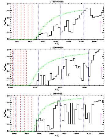
Figure 1: The continuum–normalized spectra of the three SDSS quasars used in this paper. The dotted (blue) vertical lines in each panel mark the boundaries of the three wide wavelengths bins used in the analysis, while the dashed (red) lines show the wavelengths corresponding to various assumed sizes ($R_{S}$) of the quasar’s ionized region explored in our models. The dot-dashed (green) curves indicate, for illustrative purposes only, the transmission attributed to the GP damping wing alone. These are the mean damping wings in the best-fit (without an R_S prior) models for each quasar, but our actual analysis includes the LOS-to-LOS scatter in both the damping wing and the resonant absorption). The magenta arrow on the right of each panel marks the location of the Ly$\alpha$ line at each quasar’s redshift.

It is worth pointing out that, in general, for a fixed neutral fraction, $R_{S}$ could be determined by the ionizing emissivity and the lifetime of the quasar, the surrounding galaxies, or a combination of both. As such, $R_{S}$ may be an integral, indirect measure of galaxy and quasar parameters (e.g., Wyithe & Loeb 2007), but here we simply take it to directly describe the ionization topology surrounding the quasar. We chose a range of $R_{S}$ values greater than or equal to the comoving distance between the redshift of the quasar and the redshift of the first (i.e. reddest) pixel in the quasar’s GP-trough. As we utilize the recently published revised redshift measurements of Calverley et al. 2011, our $R_{S}$ values are somewhat different (i.e., larger) than those in MH07. The wavelengths corresponding to our $R_{S}$ grid are indicated by the (red) vertical dashed lines in Figure 1.

For each given combination of $(R_{S},f_{\Gamma},\bar{x}_{\rm HI}^{\rm IGM})$, we create a mock absorption spectrum corresponding to each LOS extracted from our simulation box. The spectrum is simply assumed to be black at wavelengths corresponding to $R>R_{S}$ and is effectively ignored from our analysis. At $R<R_{S}$, the total optical depth includes resonant absorption from neutral HI inside the ionized region, as well as absorption through the damping wing by neutral hydrogen located outside $R>R_{S}$. We first create an array of observed wavelength bins $\lambda_{j}$, and for each bin, we sum the optical depth from every pixel $i$ along the LOS,

$$\tau_{j}={\sum_{i}}\frac{\sqrt{\pi}e^{2}f_{\alpha}}{m_{e}c}x_{i}n_{i}\frac{\delta s}{1+z_{0,i}}\phi_{\alpha}\left(\frac{\lambda_{j}}{1+z_{i}}\right),$$ (4)

where $e=4.8\times 10^{-10}$ esu is the charge of the electron, $f_{\alpha}=0.4162$ is the Ly$\alpha$ oscillator strength, $m_{e}=9.1\times 10^{-28}$ g is the mass of the electron, $z_{i}$ is the total redshift of pixel $i$, including its peculiar velocity, $x_{i}$ is the neutral fraction and $n_{i}$ is the total hydrogen density in pixel $i$, $\delta s/(1+z_{0,i})$ is the (physical, as opposed to comoving) width of the pixel, and $\phi_{\alpha}$ is the normalized absorption profile.

The frequency-dependence of the Ly$\alpha$ line is (Peebles, 1993, eq. 23.97)

$$\phi\left(\omega\right)=\frac{\Lambda_{\alpha}\left(\omega/\omega_{\alpha}\right)^{4}}{\left(\omega-\omega_{\alpha}\right)^{2}+\Lambda_{\alpha}^{2}\left(\omega/\omega_{\alpha}\right)^{6}/4},$$ (5)

where $\Lambda_{\alpha}=6.25\times 10^{8}{\rm s^{-1}}$ is the radiative decay rate. A common approach in the literature is to use the convolution of a Lorentzian (Peebles, 1993, eq. 23.43) with the thermal broadening, i.e. a Voigt profile (Press, Rybicki & Schneider, 1993) near the resonance $\omega\approx\omega_{\alpha}$ and an analytic solution for the damping wing far away from resonance that ignores Doppler broadening but includes the $\left(\omega/\omega_{\alpha}\right)^{4}$ Rayleigh-scattering tail (Miralda-Escudé, 1998). As our results may depend on intermediate regimes between the damping wing and line center, in principle, the thermally broadened line profile should be computed by convolving equation (5) with the temperature-dependent Doppler profile. In practice, we have approximated this full convolution with

$$\phi_{\alpha}\approx\phi_{\rm voigt}\left(\omega,T\right)\times\left(\omega/\omega_{\alpha}\right)^{4},$$ (6)

where $\phi_{\rm voigt}$ is the Voigt profile for our temperature $T$. This approximation approaches that given by Miralda-Escudé (1998) on the far red side of the damping wing.

In our patchy reionization models, specifying $\bar{x}_{\rm HI}^{\rm IGM}$ defines the ionization morphology. It is unlikely that the edge of the surrounding HII region will happen to lie at any given fixed distance, $R_{S}$. Therefore, in order to keep $R_{S}$ as an independent free parameter, we “shift” the ionization array (keeping the density array along the LOS fixed) by the minimal amount so that a neutral pixel falls at the location at $R_{S}$. However, in the highly-ionized models, we often encounter LOSs without any neutral pixels. In these cases, we keep the density and velocity field along the LOS, but we “recycle” the ionization array from another, randomly chosen LOS to make sure that a neutral pixel is located at $R_{S}$. This shifting is done in order to treat $R_{S}$ as a free parameter, while preserving the ionization morphology from the simulation at $R>R_{S}$ (which determines the GP damping wing). After presenting these conservative constraints, we then combine them with the (model-dependent) probability that a neutral pixel is, in fact, found at the radius $R_{S}$ (see the discussion in §3.2 below). This takes into account that a more ionized universe generally has larger HII regions by introducing a prior on $R_{S}$.

2.3 Model Parameters

In summary, our fiducial analysis has three free parameters (analogous to MH07):

• $\bar{x}_{\rm HI}^{\rm IGM}$ – the mean volume-weighted neutral fraction in the IGM. At a given redshift, $\bar{x}_{\rm HI}^{\rm IGM}$ is a function of $\zeta$ and $T_{\rm vir}$ (see below).
  

• $f_{\Gamma}$ – the quasar’s ionizing luminosity in units of $1.3\times 10^{57}\,\rm{s}^{-1}$.
  

• $R_{S}$ – the LOS distance to the edge of the H ii region surrounding the quasar.

Our models include additional parameters, which we either do not vary or which are used to derive the above quantities. Ideally one would like to explore as large a parameter space as possible; however, in practice, computational costs have limited us to vary at most three parameters simultaneously. In Sections 4.4–4.6 below, we perform additional investigations to assess the robustness of our results to degeneracies missing in our three–parameter models. The additional parameters include:

• $\zeta$ – the ionizing efficiency of high-redshift galaxies. This quantity can be defined as $\zeta=f_{\rm esc}f_{\ast}N_{\gamma}/(1+n_{\rm rec})$, where $f_{\rm esc}$ is the fraction of ionizing photons produced by stars that escape into the intergalactic medium (IGM), $f_{\ast}$ is the star formation efficiency, $N_{\gamma}$ is the number of ionizing photons per stellar baryon, and $n_{\rm rec}$ is the mean number of recombinations per baryon. For reference, $f_{\rm esc}=0.1$, $f_{\ast}=0.1$, $N_{\gamma}=4000$ (appropriate for PopII stars), and $n_{\rm rec}=1$ yield $\zeta=20$. As described above, we vary $\zeta$ to generate ionization maps, computing the resulting $\bar{x}_{\rm HI}^{\rm IGM}$.
  

• $T_{\rm vir}$ – the minimum virial temperature of halos hosting star-forming galaxies. As is common in reionization literature, we set this to the atomic-cooling threshold, $T_{\rm vir}=10^{4}$ K. Although $T_{\rm vir}$ could have a somewhat different value, the ionization morphology at fixed $\bar{x}_{\rm HI}^{\rm IGM}$ (the quantity of interest in this work) is fairly robust to (reasonable, physically-motivated) changes in $T_{\rm vir}$ (McQuinn et al., 2007; Mesinger, McQuinn & Spergel, 2011).
  

• $\bar{\Gamma}_{\rm bg}$ – the mean value of the galactic UVB. As mentioned above, we set this value to $\bar{\Gamma}_{\rm bg}=10^{-13}$ s^-1. Although this matches observations of the $z\sim 6$ Lyman alpha forest (e.g. Calverley et al. 2011), such measurements have large uncertainties. Luckily, our conclusions are not sensitive to the UVB, as we discuss below.
  

• $\lambda$ – the ionizing photon mean free path inside HII regions, generally set by Lyman limit systems (LLSs). We use a fiducial value of $\lambda=60$ (comoving) Mpc, consistent at 1-$\sigma$ with observations at $z\approx 6$ (Songaila & Cowie, 2010). The mean free path is used to compute the fluctuations in $\Gamma_{\rm bg}$, the galactic UVB. In principle, $\lambda$ is poorly constrained at high redshifts, and could even vary spatially (e.g. Crociani et al. 2011). However, our conclusions are not very sensitive to $\Gamma_{\rm{bg}}$, for several reasons. First, for most of the relevant spectral range and parameter choices, the quasar’s flux dominates the ionizing background, with galaxies becoming important only in the relatively unimportant high-$R_{S}$, low-$f_{\Gamma}$, low-$\bar{x}_{\rm HI}^{\rm IGM}$ regime (see more discussion of this point below in § 4.5, and also Lidz et al. 2007b and Bolton & Haehnelt 2007a). Second, the profile of $\Gamma_{\rm{bg}}$ (as a function of the distance from the quasar) is not degenerate with any of our three free parameters. Finally, as mentioned above, the average transmission is far more sensitive to the density field than to inhomogeneities in the background flux (Mesinger & Furlanetto, 2009a).

2.4 Fitting the free parameters in our model

2.4.1 Pixel Optical Depth Distributions

In order to compare our simulated spectra to the observations, we also need an intrinsic (unabsorbed) quasar emission template. These are obtained by fitting the Keck ESI observations of the quasars (e.g., White et al. 2003) only on the red side of the Ly$\alpha$ emission line, where IGM absorption is minimal. The intrinsic spectral fits are taken from MH07, to which we refer the interested reader for details. Briefly, the model fit to the data consists of the sum of a power-law continuum, a double-Gaussian Ly$\alpha$ emission line, and a N v emission line. The observed continuum-normalized flux in wavelength bin $j$ is then obtained as

$$\widetilde{F}_{obs,j}=F_{obs,j}{/{F_{cont,j}}}~{},$$ (7)

where $F_{cont,j}$ and $F_{obs,j}$, are the intrinsic and observed flux, respectively. We compare this observational signal with our mock continuum-normalized spectra, given by

$$\widetilde{F}_{sim,j}=\exp(-\tau_{j}).$$ (8)

Simulated optical depths can be far in excess of what is observable, so to ensure a fair comparison between simulation and observation, we impose a floor of minimum flux given by the observational errors ($\sigma_{obs,j}$, taken from White et al. 2003):

$$\widetilde{F}_{min,j}={A\sigma}_{obs,j}{/F}_{cont,j},$$ (9)

with the constant chosen to be $A=3$ for our analysis, corresponding to 3-$\sigma$ detections. For all values of $\widetilde{F}_{j}<\widetilde{F}_{min,j}$ we treat the simulated and observed continuum-normalized flux to be the same as zero flux. This floor corresponds to a maximum observable optical depth ranging between $\tau_{obs}=4.75$ to 5.5. The continuum-normalized spectra of the three quasars, subject to these conditions, are reproduced in Figure 1. Since present-day simulations do not have the dynamic range to model biases surrounding the bright, rare quasars, while at the same time resolving the Lyman-$\alpha$ forest, we excise the region 25 Å blue-ward of the Ly$\alpha$ peak from our analysis. This roughly corresponds to the expected mean radius ($\sim 10$ comoving Mpc) of the large–scale overdensity surrounding such quasars (e.g. Barkana & Loeb 2004).

We then compare the observed spectra to simulated mock spectra, using the two-sided Kolmogorov-Smirnov (KS) distance statistic $D_{KS}$ (Press et al., 1992), applied to the observed vs. simulated flux density PDFs. Each spectrum was binned into three wide wavelength ranges, with two of the bins chosen to lie red-ward of the pixels where the observed spectrum is consistent with zero flux – nominally corresponding to the apparent edge of the ionized bubble surrounding the quasar. The apparent edge falls within the third, bluest bin (see Figure 1). Within each of these three bins, the PDFs of the optical depth was obtained, for a given combination of $(R_{S},f_{\Gamma},\bar{x}_{\rm HI}^{\rm IGM})$, using all LOSs and all pixels within the bin. Each of the three model PDFs were then compared to the corresponding optical depth PDFs inferred from the observed spectra.

2.4.2 Best-Fit Models and Confidence Limits

In MH07, for each set of model parameters, the product of the three KS probabilities associated with the three $D_{KS}$ values, was used as the likelihood of that model. The probability $Q_{KS}(D_{KS})$ is given by the commonly used approximate analytic fitting formula (Press et al., 1992). However, this approach is potentially problematic, since: (i) the analytic formula is only accurate for “well-behaved” distributions; (ii) $\tau$ values in nearby pixels can be correlated, and (iii) the $\tau$ values in each of the $\sim$10 consecutive pixels within a bin are drawn from slightly different underlying probability distributions.

To address the impact of all of these issues, we explicitly compute the PDF of the KS distance statistic $D_{KS}$ in each of our models. We first compute the pixel optical depth PDF for the entire set of $2\times 10^{4}$ LOSs - this constitutes our best estimate for the $\tau$ PDF predicted in a given model. We then compare this prediction to the $\tau$ PDF for each individual LOSs in the same model, thus obtaining the (cumulative) PDF of $D_{KS}$ in this model. We have found that these CPDFs differ significantly from the fitting formula $Q_{KS}$ in Press et al. (1992). We traced these differences to the two reasons (i) and (ii) above. First, the floor imposed by equation (9) causes a pile-up of nearly identical optical depths (corresponding to the number of “black” pixels) in the $\tau$ PDF. This produces sharp steps in the sample CPDFs, and this unusual feature modifies the PDF of $D_{KS}$ (this effect is similar to a decrease in the number of effective data points). Second, correlations between neighboring pixels skew the CPDF away from $Q_{KS}$. We demonstrated this by first masking out the black pixels from the analysis, and then picking $\tau$ values from random LOSs to generate $2\times 10^{4}$ uncorrelated $\tau$ distributions. In this case, the CPDF of $D_{KS}$ indeed was consistent with $Q_{KS}(D_{KS})$.

For each $(R_{S},f_{\Gamma},\bar{x}_{\rm HI}^{\rm IGM})$ model (and in each of the three spectral bins $i$ of each quasar) we measure the KS distance $\bar{D}_{KS,obs}$, by comparing the $\tau$ CPDFs in the given model (averaged over all LOSs) with the corresponding $\tau$ CPDF in the quasar spectrum. We then construct the expected CPDF, $P_{(R_{S},f_{\Gamma},\bar{x}_{\rm HI}^{\rm IGM})}^{{\rm bin}~{}i}(>D_{KS})$, of the KS distance in this model, by comparing the $\tau$ CPDF of each LOS to the mean $\tau$ CPDF constructed from all LOSs. The probability that $D_{KS}$ exceeds $\bar{D}_{KS,obs}$, $P_{(R_{S},f_{\Gamma},\bar{x}_{\rm HI}^{\rm IGM})}^{{\rm bin}~{}i}(>\bar{D}_{KS,obs})$, is assigned to this model. Finally, multiplying the three probabilities in the three wavelength bins gives the model’s overall likelihood $p(R_{S},f_{\Gamma},\bar{x}_{\rm HI}^{\rm IGM})=\prod_{i=1}^{3}P_{(R_{S},f_{\Gamma},\bar{x}_{\rm HI}^{\rm IGM})}^{{\rm bin}~{}i}(>\bar{D}_{KS,obs})$ of the model. The best-fit model was identified as the one that maximizes this overall likelihood.

We next place confidence limits around this best-fit model by interpreting $p(R_{S},f_{\Gamma},\bar{x}_{\rm HI}^{\rm IGM})$ directly as Bayesian probability densities, and integrating these probability densities over our parameter space to obtain the confidence intervals. The results from this approach depend on the (arbitrary) parameterization of the parameter space volume. Here we chose $R_{S},\log f_{\Gamma}$ and $\log\bar{x}_{\rm HI}^{\rm IGM}$ – effectively adopting a uniform prior on these quantities. As a check on the robustness of these Bayesian confidence limits, we compare these results to those inferred from a parametric bootstrapping procedure (see § 4.2).

3 Results

3.1 Uniform Reionization

Before attempting to improve on the results in MH07, we first reproduced their main results, assuming, as in that paper, that the IGM outside $R_{S}$ is ionized by a spatially uniform background. A few of the details of our analysis, however, still differ from MH07:

(1) To accommodate the revisions in the redshifts of the three quasars (by up to $\Delta z\approx 0.03$; Carilli et al. 2010), we modify the boundaries of our three wavelength bins compared to those used by MH07. Likewise, we slightly adjust and expand the set of values for $R_{S}$ used in our grid of models. In particular, for J1030+0524, which has a Ly$\beta$ trough that lies at a significantly larger distance from the quasar than the Ly$\alpha$ trough, we impose a minimum size for the ionized region to $R>52$ Mpc, corresponding to the location of the Ly$\beta$ trough (as opposed to 40 Mpc in MH07, using the old redshift).

(2) Rather than having a uniform UVB inside the quasar’s HII region ($R<R_{S}$), we compute the inhomogeneous UVB from the nearby galaxies.

(3) We find the best-fit models using our own determination of the KS probabilities, rather than the standard fitting formula, as discussed in § 2.4.2 above.

(4) We add a strong prior for the probability distribution of the quasar’s ionizing flux $f_{\Gamma}$, based on the best–fit values and the errors obtained by Calverley et al. (2011). In practice, Calverley et al. (2011) quote errors on the logarithmic quasar luminosity $\ln L_{Q}$. For simplicity, we multiply the overall likelihood $p(R_{S},f_{\Gamma},\bar{x}_{\rm HI}^{\rm IGM})$, as defined in the previous section, by a Gaussian in $\ln f_{\Gamma}$, centered at $\ln f_{\Gamma}=(0.982,0.536,1.58)$ for J1030+0524, J1623+3112 and J1148+5251, respectively, and with the same uncertainty of $\sigma_{\ln f}=0.31$ for all three quasars.

(5) MH07 quoted the values of the parameters where the KS probabilities fell to $1/3$rd, $1/9$th, and $1/27$th of their peak values. For a 1D Gaussian, these would correspond to $\approx 1.5$, $\approx 2$, and $\approx 2.5\sigma$ confidence limits. The procedures discussed above allow us to integrate the likelihoods within the fixed contours, and to compute actual confidence limits in three dimensions. This is a particularly important change: due to the long non-Gaussian tails, and having a three-dimensional parameter space, we find that the confidence levels differ significantly from the simple 1D Gaussian expectation.

In Table 1, we show the parameter combinations where the likelihoods peak, as well as the best-fit models returned by the bootstrapping procedure. The first row for each quasar lists the results for the uniform-ionization case. For comparison, the values from MH07 are listed in the second row. The likelihoods peak at high neutral fractions for all three quasars, though none precisely at $\bar{x}_{\rm HI}^{\rm IGM}=1.0$. A notable difference from MH07 can be seen in the case of J1148+5251: the KS probability peaks at a higher neutral fraction ($\bar{x}_{\rm HI}^{\rm IGM}=0.88$ vs. 0.16), though this value is still consistent with the $1/3$rd probability contour of MH07. We also find significantly higher $R_{S}$ values for both J1030+0524 and J1623+3112 compared to MH07, caused by the increase in the intrinsic redshifts of these two quasars. This also leads to a factor of $\sim 2-3$ larger inferred quasar luminosities, which is not surprising: the material at the same observed wavelength is now farther from the quasar, so a larger intrinsic luminosity is needed to produce similar absorption.

When we use the same $Q_{KS}$ statistic as MH07, we further recover very similar lower limits on $\bar{x}_{\rm HI}^{\rm IGM}$, attributable to GP-damping wings for both J1030+0524 and J1623+3112. As in MH07, we also find that low values of $\bar{x}_{\rm HI}^{\rm IGM}$ can not be excluded for J1148+5251.

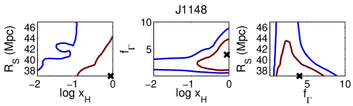
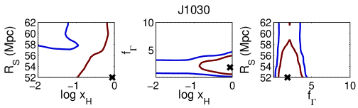
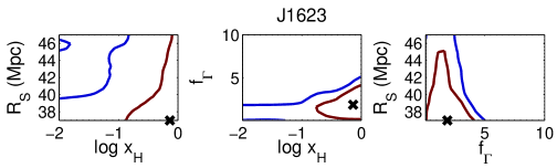
Figure 2: Confidence regions under the assumption that the IGM is ionized by a spatially uniform background. The three rows show the results for the three different quasars. In each row, the three different panels show the confidence contours in three different 2D planes, marginalized over the third parameter. The contours enclose 68 and 95% of the marginalized 2D likelihood. The location of the best-fit model is marked by an “x” in each panel.

We then switch to the new KS probability densities and integrate these over the parameters to obtain confidence levels. Our 68% and 95% two-dimensional confidence contours for each of the three quasars are shown in Figure 2. The constraints shown in each panel have been marginalized over the third parameter. Focusing on the further marginalized constraint on the single parameter $\bar{x}_{\rm HI}^{\rm IGM}$, we obtain a clear lower limit for J1148+5251 and J1623+3112 at about $\bar{x}_{\rm HI}^{\rm IGM}\mathrel{\hbox to0.0pt{\lower 4.0pt\hbox{\hskip 1.0pt$\sim$}\hss}\raise 1.0pt\hbox{$>$}}0.04$ while J1030+0524 has a somewhat stronger lower-limit at $\bar{x}_{\rm HI}^{\rm IGM}\mathrel{\hbox to0.0pt{\lower 4.0pt\hbox{\hskip 1.0pt$\sim$}\hss}\raise 1.0pt\hbox{$>$}}0.07$ .

3.2 Patchy Reionization

We next fit the spectra using our patchy reionization models. Unless stated otherwise, all constraints quoted below correspond to 95% confidence limits.

3.2.1 Results with a Uniform Prior on $R_{S}$

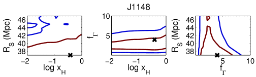
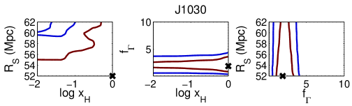
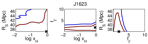
Figure 3: Confidence regions as in Figure 2, except in our patchy reionization models.

In Figure 3, we present the joint 2D 68% and 95% confidence contours for each quasar. As in the uniform reionization models, the best fits are located at high neutral fractions ($\bar{x}_{\rm HI}^{\rm IGM}\geq 0.38$). The most conspicuous change, however, is that the contours expand to significantly lower values of $\bar{x}_{\rm HI}^{\rm IGM}$, with the lowest value $\bar{x}_{\rm HI}^{\rm IGM}=0.01$ still falling inside the 95% CL on the $\bar{x}_{\rm HI}^{\rm IGM}-f_{\Gamma}$ plane. The single-parameter marginalized constraint yields essentially the same lower limit, weakened to $\bar{x}_{\rm HI}^{\rm IGM}\mathrel{\hbox to0.0pt{\lower 4.0pt\hbox{\hskip 1.0pt$\sim$}\hss}\raise 1.0pt\hbox{$>$}}0.02$ for all three quasars.

3.2.2 Adding a Physical $R_{S}$ Prior

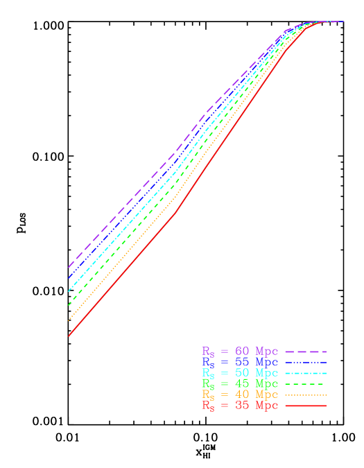
Figure 4: Fraction of the simulated lines-of-sight ($p_{\rm{LOS}}$) that intersect a neutral pixel within a given distance away from the quasar’s host halo, as labeled. These fractions are obtained from our patchy reionization models, and shown as a function of the global average neutral fraction $\bar{x}_{\rm HI}^{\rm IGM}$. The figure illustrates that intersecting a neutral patch within 35-60 (comoving) Mpc from the quasar is much less likely if the IGM is highly ionized.

As described in § 2.1, we shifted the ionization field in the patchy–reionization simulation, in order to ensure that the quasar’s ionization front can encounter a neutral pixel at the pre-specified location $R_{S}$. This was necessary to build up the statistics of the pixel optical depth PDF, and to be able to treat $R_{S}$ as one of our free parameters. However, as described above, these shifts make fits to the observed quasar spectra unfair: clearly, it is less likely to find a neutral pixel within a fixed radius $R_{S}$ in a highly ionized universe than in a more neutral universe. Thus, we next add in our analysis the prior probability for the LOS to intersect a neutral patch within $R_{S}$, taken from the patchy reionization simulations. These probabilities are shown in Figure  4.

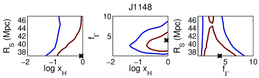
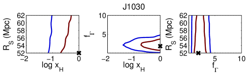
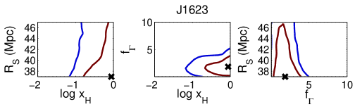
Figure 5: Confidence regions as in Figure 3, except priors were added for the probability of finding a neutral patch at $R_{S}$, taken from Figure 4.

In Figure 5 we present the confidence regions with these prior probabilities included. Unsurprisingly, adding the priors has the effect of excluding models with lower neutral fractions. For each of the three quasars, the 95% contour excludes models with $\bar{x}_{\rm HI}^{\rm IGM}\mathrel{\hbox to0.0pt{\lower 4.0pt\hbox{\hskip 1.0pt$\sim$}\hss}\raise 1.0pt\hbox{$<$}}0.05$. The single-parameter marginalized constraint yields $\sim 7$–9 times tighter limits, with J1148+5251 and J1623+3112 at $\bar{x}_{\rm HI}^{\rm IGM}\mathrel{\hbox to0.0pt{\lower 4.0pt\hbox{\hskip 1.0pt$\sim$}\hss}\raise 1.0pt\hbox{$>$}}0.14$ and J1030+0524at $\bar{x}_{\rm HI}^{\rm IGM}\mathrel{\hbox to0.0pt{\lower 4.0pt\hbox{\hskip 1.0pt$\sim$}\hss}\raise 1.0pt\hbox{$>$}}0.11$. We consider this to be the “fairest” statistic, and present these constraints as the main result of this work.

4 Discussion

4.1 The Detection of the GP Damping Wing

The main result of this paper is the strong lower limit on the mean neutral hydrogen fraction, $\bar{x}_{\rm HI}^{\rm IGM}\mathrel{\hbox to0.0pt{\lower 4.0pt\hbox{\hskip 1.0pt$\sim$}\hss}\raise 1.0pt\hbox{$>$}}0.1$. The mean GP damping wing absorption profiles, averaged over all LOSs in our best-fit models (in the patchy reionization case, with the $R_{S}$ prior included, and with the best-fits corresponding to the peak of the $P(D_{KS})$ likelihood) are shown, for illustrative purposes, by the dot-dashed (green) curves in Figure 1. We wish to confirm that our constraints arise from the statistical preference for these GP damping wings in the observed spectra, and not because of some other feature. To test this explicitly, we first re-fit the spectra, but this time ignoring the absorption by the GP damping wing. At the location of the best-fit model (i.e. with $R_{S}$ and $f_{\Gamma}$ fixed at the values listed in Table 1), the KS probabilities decrease by more than an order of magnitude for J1030+0524 and J1623+3112 and more than two orders of magnitude for J1148+5251. This demonstrates the sensitivity of the data to the presence/absence of the damping wings.

Even if the data is sensitive to the damping wings, however, our fits might not be sensitive to their presence, owing to degeneracies with other parameters. Indeed, we found that when we allow $R_{S}$ and $f_{\Gamma}$ to float, the best-fit value of $f_{\Gamma}$ was lower for J1623+3112 and J1148+5251 than in our fiducial models which include a damping wing. This is unsurprising – when the quasar flux is lower, the resonant opacity is increased and can compensate for the loss of the damping-wing absorption. However, in these damping-wing-less best-fit models, the peak probabilities are still factors of $\sim$6–11 below those in the original best-fit models. This demonstrates that our other parameters, e.g. a lower quasar ionizing flux, cannot fully mimic the presence of a GP damping wing.

4.2 Parametric Bootstrapped Confidence Contours and Scatter in the Damping Wing

The confidence contours shown in Figures 2,  3, and 5 rely on the assumption of an underlying flat prior on $\log\bar{x}_{\rm HI}^{\rm IGM}$ (as well as either a flat or a physical prior on $R_{S}$, and a Gaussian on $\log f_{\Gamma}$). Since the choice of the flat prior on $\log\bar{x}_{\rm HI}^{\rm IGM}$ is essentially arbitrary, we have replicated our entire analysis with an alternate, parametric bootstrapping procedure. Namely, we repeat the analysis discussed in § 2.4.2 another $2\times 10^{4}$ times, replacing the observed spectrum with the mock spectra generated along each of the $2\times 10^{4}$ LOSs in our best-fit model. This results in a set of $2\times 10^{4}$ new best–fit parameter combinations, which, in general, differ from the input values. The number of the new best-fit values in our 3D parameter space then directly yields the joint confidence levels. This method does not require an explicit prior on how the parameters are distributed, and is a common technique to estimate confidence levels (Press et al., 1992).

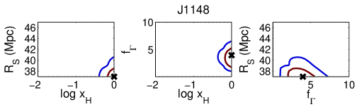
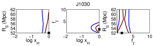
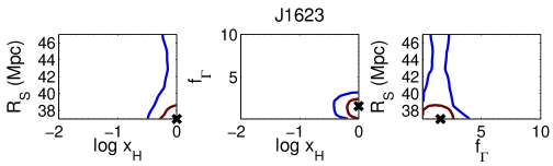
Figure 6: Confidence regions as in Figure 5, except that the parametric bootstrapping procedure, discussed in § 2.4.2, was used to estimate the confidence contours.

The results of this procedure are shown in Figure 6. The analysis includes the physical $R_{S}$ prior from Figure 4 (here used only to identify the initial best-fit models from which the LOSs are bootstrapped), and so this figure is to be compared to Figure 5. As this comparison reveals, the bootstrapping returns noticeably tighter contours. The single-parameter constraints on $\bar{x}_{\rm HI}^{\rm IGM}$ have tightened to $\bar{x}_{\rm HI}^{\rm IGM}\mathrel{\hbox to0.0pt{\lower 4.0pt\hbox{\hskip 1.0pt$\sim$}\hss}\raise 1.0pt\hbox{$>$}}0.48$ for J1030+0524 and $\bar{x}_{\rm HI}^{\rm IGM}\mathrel{\hbox to0.0pt{\lower 4.0pt\hbox{\hskip 1.0pt$\sim$}\hss}\raise 1.0pt\hbox{$>$}}0.62$ for J1623+3112 and J1148+5251. These constraints are weaker without the $R_{S}$ prior, in which case the lower limit for J1030+0524 is $\bar{x}_{\rm HI}^{\rm IGM}\mathrel{\hbox to0.0pt{\lower 4.0pt\hbox{\hskip 1.0pt$\sim$}\hss}\raise 1.0pt\hbox{$>$}}0.11$, J1623+3112 is $\bar{x}_{\rm HI}^{\rm IGM}\mathrel{\hbox to0.0pt{\lower 4.0pt\hbox{\hskip 1.0pt$\sim$}\hss}\raise 1.0pt\hbox{$>$}}0.07$, and J1148+5251 is $\bar{x}_{\rm HI}^{\rm IGM}\mathrel{\hbox to0.0pt{\lower 4.0pt\hbox{\hskip 1.0pt$\sim$}\hss}\raise 1.0pt\hbox{$>$}}0.14$. The lower limits derived for all three quasars in the corresponding Bayesian approaches are much weaker.

The large differences between the bootstrapped and the Bayesian confidence regions has a simple physical interpretation. The bootstrapping procedure samples the LOSs in our original best-fit models, and therefore the extent of the confidence regions reflect the LOS-to-LOS variations of the mock spectra in these best-fit models. For each quasar, this best-fit model corresponds to a nearly neutral IGM. Most importantly, in these nearly-neutral models, there is relatively little scatter in the strength of the damping wings – every LOS in each model contains a wide swath of neutral IGM. In contrast, low-$\bar{x}_{\rm HI}^{\rm IGM}$ models contain only relatively small and isolated neutral islands. For example, in the model with $\bar{x}_{\rm HI}^{\rm IGM}=0.01$, we find that neutral patches have a median diameter of only $\sim 7.5$ Mpc, and are typically separated by distances of order $\sim 100$ Mpc (see also Mesinger 2010). It is therefore very unlikely to find any LOS in our high-$\bar{x}_{\rm HI}^{\rm IGM}$ models, that is best fit by the narrow and weak damping wings in low-$\bar{x}_{\rm HI}^{\rm IGM}$ models. This results in the tight constraints generated by the bootstrapping procedure.

The situation is quite different when we estimate confidence levels directly from the Bayesian likelihoods. In this case, the probability density at each point in the parameter space is estimated using the LOS-to-LOS variations in that model, which generate the $\tau$ CPDFs. As a result, low-$\bar{x}_{\rm HI}^{\rm IGM}$ models are ruled out at a much weaker significance: these models have a large scatter. For example, in the model with $\bar{x}_{\rm HI}^{\rm IGM}=0.01$, we find that $\sim 5\%$ of the sightlines contain much larger neutral patches, with a diameter $\mathrel{\hbox to0.0pt{\lower 4.0pt\hbox{\hskip 1.0pt$\sim$}\hss}\raise 1.0pt\hbox{$>$}}35$ Mpc. We conclude, therefore, that the low-$\bar{x}_{\rm HI}^{\rm IGM}$ models have a relatively wide probability distribution of the KS-distance $D_{KS}$, and are therefore difficult to rule out at a high significance.

In principle, the scatter in resonant absorption may be important as well: the sightlines in the low-$\bar{x}_{\rm HI}^{\rm IGM}$ models that look more similar to the QSO (i.e. with $D_{KS}<\bar{D}_{KS,obs}$) might be those that have unusually high neutral density inside the HII region. To study this, we compare a sub-sample of “good-fit” LOSs in our $\bar{x}_{\rm HI}^{\rm IGM}=0.01$ model (i.e. LOSs having low values of $D_{KS}<\bar{D}_{KS,obs}$) to the full sample of $2\times 10^{4}$ sightlines. The low–$D_{KS}$ sub-sample has a noticeably stronger damping wing than the full sample. In contrast, the median resonant optical depths between the two samples are indistinguishable. We therefore confirm that the damping wing statistics are driving our conclusions and that the scatter in the damping wings make the Bayesian and the bootstrapping confidence limits different. These conclusions also show that the scatter in the damping wing strengths and shapes has a strong dependence on the average global ionization $\bar{x}_{\rm HI}^{\rm IGM}$, and imply that this can provide an additional probe of reionization (Mesinger & Furlanetto, 2008).

Apart from the three quasars analyzed here (as well as the $z=7.1$ source ULAS J1120+0641) with full GP troughs, currently there are $\sim 20$ quasars known at $z\mathrel{\hbox to0.0pt{\lower 4.0pt\hbox{\hskip 1.0pt$\sim$}\hss}\raise 1.0pt\hbox{$>$}}6$ (Willott et al., 2010b; Carilli et al., 2010). The sample is quite heterogeneous, and many quasars are too faint for useful spectroscopy. However, there are a handful of sources with spectra whose quality is similar to the quasars we analyzed, and yet they do not show a fully black GP trough. This may place an upper limit on $\bar{x}_{\rm HI}^{\rm IGM}$, since open sightlines, with no neutral patches, become rare in a nearly neutral universe.

4.3 Parameter Dependencies and Degeneracies

The confidence contours presented in Figures  2 and 3 illustrate a number of expected basic trends. Most importantly for our purposes, as the value of $\bar{x}_{\rm HI}^{\rm IGM}$ increases, the GP damping wing becomes stronger, and, in particular, dominates further blueward. In the patchy models, the dependence on $\bar{x}_{\rm HI}^{\rm IGM}$ arises from the width of the neutral slab(s) beyond $R>R_{S}$. This is different from the uniformly ionized models, in which the damping wing optical depth simply scales linearly with $\bar{x}_{\rm HI}^{\rm IGM}$, at every frequency. As $f_{\Gamma}$ increases, the resonant absorption inside $R<R_{S}$ is suppressed, and, as $R_{S}$ increases, the transmission window generally becomes larger. Degeneracies are therefore expected: a larger $R_{S}$ can be partly compensated by a stronger damping wing (larger $\bar{x}_{\rm HI}^{\rm IGM}$) and/or resonant absorption (a smaller $f_{\Gamma}$). Likewise, although their wavelength-dependence is different, in general, a weaker damping wing can be compensated, at least partly, by stronger resonant absorption. These trends are indeed visible in Figures 2 and 3 (although tempered by the priors on $f_{\Gamma}$ and on $R_{S}$).

4.4 Damped Lyman Alpha Systems

We have thus far considered GP absorption from neutral material in the IGM (i.e. at densities near the mean background density). Here we consider an alternative scenario, in which the IGM is highly ionized, and the apparently black GP trough in the quasar spectrum is caused instead by a single discrete absorber, i.e. a DLA, along the LOS.

We consider DLAs with the range of column densities of $N_{\rm{\text{H\,\textsc{i}}}}=\{10^{19},5\times 10^{19},10^{20},5\times 10^{20},10^{21},5\times 10^{21}\}\,\rm{cm}^{-2}$, placed at the same distances $R_{S}$ as we used for the edges of the surrounding HII regions in our fiducial analysis above. We create mock absorption spectra as outlined above, but replace the IGM damping wings from our reionization simulations with DLA damping wings. There are no neutral patches in this model, and the ionization field is taken to be the sum of the quasar’s ionizing flux, parameterized by $f_{\Gamma}$ as before, and the flux of the background galaxies, which is taken from the semi-numerical simulations as described above. Also as before, the flux is conservatively assumed to be zero beyond the DLA’s location ($R>R_{S}$). This assumes that the DLA casts a full shadow of the quasar along the LOS, and makes our constraints independent of the absorption statistics of the background IGM, away from the quasar.

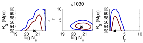
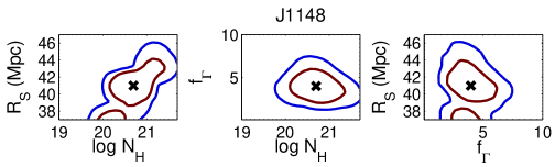
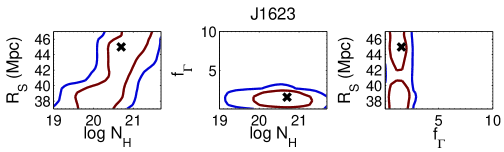
Figure 7: Confidence regions in the DLA models.

In Figure 7, we present joint two-dimensional confidence contours in this DLA model. As the figure shows, all three quasars require DLAs with very large column densities, with the same best-fit value of $N_{\rm{\text{H\,\textsc{i}}}}=5\times 10^{20}~{}{\rm cm^{2}}$. As Table 1 further shows, the bootstrapping procedure yields 68% CL lower limits on $N_{\rm{\text{H\,\textsc{i}}}}$ (marginalized over both $R_{S}$ and $f_{\Gamma}$) that range between $\approx 2\times 10^{19}-3\times 10^{20}~{}{\rm cm^{2}}$. Interestingly, Table 1 also shows that for J1030+0524, the lower limits on $N_{\rm{\text{H\,\textsc{i}}}}$ from the Bayesian and the bootstrapping analyses are similar, but for J1148+5251 and J1623+3112, the Bayesian limits are much weaker and closer to $N_{\rm{\text{H\,\textsc{i}}}}\sim 10^{19}~{}{\rm cm^{-2}}$. This is similar to the differences we found for the lower limits on $\bar{x}_{\rm HI}^{\rm IGM}$. However, unlike in the patchy reionization models, the DLA damping wings have, by definition, no scatter to account for this. To investigate the origin of this difference, we compared a sub-sample of “good-fit” LOSs — i.e. LOSs having low values of $D_{KS}<\bar{D}_{KS,obs}$ — in our low–$N_{\rm{\text{H\,\textsc{i}}}}$ model (with $N_{\rm{\text{H\,\textsc{i}}}}=10^{19}~{}{\rm cm^{-2}}$) to the full sample of $2\times 10^{4}$ sightlines. The low–$D_{KS}$ sub-sample had noticeably stronger resonant absorption than the full sample. We thus conclude that the difference between the Bayesian and bootstrapped lower limits for the DLA column densities is due to the scatter in the resonant absorption. This scatter is relatively more important in the low–$N_{\rm{\text{H\,\textsc{i}}}}$ models, and can produce LOSs that mimic stronger DLAs.

Most importantly, these results show that DLAs along the LOS can provide a plausible explanation of the spectra themselves. They could produce the black GP troughs, and, as shown in Table 1, the probabilities of the best-fit models are comparable to those in the models with incomplete reionization. However, finding DLAs with the high required column densities, relatively near the quasars, is improbable. Because of their rarity, the abundance of DLAs at high redshift is poorly known. Nevertheless, a modest extrapolation of existing DLA measurements between $4<z<6$ (Prochaska & Wolfe 2009; Songaila & Cowie 2010) to $z\approx 6.5$ imply the abundance $\sim 0.05$ DLAs with column densities $N_{\rm{\text{H\,\textsc{i}}}}\geq 2\times 10^{20}~{}{\rm cm^{2}}$ per unit redshift (see, e.g., Fig. 8 and Eq. 4 in Songaila & Cowie 2010). In our case, $\sim 50$Mpc corresponds to $\Delta z\sim 0.1$, implying that an abundance of $\sim 10$ DLAs per unit redshift is needed: this is more than two orders of magnitude higher than the above extrapolation suggests. In principle, the abundance of DLAs around quasars could be atypically high; however, at distances as far as 50 Mpc from the quasar, these biases should be negligible. Finally, the high-resolution spectra of these quasars show no evidence at the required distances of the low-ionization metal lines typical of DLAs (e.g. Ryan-Weber, Pettini & Madau 2006; Ryan-Weber et al. 2009; Simcoe 2006; G. Becker, private communication 2010).

4.5 The Impact of Ionizing Radiation from Galaxies

We turn now to the question of whether the ionizing radiation from the galaxies in the quasar’s ionized region is important for our conclusions. Generally, we expect that galaxies could be important for a combination of small $f_{\Gamma}$ (so that the quasar does not outshine the galaxies), small $\bar{x}_{\rm HI}^{\rm IGM}$ or $N_{\rm{\text{H\,\textsc{i}}}}$ (so that the damping wing absorption, which is independent of the galaxy background, does not dominate over the resonant absorption), and large $R_{S}$ (since the galaxy flux is only weakly dependent on $R$ within $R<R_{S}$, while the quasar flux drops as $\sim 1/R^{2}$)

To investigate the importance of galaxies more explicitly, we have re-run our analysis, with the ionizing radiation from the galaxies artificially turned off inside $R<R_{S}$. We find that for larger values of $f_{\Gamma}$ the galaxy flux can be ignored without much consequence. Furthermore, the presence of the galaxy flux has almost no effect on the best-fit locations or the peak likelihoods, with the impact restricted to the “periphery” of our parameter space, as expected above. In general, the contours tend to expand toward larger $R_{S}$ and smaller $\bar{x}_{\rm HI}^{\rm IGM}$ when the galaxy flux is not modeled.

As an example, we find that DLA models for J1623+3112 are most affected by the galaxy flux. The probability density at ($N_{\rm{\text{H\,\textsc{i}}}}=10^{19}\textrm{cm}^{-2}$, $R_{S}=47$ Mpc), integrated over $f_{\Gamma}$, is $\sim 3$ times higher when the galaxy contribution to the ionization radiation is neglected. The effect is reversed in (high–$N_{\rm{\text{H\,\textsc{i}}}}$, low–$R_{S}$) models where, for example, in the same quasar for $N_{\rm{\text{H\,\textsc{i}}}}=10^{20}\textrm{cm}^{-2}$ and $R_{S}=37$ Mpc, the probability density (again integrated over $f_{\Gamma}$) is $\sim 10$ times lower without galaxy fluxes. Nevertheless, the marginalized 1D constraints remain robust: without galaxies, following the format of Table 1, the constraints are $(f_{\Gamma},R_{S},\log N_{\rm{\text{H\,\textsc{i}}}})=(1.6^{+2.03}_{-0.53},39^{+8}_{-1.34},20.0^{+0.74}_{-0.61})$ with $\max\left(p\right)=0.21$.

4.6 The Impact of Self-Shielded Absorption Systems along the LOS

In this section, we consider the possibility that attenuation along the LOS is substantial, causing the QSO’s intensity to fall off more rapidly with distance than the approximate $\propto r^{-2}$ profile in equation (3). As mentioned above, a DLA or strong LLS along the sightline would be rare, and likely detectable in HIRES spectra. However, several lower column density systems aligning along the LOS could in principle strongly attenuate the flux, thereby mimicking a damping wing signature.

How degenerate are these two signatures? To answer this question, we perform an additional set of runs, repeating our fiducial analysis above, except without a damping wing, but instead attenuating the QSO flux by a factor of $\exp(-r/\lambda_{Q})$. We vary the effective LOS mean free path, $\lambda_{Q}$, from 60 Mpc down to 5 Mpc. We find that in all of these runs, the peak probabilities are reduced from our fiducial models with damping wings (Table 1). Specifically, for J1623+3112 / J1030+0524 / J1148+5251, the best-fit models have $\lambda_{G}=$ 50 / 40 / 15 Mpc, with $\max\left(p\right)$ lower than the peak probabilities in the fiducial, damping-wing-included results by 76 / 97 / 34 %.

To further explore the degeneracy between an altered (i.e. steeper) resonant absorption profile and our fiducial damping-wing absorption, we construct an unphysical, “worst-case” model. We again have no damping wings, but instead we adjust the flux, in each pixel, such that the average resonant optical depth precisely matches the total (resonant+damping) optical depth in our best-fit models from Table 1. We thereby allow an entirely arbitrary and contrived profile of the flux along the line-of-sight. (Indeed, in some cases, this profile is unphysical, as it rises with distance away from the quasar.) Even in this worst-case scenario, we find that the peak probabilities are still lower than in our fiducial cases, by 23% for J1148+5251, 11% for J1030+0524, and 22% for J1623+3112. This preference for the presence of a damping wing implies that the spectral fits are (mildly) sensitive to the smoothness of the damping wing profile (compared with the resonant absorption profile, which has significant pixel-to-pixel variations).

From both of the above tests, we conclude that even if there is unaccounted-for absorption of the QSO flux along the LOS, the observed spectra still prefer an IGM damping wing profile, at the tens of percents level.

5 Conclusions

The main result of this paper is the lower limit on the mean neutral hydrogen fraction, $\bar{x}_{\rm HI}^{\rm IGM}\mathrel{\hbox to0.0pt{\lower 4.0pt\hbox{\hskip 1.0pt$\sim$}\hss}\raise 1.0pt\hbox{$>$}}0.1$ (at 95% CL), inferred from the spectra of three $z>6$ quasars. Lower limits were previously obtained for the same three quasars by MH07, using simpler assumptions, and applying a less sophisticated statistical analysis. Our new results strengthen these previous limits. In particular, we have found that low neutral fractions are ruled out after relaxing the major assumption in MH07, of a uniform ionizing background. Unlike the lower limit obtained by MH07, which was driven by the pixel optical depth statistics in the spectral fitting alone, our new limit is driven by our additional modeling of the spatial distribution of neutral patches. We note that if we conservatively allow the size of the surrounding HII region to be a fully free parameter, independent of $\bar{x}_{\rm HI}^{\rm IGM}$, our constraints weaken to $\bar{x}_{\rm HI}^{\rm IGM}\mathrel{\hbox to0.0pt{\lower 4.0pt\hbox{\hskip 1.0pt$\sim$}\hss}\raise 1.0pt\hbox{$>$}}0.03$.

Our results arise through a statistical preference for a GP damping wing absorption component in the spectra. We confirm that peak likelihoods drop by a factor of several to more than an order of magnitude when the spectra are modeled without the damping wing component, implying the preference for significant neutral hydrogen in the IGM. Although such a damping wing could arise from a high-column density ($N_{\rm{\text{H\,\textsc{i}}}}\mathrel{\hbox to0.0pt{\lower 4.0pt\hbox{\hskip 1.0pt$\sim$}\hss}\raise 1.0pt\hbox{$>$}}{\rm{few}}\times 10^{20}{\rm{cm}^{-2}}$) DLA, such systems are very rare; furthermore, high-resolution spectra show no evidence, at the required distances, of the low-ionization metal lines typical of DLAs. In principle, the imprint of the damping wing could be mimicked by an alternate (not included in our fiducial model) evolution of the resonant absorption with distance from the quasar. We have shown, using a contrived worse-case toy-model, that the statistical preference for a damping wing can indeed decrease, but that it can not fully go away, even in this contrived model. Our analysis implies that reionization is not yet complete at $z\sim 6.2$.

Finally, we find different results when a Bayesian or a parametric bootstrapping method is used to estimate the confidence levels on our model parameters. We attribute this difference to the fact that the two methods are sensitive to the sightline-to-sightline scatter in the absorption statistics in the low– and the high–$\bar{x}_{\rm HI}^{\rm IGM}$ models, respectively. The scatter, in particular, in the GP damping wing strengths and shapes has a strong dependence on the average global ionization – as the global neutral fraction increases, the scatter is diminished. Our results demonstrate that this scatter could provide a useful additional diagnostic of the ionization topology of the IGM, when applied simultaneously to a larger quasar sample in the future.

6 Acknowledgments

We thank George Becker for discussing the presence of DLAs in HIRES spectra, and Xiaohui Fan for providing the ESI quasar spectra used in this paper. We would also like to thank David Spiegel for several informative discussions. ZH acknowledges support by the Polányi Program of the Hungarian National Office for Research and Technology (NKTH).

Model	$P(D_{KS})$ best-fit	$\max\left(p\right)$	Bootstrap best-fit	$\max\left(N_{bf}\right)$
	J1148+5251
uniform	$(4.0^{+2.35}_{-2.86},37^{+7.89}_{-0},0.88^{+0.12}_{-0.84})$	0.201	$(4.0^{+1.31}_{-2.34},37^{+1.05}_{-0},1.00^{+0}_{-0.38})$	7595
MH07	$(1.6,40,0.16)$	0.03	-	-
patchy	$(4.0^{+1.83}_{-2.86},37^{+7.37}_{-0},0.38^{+0.62}_{-0.36})$	0.248	$(4.0^{+1.83}_{-1.82},37^{+7.37}_{-0},0.64^{+0.36}_{-0.496})$	4691
$R_{S}$ prior	$(4.0^{+1.83}_{-2.86},37^{+9.47}_{-0},0.88^{+0.12}_{-0.73})$	0.196	$(4.0^{+1.31}_{-2.34},37^{+2.11}_{-0},1.00^{+0}_{-0.38})$	10126
DLA∗	$(4.0^{+2.35}_{-2.86},41^{+6}_{-4},20.7^{+0.72}_{-1.41})$	0.149	$(4.0^{+1.83}_{-1.82},41^{+2.84}_{-4},20.7^{+0.29}_{-0.28})$	8332
	J1030+0524
uniform	$(1.9^{+1.85}_{-0.76},52^{+10}_{-0},0.88^{+0.12}_{-0.81})$	0.194	$(1.6^{+1.63}_{-0.98},52^{+5.79}_{-0},1.00^{+0}_{-0.62})$	4293
MH07	$(1.0,41,1.0)$	0.34	-	-
patchy	$(1.9^{+1.85}_{-0.76},52^{+8.95}_{-0},1.00^{+0}_{-0.984})$	0.447	$(1.6^{+1.63}_{-0.98},52^{+8.42}_{-0},1.00^{+0}_{-0.89})$	3466
$R_{S}$ prior	$(1.9^{+1.85}_{-0.76},52^{+8.95}_{-0},1.00^{+0}_{-0.89})$	0.447	$(1.6^{+1.63}_{-0.98},52^{+10}_{-0},1.00^{+0}_{-0.52})$	3363
DLA∗	$(1.9^{+2.89}_{-0.76},54^{+6.95}_{-2},20.7^{+0.86}_{-1.27})$	0.259	$(1.9^{+1.85}_{-1.28},52^{+7.37}_{-0},20.7^{+0.57}_{-1.36})$	2563
	J1623+3112
uniform	$(1.9^{+1.85}_{-1.28},37^{+8.42}_{-0},0.73^{+0.27}_{-0.69})$	0.406	$(1.6^{+0.58}_{-1.5},37^{+2.11}_{-0},1.00^{+0}_{-0.82})$	1667
MH07	$(0.7,29,1.0)$	0.39	-	-
patchy	$(1.9^{+1.33}_{-1.8},37^{+8.95}_{-0},0.88^{+0.12}_{-0.86})$	0.472	$(1.3^{+0.88}_{-0.68},37^{+6.84}_{-0},1.00^{+0}_{-0.93})$	1565
$R_{S}$ prior	$(1.9^{+1.33}_{-1.28},37^{+8.95}_{-0},0.88^{+0.12}_{-0.74})$	0.464	$(1.6^{+0.58}_{-1.5},37^{+10}_{-0},1.00^{+0}_{-0.38})$	3290
DLA∗	$(1.9^{+1.85}_{-1.8},41^{+6}_{-4},21^{+0.42}_{-1.86})$	0.298	$(1.6^{+0.58}_{-1.5},45^{+2}_{-8},20.7^{+0.29}_{-0.56})$	1166

Table 1: The table shows the best-fit parameters in different models for the three quasar spectra (along with their 95% errors when appropriate, marginalized over the other two parameters in each case). For each quasar, the five rows describe the following models: (i) uniform reionization (§ 3.1), (ii) the earlier results of MH07, for reference, (iii) patchy reionization (§ 3.2.1), (iv) patchy reionization with a physical prior added for the distance $R_{S}$ to the nearest neutral patch (§ 3.2.2), and (v) a model in which the GP trough is caused by a DLA (§ 4.4). For each model, the four rows show (i) the best-fit parameters that maximize the probability based on the KS test (the values listed are for $(f_{\Gamma},R_{S}/\rm{Mpc},\bar{x}_{\rm HI}^{\rm IGM})$ in the reionization models, and $(f_{\Gamma},R_{S}/\rm{Mpc},\log N_{\rm{\text{H\,\textsc{i}}}}/\rm{cm}^{-2})$ in the DLA models), (ii) the value of this peak probability $p$; (iii) the best-fit parameters from the bootstrapping procedure (except MH07 did not perform any bootstrapping), and (iv) the peak number ($N_{bf}$) of bootstrap best–fits out of $2\times 10^{4}$ trials in this model. ^∗Note that we report 68% confidence intervals for $\log N_{\rm{\text{H\,\textsc{i}}}}$.

References

- Barkana (2002) Barkana R., 2002, New Astronomy, 7, 85
- Barkana & Loeb (2004) Barkana R., Loeb A., 2004, ApJ, 609, 474
- Bolton et al. (2012) Bolton J. S., Becker G. D., Raskutti S., Wyithe J. S. B., Haehnelt M. G., Sargent W. L. W., 2012, MNRAS, 419, 2880
- Bolton & Haehnelt (2007a) Bolton J. S., Haehnelt M. G., 2007a, MNRAS, 374, 493
- Bolton & Haehnelt (2007b) —, 2007b, MNRAS, 382, 325
- Bolton et al. (2011) Bolton J. S., Haehnelt M. G., Warren S. J., Hewett P. C., Mortlock D. J., Venemans B. P., McMahon R. G., Simpson C., 2011, MNRAS, 416, L70
- Calverley et al. (2011) Calverley A. P., Becker G. D., Haehnelt M. G., Bolton J. S., 2011, MNRAS, 412, 2543
- Carilli et al. (2010) Carilli C. L. et al., 2010, ApJ, 714, 834
- Cen & Haiman (2000) Cen R., Haiman Z., 2000, ApJL, 542, L75
- Crociani et al. (2011) Crociani D., Mesinger A., Moscardini L., Furlanetto S., 2011, MNRAS, 411, 289
- Croft (1998) Croft R. A. C., 1998, in Eighteenth Texas Symposium on Relativistic Astrophysics, A. V. Olinto, J. A. Frieman, & D. N. Schramm, ed., pp. 664–+
- Dayal, Maselli & Ferrara (2011) Dayal P., Maselli A., Ferrara A., 2011, MNRAS, 410, 830
- Dijkstra, Mesinger & Wyithe (2011) Dijkstra M., Mesinger A., Wyithe J. S. B., 2011, MNRAS, 414, 2139
- Fan, Carilli & Keating (2006) Fan X., Carilli C. L., Keating B., 2006, ARA&A, 44, 415
- Furlanetto, Zaldarriaga & Hernquist (2004) Furlanetto S. R., Zaldarriaga M., Hernquist L., 2004, ApJ, 613, 1
- Gallerani, Choudhury & Ferrara (2006) Gallerani S., Choudhury T. R., Ferrara A., 2006, MNRAS, 370, 1401
- Gunn & Peterson (1965) Gunn J. E., Peterson B. A., 1965, ApJ, 142, 1633
- Haiman (2011) Haiman Z., 2011, Nature, 472, 47
- Komatsu (2010) Komatsu E. e. a., 2010, ApJ, submitted, e-print arXiv:1001.4538
- Kramer & Haiman (2009) Kramer R. H., Haiman Z., 2009, MNRAS, 400, 1493
- Lawrence et al. (2007) Lawrence A. et al., 2007, MNRAS, 379, 1599
- Lidz et al. (2007a) Lidz A., McQuinn M., Zaldarriaga M., Hernquist L., Dutta S., 2007a, ApJ, 670, 39
- Lidz et al. (2007b) —, 2007b, ApJ, 670, 39
- Madau & Rees (2000) Madau P., Rees M. J., 2000, ApJL, 542, L69
- Maselli, Ferrara & Gallerani (2009) Maselli A., Ferrara A., Gallerani S., 2009, MNRAS, 395, 1925
- McQuinn et al. (2007) McQuinn M., Lidz A., Zahn O., Dutta S., Hernquist L., Zaldarriaga M., 2007, MNRAS, 377, 1043
- McQuinn et al. (2008) McQuinn M., Lidz A., Zaldarriaga M., Hernquist L., Dutta S., 2008, MNRAS, 388, 1101
- Mesinger (2010) Mesinger A., 2010, MNRAS, 407, 1328
- Mesinger & Dijkstra (2008) Mesinger A., Dijkstra M., 2008, MNRAS, 390, 1071