A Tentative Gamma-Ray Line
from Dark Matter Annihilation
at the
Fermi Large Area Telescope
Abstract
The observation of a gamma-ray line in the cosmic-ray fluxes would be a smoking-gun signature for dark matter annihilation or decay in the Universe. We present an improved search for such signatures in the data of the Fermi Large Area Telescope (LAT), concentrating on energies between and . Besides updating to 43 months of data, we use a new data-driven technique to select optimized target regions depending on the profile of the Galactic dark matter halo. In regions close to the Galactic center, we find a indication for a gamma-ray line at . When taking into account the look-elsewhere effect the significance of the observed excess is . If interpreted in terms of dark matter particles annihilating into a photon pair, the observations imply a dark matter mass of and a partial annihilation cross-section of when using the Einasto dark matter profile. The evidence for the signal is based on about photons; it will take a few years of additional data to clarify its existence.
2(10.1,0) MPP-2012-73
1 Introduction
The existence of dark matter (DM) in the Universe is a by now well established fact, supported by numerous of observations that range from the time of matter/radiation equality until today [Komatsu:2010fb]. A plethora of possible particle physics scenarios for DM exists, among which the currently leading hypothesis are weakly interacting massive particles (WIMPs) that are thermally produced in the early Universe [Jungman:1995df, Bertone:2004pz, Bergstrom:2009ib]. WIMPs could be produced at particle colliders like the CERN LHC, they could be observed via WIMP-nucleon scattering in low-background experiments, and, due to their self-annihilation in the Universe, they could contribute to the cosmic-ray fluxes (see Ref. [Cirelli:2012tf] for a recent review).
Among the different particle species produced in WIMP annihilation, gamma rays are of particular importance, as they propagate essentially unperturbed and preserve spatial information about their sources. This information is exploited for efficient signal/background discrimination in searches for gamma-ray signatures from e.g. dwarf galaxies [Essig:2009jx, Scott:2009jn, Abramowski:2010aa, Aleksic:2011jx, Abdo:2010ex, Ackermann:2011wa, GeringerSameth:2011iw, Cholis:2012am, Mazziotta:2012ux] or the Galactic center (GC) [Aharonian:2006wh, Hooper:2011ti, Vitale:2011zz, Abramowski:2011hc].
Besides spatial signatures, signatures in the energy spectrum of the gamma-ray flux play a major role in DM searches. It was noted long ago [Bergstrom:1988fp] that the two-body annihilation of DM into photons produces monochromatic gamma rays that could stand out of the otherwise continuous astrophysical fluxes as a clear smoking gun signature [Rudaz:1989ij, Bergstrom:1997fh, Ullio:1997ke, Bern:1997ng, Bergstrom:2004nr, Bertone:2009cb, Bertone:2010fn]. In most cases, the line signal is expected to be extremely faint, as its production is one-loop suppressed. However, it can be enhanced in many scenarios, like non-minimal variations of the MSSM [Profumo:2008yg, Ferrer:2006hy], singlet DM [Profumo:2010kp], hidden U(1) DM [Dudas:2009uq, Mambrini:2009ad], effective DM scenarios [Goodman:2010qn], scenarios with strong annihilation into the higgs boson and a photon [Jackson:2009kg] or inert higgs doublet DM [Gustafsson:2007pc]; these gamma-ray lines would be indeed in reach of current technology [Bringmann:2011ye]. Additional prominent spectral features in the gamma-ray flux are generated by the emission of internal bremsstrahlung (IB) photons during DM annihilation [Beacom:2004pe, Bergstrom:2004cy, Birkedal:2005ep, Bergstrom:2005ss, Bringmann:2007nk].
Since more than three years, the Fermi Large Area Telescope (LAT), which is the main instrument on the Fermi Gamma-ray Space Telescope [Atwood:2009ez], measures the gamma-ray sky with an unprecedented precision, searching—amongst others—for DM signals [Baltz:2008wd]. Previous searches for spectral signatures from DM annihilation [Abdo:2010nc, Vertongen:2011mu, Fermi:Symp2011Talk, Edmonds:2011PhD, Feng:2011ab] were exclusively concentrating on gamma-ray lines (an earlier analysis using EGRET data can be found in Ref. [Pullen:2006sy]). A first dedicated search for IB signatures was recently presented in Ref. [Bringmann:2012vr]; in this paper, a week indication for a spectral signature close to the GC was reported.
The purpose of the present work is to update and refine the existing searches for gamma-ray lines from DM annihilation in Fermi LAT data. In particular, we are interested in a further investigation of the signature reported in Ref. [Bringmann:2012vr]. Besides taking into account all data collected so far (43 months), and making use of the most up-to-date publicly available event selections, we employ a new data-driven algorithm to find target regions that maximize the signal-to-noise ratio (SNR) for different profiles of the Galactic DM halo. Since we are looking for very faint signatures, this is extremely important. An inefficient choice of the target region can easily hide a DM signal. We concentrate on line energies between and and use the data below for target region selection.
The rest of this paper is organized as follows: In Section 2, we explain in detail the DM signal we are looking for, the treatment of the Fermi LAT data, the target region selection and the spectral analysis; in Section 3 we present our main results; a discussion of instrumental systematics, further tests and comparison with previous work can be found in Section 4; we conclude in Section 5. Event tables are provided in Appendix A.
2 Data Analysis
2.1 DM annihilation in the Galactic halo
The gamma-ray flux from DM particles annihilating into a photon pair inside the Galactic DM halo is (for a Majorana WIMP) given by
| (2.1) |
where is the angle to the GC. Here, is the DM mass, the partial annihilation cross-section for , the gamma-ray line energy and the DM distribution as function of the Galactocentric distance . The coordinate runs along the line-of-sight, and , where denotes the distance between Sun and GC.
We consider five reference DM profiles, all normalized to at position of the Sun [Catena:2009mf, Salucci:2010qr]: (1) The Einasto profile, favored by the latest -body simulations [Navarro:2003ew, Springel:2008cc, Pieri:2009je],
| (2.2) |
with and . (2) The commonly used cored isothermal profile
| (2.3) |
with (see e.g. Ref. [Salucci:2007tm] for observational arguments in favor of cored DM profiles). (3-5) The generalized Navarro-Frenk-White (NFW) profile
| (2.4) |
with . Here, parametrizes the profile’s inner slope, and reproduces the usual NFW profile [Navarro:1996gj, Abdo:2010nc]. The presence of the super-massive black hole [Gondolo:1999ef] or adiabatic contraction [Blumenthal:1985qy, Gnedin:2003rj, Gustafsson:2006gr, Gnedin:2011uj] can steepen the inner profile, which is here effectively taken into account by allowing that . To this end, we consider the three reference values , which are compatible with microlensing and dynamical observations [Iocco:2011jz]. Note that changing the slope of the inner profile in principle also affects the profile normalization. Since we are here mainly interested in the shape of the DM signal, however, we will keep fixed for simplicity.
2.2 Data selection
In the present analysis, we take into account 43 months of data (from 4 Aug 2008 to 8 Mar 2012) with energies between 1 and 300 GeV.111High level data of the LAT is available at http://fermi.gsfc.nasa.gov. We apply the zenith-angle cut in order to avoid contamination with the earth albedo, as well as the recommended quality-filter cut DATA_QUAL==1. For comparison and cross-checks, we make use of both the SOURCE and ULTRACLEAN events selections (both Pass 7 Version 6). The former features an effective area that is relatively larger by about at 100 GeV, the latter a lower contamination with residual charged cosmic rays (CRs). In the main analysis, front- and back-converted events are considered simultaneously, in order to minimize statistical errors. The selection of events as well as the calculation of exposure maps is performed using the 6 Oct 2011 version of ScienceTools v9r23p1.222See http://fermi.gsfc.nasa.gov/ssc/data/analysis for the standard chains. For everything else we use our own software.
2.3 Target regions & observed fluxes
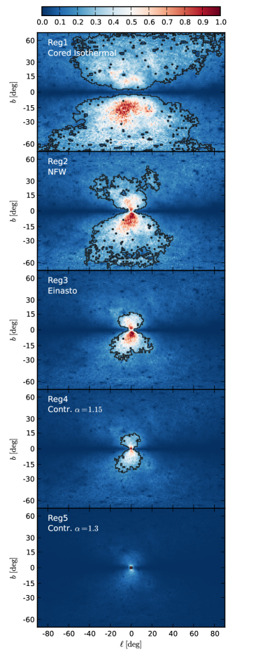
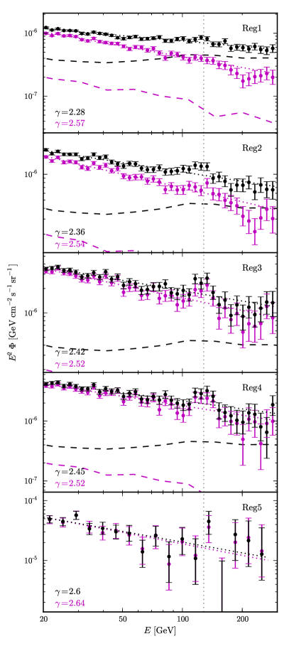
Right panel: From top to bottom, the panels show the – gamma-ray (+ residual CR) spectra as observed in Reg1 to Reg5 with statistical error bars. The SOURCE and ULTRACLEAN events are shown in black and magenta, respectively. Dotted lines show power-laws with the indicated slopes; dashed lines show the EGBG + residual CRs. The vertical gray line indicates .
The optimal target region for gamma-ray line searches maximizes the SNR and depends on both, the morphology of the DM signal and the morphology of the background flux. For a particular Galactic DM profile, the former is given by Eq. (2.1); the latter has to be in principle determined from a modeling of gamma-ray diffuse and point sources at – energies. The basic strategy that we follow here is to approximate the background morphology above 20 GeV by the spatial distribution of gamma rays measured between and .
From events in the energy range –, we produce a two-dimensional count map that covers an area of Galactic latitude and Galactic longitude, using a cylindrical equal-area projection with one square-degree pixel size.333Because of this projection we exclude data with . This does not affect the results. Note that we use the convention throughout. For each pixel , we derive the number of expected signal events from Eq. (2.1), whereas the number of actually measured events is denoted by . We need only up to an overall normalization, since we leave and unspecified at this point. As long as the signal is only a weak perturbation, the SNR in each pixel can be estimated by . Note that throughout the entire analysis, the angular resolution of the LAT— for to energies [Fermi:performancePASS7]—is neglected.
We define the optimal target region as the set of pixels for which the integrated SNR
| (2.5) |
is maximized. To find , we use the approximate but efficient algorithm from Ref. [Bringmann:2012vr]. The resulting target regions, optimized for our five reference DM profiles, are shown in the left panels of Fig. 1 by the black lines. The colors indicate the signal-to-background ratio , with an arbitrary but common normalization. In case of a cored isothermal profile (Reg1), the target region is largest and reaches up to latitudes of . The smallest region (Reg5) corresponds to a compressed profile with inner slope , and contains the central degree of the GC only. In most cases, the regions are more extended south from the GC. This is a consequence of a slight north/south asymmetry in the observed diffuse gamma-ray flux (see e.g. Ref. [FermiLAT:2012aa]). Note that the regions are only optimal as long as signal contributions are small. In the presence of a potential signal these regions can be further optimized, which we leave for future work.
We extract from the LAT data the gamma-ray flux measured in each of the five target regions. The corresponding energy spectra between and are shown in the right panels of Fig. 1 for both, SOURCE (black) and ULTRACLEAN (magenta) event classes. The residual CR contamination of the SOURCE event selection is best visible in Reg1 as a sizeable difference between the SOURCE and ULTRACLEAN fluxes. This is further illustrated by the dashed lines, which show the expected flux of residual CRs plus the extragalactic gamma-ray background (EGBG) for comparison [Fermi:BackgroundModels]. Remarkably, in Reg3 and Reg4 a pronounced bump at energies around (indicated by the vertical dotted line) can be easily recognized by eye; this spectral feature will turn out to be the best candidate for a gamma-ray line in the Fermi LAT data between and .
2.4 Spectral analysis
In order to search for gamma-ray lines in Reg1 to Reg5, we perform a shape analysis of the energy spectra shown in Fig. 1 (though with much smaller energy bins). For a given gamma-ray line energy , this analysis is done in a small energy window that contains . The exact positions of the energy windows adopted during the main analysis are shown in Fig. 2. Since the energy windows follow the gamma-ray line energy, this method is known as “sliding energy window” technique [Pullen:2006sy, Abdo:2010nc, Vertongen:2011mu, Bringmann:2011ye, Bringmann:2012vr].
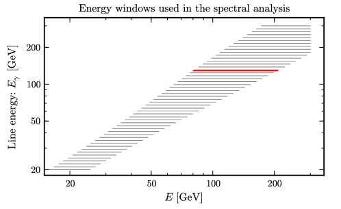
We can conveniently parametrize the boundaries of the energy window as
| (2.6) |
The sizes of the adopted energy windows vary between at low energies, which is a few times wider than the LAT energy resolution, and at high energies, in order to compensate for the lower number of events. The choice of the energy window size is somewhat arbitrary, but depends in principle on the uncertainties in the background curvature, the effective area and on the available statistics. We will discuss below how a change of the window size affects the results.
Within the adopted energy windows, we fit the spectra from Fig. 1 with a simple three-parameter model,
| (2.7) |
Background fluxes are here approximated by a single power law with a free spectral index and normalization , whereas the monochromatic DM signal has a free normalization while its position remains fixed during the fit. Note that, after fixing the experimental conditions and the profile of the Galactic DM halo, the annihilation cross-section is related to by a straightforward rescaling.
The best-fit model parameters are obtained by maximizing the likelihood function , where is the Poisson probability distribution function; here, () denotes the number of measured (expected) events in energy bin . In general, is a function of the model parameters and calculated by multiplying the above three-parameter model with the exposure of the target region, and convolving the resulting function with the effective energy dispersion of the LAT. The details of this calculation are discussed below in section 2.5. In our analysis we use energy bins that are much smaller than the energy resolution of the LAT, such that the analysis becomes independent of the actual binning and hence effectively “unbinned”.444We use 300 logarithmic bins per energy decade.
The significance of a line signal for a given value of is derived from the test statistic
| (2.8) |
where is the likelihood of a fit with DM contribution, and is the likelihood of a fit without DM signal (with fixed during the fit). In absence of a line-like signature in the data, the TS is expected to follow a distribution.555This is a consequence of . The probability distribution function of is . Limits on, as well as statistical errors of, the annihilation cross-section are derived using the profile likelihood method [Rolke:2004mj]. For instance, a one-sided CL (two-sided CL) limit is obtained by increasing/decreasing from and profiling over and until equals 2.71 (1.0).
In the spectral analysis we scan over a large number of line energies and over different target regions to find the maximal TS value. This reduces the statistical significance of any observed excess due to the well-known look-elsewhere effect. We attribute 6.8 trials over a distribution to the quasi-continuous scan over line energies from to . This follows from a Monte Carlo analysis as well as from a subsampling analysis of the LAT data in regions without a DM signal; details can be found below in Section 4.3. Furthermore, we analysed ten different target regions, from which only the five most interesting ones are shown in this paper.666The other target regions correspond to , 1.1, 1.2 and 1.4 as well as the Fermi Bubble template from Ref. [Su:2010qj] (see also Ref. [Dobler:2009xz]). These target regions are partial subsets of each other, but we conservatively treat them as being statistically independent. However, we do not attribute trials to the scan over SOURCE and ULTRACLEAN event classes, as these are obviously strongly correlated.
In summary, we find that the significance of a maximal TS value can in good approximation be derived from trials over a distribution. In practice, one has to solve
| (2.9) |
for . Here, is the cumulative distribution function, which gives the probability to draw a value smaller than from a distribution.
2.5 Details on the treatment of instrument responses
For a given infinitesimal sky region, the full expression for calculating the expected number of events in a certain energy bin … reads
| (2.10) |
Here, is the impact angle of photon events with respect to the instrument axis, the observational time under this impact angle, the effective area, the true energy, denotes front- and back-converted events, the reconstructed energy, and is the energy dispersion of the LAT. We define the effective exposure as
| (2.11) |
The expected distribution of the conditional parameters and for events with energy is
| (2.12) |
and we define the effective energy dispersion as
| (2.13) |
With these definitions, we finally obtain that the number of expected events in energy bin can be calculated as
| (2.14) |
We use this expression, together with Eq. (2.7), to determine the number of expected events for our likelihood analysis.
The exposure for the different target regions is derived using the ScienceTools, which automatically integrate over impact angles and front- and back-converted events according to the flight history of the instrument. We first generated lifetime cubes via gtltcube for the 43 months of data (with the options dcostheta=0.025, binz=1 and zmax=100). Then we used gtexpcube2 to generate exposure maps for the instrument response functions (IRFs) P7SOURCE_V6 and P7ULTRACLEAN_V6. These maps are integrated over the target regions to obtain ; during this step, we weight the exposure maps with the profile of the expected dark matter signal to obtain correct signal normalizations.
The parametrization of can be obtained from the ScienceTools.777The functional form of the energy dispersion can be found e.g. on http://fermi.gsfc.nasa.gov/ssc/data/analysis/documentation/Cicerone/Cicerone_LAT_IRFs; the files in refdata/fermi/caldb/CALDB/data/glast/lat/bcf/edisp/ in ScienceTools v9r23p1 contain the required parameters. To determine , we directly use the distribution of events that enter our analysis. Integrating over the region, we find that at energies of 100 to 300 GeV 55% of the events are front-, the rest back-converted. The distribution of impact angles is derived from the data above 1 GeV; it peaks at and becomes negligible at . We approximate by adopting these distributions for all energies and for all observational angles . This is a reasonable approximation for the following reasons: The ratio of front- and back-converted events is not strongly energy dependent, above 1 GeV it varies at most by 7%; since the energy resolution for front- and back-converted events differs above 1 GeV at most by 20% [Fermi:performancePASS7], this weak energy dependence is negligible for our discussion. By inspecting the lifetime cube for different sky regions we find that, for the long time interval we consider, all regions of the sky are observed under a broad distribution of values with similar shape. However, since the maximal variation of the energy resolution with the impact angle is about [Fermi:performancePASS7], one might consider the above approximation on the distribution as problematic. We estimate the impact of this approximation by adopting instead the distribution of events within a radius of around the galactic center. We find that the FWHM and containment width of the energy dispersion changes by less than , which is negligible for our purposes.
Note that the approximations for affect the energy dispersion only, i.e. the exact shape of the line signal, and not the calculation of the effective area or the power-law fits to the background, for which energy dispersion can be neglected anyway. For a region with radius around the galactic center, we compared results obtained with our routines with the results that can be obtained by using gtrspgen (which is part of ScienceTools and takes fully into account effects of energy dispersion, but does not allow the use of arbitrary target regions) and XSPEC [Arnaud:XSPEC], and found excellent agreement.
3 Main Results
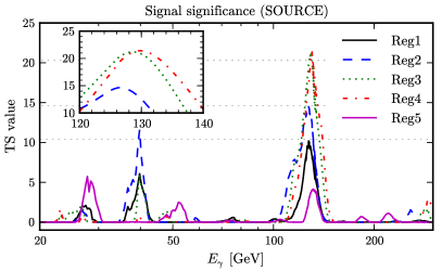
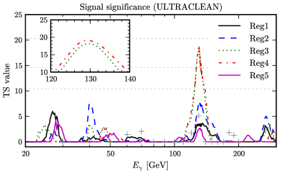
For each of the spectra shown in Fig. 1 we perform a search for gamma-ray lines in the range – as described above. The resulting TS values as function of the gamma-ray line energy are shown in the left and right panels of Fig. 3 for the SOURCE and ULTRACLEAN event classes, respectively. In regions Reg2, Reg3 and Reg4, we find TS values that are surprisingly large, and which indicate a high likelihood for a gamma-ray line at . The largest TS value is obtained in case of the SOURCE events in Reg4 and reads (corresponding to before trial correction). Taking into account the look-elsewhere effect as discussed above, the trial corrected statistical significance for the presence of a line signal in the LAT data is .
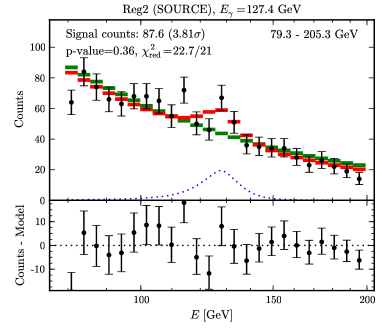
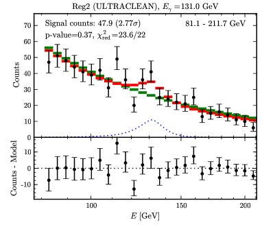
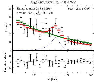
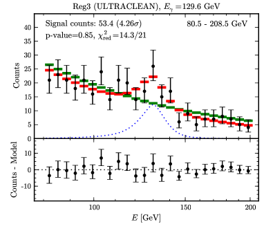
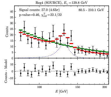
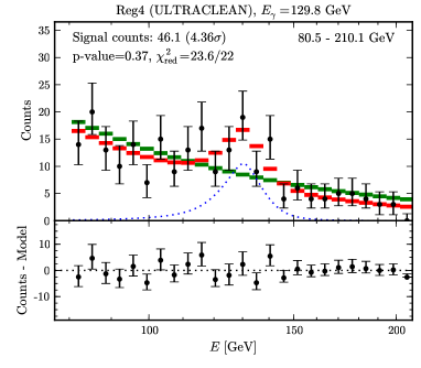
The fits that yield the highest significance for a line contribution are shown in Fig. 4 for the regions Reg2, Reg3 and Reg4, and for SOURCE and ULTRACLEAN events. In the upper sub-panels, we plot the LAT data with statistical error bars, as well as the total predicted counts from the best-fit models with (red bars) and without a gamma-ray line contribution (green bars). The blue dotted line shows the line flux component alone (before averaging over the energy bins). Note that, in order to improve the readability of the plots and to calculate the indicated p-values and the reduced , we rebinned the data to five times fewer bins than actually used in the spectral fits.888In Fig. 4, we omitted incomplete bins at the right end of the energy window. When calculating , we use the c-statistic . The lower sub-panel shows the count residuals after subtracting the model with line. In most of the regions, the spectral signature that is responsible for the large TS values can be easily recognized by eye. The number of signal events ranges between 46 and 88, the statistical significance between and ; the p-values and residual plots confirm that the fits to the data are reasonable and do not exhibit systematic discrepancies at low or high energies.
If we interpret the observed signature as being due to DM annihilation into a photon pair via , we can constrain the DM mass (which then just equals the line energy, ) and the partial annihilation cross-section . The corresponding values for processes like follow from a straightforward rescaling [Vertongen:2011mu]. The inset of Fig. 3 shows a zoom into the most interesting region of the TS plot.999To generate the inset, we did not use sliding energy windows but kept the position of the energy window fixed at the position that corresponds to the with the largest TS. From there, one can read off the DM mass that best fits the data together with its error bars. From the region with the largest TS value, Reg4 SOURCE class, we obtain . The indicated errors are respectively statistical and systematical, the latter being due to uncertainties in the overall energy calibration of the LAT, [Fermi:caveatsPASS7].
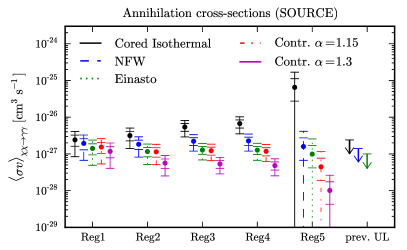
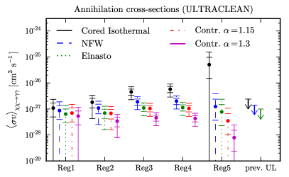
In Fig. 5 we show central values and CL and CL errors for the annihilation cross-section as derived from Reg1 to Reg5, assuming different DM profiles and . We stress that the DM profiles only affect how signal normalizations from the spectral fits translate into annihilation cross-sections, but not the actual spectral analysis itself. In most of the regions, non-zero values of the annihilation cross-section are preferred at more than CL, in agreement with Fig. 3. In case of the cored isothermal or the contracted DM profiles, we find some tension between the annihilation cross-sections obtained from different target regions. In case of the Einasto and NFW profiles, however, the values are mutually consistent. Using SOURCE class events and the spectrum from Reg4, we find best-fit annihilation cross-sections of in case of the Einasto profile, and of in case of the NFW profile. The systematic uncertainties are here derived from the effective area (about [Fermi:caveatsPASS7]) and from the energy calibration.
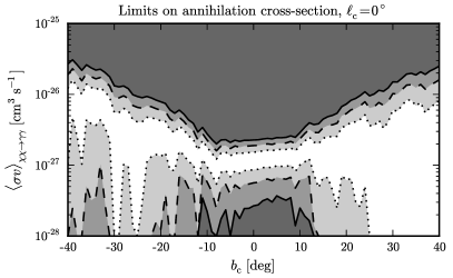
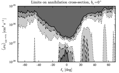
In order to test the locality of the observed signature, we extract the gamma-ray energy spectra from a large number of circular target regions with a radius of . These regions are either centered along the Galactic disk with , or they are centered at from the Galactic north to south pole; and denote the central coordinates of the target regions.101010Note that for these regions are circular with respect to the projection used in Fig. 1. From each of these target regions, we derived the , and CL upper- and lower-limits on the annihilation cross-section , assuming and using the SOURCE event class. As shown in Fig. 6, we find that at CL non-zero values of the annihilation cross-section are only preferred close to the GC; the observed signature disappears when moving to larger values of or .
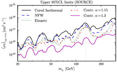
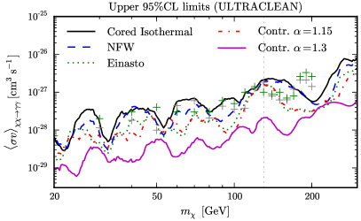
We show CL upper limits on the annihilation cross-section in Fig. 7. For each DM profile, the limits are derived from the correspondingly optimized target region. For all considered DM masses, the presented limits are well below the ‘thermal cross-section’ of . As expected, the limits are weakest in case of the cored isothermal profile, and strongest for the contracted profile with . At a mass around , they show a pronounced bump that corresponds to the large TS values in Fig. 3. For the Einasto profile, we plot previous results from Ref. [Fermi:Symp2011Talk, Edmonds:2011PhD]—based on two years of data without a dedicated target region optimization—as green crosses; except for values around , we improve these limits by factors of two and more.
The signal evidence is based on – photons, cf. Fig. 4. Drawing strong conclusions—in particular on the spatial distribution or the exact spectral shape of the signature—is thus hindered by the low number of events collected so far. Furthermore, our findings could be affected by instrumental systematics, which are difficult to evaluate with public data and information only. However, we checked that obvious systematic uncertainties do not significantly affect our findings; this will be discussed in the next section.
4 Discussion
4.1 Instrumental systematics
Energy reconstruction and line shape. The present analysis is based on the P7SOURCE_V6 and P7ULTRACLEAN_V6 event classes. The corresponding publicly available energy information (CTBBestEnergy) derives from a classification tree analysis of the parametric correction (PC) and shower profile (SP) reconstruction algorithms. With respect to the older event class P6DATACLEAN_V3, PC and SP were debiased; the LK (likelihood) reconstruction algorithm, which was found to introduce jagged peaks that could be mistaken for gamma-ray lines, was removed (see e.g. Ref. [Edmonds:2011PhD]). The data set underlying the present analysis is hence expected to be much better suited for line searches than previously available data.
In previous line searches conducted by the Fermi collaboration (based on the SP energy alone), the spectral shape of reconstructed gamma-ray lines was carefully studied by means of Monte Carlo (MC) simulations that were calibrated with high-energy electron beam tests [Edmonds:2011PhD]; good fits to the MC results were obtained by a superposition of three Gaussians, leading to a peaked line with extended tails. In our analysis, the line shape is derived from the IRF that ships with the ScienceTools; it has a different analytical form, is somewhat broader, and related systematic uncertainties are for us difficult to control. In order to estimate to what extent different spectral line shapes may affect our results, we took the line shape from Fig. 5.3 of Ref. [Edmonds:2011PhD], as well as a simple single Gaussian with a FWHM identical to the one derived from the public IRF (), and used them in the fits. We find that the TS value corresponding to the observed signatures in Reg4 (SOURCE) decreases by 0.7 and 3.0, respectively. The respective best-fit cross-sections are lowered by and . A more careful modeling of the line shape than what we could do in the present work is hence indeed relevant as it obviously affects the results, but it is extremely unlikely that it would invalidate our findings.
Effective area and residual cosmic rays. Uncertainties in the effective area of the LAT have a large point-to-point correlation. On scales corresponding to the width of a gamma-ray line, they are about (and grow to at larger scales) [Fermi:caveatsPASS7]. This is much smaller than the fractional contribution of the observed feature to the overall flux, and can be hence neglected to good approximation. In any case, a sharp line-like feature in the effective area (or residual contamination from the nearly isotropic CRs) would also affect regions of the sky away from the GC. In light of Fig. 6 and the below subsampling analysis, this option appears very unlikely.
Event selection. We checked that the signature appears in both, front- and back-converted ULTRACLEAN events separately, with a higher significance in back-converted events. The signature grew over time, with (8.8, 16.9) when taking only into account only the first 53 (107, 134) weeks of data from Reg3 SOURCE class. Furthermore, we checked that our results remain practically unchanged when using the filter cut DATA_QUAL==1 && IN_SAA!=T && LAT_CONFIG==1 && ABS(ROCK_ANGLE)52 instead, which reduces the number of events by with respect to the adopted DATA_QUAL==1 cut.
4.2 Energy window size
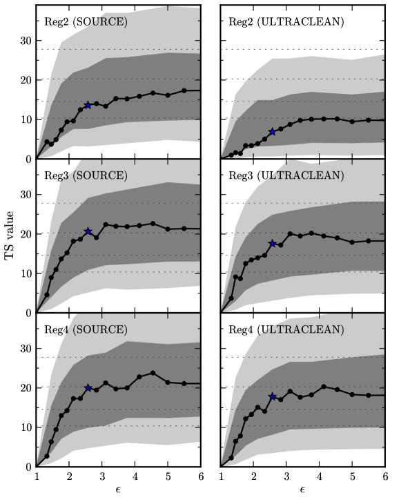
As already discussed above, one critical component in the analysis is the choice of the energy window size. In Fig. 8, the black lines show the TS values obtained when adopting different window sizes , assuming a gamma-ray line energy of . The window borders are given by Eq. (2.6) above, and we show results for Reg2 to Reg4 and SOURCE and ULTRACLEAN events. The window size that we actually used during the main analysis is and indicated by the blue star. As one can see from Fig. 8, an increase of the window size in reasonable ranges leaves the TS values approximately unchanged. On the other hand, a further decrease of the window size would also decreases the TS value. This is expected, because the energy range over which the background normalization is fixed by the data becomes smaller and less constraining in that case.
To study in more detail how well the behaviour of the TS values follows the statistical expectations, we perform a simple MC analysis: For each of the six cases in Fig. 8, we derive the best-fit model with line from an energy window with size . From this model, we generate 400 mock data sets and refit them using smaller windows. The CL and CL bands of the TS values obtained in this way are shown in Fig. 8 by the dark and light shaded gray areas. We find that the actual behaviour of the observed TS value as function of follows very well the MC results. This supports our choice of a window size of at . Smaller windows would significantly decrease the statistical power of the analysis.
Lastly, we checked that fixing the slope of the background power-law to (2.5, 2.7) results in TS values of 20.4 (19.4, 21.5) in case of Reg4 (SOURCE); this again has little impact on our findings. A value of is physically expected since the gamma-ray flux in Reg4 is dominated by diffuse photons from cosmic-ray proton collisions with the interstellar medium.
4.3 Monte Carlo and subsampling analysis
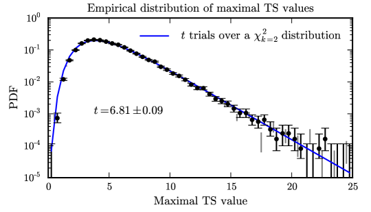
In order to estimate the statistical significance of the observed excess, we perform a simple Monte Carlo analysis of our line search. We generate 25000 mock spectra that follow a power-law with slope (like in Reg1 SOURCE class), such that each mock data set has the same number of counts as observed in Reg3 SOURCE. In each of these spectra, we perform the above spectral analysis, and record the corresponding largest TS value. The distribution of these maximal TS values is shown by the black dots in Fig. 9 with statistical error bars. We fit this distribution with the probability distribution function (PDF) of the maximum from trials over a distribution, which reads
| (4.1) |
leaving as free parameters in the fit. Note that our corresponds to the ’effective number of search regions’ discussed in Ref. [Gross:2010qma] (related to the number of upcrossings), and is in our case the theoretical expectation for the tail of the distribution. Since we are mainly interested in this distribution tail, we only take TS values above 5 into account in the fit. However, as shown in Fig. 9 by the blue line, we find that trials well reproduce the empirical result over the whole range. We checked that increasing/decreasing the energy window or sample size within reasonable values does not change these results.
In order to confirm the above Monte Carlo results with real data, we perform a subsampling analysis of the LAT data in regions where no signal is expected. To this end, we exclude all data from the hemisphere towards the GC. The events from the region away from the GC, and , are distributed in energy bins , the number of events in each energy bin is called . From these we generate 21000 test spectra; the expectation value for each energy bin is given by . The small prefactor ensures that statistical fluctuations within the original data do not destroy the tail distribution of the subsampling analysis. Like above, we record for each of the test spectra the largest TS value found. The results are shown in Fig. 9 by the gray bands (which indicate the statistical error bars). They are in excellent agreement with the Monte Carlo results. We checked that this agreement does not strongly depend on the energy window size or on the above prefactor; it holds in particular also in the case where the number of events per test spectra equals the number of events in Reg3.
We emphasize that line-like artefacts in the effective area of the LAT or contamination with isotropic cosmic rays would most likely have shown up as disagreement between our Monte Carlo and subsampling results, since they should also affect the fluxes observed towards the anti-galactic center.
4.4 Comparison with previous results
The strongest previously presented upper limits on gamma-ray lines at an energy of read for an NFW (Einasto, cored isothermal) DM profile (at CL) [Fermi:Symp2011Talk, Edmonds:2011PhD], and are based on two years of data and an analysis of a large sky region. In case of the Einasto profile, these limits are marginally consistent with the different best-fit cross-section that we show in Fig. 5. In case of the NFW (cored isothermal) profile, however, there is a two sigma tension between previous limits and the best-fit value from Reg4. This could be read as a weak preference for the Einasto (or for a compressed) DM profile. However, it could also indicate systematics related e.g. to the shape of the gamma-ray line that biases the obtained cross-sections to high, or it could be due to statistical fluctuations in the different underlying data sets. In any case, these limits would set interesting and complementary constraints on the allowed DM profiles if the 130 GeV signature is due to DM annihilation.
In Refs. [Fermi:Symp2011Talk, Edmonds:2011PhD], which is based on the SP energy only, the significance for a signal at was found to be . As a test whether this conflicts with our results, we implemented the target region and energy windows from Refs. [Fermi:Symp2011Talk, Edmonds:2011PhD] (without doing a point-source subtraction), and repeated their scan over the discrete line energies , using 43 months of ULTRACLEAN data. In this way, we find the TS values (upper limits) that are shown by the gray crosses in the right panel of Fig. 3 (Fig. 7). Indeed, no strong indication for a signature at 130 GeV appears, whereas the resulting limits are in good agreement with—and slightly stronger than—the two-years results from [Fermi:Symp2011Talk, Edmonds:2011PhD]. This illustrates that a continuous scan over of gamma-ray line energies, a careful selection of energy windows and an improved selection of target regions is extremely important when searching for very faint signatures.
5 Conclusions
We presented a refined search for gamma-ray lines with the Fermi Large Area Telescope. The main improvement with respect to previous analyses is the use of a new optimization algorithm that automatically selects target regions with the largest signal-to-noise ratio, depending on the adopted Galactic dark matter profile and the LAT data. Besides, we updated previous results to 43 months of data and used the most recent public event selection.
We found a indication for the presence of a gamma-ray line at .111111We reported this signature before in Ref. [Bringmann:2012vr] in context of internal Bremsstrahlung signals from DM. Taking into account the look-elsewhere effect, the significance is . By scanning through different regions of the sky, we find that the signature appears close to the Galactic center only. If interpreted in terms of dark matter annihilation into photon pairs, , the observations constrain the dark matter mass to . The annihilation cross-sections derived from different target regions are consistent with each other in the case of the Einasto or NFW dark matter profiles. For these, we obtain best-fit annihilation cross-sections of and , respectively. Assuming a thermal relic, this corresponds to a branching ratio into final states of –, which is much larger than what the generic one-loop suppression suggests. We examined our statistical method with Monte Carlo methods and with a subsampling analysis of the LAT data in the hemisphere, and find good agreement with theoretical expectations. We performed several checks to exclude that obvious systematics of the LAT could invalidate our findings. In particular the fact that the signal peaks around the Galactic center makes a purely instrumental cause very unlikely.
The observation of a gamma-ray line from dark matter annihilation in the data of the Fermi LAT is a fascinating possibility. However, a few caveats are in order. First, the presented analysis is based on publicly available data and information only, hence we cannot take into account all possible instrumental effects. Second, the signal evidence is right now based on around photons; it will require a few years of more data to settle its existence on statistical grounds. Third, due to the low number of events it is difficult to study in detail the spatial and spectral characteristics of the signature, which might still leave room for some exotic astrophysical explanation.
In any case, we showed that a careful selection of target regions is extremely important when searching for gamma-ray lines. We hope that our work motivates a refined search for such features in the Fermi LAT data, including all instrumental effects, an improved event selection and a target region optimization as proposed in this paper.
Acknowledgments.
I am very grateful to Torsten Bringmann, Ilias Cholis, Michael Gustafsson, Dieter Horns, Luca Maccione, David Paneque, Maksim Pshirkov, Georg Raffelt, Javier Redondo and Stefan Vogl for useful comments on the manuscript and valuable discussion about the Fermi LAT and statistical methods. I acknowledges partial support from the European 1231 Union FP7 ITN INVISIBLES (Marie Curie Actions, PITN-GA-2011-289442). This work makes use of SciPy [SciPy], PyFITS121212http://www.stsci.edu/resources/software_hardware/pyfits, PyMinuit131313http://code.google.com/p/pyminuit and IPython [IPython].
Note added.
After submission of this manuscript, the two-years line search of the LAT collaboration was released [Ackermann:2012qk]. The results were already presented on different conferences during last year [Fermi:Symp2011Talk], details can be found in Ref. [Edmonds:2011PhD]. We comment on them where appropriate.
Appendix A Event Tables
| bins | #Counts | #Signal | Flux |
|---|---|---|---|
| 79.3–82.4 | 64 | 0.34 | 1.37e-10 |
| 82.4–85.6 | 84 | 0.42 | 1.73e-10 |
| 85.6–89.0 | 74 | 0.53 | 1.47e-10 |
| 89.0–92.5 | 66 | 0.68 | 1.27e-10 |
| 92.5–96.1 | 63 | 0.88 | 1.17e-10 |
| 96.1–99.8 | 68 | 1.17 | 1.22e-10 |
| 99.8–103.7 | 68 | 1.61 | 1.18e-10 |
| 103.7–107.8 | 65 | 2.31 | 1.09e-10 |
| 107.8–112.0 | 55 | 3.54 | 8.88e-11 |
| 112.0–116.4 | 72 | 5.81 | 1.12e-10 |
| 116.4–120.9 | 50 | 9.68 | 7.53e-11 |
| 120.9–125.7 | 46 | 15.18 | 6.7e-11 |
| 125.7–130.6 | 67 | 18.89 | 9.43e-11 |
| 130.6–135.7 | 51 | 13.76 | 6.94e-11 |
| 135.7–141.0 | 36 | 7.07 | 4.74e-11 |
| 141.0–146.5 | 35 | 3.04 | 4.45e-11 |
| 146.5–152.2 | 34 | 1.30 | 4.18e-11 |
| 152.2–158.2 | 34 | 0.61 | 4.04e-11 |
| 158.2–164.4 | 28 | 0.34 | 3.22e-11 |
| 164.4–170.8 | 23 | 0.20 | 2.56e-11 |
| 170.8–177.5 | 26 | 0.12 | 2.79e-11 |
| 177.5–184.4 | 22 | 0.07 | 2.29e-11 |
| 184.4–191.6 | 19 | 0.04 | 1.91e-11 |
| 191.6–199.1 | 14 | 0.03 | 1.36e-11 |
| bins | #Counts | #Signal | Flux |
|---|---|---|---|
| 81.1–84.3 | 47 | 0.16 | 9.39e-11 |
| 84.3–87.6 | 51 | 0.20 | 9.83e-11 |
| 87.6–91.0 | 48 | 0.25 | 8.94e-11 |
| 91.0–94.6 | 44 | 0.33 | 7.91e-11 |
| 94.6–98.3 | 41 | 0.43 | 7.12e-11 |
| 98.3–102.1 | 39 | 0.58 | 6.55e-11 |
| 102.1–106.1 | 42 | 0.81 | 6.8e-11 |
| 106.1–110.3 | 31 | 1.16 | 4.84e-11 |
| 110.3–114.6 | 49 | 1.78 | 7.37e-11 |
| 114.6–119.1 | 36 | 2.94 | 5.23e-11 |
| 119.1–123.7 | 20 | 4.96 | 2.81e-11 |
| 123.7–128.6 | 36 | 7.99 | 4.9e-11 |
| 128.6–133.6 | 41 | 10.57 | 5.39e-11 |
| 133.6–138.8 | 25 | 8.16 | 3.18e-11 |
| 138.8–144.3 | 24 | 4.25 | 2.95e-11 |
| 144.3–149.9 | 22 | 1.82 | 2.62e-11 |
| 149.9–155.8 | 21 | 0.76 | 2.41e-11 |
| 155.8–161.9 | 25 | 0.35 | 2.77e-11 |
| 161.9–168.2 | 13 | 0.18 | 1.39e-11 |
| 168.2–174.8 | 15 | 0.10 | 1.55e-11 |
| 174.8–181.6 | 16 | 0.06 | 1.59e-11 |
| 181.6–188.7 | 14 | 0.04 | 1.35e-11 |
| 188.7–196.1 | 11 | 0.02 | 1.03e-11 |
| 196.1–203.8 | 10 | 0.01 | 9.02e-12 |
| 203.8–211.7 | 6 | 0.01 | 5.24e-12 |
| bins | #Counts | #Signal | Flux |
|---|---|---|---|
| 80.5–83.7 | 21 | 0.18 | 2.03e-10 |
| 83.7–86.9 | 23 | 0.23 | 2.14e-10 |
| 86.9–90.3 | 21 | 0.29 | 1.89e-10 |
| 90.3–93.9 | 18 | 0.37 | 1.56e-10 |
| 93.9–97.6 | 21 | 0.49 | 1.76e-10 |
| 97.6–101.4 | 16 | 0.66 | 1.3e-10 |
| 101.4–105.3 | 24 | 0.92 | 1.88e-10 |
| 105.3–109.5 | 14 | 1.34 | 1.06e-10 |
| 109.5–113.7 | 21 | 2.06 | 1.53e-10 |
| 113.7–118.2 | 20 | 3.41 | 1.4e-10 |
| 118.2–122.8 | 14 | 5.76 | 9.49e-11 |
| 122.8–127.6 | 17 | 9.21 | 1.11e-10 |
| 127.6–132.6 | 26 | 11.80 | 1.65e-10 |
| 132.6–137.8 | 15 | 8.72 | 9.2e-11 |
| 137.8–143.2 | 17 | 4.45 | 1.01e-10 |
| 143.2–148.8 | 6 | 1.89 | 3.44e-11 |
| 148.8–154.6 | 9 | 0.79 | 4.98e-11 |
| 154.6–160.6 | 5 | 0.36 | 2.67e-11 |
| 160.6–166.9 | 7 | 0.19 | 3.61e-11 |
| 166.9–173.4 | 7 | 0.11 | 3.48e-11 |
| 173.4–180.2 | 8 | 0.07 | 3.84e-11 |
| 180.2–187.3 | 7 | 0.04 | 3.25e-11 |
| 187.3–194.6 | 5 | 0.02 | 2.25e-11 |
| 194.6–202.2 | 4 | 0.01 | 1.74e-11 |
| bins | #Counts | #Signal | Flux |
|---|---|---|---|
| 80.5–83.7 | 14 | 0.15 | 2.31e-10 |
| 83.7–86.9 | 20 | 0.19 | 3.18e-10 |
| 86.9–90.3 | 13 | 0.25 | 1.99e-10 |
| 90.3–93.9 | 10 | 0.32 | 1.48e-10 |
| 93.9–97.6 | 14 | 0.42 | 2e-10 |
| 97.6–101.4 | 7 | 0.57 | 9.68e-11 |
| 101.4–105.3 | 15 | 0.79 | 2e-10 |
| 105.3–109.5 | 9 | 1.14 | 1.16e-10 |
| 109.5–113.7 | 13 | 1.75 | 1.61e-10 |
| 113.7–118.2 | 17 | 2.88 | 2.04e-10 |
| 118.2–122.8 | 9 | 4.87 | 1.04e-10 |
| 122.8–127.6 | 13 | 7.81 | 1.46e-10 |
| 127.6–132.6 | 19 | 10.18 | 2.06e-10 |
| 132.6–137.8 | 9 | 7.68 | 9.42e-11 |
| 137.8–143.2 | 15 | 3.96 | 1.52e-10 |
| 143.2–148.8 | 4 | 1.69 | 3.92e-11 |
| 148.8–154.6 | 6 | 0.70 | 5.67e-11 |
| 154.6–160.6 | 4 | 0.32 | 3.65e-11 |
| 160.6–166.9 | 4 | 0.17 | 3.52e-11 |
| 166.9–173.4 | 5 | 0.10 | 4.24e-11 |
| 173.4–180.2 | 5 | 0.06 | 4.09e-11 |
| 180.2–187.3 | 4 | 0.03 | 3.17e-11 |
| 187.3–194.6 | 3 | 0.02 | 2.3e-11 |
| 194.6–202.2 | 3 | 0.01 | 2.22e-11 |
| 202.2–210.1 | 0 | 0.01 | 0 |