Minimal and Robust Composite Two-Qubit Gates with Ising-Type Interaction

Abstract

We construct a minimal robust controlled-NOT gate with an Ising-type interaction by which elementary two-qubit gates are implemented. It is robust against inaccuracy of the coupling strength and the obtained quantum circuits are constructed with the minimal number ($N=3$) of elementary two-qubit gates and several one-qubit gates. It is noteworthy that all the robust circuits can be mapped to one-qubit circuits robust against a pulse length error. We also prove that a minimal robust SWAP gate cannot be constructed with $N=3$, but requires $N=6$ elementary two-qubit gates.

I Introduction

Gates robust against noise are essential for reliable computation irrespective of its nature being classical or quantum Feynman96 ; NC00 ; Gaitan07 ; NO08 . In quantum computation, one of the promising ways to achieve this goal is to employ composite gates Jones11 ; Jones09 : Realizing a target gate as a sequence of elementary gates so that systematic errors inherent in elementary gates cancel with each other.

It has been becoming clear that one must pay attention to both the noise and systematic errors, so as to materialize a working quantum computer. Indeed, in a layered architecture for quantum computing, physical qubits undergo the composite gate operations and dynamical decoupling as preliminary processing to quantum error correction, which compensates for bit flips and phase flips due to the stochastic noise CodyJones12 .

Composite gates (pulses) have been developed in nuclear magnetic resonance (NMR), which is also a good test bed for quantum computation. Operations in NMR are implemented with the following elementary unitary gates:

$$R(\theta,\phi) = \exp[-i\theta(\cos\phi\sigma_{x}+\sin\phi\sigma_{y})/2],$$

$$S(\Theta) = \exp(-i\Theta\sigma_{z}\otimes\sigma_{z}/4),$$ (1)

where $\sigma_{i}\ (i=x,y,z)$ are the Pauli matrices. We will consider quantum circuits made of these gates (1). The operations $R(\theta,\phi)$’s are realized with so-called rf-pulses, while $S(\Theta)$’s are implemented by free evolutions of a system under the Hamiltonian $J\sum_{i}\sigma_{i}\otimes\sigma_{i}/4$ that becomes the Ising-type interaction $J\sigma_{z}\otimes\sigma_{z}/4$ in the weak coupling limit Levitt . Hereafter we assume $J>0$ so that $\Theta=JT\geq 0$, where $T\geq 0$ is the execution time required to implement $S(\Theta)$.

Any multi-qubit unitary operations can be written as quantum circuits composed of one-qubit unitary gates and the controlled-NOT (CNOT) gates Barenco95 . For one-qubit gates in liquid-state NMR quantum computation, the most important systematic errors are pulse length errors and off-resonance errors Jones09 . These errors are suppressed with composite one-qubit gates Alway07 ; Ichikawa11 ; Bando12 . The remaining task is to construct robust two-qubit gates.

For two-qubit gates, an error in the parameter $\Theta$ must be considered. This error may be caused by (1) inaccuracy of the numerical value of the coupling $J$ or (2) influence of other qubits. It might be caused by an error in gate execution time $T$, too. Many composite gates have been proposed to suppress this error Jones03 ; phtr ; Hill07 ; Testolin07 ; Tomita10 . The composite gates proposed in Jones03 compensates for the error terms for $S(\Theta)$ up to the second order, whereas those proposed in Hill07 are applicable to more general interactions. However, these merits are realized at the cost of longer execution time, which leads to less tolerance to stochastic noise: Shorter composite pulse is desirable.

All these two-qubit composite gates are designed following the idea that any one-qubit quantum circuit robust against the pulse length error is mapped to a two-qubit composite gate robust against the error in $\Theta$. The mathematical basis of this approach is that ${\rm SU}(2)$ may be mapped to a proper subgroup of ${\rm SU}(4)$. Although this approach was successful, we might have ruled out robust two-qubit gates that have no corresponding one-qubit gates.

In this paper, we start from the most generic quantum circuit for a two-qubit gate in NMR quantum computation depicted in Fig. 1. Then, we construct minimal robust composite two-qubit gates. We claim our gates are “minimal” in that the obtained quantum circuits are constructed with a minimal number of two-qubit gates. Moreover, it will be shown below that all our minimal robust composite two-qubit gates have the corresponding one-qubit composite gates.

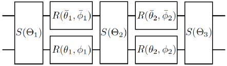
Figure 1: Schematic diagram of the quantum circuit (2) for $N=3$. $R(\theta_{i},\phi_{i})$ and $S(\Theta_{i})$ are defined by Eq. (1).

This paper is organized as follows. In Sec. II, we introduce a circuit family that we are going to analyze. A robustness condition is also derived. In Sec. III, we apply it to the circuit family and obtain the simplest exact solutions. This solution realizes the robust CNOT gates, but not the robust SWAP gates. However, we will find a suitable combination of the solutions, which makes the robust gates equivalent to the SWAP gates up to one-qubit gates. In Sec. IV, we demonstrate an intriguing property of the solutions. All the composite two-qubit gates designed with our solutions have correspondence to one-qubit composite gates. By using this, we show that the solutions can be seen as extensions of well-known one-qubit composite gates. Section V is devoted to conclusion and discussions.

II Robustness Conditions

Consider a circuit which implements the following unitary operation,

$$U = S_{N}(\bar{R}_{N-1}\otimes R_{N-1})S_{N-1}\cdots(\bar{R}_{1}\otimes R_{1})S_{1},$$ (2)

where $R_{i}=R(\theta_{i},\phi_{i})$, $\bar{R}_{i}=R(\bar{\theta}_{i},\bar{\phi}_{i})$ and $S_{i}=S(\Theta_{i})$. For this circuit, we discuss a systematic error in $S(\Theta)$ so that the real one is given by

$$S^{\prime}_{j}=S^{\prime}(\Theta_{j})=S\left((1+\epsilon)\Theta_{j}\right),$$ (3)

where $\epsilon\in\mathbb{R}$ quantifies error magnitude. We assume here that all the one-qubit gates $R_{j}$ ($\bar{R}_{j}$) in Fig. 1 are implemented instantaneously and error-free, since we can employ robust one-qubit gates Alway07 ; Ichikawa11 ; Bando12 . On these assumptions, the circuit we actually implement is no longer $U$, but

$$U^{\prime} = S_{N}^{\prime}(\bar{R}_{N-1}\otimes R_{N-1})S_{N-1}^{\prime}\cdots(\bar{R}_{1}\otimes R_{1})S_{1}^{\prime}.$$ (4)

In practice, the error strength is unknown but assumed to be reasonably small so that the perturbation theory is applicable ($|\epsilon|\ll 1$). Therefore, we may expand $U^{\prime}$ as

$${U}^{\prime}=U-i\epsilon\delta U+{\cal O}(\epsilon^{2}).$$ (5)

We require the condition

$$\delta U=0$$ (6)

for $U^{\prime}$ to be robust against the error up to the first order in $\epsilon$ and call this condition the robustness condition for $U$. Note that $U$ and $(\bar{R}_{N}\otimes R_{N})U(\bar{R}_{0}\otimes R_{0})$ have the same robustness since all the one-qubit gates are assumed to be error-free.

III Robust Circuits

We will construct minimal circuits that implement nontrivial robust two-qubit gates. We are especially interested in a robust $S(\Theta)$ gate required to implement the CNOT gate.

III.1 No Robust Entanglers with $N$=2

Let us begin our analysis with the case $N=2$, which is the simplest one in terms of the circuit complexity. To derive the explicit form of the robustness condition (6), let us approximate $S^{\prime}_{j}=(1-i\epsilon\Theta_{j}\sigma_{z}\otimes\sigma_{z}/4)S_{j}$ to the first order in $\epsilon$. Substituting this to Eq. (4) and using $R_{i}\sigma_{z}=\sigma_{z}R_{i}^{\dagger}$, we find

$$\delta U = \frac{1}{4}\left[\Theta_{2}\sigma_{z}^{\otimes 2}S_{2}(\bar{R}_{1}\otimes R_{1})S_{1}+\Theta_{1}S_{2}(\bar{R}_{1}\otimes R_{1})\sigma_{z}^{\otimes 2}S_{1}\right]$$ (7)

$$= \frac{1}{4}\sigma_{z}^{\otimes 2}S_{2}\left(\Theta_{2}\bar{R}_{1}\otimes R_{1}+\Theta_{1}\bar{R}_{1}^{\dagger}\otimes R_{1}^{\dagger}\right)S_{1}.$$

Thus, the robustness condition (6) reduces to

$$\Theta_{2}(\bar{R}_{1}\otimes R_{1})^{2}+\Theta_{1}\openone^{\otimes 2}=0,$$ (8)

where $\openone$ is the $2\times 2$ identity matrix. The solution is $\bar{R}_{1}^{2}\otimes R_{1}^{2}=\pm\openone^{\otimes 2}$ with $\Theta_{1}/\Theta_{2}=\mp 1$. Then $U=\pm\bar{R}_{1}\otimes R_{1}$, which implies that all the robust circuits belong to $\rm{SU}(2)^{\otimes 2}$. This proves that a robust $S(\Theta)$ for generic $\Theta$ with $N=2$ is impossible. We should try $N\geq 3$ to implement a non-trivial two-qubit gate robust against the error in $\Theta$.

III.2 Minimal Robust Entangler with $N$=3

The error term $\delta U$ for $N=3$ is written explicitly as

$$\delta U = \frac{1}{4}[\Theta_{1}\sigma_{z}^{\otimes 2}S_{1}(\bar{R}_{1}\otimes R_{1})S_{2}(\bar{R}_{2}\otimes R_{2})S_{3}$$ (9)

$$+ \Theta_{2}S_{1}(\bar{R}_{1}\otimes R_{1})\sigma_{z}^{\otimes 2}S_{2}(\bar{R}_{2}\otimes R_{2})S_{3}$$

$$+ \Theta_{3}S_{1}(\bar{R}_{1}\otimes R_{1})S_{2}(\bar{R}_{2}\otimes R_{2})\sigma_{z}^{\otimes 2}S_{3}].$$

Similarly to the $N=2$ case, by using $R_{i}\sigma_{z}=\sigma_{z}R_{i}^{\dagger}$, the robustness condition (6) reads

$$\Theta_{3}(\bar{R}_{2}\otimes R_{2})^{2}+\Theta_{2}\openone^{\otimes 2}+\Theta_{1}S_{2}(\bar{R}_{1}^{\dagger}\otimes R_{1}^{\dagger})^{2}S_{2}^{\dagger}=0.$$ (10)

We set $\phi_{2}=\bar{\phi}_{2}=0$ without loss of generality since we can apply $e^{i\bar{\xi}\sigma_{z}}\otimes e^{i\xi\sigma_{z}}$ to $U$ and freely adjust $\phi_{2}$ and $\bar{\phi}_{2}$ without changing the robustness condition. The robustness condition (10) reduces to

$$\Theta_{3}\bar{c}_{2}c_{2} = -\Theta_{2}-\Theta_{1}\bar{c}_{1}c_{1},$$ (11a)

$$e^{-i\phi_{1}}\Theta_{3}\bar{s}_{2}s_{2} = -e^{i\bar{\phi}_{1}}\,\Theta_{1}\bar{s}_{1}s_{1}=-e^{-i\bar{\phi}_{1}}\,\Theta_{1}\bar{s}_{1}s_{1},$$ (11b)

$$e^{-i\phi_{1}}\Theta_{3}\bar{c}_{2}s_{2} = e^{i\Theta_{2}/2}\,\Theta_{1}\bar{c}_{1}s_{1}=e^{-i\Theta_{2}/2}\Theta_{1}\,\bar{c}_{1}s_{1},$$ (11c)

$$e^{i\bar{\phi}_{1}}\Theta_{3}\bar{s}_{2}c_{2} = e^{i\Theta_{2}/2}\Theta_{1}\,\bar{s}_{1}c_{1}=e^{-i\Theta_{2}/2}\Theta_{1}\,\bar{s}_{1}c_{1},$$ (11d)

where we introduced $c_{i}=\cos\theta_{i}$, $\bar{c}_{i}=\cos\bar{\theta}_{i}$, $s_{i}=\sin\theta_{i}$, $\bar{s}_{i}=\sin\bar{\theta}_{i}$ for $i=1,2$. General solutions of Eqs. (11) are

$$\phi_{1}=\phi_{2}= \bar{\phi}_{1} =\bar{\phi}_{2}=0,$$

$$\bar{\theta}_{1}\equiv\bar{\theta}_{2}\equiv 0\pmod{\pi}, \Theta_{2}\equiv 0\pmod{2\pi},$$

$$\Theta_{1}=\frac{\alpha\Theta_{2}\sin\theta_{2}}{\sin(\gamma\theta_{1}+\theta_{2})}, \Theta_{3}=\frac{\beta\Theta_{2}\sin\theta_{1}}{\sin(\gamma\theta_{1}+\theta_{2})}.$$ (12)

For brevity, we introduced symbols $\alpha,\beta,\gamma\in\{\pm 1\}$, which are determined by $\bar{\theta}_{1},\bar{\theta}_{2}$ and $\Theta_{2}$ (See TABLE 1). Derivation of the above solution is given in the Appendix. Note that $\Theta_{2}\neq 0$ for $U=S(\Theta)$ to be nontrivial. We list the properties of the solution (12): First, the axes of the one-qubit gates are aligned: $\phi_{i}=\bar{\phi}_{i}=0$. Second, this circuit has the shortest execution time when $\Theta_{2}=2\pi$, since the execution time $T$ is proportional to $\sum_{i=1}^{3}|\Theta_{i}|\propto|\Theta_{2}|$. We also obtain the other class of general solutions by renaming the qubits as $1\leftrightarrow 2$.

Table 1: Two-value variables $\alpha,\beta,\gamma\in\{\pm 1\}$ in Eq. (12) as functions of $\bar{\theta}_{1},\bar{\theta}_{2},\Theta_{2}$. Note that $\Theta_{2}\neq 0$.

$\alpha$	$\bar{\theta}_{1}/\pi$
1	odd
$-1$	even

$\beta$	$\bar{\theta}_{2}/\pi$
$\gamma$	odd
$-\gamma$	even

$\gamma$	$\Theta_{2}/2\pi$
1	even
$-1$	odd

The general solutions (12) are apparently complicated due to various combinations of $\alpha,\beta$ and $\gamma$. Nevertheless, the solution can be simplified, without loss of generality, as follows. Let us note that

$$(\sigma_{x}\otimes\openone)S\left(\Theta_{1}\right)|_{\alpha}(\sigma_{x}\otimes\openone)=S\left(\Theta_{1}\right)|_{-\alpha}.$$ (13)

We can freely flip $\alpha$ with the one-qubit unitary operations. By noting that $\bar{R}_{1}=\pm i\sigma_{x}$ for $\alpha=1$ and $\bar{R}_{1}=\pm\openone$ for $\alpha=-1$, we can eliminate $\bar{R}_{1}$ by taking $\alpha=-1$. Similar observation applies to $\beta$ as well: $\bar{R}_{2}=\pm i\sigma_{x}$ for $\beta=\gamma$ and $\bar{R}_{2}=\pm\openone$ for $\beta=-\gamma$. Thus, we can always take $\alpha=-1$, $\beta=-\gamma$ and the resulting circuit has the minimal number of elementary gates as shown in Fig. 2. We will work with this circuit from now on.

We present the simplest, and thus the most useful, example that implements a composite gate $U=S(\Theta)$ for an arbitrary $\Theta$. First, let us take $\Theta_{2}=2\pi$ so that the execution time is shortest and $\gamma=-1$. We then take $\bar{\theta}_{1}=\bar{\theta}_{2}=0$ to ensure $\alpha=-1$ and $\beta=-\gamma(=1)$. Further we put $-\theta_{1}=\theta_{2}=\theta\in[\pi/2,\pi]$, where $\theta$ is a parameter chosen in such a way that $\Theta_{1}=\Theta_{3}=-\pi\sec\theta\geq 0$ and that $R_{1},R_{2}$ are the shortest pulses. For this simplest composite pulse $U$, we find the identity

$$[\openone\otimes R(\eta,0)]U[\openone\otimes R(\eta,0)]^{\dagger}=S(4\zeta),$$ (14)

where $\eta$ and $\zeta$ are given by

$$\tan\eta = \tan\theta\sec\left(\frac{\pi}{2}\sec\theta\right),$$

$$\cos\zeta = \cos\theta\sin\left(\frac{\pi}{2}\sec\theta\right).$$ (15)

Thus, up to one-qubit unitary operations, $U$ implements the operation $S(\pi)$ ($\zeta=\pi/4$). Since the Cartan decomposition of the CNOT gate contains $S(\pi)$ NO08 , we observe that $U$ implements the robust CNOT gate. In case of the shortest pulse, this operation is realized by taking

$$\theta=\pi-\theta^{\star},\qquad\theta^{\star}\approx 0.674,$$ (16)

which has been obtained by solving the second equation of Eqs. (15) numerically with $\zeta=\pi/4$.

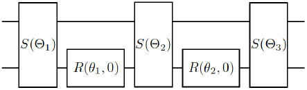
Figure 2: Schematic diagram of the minimal robust circuit ($N=3$, $\alpha=-1,\beta=-\gamma$).

This simplest circuit, however, does not implement the SWAP gate. Note that

$$S(4\zeta)=\cos\zeta\openone^{\otimes 2}-i\sin\zeta\sigma_{z}^{\otimes 2},$$ (17)

while

$${\rm SWAP} = \left(\begin{array}[]{cccc}1&0&0&0\\ 0&0&1&0\\ 0&1&0&0\\ 0&0&0&1\end{array}\right)=\frac{\openone^{\otimes 2}+\sigma_{x}^{\otimes 2}+\sigma_{y}^{\otimes 2}+\sigma_{z}^{\otimes 2}}{2}.$$ (22)

Since any one-qubit unitary operations leave the number of the summand in the right hand side unchanged, $S(4\zeta)$ cannot be converted to the SWAP gate, which proves our claim More precise argument is as follows: First, note that $\{\openone,\sigma_{x},\sigma_{y},\sigma_{z}\}$ forms an orthogonal basis, in the sense of the Hilbert-Schmidt inner product. By one-qubit unitary transformations, the orthonormal basis undergoes the change $\{\openone,\sigma_{x},\sigma_{y},\sigma_{z}\}^{\otimes 2}\to V_{1}\{\openone,\sigma_{x},\sigma_{y},\sigma_{z}\}W_{1}\otimes V_{2}\{\openone,\sigma_{x},\sigma_{y},\sigma_{z}\}W_{2}$, where $V_{i},W_{i}\in$ SU(2). The new bases $V_{i}\{\openone,\sigma_{x},\sigma_{y},\sigma_{z}\}W_{i}$ are also orthogonal bases. We use these transformed bases to evaluate the number of summands after the one-qubit unitary operations. Note that this can be also shown by using operator Schmidt decomposition Nielsen00 ; Nielsen03 or SU(2)^⊗2 invariants Makhlin02 ; Zhang03 ; Zhang04 . The above observation is proven to be valid also for the general solutions (12): The $N=3$ general solutions generate the robust composite pulses for $S(\Theta)$ only, while there are no such $N=3$ solutions that make the SWAP gate robust.

III.3 Minimal Robust SWAP Gates

Instead of the SWAP gate, let us consider how to make a composite gate of the following 2-qubit gate

$$V = \left(\begin{array}[]{cccc}1&0&0&0\\ 0&0&-i&0\\ 0&-i&0&0\\ 0&0&0&1\end{array}\right)=\frac{\openone^{\otimes 2}-i\sigma_{x}^{\otimes 2}-i\sigma_{y}^{\otimes 2}+\sigma_{z}^{\otimes 2}}{2}.$$ (28)

To investigate the properties of $V$, let us introduce operator Schmidt coefficients (OSCs) and operator Schmidt number (OSN). The OSCs are coefficients of the basis operators appearing after the operator Schmidt decomposition is carried out. The OSN stands for the number of the non-zero OSCs Nielsen00 ; Nielsen03 . Note that both the OSCs and OSN are local unitary (LU) invariants. This implies that if the OSNs of given two operators are different from each other, then two operators cannot be locally equivalent.

By using the OSCs, we find that the $V$ gate is LU equivalent to the SWAP gate, since the OSCs of $V$ are $\{1/2,1/2,1/2,1/2\}$, which are identical to those of the SWAP gates as shown in Eq. (LABEL:swapmat). Thus we may identify the $V$ gate with the SWAP gate, up to LU operations.

Now let us evaluate how many elementary $S(\Theta)$ gates we need in order to construct the $V$ gate. Clearly it is impossible to construct the $V$ gate (and hence the SWAP gate) with only one elementary $S(\Theta)$ gate, as shown in the previous section. We can construct the $V$ gate with two elementary $S(\pi)$ gates as

$$V = R\left(\tfrac{\pi}{2},\tfrac{\pi}{2}\right)^{\otimes 2}S(\pi)[R\left(\tfrac{\pi}{2},\tfrac{\pi}{2}\right)^{\otimes 2}]^{\dagger}$$ (30)

$$\times R\left(\tfrac{\pi}{2},0\right)^{\otimes 2}S(\pi)[R\left(\tfrac{\pi}{2},0\right)^{\otimes 2}]^{\dagger},$$

which is a minimal circuit of $V$ within the gate set (1). By replacing two elementary $S(\pi)$ gates in Eq. (30) by the $N=3$ composite $S(\pi)$ gates (14), we find the $N=2\times 3=6$ robust $V$ gate.

Let us check whether there are smaller constructions of a robust $V$ gate based on the circuit (30). According to Sec. III.1, any $N=2$ robust gate implements the trivial gate only. Thus, taking into account the fact that the two factors the right hand side of Eq. (30) implement non-trivial entangling gates, it turns out that we must use two $N=3$ solutions (14) for the robust implementation of $V$, totaling 6 elementary $S(\pi)$ gates. Furthermore, we find that in the resulting robust $V$ circuit, the sub-circuit starting from the third elementary $S(\Theta)$ gate to the fourth cannot be merged to a single elementary $S(\Theta)$ gate with an appropriate value of $\Theta$, since the OSN of the sub-circuit is 4 whereas that of the $S(\Theta)$ gate is 2. This observation shows that there exists no reduction to an $N=5$ robust circuit. Next, we examine whether there is a reduction to an $N=4$ robust circuit. To this end, it is sufficient to consider whether the sub-circuit starting from the second elementary $S(\Theta)$ to the fourth can be merged to one elementary $S(\Theta)$ gate. Since the second $S(\Theta)$ gate is $S(2\pi)=-i\sigma_{z}^{\otimes 2}$, it cannot alter the OSN. This implies that the sub-circuit under consideration has the same OSN as the sub-circuit starting from the third to the fourth; thus, for the same reason as the $N=5$ case, we have no reduction to an $N=4$ robust circuit.

IV Mapping to One-Qubit Composite Pulses

We can map the solutions (12) to one-qubit composite pulses robust against a pulse length error. Here, the pulse length error is a systematic error, by which the rotation angle of a one-qubit gate is shifted as

$$R(\theta,\phi)\rightarrow R((1+\epsilon)\theta,\phi).$$ (31)

We consider generators

$$X=\sigma_{z}\otimes\sigma_{z},\quad Y=\sigma_{z}\otimes\bm{u}\cdot\bm{\sigma},\quad Z=\openone\otimes\bm{v}\cdot\bm{\sigma}$$ (32)

of SU(4), where $\bm{u}=(\sin\Omega,-\cos\Omega,0)$, $\bm{v}=(\cos\Omega,\sin\Omega,0)$ and $\bm{\sigma}=(\sigma_{x},\sigma_{y},\sigma_{z})$. Here $\Omega$ is an arbitrary angle. Since $X,Y$ and $Z$ satisfy the same commutation relations for the generators of $\mathfrak{su}(2)$, we recognize a correspondence between the generators

$$\sigma_{x}\leftrightarrow X,\qquad\sigma_{y}\leftrightarrow Y,\qquad\sigma_{z}\leftrightarrow Z.$$ (33)

Therefore, given a one-qubit gate $R(\Theta/2,\theta)$, we can associate a rotation operation $\mathfrak{R}(\Theta/2,\theta)$ in a subgroup of SU(4) by

$$R(\Theta/2,\theta) \leftrightarrow \exp\left[-i(\Theta/2)(\cos\theta X+\sin\theta Y)/2\right]$$ (34)

$$=: \mathfrak{R}(\Theta/2,\theta),$$

under the correspondence (33). Furthermore, the identity

$$\mathfrak{R}(\Theta/2,\theta)=\left[\openone\otimes R(\theta,\Omega)\right]S(\Theta)\left[\openone\otimes R(\theta,\Omega)\right]^{\dagger},$$ (35)

obtained from Eq. (32) shows that a pulse length error in $\Theta/2$ of $R(\Theta/2,\theta)$ is manifestly mapped to a $J$-coupling error in $\Theta$ of $S(\Theta)$ under this correspondence. Note that we have an infinite number of $\mathfrak{su}(2)$ subalgebras parameterized by $\Omega$ in $\bm{u}$ and $\bm{v}$ and that we obtain the mapping Jones employed in Jones03 as a special case when $\Omega=\pi/2$.

Solutions (12) can be mapped locally to one-qubit composite pulses robust against a pulse length error by using this mapping. Let us introduce a free parameter $\Phi_{1}$ and define

$$\Phi_{2}=\Phi_{1}-\theta_{1},\qquad\Phi_{3}=\Phi_{2}-\theta_{2},$$ (36)

which clearly satisfy

$$R(\Phi_{2},0)^{\dagger}R(\Phi_{1},0) = R(\theta_{1},0),$$

$$R(\Phi_{3},0)^{\dagger}R(\Phi_{2},0) = R(\theta_{2},0).$$ (37)

By using Eqs. (35) and (37), we find for a circuit $U$ in Fig. 2 the following identity,

$$[\openone\otimes R(\Phi_{3},0)]U[\openone\otimes R(\Phi_{1},0)]^{\dagger}$$ (38)

$$= [\openone\otimes R(\Phi_{3},0)]S(\Theta_{3})[\openone\otimes R(\Phi_{3},0)]^{\dagger}$$

$$\times [\openone\otimes R(\Phi_{2},0)]S(\Theta_{2})[\openone\otimes R(\Phi_{2},0)]^{\dagger}$$

$$\times [\openone\otimes R(\Phi_{1},0)]S(\Theta_{1})[\openone\otimes R(\Phi_{1},0)]^{\dagger}$$

$$= \mathfrak{R}(\Theta_{3}/2,\Phi_{3})\mathfrak{R}(\Theta_{2}/2,\Phi_{2})\mathfrak{R}(\Theta_{1}/2,\Phi_{1}).$$

Since the mapping (33) preserves the $\mathfrak{su}(2)$ algebra and the $J$-coupling error is mapped to the pulse length error, the one-qubit circuit obtained by replacing $\mathfrak{R}$ by $R$ in the circuit (38) must be robust against the pulse length error.

Let us consider the simplest case: $\Theta_{2}=2\pi$, $\bar{\theta}_{1}=\bar{\theta}_{2}=0$ and $\theta_{1}=-\theta_{2}=-\theta$. Then, $\Phi_{3}=\Phi_{1}$ and we obtain a composite rotation gate in a subspace of SU(4)

$$\mathfrak{R}\left(\frac{-\pi\sec\theta}{2},\Phi_{1}\right)\mathfrak{R}(\pi,\Phi_{2})\mathfrak{R}\left(\frac{-\pi\sec\theta}{2},\Phi_{1}\right).$$ (39)

A one-qubit gate obtained from (39) by replacing $\mathfrak{R}$ by $R$ is a composite pulse sequence called SCROFULOUS CLJ03 . It is easy to see that Eqs. (21) and (23) in CLJ03 are satisfied by (39). The rotation angle $\Theta/2$ as a composite pulse is $\zeta$ defined in Eqs. (15), while $\Phi_{1}$ determines the rotation axis. Hence, when mapped, our solutions (12) can be seen as the most general family of the minimal quantum circuits robust against the pulse length error and SCROFULOUS is a special case thereof.

The mapping between one- and two-qubit gates makes the fidelity of our two-qubit composite pulse and that of the corresponding one-qubit composite pulse exactly identical. Readers who are interested in the fidelity plots on the two-qubit gates for the simplest cases may refer to Fig. 2 in Ref. CLJ03 .

In contrast, all the $N=6$ robust $V$ gates cannot be mapped to one-qubit robust circuits, because not all the rotation axes of one-qubit gates are aligned. More precise account is as follows: First, recall that the mapping to one-qubit gate is defined through $\Omega$ in Eq. (35). Since we have two kinds of one-qubit gates $R(\pi/2,\pi/2)$ and $R(\pi/2,0)$ in Eqs. (30), we cannot decompose the robust $V$ gate as Eq. (38) in such a way that we use the one-qubit gates with a unique $\Omega$. This implies that the mapping is not well-defined, showing the nonexistence of the mapping.

As shown in Jones03 , one-qubit composite gates, e.g., broadband1 (BB1) and time-symmetric BB1 can be mapped to $N=4$ and $N=5$ compsite two-qubit gates, respectively. Although these BB1 analogues compensate for the error terms up to the second order, they fail to implement the SWAP gates, since the (time-symmetric) BB1 implements $R(\Theta,\theta)$, which is, from Eq. (34), mapped to $\mathfrak{R}(\Theta,\theta)$. This means that they implement the robust $S(\Theta)$ only, which supports the fact that we have no $N=4,5$ composite SWAP gates.

Final remarks are in order. We address that our $N=3$ robust two-qubit $S(\Theta)$ gates are geometric quantum gates that utilize the Aharonov-Anandan phase Aharonov87 . This is because all the two-qubit robust gates obtained here are mapped to one-qubit composite gates robust against a pulse length error, which are proved to be geometric gates phtr ; Kondo11 . In general, however, the robust $V$ gates are not necessarily geometric, since there is no mapping to one-qubit circuits robust against the pulse length error; they happen to be geometric if we implement $R(\pi/2,\pi/2)$ and $R(\pi/2,0)$ in Eqs. (30) by geometric composite gates robust against the pulse length error.

V Summary

In summary, we have found all two-qubit quantum circuits robust against the error with respect to $\Theta$ in the minimal setup ($N=3$) and have shown that these were mapped to one-qubit composite pulses robust against the pulse length error. Our analysis clarified that the robustness condition introduces severe restriction on the circuits realized. For example, the SWAP gate cannot be robust in this minimal setting.

Although constructed on the Ising-type interaction, our pulse sequence may compensate for errors in generic two-qubit interaction, if it is nested with the “term isolation sequence” in the similar way to Hill07 . The sequence proposed in Hill07 is composed by nesting two two-qubit pulse sequences. One is the term isolation sequence, which reduces the generic two-qubit interaction to the Ising-type interaction Bremner04 . The other is the pulse sequence proposed in Jones03 . By replacing $S(\Theta)$ in the latter sequence with the former, one can compensate for the error with respect to the generic coupling or the gate execution time. This nesting is applicable to our sequences and hence the resulting sequence may compensate for the interaction errors in various physical systems.

Furthermore, we have shown that the $N=6$ composite gate LU equivalent to the SWAP gate is composed of two minimal composite gates. The resulting composite gate is minimal and has no counterparts in the one-qubit composite gates; besides, they are not geometric in general. These contrasts between the CNOT and the SWAP gates are of interest, and should be investigated further.

Appendix A General Solutions of $N=3$ Robustness Condition

We solve Eqs. (11) to find nontrivial solutions (12). First, from Eqs. (11c) and (11b), we obtain

$$\hskip 30.0pt\Theta_{2}=2\pi k,\qquad k\in 0,1,2,\ldots,$$ (A.1)

with

$$\phi_{1}=\pi m,\qquad m\in\mathbb{Z}$$ (A.2)

and

$$\bar{\phi}_{1}=\pi l,\qquad l\in\mathbb{Z}.$$ (A.3)

By substituting Eqs. (A.1) and (A.3) into Eqs. (11), we find

$$\Theta_{1}\bar{c}_{1}c_{1} = -2\pi k-\Theta_{3}\bar{c}_{2}c_{2},$$ (A.4a)

$$(-1)^{m}\Theta_{1}\bar{s}_{1}s_{1} = -(-1)^{l}\,\Theta_{3}\bar{s}_{2}s_{2},$$ (A.4b)

$$(-1)^{m}\Theta_{1}\bar{c}_{1}s_{1} = (-1)^{k}\,\Theta_{3}\bar{c}_{2}s_{2},$$ (A.4c)

$$(-1)^{l}\Theta_{1}\bar{s}_{1}c_{1} = (-1)^{k}\Theta_{3}\,\bar{s}_{2}c_{2}.$$ (A.4d)

We derive

$$\Theta_{1}\Theta_{3}s_{1}s_{2}\sin\left(\bar{\theta}_{1}+(-1)^{k+l}\bar{\theta}_{2}\right)=0$$ (A.5)

by multiplying the right (left) hand side of Eq. (A.4b) by the left (right) side of Eq. (A.4c). The solutions are classified into four cases.

Case 1.

When $\Theta_{1}\Theta_{3}=0$, the quantum circuit results in that for $N=2$ or less. From the previous argument, we find $U\in{\rm SU}(2)^{\otimes 2}$; this case cannot implement $S(\Theta)$.

Case 2.

When $\Theta_{1}\Theta_{3}\neq 0$ and $s_{1}=0$, we obtain $s_{2}=0$ by using Eqs. (A.4b) and (A.4c). By introducing $c_{1}=(-1)^{p}$ and $c_{2}=(-1)^{q}$ with $p,q\in\mathbb{Z}$, Eqs. (A.4) reduce to

$$(-1)^{p}\Theta_{1}\bar{c}_{1} = -2\pi k-(-1)^{q}\Theta_{3}\bar{c}_{2},$$

$$(-1)^{l+p}\Theta_{1}\bar{s}_{1} = (-1)^{k+q}\Theta_{3}\,\bar{s}_{2}.$$ (A.6)

We solve Eqs (A.6) with respect to $\Theta_{1}$ and $\Theta_{3}$ to obtain

$$\Theta_{1} = -(-1)^{p}2\pi k\bar{s}_{2}\csc\left(\bar{\theta}_{2}+(-1)^{k+l}\bar{\theta}_{1}\right),$$

$$\Theta_{3} = -(-1)^{k+l+q}2\pi k\bar{s}_{1}\csc\left(\bar{\theta}_{2}+(-1)^{k+l}\bar{\theta}_{1}\right).$$ (A.7)

Case 3.

When $\Theta_{1}\Theta_{3}\neq 0$ and $s_{2}=0$, we find $s_{1}=0$ from Eqs. (A.4b) and (A.4c). Hence this case boils down to Case 2, and the solution is given by Eqs. (A.7).

Case 4.

When $\Theta_{1}\Theta_{3}s_{1}s_{2}\neq 0$, we find

$$\bar{\theta}_{1}+(-1)^{k+l}\bar{\theta}_{2}=\pi p,\qquad p\in\mathbb{Z}$$

from Eq. (A.5). By using this in Eqs. (A.4), we obtain

$$\bar{c}_{2}\left[(-1)^{p}\Theta_{1}c_{1}+\Theta_{3}c_{2}\right] = -2\pi k,$$ (A.8a)

$$\bar{s}_{2}[(-1)^{k+m+p}\Theta_{1}s_{1}-\Theta_{3}s_{2}] = 0,$$ (A.8b)

$$\bar{c}_{2}[(-1)^{k+m+p}\Theta_{1}s_{1}-\Theta_{3}s_{2}] = 0,$$ (A.8c)

$$\bar{s}_{2}[(-1)^{p}\Theta_{1}c_{1}+\Theta_{3}\,c_{2}] = 0,$$ (A.8d)

since $\bar{c}_{1}=(-1)^{p}\bar{c}_{2}$ and $\bar{s}_{1}=-(-1)^{p+k+l}\bar{s}_{2}$.

We further use the following classification to find the solutions of Eqs. (A.8):

4-a.

When $\bar{s}_{2}=0$, we have $\bar{c}_{2}=(-1)^{q}$ with $q\in\mathbb{Z}$ and

$$(-1)^{k+m+p}\Theta_{1}s_{1}-\Theta_{3}s_{2}=0$$

from Eq. (A.8c). Together with Eq. (A.8a) we then find

$$\Theta_{1} = -(-1)^{p+q}2\pi ks_{2}\csc\left(\theta_{2}+(-1)^{k+m}\theta_{1}\right),$$

$$\Theta_{3} = -(-1)^{k+m+q}2\pi ks_{1}\csc\left(\theta_{2}+(-1)^{k+m}\theta_{1}\right).$$

4-b.

When $\bar{s}_{2}\neq 0$, we obtain $k=0$. From Eq. (A.1), then we observe that the quantum circuit reduces to that for $N=2$. Hence $U\in{\rm SU}(2)^{\otimes 2}$ for the robust circuits.

After all we find two classes of nontrivial solutions. The first class is summarized in (12), which is obtained in Case 4-a. Here, we take $\bar{\phi}_{1}=\phi_{1}=0$ in Eqs. (A.3) and (A.2) so that $l=m=0$ in Eqs. (LABEL:sol4a), since other cases reduce to this case by using the identity $R(\theta,l\pi)=R((-1)^{l}\theta,0)$. We also obtain the other class of general solutions by renaming the qubits as $1\leftrightarrow 2$.

References

• (1) R. P. Feynman, Feynman Lectures on Computation, (Westview Press, Boulder, 1996).
• (2) M. A. Nielsen and I. C. Chuang, Quantum Information and Quantum Computation, (Cambridge University Press, Cambridge, 2000).
• (3) F. Gaitan, Quantum Error Correction and Fault Tolerant Quantum Computing, (Taylor and Francis, Boca Raton, 2008).
• (4) M. Nakahara and T. Ohmi Quantum Computing: From Linear Algebra to Physical Realizations, (Taylor and Francis, Boca Raton, 2008).
• (5) J. A. Jones, Phil. Trans. R. Soc. A 361, 1429 (2003).
• (6) J. A. Jones, J. Ind. Inst. Sci. 89, 303 (2009).
• (7) N. Cody Jones, R. van Meter, A. G. Fowler, P. L. McMahon, J. S. Kim, Th. D. Ladd, Y. Yamamoto , Phys. Rev. X 2, 031007 (2012).
• (8) M. H. Levitt, Spin Dynamics, (John Wiley and Sons, New York, 2008).
• (9) A. Barenco et al., Phys. Rev. A 52, 3457 (1995).
• (10) W. G. Alway and J. A. Jones, J. Magn. Reson. 189, 114 (2007).
• (11) T. Ichikawa, M. Bando, Y. Kondo and M. Nakahara, Phys. Rev. A 84, 062311 (2011).
• (12) M. Bando, T. Ichikawa, Y. Kondo and M. Nakahara, J. Phys. Soc. Jpn. 82, 014004 (2013).
• (13) J. A. Jones, Phys. Rev. A 67, 012317 (2003).
• (14) C. D. Hill, Phys. Rev. Lett. 98, 180501 (2007).
• (15) M. J. Testolin, C. D. Hill, C. J. Wellard and L. C. L. Hollenberg, Phys. Rev. A 76, 012302 (2007).
• (16) Y. Tomita, J. T. Merrill and K. R. Brown, New J. Phys. 12, 015002 (2010).
• (17) T. Ichikawa, M. Bando, Y. Kondo, and M. Nakahara, Phil. Trans. R. Soc. A 370, 4671 (2012).
• (18) M. A. Nielsen, quant-ph/0011036.
• (19) M. A. Nielsen et. al., Phys. Rev. A 67, 052301 (2003).
• (20) Y. Makhlin, Quant. Info. Processing 4, 243 (2002).
• (21) J. Zhang, J. Vala, S. Sastry and K. B. Whaley, Phys. Rev. A 67, 042313 (2003).
• (22) J. Zhang, J. Vala, S. Sastry and K. B. Whaley, Phys. Rev. Lett. 93, 020502 (2004).
• (23) H. K. Cummins, G. Llewellyn and J. A. Jones, Phys. Rev. A 67, 042308 (2003).
• (24) Y. Aharonov and J. Anandan, Phys. Rev. Lett. 58, 1593 (1987).
• (25) Y. Kondo and M. Bando, J. Phys. Soc. Jpn. 80, 054002 (2011).
• (26) M. J. Bremner, J. L. Dodd, M. A. Nielsen and D. Bacon, Phys. Rev. A 69, 012313 (2004).