A comparison of analysis techniques for extracting resonance parameters from lattice Monte Carlo data

Abstract

Different methods for extracting resonance parameters from Euclidean lattice field theory are tested. Monte Carlo simulations of the $O(4)$ non-linear sigma model are used to generate energy spectra in a range of different volumes both below and above the inelastic threshold. The applicability of the analysis methods in the elastic region is compared. Problems which arise in the inelastic region are also emphasised.

I Introduction

A lattice regularisation of the path integral over quantum fields provides a useful framework for investigating non-perturbative properties of the theory. If the theory is discretised on a lattice of finite extent, the path integral becomes a finite-dimensional integration problem and if Euclidean metric is used, the non-negative weight of each field configuration can be used as a sampling measure for efficient Monte Carlo calculations. This route is widely used in most numerical lattice calculations.

A better understanding of scattering in the strong interaction is crucial if a qualitative understanding of the internal structure of states of QCD is to be uncovered. In particular, if states with intrinsic excitations of the quarks and gluons are to be studied, methods for characterising the properties of resonances are needed since these excited states are above thresholds for decays via the strong interaction.

Formulating the theory in Euclidean spacetime has a drawback. Direct access to information about dynamical processes such as scattering and the decay of an unstable state is obscured Maiani and Testa (1990). Extracting information about scattering from a two-point correlation function at large Euclidean-time separations is not straightforward and can not be done directly. A theoretical framework that enables computation of elastic scattering properties from Euclidean field theory was developed by Lüscher. In Lüscher’s method, if accurate data on the discrete spectrum of states in a finite volume can be obtained, preferably for a range of different volumes, then scattering properties can be deduced indirectly. More recently, new analysis paths have been suggested that take a more intuitive, direct approach to analysing the same spectrum data Bernard et al. (2008): levels are used to estimate the density of states in energy ranges and presented in a histogram. Once care is taken to subtract the background, resonance features can emerge, usually resembling the Breit-Wigner distribution. The validity of the histogram method follows from Lüscher’s analysis.

Ref Meissner et al. (2011) proposes determining the parameters of a resonance by fitting the correlator directly; this has the evident advantage that a single simulation in one volume is needed.

Over recent years, many more calculations of scattering in lattice QCD have been made and new measurement techniques have improved the prospects of performing precise computations of scattering in QCD. The main focus of these determinations McNeile and Michael (2003); Feng et al. (2011); Aoki et al. (2011); Lang et al. (2011) has been to use the $rho$ meson as a test case, and to investigate P-wave $\pi-\pi$ scattering close to this resonance. In spite of recent progress, the subject is still regarded as in its infancy primarily due to the difficulties in making suitable Monte Carlo measurements from QCD with light dynamical quark fields of correlation functions with more than one particle in the creation operators. Some progress in the operator creation methodology Peardon et al. (2009); Morningstar et al. (2011) has been made recently making precision Monte Carlo simulations in QCD feasible. For a recent review, see Ref Bulava (2011). Motived by both the technical challenges and recent progress, a search for the best analysis path to take seems very timely.

Since QCD has pions that are much lighter than the intrinsic scale for internal hadronic excitations, the problem of studying resonances above inelastic thresholds needs to be addressed in a robust way. In the inelastic region, Lüscher’s formulation can not be applied since it relies on linking data from quantum field theory to quantum mechanics, where inelastic scattering does not feature. For promising generalisations of Luscher’s method to multi-channel scattering see, e.g., Ref Hansen and Sharpe (2012) and Ref Briceno and Davoudi (2012). The more intuitive ideas of interpreting spectrum data from different volumes might give a new direction for determining resonance widths in the inelastic region.

This paper aims to compare proposed methods with Monte Carlo data to determine whether they agree and whether the precision obtained from different methods is comparable. We generate data in the $O(4)$ sigma model on the lattice, where it is straightforward to choose parameters of the model to ensure resonances emerge in lattice data. Simulations in the inelastic region are also performed to see if the histogram method can help to infer something about the width of a high-lying resonace. A number of technical issues in the construction of the appropriate lattice measurements and challenges in analysing lattice data are observed and addressed. Preliminary progress from this work is presented in Refs Giudice and Peardon (2010) and Giudice et al. (2010).

The paper is organised as follows. Section II discusses the theoretical issues surrounding resonances on the lattice, as well as giving a heuristic derivation of both methods. In Section III, the model used is discussed, including the relation between the Lagrangian fields and the particle spectrum. The Monte Carlo simulations and the applications of the two methods are discussed in Section IV, along with the results obtain from both methods. A third method is briefly discussed. Finally we draw some conclusions in Section V.

II Theoretical background

Before describing our Monte Carlo simulations, we review a few important aspects of the theoretical background to studying scattering in Euclidean lattice field theory.

II.1 Two non-interacting particles in a box

We discuss the dispersion relation of two identical non-interacting bosons when they are in a box of volume $V=\prod_{i=1}^{3}L_{i}$, as function of the dimension of the box, both in the continum and in the lattice case.

In the continuum, the particles of mass $m_{\pi}$ characterised by a relative momentum $\vec{p}$, have a total energy $E$ given by

$$E=2\sqrt{m_{\pi}^{2}+\vec{p}^{2}}\ ,$$ (1)

where due to the finite volume, the momenta $p_{i}$ are given by $p_{i}=\frac{2\pi}{L_{i}}n_{i}$, with $n_{i}\in Z$. On the lattice, the correct expression for the simplest discretisation of the free scalar field is

$$E=4\sinh^{-1}\left[{\frac{1}{2}\sqrt{m_{\pi,r}^{2}+\tilde{p}^{2}}}\right]\ ,$$ (2)

where $\tilde{p}_{i}=2\sin{\frac{\pi}{L_{i}}n_{i}}$ and $m_{\pi,r}$ is the “subtracted” mass of the pion; the reason of this name will be clarified in the context of interacting particles in Sec IV.1 where Eq. 2 can also be used.

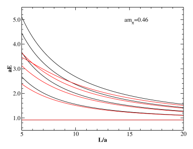
Figure 1: The total energy $E$ for four different levels in the continuum (black lines) and in the lattice (red lines) case versus $L$.

We will focus in the following on the case of a cubic lattice, characterised by a single side length $L$; it is valuable to remember that, in a cubic box if $n^{2}=\sum_{i=1}^{3}n_{i}^{2}$ is fixed, degenerate energy levels for different values of $n_{i}$ can appear. Sometimes we will refer to a specific level writing the three component vector as $(n_{x},n_{y},n_{z})$.

It is clear that the space-time discretization can have a strong effect in particular when the volume is small, i.e. large momentum, and $m_{\pi}$ is big. In Figure 1 we show a plot of the two formulas where it is evident that, for small volume ($L\lesssim 15$) and a mass $am_{\pi}=0.46$, the two spectra are very different; therefore we cannot use the continuum formula to describe our Monte Carlo results.

Note that in a general theory, such as QCD, where an expression like Eq. 2 is not available, we need to determine the non-zero-momentum single-particle energy levels numerically and then, to determine the two-particle energy spectrum, we simply multiply the results by a factor of two.

II.2 Avoided level crossing

Let us introduce another particle $\sigma$ in the box (at the moment, not interacting) with mass $m_{\sigma}$; we are interested in studying the elastic scattering between the $\pi$ particles, therefore we impose the constraint $2m_{\pi}<m_{\sigma}<4m_{\pi}$. In Figure 2 (Top) the $\sigma$ energy level is the horizontal line that intersects the two-particle levels at various system sizes $L$.

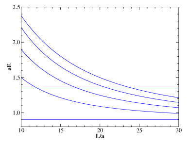
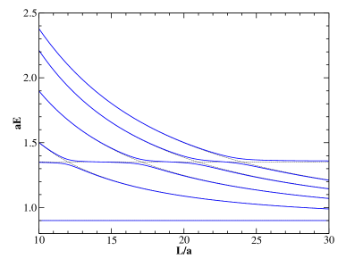
Figure 2: (Top) The spectrum of a system of two non-interacting particles of mass $am_{\pi}=0.4544$ worked out using Eq. 2; the horizontal line describes the particle $\sigma$ at rest with mass $am_{\sigma}=1.3517$. With these parameters the intersection between $\sigma$ and the two-particle level $n^{2}=1$, i.e. $(1,0,0)$, is set at $L=12$. (Bottom) Avoided level crossings where on the (Top) there were intersections between $\sigma$ and $2\pi$.

In Minkowski space if we introduce a three point interaction $\sigma\pi\pi$ between the fields, the $\sigma$ will become an unstable particle, a resonance, and decay into two $\pi$ particles. In Euclidean space and in a finite volume the scenario is different. First of all, the finite volume will prevent the $\sigma$ from being a resonance. This can be seen from two complimentary points of view. First of all, resonances appear as poles on the second Riemann sheet of the S-matrix. This second sheet is found by continuing through the multiparticle branch cut. However, in a finite volume the branch dissolves into a series of poles and hence this second Riemann sheet is lost, so the $\sigma$ may only appear as a pole on the physical sheet. Secondly, in a finite volume only certain discrete values of momenta are allowed. Conservation of momenta may require the two particles produced by the decay of the sigma to take on momenta outside these values, hence rendering the $\sigma$ stable. However because of the interaction, the energy eigenstates are a mixture of this stable $\sigma$ and the $2\pi$ Fock-states. One might attempt to avoid the fact that the $\sigma$ has become a stable state, by measuring on the lattice some appropriate $n$-point function which contains infinite-volume scattering information, such as the phase shift $\delta(p)$. However the Maiani-Testa theorem, Ref Maiani and Testa (1990), forbids this, as the Euclidean $n$-point functions lack the non-trivial complex phase which would directly characterise $\delta(p)$. Instead we turn to the effect that the mixing of the $\sigma$ has on the finite volume energy levels, which does contain information on its behaviour as a resonance in infinite volume: the most obvious feature is the avoided level crossings (ALCs), as shown in the lower panel of Figure 2.

II.2.1 ALC simple model

There is a very simple model that can be use both as a method to plot a spectrum where the ALCs are present but also as a model to test numerical methods for extracting the resonance parameters. The model is based on this correlation matrix:

$${\mathcal{C}}=\left(\begin{array}[]{ccc}m_{\sigma}&\lambda&\lambda\\ \lambda&E_{(0,0,0)}&0\\ \lambda&0&E_{(1,0,0)}\end{array}\right),$$ (3)

where $E_{(i,j,k)}$ are given by Eq. 2, here $i^{2}+j^{2}+k^{2}=n^{2}$. The diagonal terms correspond to the three lowest energy states of a theory where the $\sigma$ is stable and the off diagonal terms represent the interaction between the $\sigma$ and the two-particle states, of strength $\lambda$. To determine the spectrum associated to this matrix we have to diagonalize it; the eigenvalues of this matrix plotted as functions of $L$ give us the spectrum of an interacting toy theory. As an application we used it to plot Figure 2 (Bottom); the ALCs can be seen quite clearly.

II.3 Lüscher’s method

Probably the most well known method of obtaining information on resonances on the lattice is the method proposed by Lüscher in Ref Lüscher (1986, 1991a). The method works by using a mapping which converts information on the two-particle spectrum in the elastic region, in a finite volume, into information on the scattering phase shift in infinite volume. The scattering phase shift will then contain resonance parameters, for example near a resonance it will take the form

$$\delta(p)-\frac{\pi}{2}\approx\arctan\left(\frac{4p^{2}+4M_{\pi}^{2}-M_{\sigma}^{2}}{M_{\sigma}\Gamma_{\sigma}}\right)\ ,$$ (4)

and from this it is possible to extract the resonance mass and width. Note that, according to Eq. 4, the resonance appears when $\delta(p)=0$.

The energies of two-particle states are altered by a finite volume in two ways. First of all each individual particle in the pair has the virtual polarization coming from interactions “around the world”, discussed in Ref Lüscher (1986). However there is also a second effect resulting from their direct interaction with each other. It is this real interaction that Lüscher’s method exploits.

This effect is first derived in the case of non-relativistic quantum mechanics and then proven in the field theory case by relating it back to the non-relativistic one. In the quantum mechanical case, the finite volume Schrödinger equation, provided that the potential has finite range smaller than half the box volume, has two asymptotic forms. First, from a scattering theory perspective, since the potential has finite range, solutions will have the same asymptotic form as in infinite volume and hence will contain the scattering phase shift. Secondly, outside the potential, the Schrödinger equation reduces to the Helmholtz equation with eigenvalues given by the energy eigenvalues of the two-particle finite volume Hamiltonian. By matching these two asymptotic forms, a relationship between the two-particle energies in a finite volume and the scattering phase shift in infinite volume is obtained.

In quantum field theory one can decompose the four-point function into an infinite sum involving the Bethe-Salpeter Kernel and the two-point function. The four point function contains information on the two-particle energy spectrum and thus this expansion can be seen as an expansion for the two-particle energies. Analytic properties of the Bethe-Salpeter Kernel allow the contours of integration in this expansion to be shifted so that the two-point propagators take on a non-relativistic form. Once expressed this way, the expansion is no different from the Born expansion for a non-relativistic theory, with the Bethe-Salpeter Kernel filling the rôle of a potential. This Born expansion can be seen as coming from an effective Schrodinger equation for the two-particle wavefunction $\psi(r)$

$$-\frac{1}{2\mu}\nabla\psi(r)+\frac{1}{2}\int{d^{3}r^{{}^{\prime}}U_{W}(r,r^{{}^{\prime}})}\psi(r^{{}^{\prime}})=W\psi(r^{{}^{\prime}})\ .$$ (5)

The constant $W$ in Eq. 5 is the energy, when treated as non-relativistic problem, and it is related to the true physical energy in the Quantum Field Theory by $E=2\sqrt{m^{2}+mW}$. The same analytic properties mentioned above imply that the Bethe-Salpeter Kernel, as a potential, satisfies the conditions on a potential required for the quantum mechanical analysis. So the entire framework derived above for the non-relativistic case can simply be carried over to quantum field theory and Lüscher’s formula holds in this case as well.

This effective Schödinger equation is first constructed in Ref Lüscher (1986).

The relationship derived from this analysis is

$$\delta(p) =-\phi(\kappa)+\pi n\ ,$$ (6)

$$\tan(\phi(\kappa)) =\left(\frac{\pi^{3/2}\kappa}{Z_{00}(1;\kappa^{2})}\right),\quad\kappa=\frac{pL}{2\pi}\ ,$$ (7)

where $p$ is the relative momentum between the two decay particles. $\mathcal{Z}_{js}(1;q^{2})$ is a generalised Zeta function, given by

$$\mathcal{Z}_{js}(1;q^{2})=\sum_{\underline{n}\in\mathbb{Z}^{3}}\frac{r^{j}Y_{js}(\theta,\phi)}{(\underline{n}^{2}-q^{2})^{s}}\ ,$$ (8)

where $Y_{js}(\theta,\phi)$ are the spherical harmonics. Eq. 6 is known as Lüscher’s formula. It should be mentioned that Eq. 6 is in fact a special case of the more general expression derived in Ref Lüscher (1991a). The formula quoted here is for the spin-$0$ channel, which is the only one relevant here. Also in deriving the formula a change in the contour of integration allowed the propogators to be rewritten as nonrelativistic propogators. However if the volume is quite small this cannot be done because the two-point functions will not have the correct initial form due to the polarization from around the world as mentioned earlier. For this reason one must check that these virtual polarisation effects become negligable in order to use Lüscher’s formula.

To obtain resonance parameters using this relationship one proceeds as follows:

1. Using the Monte Carlo data, obtain the two-particle energy spectrum $E_{n}(L)$ as a function of the volume;

2. Using dispersion relations, obtain a momentum from the energy spectrum, $p_{n}(L)$;

3. Compute the appropriate values of $\phi(\kappa)$. Eq. 6 will then map the values $p_{n}(L)$ to values of $\delta(p_{n}(L))$;

4. If this procedure is repated for several energy levels and volumes, a profile of $\delta(p)$ is produced;

5. This profile can then be fitted against the Breit-Wigner form for $\delta(p)$ in the vicinity of a resonance as given in Eq. 4. This fit should give the resonance mass $M_{\sigma}$ and width $\Gamma_{\sigma}$.

II.4 Histogram method

An alternative method of determining the parameters of a resonance is based on a different way of analyzing the finite volume energy spectrum, Ref Bernard et al. (2008). The basic idea is to construct a probability distribution $W(E)$ according to the prescriptions:

1. Measure the two-particle spectrum $E_{n}(L)$ for different values of $L$ and for $n=1,\cdots,N$ levels;

2. Interpolate the data with fixed $n$ in order to have a continuous function $E_{n}(L)$ in an entire range $L\in[L_{0},L_{M}]$;

3. Slice the interval $[L_{0},L_{M}]$ into $M$ equal parts with length $\Delta{L}=(L_{M}-L_{0})/M$;

4. Determine $E_{n}(L_{i})$ for each $L_{i}$ ($i=0,\cdots,M$);

5. Choose a suitable energy interval $[E_{min},E_{max}]$ and introduce an equal-size energy bin with length $\Delta{E}$;

6. Count how many eigenvalues $E_{n}(L_{i})$ are contained in each bin;

7. Normalize this distribution in the interval $[E_{min},E_{max}]$.

The distribution considered in Ref Bernard et al. (2008) is $W(p)$ but this does not have an important effect on our analysis; as a matter of fact, the relation between them is (it is based on the definition given in Eq. 10):

$$W(p)=W(E)\left(\frac{\partial{E}}{\partial{p}}\right)\ ,$$ (9)

where the correct dispersion relation we should use is Eq. 2; the multiplicative term will not modify the Breit-Wigner shape near the resonance.

It is possible to show that the probability distribution $W(p)$ is given by

$$W(p)=c\sum_{n=1}^{N}\left[p^{\prime}_{n}(L)\right]^{-1}$$ (10)

and differentiating the Lüscher formula with respect to $L$, it turns out ($c$ is a normalization constant):

$$W(p)=\frac{c}{p}\sum_{n=1}^{N}\left[L_{n}(p)+\frac{2\pi\delta^{\prime}(p)}{\phi^{\prime}(q_{n}(p))}\right]\ .$$ (11)

If one expands $L_{n}(p)$ around the case of $\delta=0$, when the there is no interaction between the $\sigma$ and the two-particle states, this takes the form:

$$C^{-1}W(p)= \sum_{n=1}^{N}\frac{2\pi}{p^{2}}\overline{\kappa}_{n}-$$ (12)

$$\sum_{n=1}^{N}\frac{2\pi}{p}\frac{1}{\phi^{{}^{\prime}}(\overline{\kappa}_{n})}\left(\frac{\delta(p)}{p}-\delta^{{}^{\prime}}(p)\right)+\mathcal{O}(\delta^{2})\ .$$ (13)

The first term is equivalent to the histogram that would be constructed in a theory where the $\sigma$ is a stable particle. We will call this histogram the free background, $C_{0}^{-1}W_{0}(p)$, where $C_{0}$ is its normalisation constant. If we subtract it from the interacting histogram we obtain

$$C^{-1}W(p)-C_{0}^{-1}W_{0}(p)=$$ (14)

$$-\sum_{n=1}^{N}\frac{2\pi}{p}\frac{1}{\phi^{{}^{\prime}}(\overline{\kappa}_{n})}\left(\frac{\delta(p)}{p}-\delta^{{}^{\prime}}(p)\right)+\mathcal{O}(\delta^{2})\ .$$ (15)

In the limit of an infinite number of energy levels, i.e. infinite volume, the terms of $\mathcal{O}(\delta^{2})$ are very small for the vast majority of energy levels and so become negligable. Hence we obtain:

$$C^{-1}W(p)-C_{0}^{-1}W_{0}(p)\approx$$ (16)

$$-\left[\sum_{n=1}^{N}\frac{2\pi}{\phi^{{}^{\prime}}(\overline{\kappa}_{n})}\right]\frac{1}{p}\left(\frac{\delta(p)}{p}-\delta^{{}^{\prime}}(p)\right)\ .$$ (17)

However we can see that

$$\sum_{n=1}^{N}\frac{2\pi}{\phi^{{}^{\prime}}(\overline{\kappa}_{n})}$$ (18)

is just a constant independent of $\delta$ or $p$ and so it can just be absorbed into the normalisation constant of the histogram to give us:

$$W(p)-W_{0}(p)\propto\frac{1}{p}\left(\frac{\delta(p)}{p}-\delta^{\prime}(p)\right)\ .$$ (19)

This last quantity is determined by $\delta(p)$ alone and close to the resonance, assuming a smooth dependence on $p$ for the other quantities, it follows the Breit-Wigner shape of the scattering cross section with the same parameters:

$$W(p)-W_{0}(p)\propto\frac{1}{[E(p)^{2}-M_{\sigma}^{2}]^{2}+M_{\sigma}^{2}\ \Gamma^{2}}\ .$$ (20)

To emphasize the approximations that are present we note that, because

$$\delta(p)=\arctan\left(\frac{M_{\sigma}\Gamma}{M_{\sigma}^{2}-E^{2}(p)}\right)\ ,$$ (21)

then we can work out:

$$\delta^{\prime}(p)=\frac{8M_{\sigma}\Gamma p}{[M_{\sigma}^{2}-E^{2}(p)]^{2}+M_{\sigma}^{2}\Gamma^{2}}\ ;$$ (22)

therefore we can see that the Breit-Wigner shape of Eq. 20 is entirely due to $\delta^{\prime}(p)$. It should also be noted that this Histogram method does no require one to have knowledge of the function $\phi(\kappa)$, unlike like Lüscher’s method.

In Ref Bernard et al. (2008) this method is tested on synthetic data produced using the Lüscher formula by experimentally measured phase shifts and in Ref Morningstar (2008) it is tested on nonrelativistic quantum mechanics. The main task of our work is to test this method on an effective field theory where a resonance emerges, producing data by lattice simulations.

III The $O(4)$ sigma model

The model we have used in our simulations is the $O(4)$ model in the broken phase. This model has previously been used to test Lüscher’s method, Ref Gockeler et al. (1994). The Lagrangian is the following (with $i=1,2,3,4$):

$$\mathcal{L}=\frac{1}{2}\partial\phi_{i}\partial\phi_{i}+\lambda(\phi_{i}^{2}-\nu^{2})^{2}-m^{2}_{\pi,0}\nu\phi_{4}\ .$$ (23)

The term proportional to $\phi_{4}$ is introduced to break the symmetry explicitly in order to give mass to the three Goldstone bosons. To understand the meaning of the terms and the parameters in the Lagrangian, we first introduce the new fields $\sigma$ and $\rho_{i}$ (with the constraint $\rho_{i}\rho_{i}=1$):

$$\phi_{i}=(\nu+\sigma)\rho_{i}\ ,\qquad\mbox{with $i=1,2,3,4$}\ ;$$ (24)

then, we expand the potential around the classical minimum $\phi_{i}\phi_{i}=\nu^{2}$ (using also $\rho_{i}\partial\rho_{i}=0$):

$$\mathcal{L}=\frac{1}{2}\nu^{2}\partial\rho_{i}\partial\rho_{i}+\frac{1}{2}\sigma^{2}\partial\rho_{i}\partial\rho_{i}+$$

$$\frac{1}{2}\partial\sigma\partial\sigma+\nu\sigma\partial\rho_{i}\partial\rho_{i}+\lambda\sigma^{4}+4\nu^{2}\lambda\sigma^{2}+$$

$$4\nu\lambda\sigma^{3}-m_{\pi,0}^{2}\nu^{2}\rho_{4}-m_{\pi,0}^{2}\nu\sigma\rho_{4}\ .$$ (25)

The $\sigma$ field is clearly related to the massive $\phi_{4}$ field in the original Lagrangian, whereas the four constrained fields $\rho_{i}$ are related to the three “pions”. In the form Eq. 25 we can not directly interpret the physical content of the Lagrangian, due to the presence of linear terms. Particularly it is not obvious that the explicit breaking term has given the three Goldstone bosons a mass.

There is an easy way to rewrite the Langrangian to make all of this more obvious, based on the treatment of the non-linear sigma model (see for example Ref DeGrand and Detar (2006), Sec 2.4.3.).

We introduce the pions using an element of $SU(2)$:

$$U=e^{\frac{i}{\nu}\pi_{j}\sigma_{j}}=\cos{\left(\frac{|\vec{\pi}|}{\nu}\right)}+i\sigma_{j}\frac{\pi_{j}}{|\vec{\pi}|}\sin{\left(\frac{|\vec{\pi}|}{\nu}\right)}\ ,$$ (26)

where $\sigma_{j}$ are the three Pauli matrices and where $\nu$ plays the rôle of the pion decay constant. On the other hand, we can also form $SU(2)$-valued fields from our $\rho$-fields by

$$U=\rho_{4}+i\sigma_{j}\rho_{j}\ ,$$ (27)

with $j=1,2,3$ and the constraint $\rho_{4}^{2}+\rho_{j}\rho_{j}=1$. We can therefore identify the connection between the three fields $\pi_{j}$ and the fourth $\rho_{j}$, using Eq. 26 and Eq. 27:

$$\rho_{4} = \cos{\left(\frac{|\vec{\pi}|}{\nu}\right)}\ ,$$ (28)

$${\rho}_{j} = \frac{\pi_{j}}{|\vec{\pi}|}\sin{\left(\frac{|\vec{\pi}|}{\nu}\right)}\ .$$ (29)

We can now replace the $\rho$ fields in the Langrangian using the expression $\frac{1}{2}\operatorname{Tr}(\partial_{\mu}U\partial_{\mu}U^{\dagger})$. For the $\rho$ fields this is

$$\frac{1}{2}\operatorname{Tr}(\partial_{\mu}U\partial_{\mu}U^{\dagger})=\sum_{i=1}^{4}\partial_{\mu}\rho_{i}\partial_{\mu}\rho_{i}\ .$$ (30)

For the pion fields this gives

$$\frac{1}{2}\operatorname{Tr}(\partial_{\mu}U\partial_{\mu}U^{\dagger})=\frac{1}{\nu^{2}}\sum_{i=1}^{3}\partial_{\mu}\pi_{i}\partial_{\mu}\pi_{i}\ ,$$ (31)

and so we have:

$$\sum_{i=1}^{4}\partial_{\mu}\rho_{i}\partial_{\mu}\rho_{i}=\frac{1}{\nu^{2}}\sum_{i=1}^{3}\partial_{\mu}\pi_{i}\partial_{\mu}\pi_{i}\ .$$ (32)

Eq. 28 and Eq. 32 can then be substituted into the original Lagrangian, Eq. 25. Expanding the $\cos\left(\frac{|\vec{\pi}|}{\nu}\right)$, which has replaced the $\rho_{4}$ field, we obtain as our Lagrangian:

$$\mathcal{L}=\frac{1}{2}\partial_{\mu}\pi_{j}\partial_{\mu}\pi_{j}+\frac{1}{2\nu^{2}}\sigma^{2}\partial_{\mu}\pi_{j}\partial_{\mu}\pi_{j}+\frac{1}{2}\partial_{\mu}\sigma\partial_{\mu}\sigma+$$

$$\frac{1}{\nu}\sigma\partial_{\mu}\pi_{j}\partial_{\mu}\pi_{j}+\lambda\sigma^{4}+4\nu^{2}\lambda\sigma^{2}+4\nu\lambda\sigma^{3}+$$

$$\frac{1}{2}m_{\pi,0}^{2}\pi_{j}\pi_{j}+\frac{m_{\pi,0}^{2}}{2\nu}\sigma\pi_{j}\pi_{j}\ +\ldots\ ,\quad$$ (33)

where the higher order terms include higher order couplings between the pions and the $\sigma$ resonance, as well as pion self-interaction terms. We can see that the $\sigma$ field gets a bare mass

$$m_{\sigma}=2\nu\sqrt{2\lambda}\ ,$$ (34)

and due to terms such as the three-point interaction $\nu\sigma\partial\rho_{i}\partial\rho_{i}$ the sigma particle is unstable. We can also see that the parameter $m_{\pi,0}$, that we introduced in Eq. 23, functions as the bare pion mass. So our explicit soft-breaking term has given the Goldstone bosons a mass.

Two things should be noted about the three-point interaction term. First of all, it depends on $\nu$, so the sigma resonance should be broader with decreasing values of $\nu$. We will not however make direct use of this, since making $\nu$ too small leads to symmetry restoration. The interaction also contains a derivative. In momentum space this will give an extra $p^{2}$ term to the vertex appearing in Feynman diagrams. We expect the interaction between the pions and the sigma resonance to be stronger when the pions have larger relative momentum. The decay rate of the sigma resonance will also depend on $\lambda$, since the $\sigma$ field self-coupling terms will affect the interactions between the $\sigma$-particle and the pions.

For certain values of the parameters the $O(4)$ symmetry will be restored and the theory will enter the unbroken phase. Since we do not want this to occur we must avoid the region of the $\lambda$, $\nu$ parameter space in which the symmetry remains unbroken. For any fixed value of $\lambda$ the symmetry is restored when $\nu$ is sufficiently small. The point of this phase transition $\nu_{*}(\lambda)$ increases with increasing $\lambda$. In particular

$$\lim_{\lambda\rightarrow\infty}\nu_{*}(\lambda)\approx 0.78\ .$$ (35)

Hence we will always keep $\nu$ above $0.78$, specifically we use $\nu=1$ or $1.05$, to guarantee that the symmetry remains broken.

A derivation of Eq. 35 is contained in Ref Gockeler et al. (1994), although there, due to different parameters being used, it appears as $\kappa_{c}\approx 0.304$.

IV Monte Carlo simulation

The theory described by the Lagrangian in Eq. 23, was simulated using an over-relaxation algorithm for the first three near-Goldstone fields, followed by a Metropolis update to guarantee the ergodicity, and a Metropolis algorithm for the massive field, $\phi_{4}$.

In order to determine the single particle spectrum we first introduce the partial Fourier transform (PFT) of the four fields $\phi_{i}$:

$$\tilde{\phi_{i}}(\vec{n},t)=\frac{1}{V}\sum_{x}\phi_{i}(\vec{x},t)e^{-i\vec{x}\vec{p}}\ ,\qquad p_{i}=\frac{2\pi}{L_{i}}n_{i}\ ,$$ (36)

where $n_{i}=0,\ldots,L_{i}-1$. The single particle mass is extracted from the zero momentum correlation function ($\vec{n}=\vec{0}$):

$$C_{i}(t)=\langle\tilde{\phi_{i}}(\vec{n},t)\tilde{\phi_{i}}(-\vec{n},0)\rangle\ .$$ (37)

In particular with $i=1,2,3$ we can determine the mass of the three pion fields; with $i=4$ we extract the mass of the $\sigma$ particle. In Monte Carlo simulation, the mass of the lightest state is usually determined with better statistical precision, and this is observed here, where $m_{\pi}$ is determined with a higher precision then $m_{\sigma}$; this is not a problem because we are mainly interested in a good resolution of states consisting of two pions and these energies are well determined.

The two-particle spectrum is measured by introducing operators with zero total momentum and zero isospin:

$$O_{\vec{n}}(t)=\sum_{i=1}^{3}\tilde{\phi_{i}}(\vec{n},t)\tilde{\phi_{i}}(-\vec{n},t)\ ;$$ (38)

we take into account $N-1$ different operators corresponding to $n^{2}=0,1,\ldots,N-2$. An $N$-th operator, that clearly has the correct quantum number is the PFT of the field $\sigma$ (actually of $\phi_{4}$) with $\vec{p}=0$.

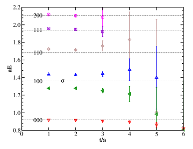
Figure 3: Effective mass versus time as determined by the diagonalization of the correlation matrix $C_{ij}$. The dashed constant lines describe the free two-particle spectrum. Simulation parameters: $\nu=1.0$, $\lambda=1.4$, $am_{\pi}=0.36$, volume=$12^{3}\times 64$.

To determine the energy levels we use a method, introduced in Ref Michael (1985) (see also Ref Lüscher and Wolff (1990)), based on a generalized eigenvalue problem applied to the correlation matrix function $C_{ij}(t)=\langle O_{i}O_{j}\rangle$, that is a matrix whose elements are all possible correlators between the $N$ operators:

$$C(t)\psi=\lambda(t,t_{*})C(t_{*})\psi\ ,$$ (39)

where $t_{*}$ is fixed to a small value (we verified that in this model the results are insensitive to its value, so we chose $t_{*}=0$). It is possible to show that the eigenvalues, for $\alpha=1,\ldots,N$, behave as

$$\lambda_{\alpha}(t,t_{*})=e^{-(t-t_{*})E_{\alpha}}\ ,$$ (40)

where $E_{\alpha}$ describes the spectrum of the theory; a typical result is shown in Figure 3. Using this method we can see a wide plateau of approximately six lattice spacings for the ground-state, dominated by two pions at rest that starts from $t_{0}=1$ in this case. The width of the plateau decreases with increasing energy and it is just 2 lattice spacing for the level $(2,0,0)$ the onset of the plateau also occurs later. In Fig. 3, it is evident there is strong mixing between the state resembling two pions, each with momentum $n=\pm(1,0,0)$ and the $\sigma$ state, illustrating an example avoided level crossing.

IV.1 Histogram Results

In order to test the applicability of the two methods for different widths of resonance, we consider three different sets of parameters in the lagrangian. In all three simulations, the time extent of the lattice is fixed to $L=64a$. The first simulation is performed using $\nu=1.0$, $\lambda=1.4$, $am_{\pi,0}=0.36$. These parameters were determined to have the intersection between the $\sigma$ energy level and $n=(1,0,0)$ two-particle energy level in the absence of interaction at around $L=12a$. The measured mass for the pion turns out to be $am_{\pi}=0.460(2)$. The first six energy levels were determined clearly for different volumes in the range $8\leq L/a\leq 19$. The fractional error on the measured energies was in the range 0.5% - 1.0%. The top panel of Figure 4 shows the results of this set of simulations. Each energy was determined from statistical fitting, choosing the onset of the plateau to be $t_{0}=2$.

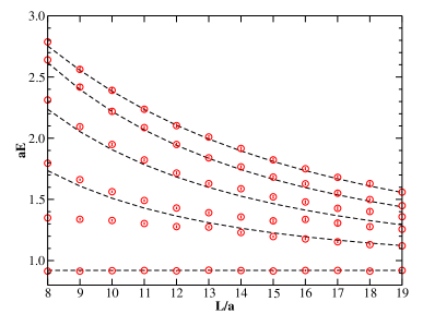
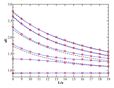
Figure 4: (Top) Spectrum of the theory for different values of the volume for the following simulation parameters: $\nu=1.0$, $\lambda=1.4$, $am_{\pi,0}=0.36$. The dashed lines describe the free two-particle spectrum. (Bottom) The interpolated data using a polynomial.

Constructing a histogram where a resonance is clearly seen requires a large set of lattice volumes and energy levels. We found the stability of the histogram could be enhanced by interpolating the spectrum data using polynomials in $L$ over all values of $L/a$ in the measured range and using these polynomials to generate more data for the histogram. The lower panel of Fig. 4 shows the resulting polynomial fit. Polynomials of order 3, 4 and 5 were used, which provided a means of evaluating the systematic errors in the final results. The dashed lines in Fig. 4 show the free two-particle spectrum, calculated using Eq. 2.

In order to control the dominant distortions in the free spectra arising simply from discretisation artefacts for these high-lying states, the energy curves for the non-interacting pions were computed using the free dispersion relation after first computing the subtracted mass $m_{\pi,r}$ using the rest-energy of a single pion $m_{\pi}$:

$$m_{\pi}=4\sinh^{-1}\left[{\frac{1}{2}m_{\pi,r}}\right]\ .$$ (41)

These curves show very good agreement with the observed spectra away from the resonance even at very high energies. The pion mass measured in these simulations is $am_{\pi}=0.460(2)$, which differs from the parameter in the lattice lagrangian $am_{\pi,0}=0.36$ due to renormalisation effects of the interacting theory.

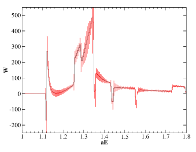
Figure 5: The probability distribution $\tilde{W}=W-W_{0}$ obtained from data from Figure 4.

This free spectrum is used to determine the distribution $W_{0}(p)$ which is then subtracted from $W$, obtained from the interacting spectrum. It is important to note that if $N$ levels are used to plot $W$ in the interacting spectrum, then the number of levels needed from the free spectrum to determine $W_{0}$ is $N-1$. This takes into account the extra level arising from the resonance and ensures the correct modes are subtracted at the upper and lower ends of the energy range. Note that, in the general case, if the same number $N$ of levels are used the final result will be affected by the presence of unwanted peaks which potentially could hidden the presence of the resonance.

Using polynomials, we are able to produce a large number of data at arbitrary values of $L/a$; we use a resolution of $a\Delta{L}=0.001$. Using a bin width of $a\Delta{E}=0.005$, we get the probability distribution $W$, described in Sec II.4, and, consequently, the histogram $\tilde{W}=W-W_{0}$ of Figure 5. Note that to get $\tilde{W}$ both $W$ and $W_{0}$ are determined from the same range of $L/a\in[8,19]$. The error bars in Figure 5 then include both the systematic (determined by the different results we get using the different polynomials) and statistical errors coming from the histogram $W$ and the statistical errors coming from the determination of $W_{0}$ including the statistical error propagating from $m_{\pi}$ via Eq. 2.

Clearly, the shape of the histogram in Figure 5 is far from a Breit-Wigner distribution. The dominant reason for the distortions is that our Monte Carlo measurement determined only six energy levels while the conclusions of Sec II.4 are true only in the limit of an infinite number of levels. Many jumps and spikes are seen. Our task is now to try to modify the analysis in order to get fewer artefacts from the same raw data. We investigated the origin of the spikes and concluded that they are related to subtractions of an “incorrect” background $W_{0}$. It is easy to see that the spikes appear every time there is the intersection between the six levels of the interacting spectrum or of the five levels of the free spectrum with the extremities of the volume range at $L/a=8$ and $L/a=19$. Near those two extremities a more careful modelling of the free background is needed;

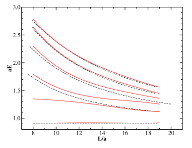
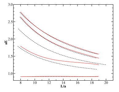
Figure 6: (Top) Energy levels of Figure 4 (Bottom) with the correct free two-particle spectrum background. (Bottom) Energy levels where we deleted the two levels that appear without their own background.

Figure 6 (Top) shows a corrected background subtraction. In order to correctly subtract the free background, each free spectrum line is extended using the polynomial fitting form. This is done so that the extremity of each line has energy equal to the value at the end of the interacting spectrum line closest to it. In this way all interacting lines are subtracted correctly rather than the subtraction being affected by the limit of the volume range that we are actually using in our simulations. Using this procedure to determine $W_{0}$ we get the correct histogram of Figure 7 (Top).

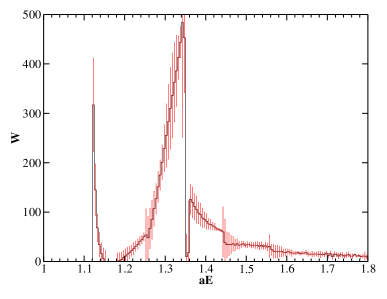
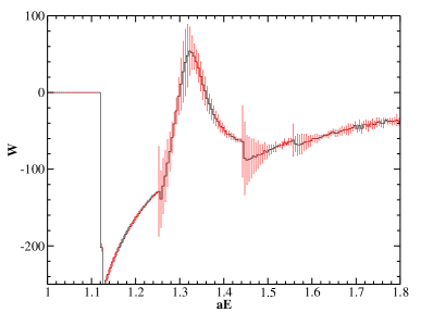
Figure 7: (Top) Probability distribution $\tilde{W}$ obtained by data from Figure 6 (Top). (Bottom) Probability distribution $\tilde{W}$ obtained from Figure 6 (Bottom).

Unfortunately, in Figure 7 (Top), we continue to see a discontinuity at $aE\approx 1.35$; the origin of this can be understood by looking at Figure 6 (Top). There are two extremity lines, one at $L=8a$ and one at $L=19a$ which are both around $E\approx 1.35$, that occur without a corresponding “background”; actually, in this case the background is the resonance itself we are looking for.

Therefore, there is no way to avoid the presence of this jump because we do not know anything about the resonance; the only thing we can do is to completely exclude from our analysis those two levels, Figure 6 (Bottom), hoping that the resonance still appears in other modes. In Figure 7 (Bottom) we show the probability distribution $\tilde{W}$ in this last case; now clearly a Breit-Wigner distribution emerges.

It is now possible to fit these data to Eq. 20 to determine the parameters of the resonance, Figure 8. Applying a sliding window procedure around the peak gives: $aM_{\sigma}=1.330(5)$ and $a\Gamma_{\sigma}=0.10(5)$.

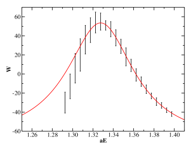
Figure 8: Data from Figure 7 (Bottom) that we fitted to determine the resonance parameters with the final curve fitting.

We simulated the theory at a second set of parameters corresponding to a broader resonance: $\nu=1.0$, $\lambda=4.0$, $am_{\pi,0}=0.56$. In this case, the parameters were chosen such that the intersection occurs between the $\sigma$ energy level and $n=(1,0,0)$ two-particle energy level close to $L=8a$. The measured mass for the pion turns out to be $am_{\pi}=0.657(3)$. In Figure 9 (Top) we plot the spectrum for $6\leq L/a\leq 20$ for the first six levels; in this case the onset value for the plateaux is $t_{0}=1$ and the relative error varies in the range 0.05% - 0.2%.

We repeat the procedure described above. Taking care of the correct subtraction of the background we get the histogram of Figure 9 (Bottom). Clearly we see two discontinuities, related to the two levels in the interacting theory that appear without a corresponding background: one at $E\approx 1.95$ is due to the intersection at $L=6a$ and the other one at $E\approx 2.00$ which is due to the intersection at $L=20a$.

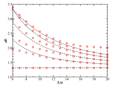
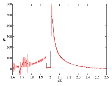
Figure 9: (Top) Spectrum of the theory for different values of the volume for the following simulation parameters: $\nu=1.0$, $\lambda=4.0$, $am_{\pi,0}=0.56$. (Bottom) The probability distribution considering the correct background.

When we exclude the two levels which have no corresponding background signal, we get the histogram of Figure 10 (Top). In this case again we can clearly see a Breit-Wigner shape and we can fit these data, as shown in Figure 10 (Bottom), obtaining the following parameters: $aM_{\sigma}=2.01(2)$, $a\Gamma_{\sigma}=0.35(10)$.

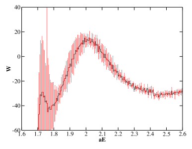
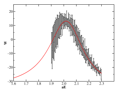
Figure 10: (Top) Probability distribution $\tilde{W}$ using the correct background and excluding the two levels that are without a corresponding background. (Bottom) Data we fitted to determine the resonance parameters with the final curve fitting. Simulation parameters: $\nu=1.0$, $\lambda=4.0$, $am_{\pi,0}=0.56$.

Finally, a third series of simulations was performed with parameters $\nu=1.0$, $\lambda=200.0$, $am_{\pi,0}=0.86$. They have been tuned to have the intersection between the $\sigma$ energy level and $(2,0,0)$ two-particle energy level around $L=10a$. Because in this case we are considering pions with higher momentum, we expect the width of the resonance to be larger than the previous cases, for reasons discussed at the end of Sec III. For this analysis, we take into account 13 levels to describe the shape of the resonance better. In Figure 11 the spectrum for $6\leq L/a\leq 15$ is plotted. The onset value for the plateaux is $t_{0}=1$ and the relative error varies in the range 0.15% - 0.4%. The measured mass for the pion is $am_{\pi}=0.938(3)$.

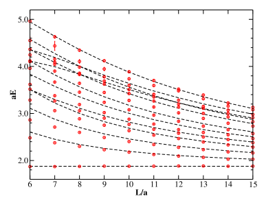
Figure 11: Spectrum of the theory with simulation parameters: $\nu=1.0$, $\lambda=200.0$, $am_{\pi,0}=0.86$.

In Figure 12 (Top) as in the previous cases we show the probability distribution taking in account all levels. We can see that a possible peak is present around a value of the mass $am\approx 2.8$. Unfortunately, as seen in Figure 12 (Bottom), when we exclude the two levels the probability distribution plot is flat and no Breit-Wigner shape emerges. It is clear that in this case, the only way to determine the parameters of the resonance is to considerably increase the number of measurements and consequently to decrease the relative errors in the spectrum determination.

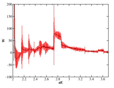
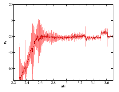
Figure 12: (Top) The probability distribution considering the correct background. (Bottom) Probability distribution $\tilde{W}$ using the correct background and excluding the two levels that are without a corresponding background. Simulation parameters: $\nu=1.0$, $\lambda=200.0$, $am_{\pi,0}=0.86$.

IV.2 Lüscher’s method results

As outlined in Sec II.3, Lüscher’s method provides a way to relate information on the two-particle spectrum in the elastic region to the scattering phase shift. As the scattering phase shift depends on momentum the first step is to convert the energy spectra data into momentum spectra data.

The relation between the energy and the momentum is given by the dispersion relations; however there is the choice of using the lattice dispersion relations or the continuum dispersion relations. Naturally the lattice dispersion relations are seen to better represent the data, but it is interesting to observe what occurs when the continuum dispersion relations are used.

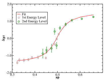
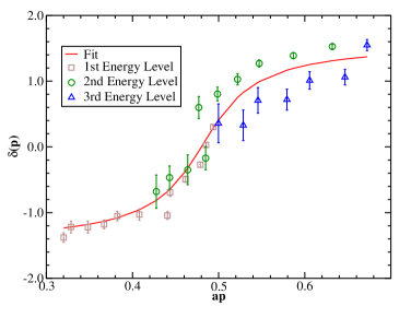
Figure 13: (Top) $\delta(p)$ using Lattice dispersion relations at: $\nu=1.0$, $\lambda=1.4$, $am_{\pi,0}=0.36$. (Bottom) Same parameters, but with continuum dispersion relations. Both done with our $\phi(\kappa)$ approximation.

When the momenta spectrum $p_{n}(L)$ has been obtained through the dispersion relations it is necessary to have some knowledge of the function $\phi(\kappa)$ appearing in Eq. 6 in order to translate to the scattering phase shift $\delta(p)$. In some works, $\phi(\kappa)\approx\pi\kappa^{2}$ is taken as a good approximation, but it is possible that for low values of $\kappa$ this will not be sufficiently accurate. For more accurate results one should numerically evaluate $\phi(\kappa)$. In essence this amounts to a numerical evaluation of $\mathcal{Z}_{00}(r;q^{2})$. However, in the expression Eq. 8 for $\mathcal{Z}_{00}(r;q^{2})$ the value of $r=1$, used in the application of Lüscher’s method, is outside the domain of convergence.

Fortunately there is an integral representation of $\mathcal{Z}_{00}(1;q^{2})$ (Appendix C of Ref Lüscher (1991b)) which analytically continues to the point $r=1$. The expression is also amenable to numerical evaluation. Using the values obtained from this evaluation of $\mathcal{Z}_{00}(1;q^{2})$, we performed a fit of $\phi(\kappa)$ to obtain as our approximation in the range $\kappa\in\left[0.1,1.5\right]$

$$\phi(\kappa)\approx(-0.09937)\kappa^{8}+(0.47809)\kappa^{6}+$$

$$(-0.62064)\kappa^{4}+(3.38974)\kappa^{2}\ .$$ (42)

Note that it can be shown from its definition that $\phi(\kappa)$ has a Taylor expansion consisting of only even powers of $\kappa$. The error of using this approximation in place of the true values, within the given range, is significantly less than other errors and can be neglected at later stages of the analysis. This approximation is used here simply to demonstrate the deviation of the function from $\phi(\kappa)\approx\pi\kappa^{2}$ and how this can affect the results.
We can now use Eq. 6 to map our energy spectrum data to $\delta(p)$. The choice of dispersion relations and approximation of $\phi(\kappa)$ could possibly change the results significantly so all four choices are considered.

		$\phi(\kappa)$		$\pi\kappa^{2}$
$\nu$	$\lambda$	$aM_{\sigma}$	$a\Gamma_{\sigma}$	$aM_{\sigma}$	$a\Gamma_{\sigma}$
1.0	1.4	1.32(8)	0.117(9)	1.4(1)	0.16(5)
1.0	4	2.1(4)	0.39(4)	2.2(4)	0.42(5)
1.0	200	3(1)	1.2(7)	3(1)	2(2)

Table 1: Resonance mass and decay width using two different approximations for $\phi(\kappa)$, with continuum dispersion relations.

Firstly, for the choice of dispersion relations, Figure 13 shows that the lattice relation brings the energy levels close to a single arctangent profile whereas the continuum relations give a much more scatter. Also notice that the third energy level is not mapped to the elastic region with the lattice dispersion relations. The lattice dispersion relations also have smaller errors.

		$\phi(\kappa)\quad$		$\pi\kappa^{2}$
$\nu$	$\lambda$	$aM_{\sigma}$	$a\Gamma_{\sigma}$	$aM_{\sigma}$	$a\Gamma_{\sigma}$
1.0	1.4	1.35(2)	0.115(8)	1.36(4)	0.17(2)
1.0	4	2.03(2)	0.35(2)	2.2(2)	0.42(5)
1.0	200	3.1(7)	1.2(5)	3(1)	2(1)

Table 2: Resonance mass and decay width determinations using two different approximations for $\phi(\kappa)$ and lattice free dispersion relations.

After fitting, the results for the resonance mass and decay width in the two approximations using continuum dispersion relations are shown in Table 1 and the lattice dispersion relations in Table 2.

The choice of approximation for $\phi(\kappa)$ can be seen to most strongly affect the errors and values of the decay width. A possible reason for this is that different approximations of $\phi(\kappa)$ will change the slope of the scattering phase shift, which is directly related to the the decay width of the resonance. So it would appear that the lattice dispersion relations should be used for a clear arctangent profile and a good approximation to $\phi(\kappa)$, such as Eq. 42, so that the slope remains undistorted to give accurate information on the decay width.

It can be seen that the errors increase as the resonance gets broader. Similar to the histogram method this is related to the distinctive profile of the resonance being washed out. In the histogram method the distinctive Breit-Wigner form flattened out into a flat profile, here the typical arctangent profile of the phase shift becomes a straight line. In this case the resonance width can be changed within a wide margin without affecting the profile of the phase shift, hence the greater errors. Figure 14 shows a comparsion between the broadest case and the narrowest case.

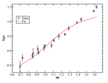
Figure 14: Phase shift for narrow ($\nu=1.0$, $\lambda=1.4$, $am_{\pi,0}=0.36$) and broad ($\nu=1.0$, $\lambda=200.0$, $am_{\pi,0}=0.86$) resonances.

IV.3 Comparison

Results from a comparison between Lüscher’s method and the histogram method are shown in Table 3.

		Lüscher		histogram
$\nu$	$\lambda$	$aM_{\sigma}$	$a\Gamma_{\sigma}$	$aM_{\sigma}$	$a\Gamma_{\sigma}$
1.0	1.4	1.35(2)	0.115(8)	1.33(5)	0.10(5)
1.0	4	2.03(2)	0.35(2)	2.01(2)	0.35(10)
1.0	200	3.1(7)	1.2(5)	—	—

Table 3: A comparison between the Lüscher and the histogram method. For the very broad resonance, no determination of the resonance parameters was obtained.

Lüscher’s method gives smaller errors than the histogram method, but the results are broadly consistent. Lüscher’s method manages to provide some estimate on the width of the resonance in the broad case. The broad resonance becomes a problem for the histogram method because there is no obvious peak to indicate the resonance mass and hence no width of that peak to determine the decay width. One would need very precise data in order to avoid a washing out of the structure of the histogram. Lüscher’s method also becomes more difficult to apply in the case of broad resonances. Here, the profile of $\delta(p)$ is quite flat, hence a large range of parameters will be capable of fitting to the profile. Again an accurate determination of the energy levels is required to determine the profile precisely enough so that this is prevented. Considering the amount of work necessary until one can use the histogram method (as detailed above), Lüscher’s method is considerably easier to apply, provided one has a good approximation of $\phi(\kappa)$. However, the histogram method can be used as a visual tool for spotting the resonance.

One restriction of Lüscher’s formula is that it only applies in the elastic region. It is possible that the histogram method will provide a means of determining the presence of a resonance in the inelastic region. Certainly, a histogram can be constructed in the inelastic region; the only difficulty is that with the inapplicability of Lüscher’s formula it is unclear that the parameters of this histogram will have any relation to those of the resonance.

IV.4 Inelastic scattering

We want to discuss now what happens when we tune the resonance parameters to have a mass resonance greater then four times the pion mass, i.e. greater then the elastic threshold.

We run a series of simulations with parameters $\nu=1.05$, $\lambda=0.85$, $am_{\pi,0}=0.17$. They have been tuned to have the intersection between the $\sigma$ energy level and $(1,0,0)$ two-particle energy level around $L=11a$.

The physical mass for the pion turns out to be $am_{\pi}=0.2213(5)$. In Figure 15 we plot the spectrum for $8\leq L/a\leq 20$ for the first six levels; in this case the onset value for the plateaux is $t_{0}=2$ and the relative error varies in the range 0.08% - 0.4%.

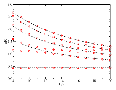
Figure 15: Spectrum of the theory for different values of the volume for the following simulation parameters, describing an inelastic scattering: $\nu=1.05$, $\lambda=0.85$, $am_{\pi,0}=0.17$. The horizontal blue dotted line shows the elastic threshold.

For Lüscher’s method the results are nonsensical, as would be expected since the method can only be demonstrated in the elastic region due to the restricitions of the Bethe-Salpeter Kernel and more fundamentally the fact that the formula is first derived in quantum mechanics.

Figure 16 shows an example of applying the method beyond the inelastic threshold for $\nu=1.0$ and $\lambda=1.4$. It can be seen that the profile does not fit what would expected of the scattering phase shift and in fact the second point after the threshold, being above $\pi/2$, could even break unitarity.

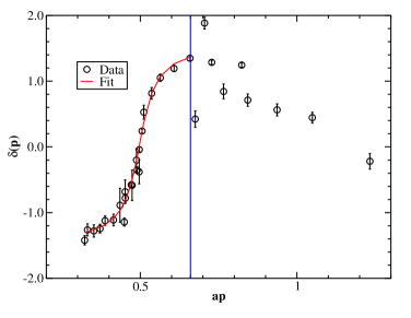
Figure 16: Inelastic data with Lüscher’s formula. For the case of $\nu=1.0$, $\lambda=1.4$, $am_{\pi,0}=0.36$. (Onset of inelastic region marked).

Fortunately for these values of $\nu$ and $\lambda$ the resonance is not above the treshold. For $\nu=1.05$, $\lambda=0.85$, where the resonance is above threshold, the problems mentioned above make the results uninterpretable. It is worth noting that in Figure 15 we do not have any hints of the expected $4\pi$ level; an explicit implementation of an interpolator should therefore be necessary.

In Figure 17 (Top) the probability distribution is shown considering the correct background and all levels. The distribution without the two levels, characterized by the absence of their own background, is shown in Figure 17 (Bottom). In this case a bad and unexpected result is obtained: a jump around $m\approx 1.13$ is present; this is a further proof of how laborious this method is.

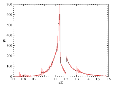
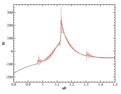
Figure 17: (Top) The probability distribution considering the correct background. (Bottom) Probability distribution $\tilde{W}$ using the correct background and excluding the two levels that are without a corresponding background. Simulation parameters: $\nu=1.05$, $\lambda=0.85$, $am_{\pi,0}=0.17$.

The background was subtracted following the same procedure as before but around $L=20a$ for the energy levels around $(1,1,1)$ a new problem arises. We have already seen that the only way to avoid a jump in the histogram $\tilde{W}$ is to make the correct correspondence at the two extremities of the volume interval ($L=8a$ and $L=20a$ in this case) between the energy levels of the interacting theory and the corresponding background. They should coincide or at least be parallel (after the lengthening of the free spectrum lines). Figure 6 (Top) demonstrates that this is exactly what happened in the previous cases; this characteristic is not present in this case. The two lines are not parallel because for $L=20a$ the effect of the interaction is too strong. Note that this problem is not related to the inelastic regime, but could be present in the previous cases as well; it is only by chance that this did not happen. The only way to avoid this new problem is to consider a different volume range. In particular we have verified that in this case a better choice is $8\leq L/a\leq 18$.

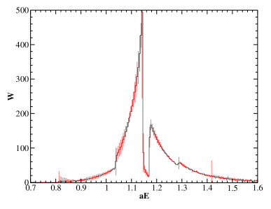
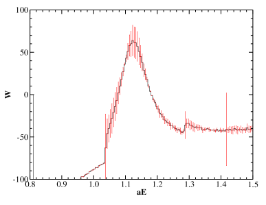
Figure 18: Like Figure 17 but considering a volume range $8\leq L/a\leq 18$ in Figure 15. Simulation parameters: $\nu=1.05$, $\lambda=0.85$, $am_{\pi,0}=0.17$.

Using this new interval we can determine the probability distribution shown in Figure 18 (Top); excluding the two levels as before we get the result of Figure 18 (Bottom). Finally, we can see a Breit-Wigner shape that we can fit as shown in Figure 19 obtaining the following parameters: $aM_{\sigma}=1.11(3)$, $a\Gamma_{\sigma}=0.11(3)$.

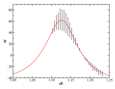
Figure 19: Data from Figure 18 (Bottom) that we fit to determine the resonance parameters with the final curve fitting. Simulation parameters: $\nu=1.05$, $\lambda=0.85$, $am_{\pi,0}=0.17$.

It is clear therefore that in the inelastic regime we can also apply exactly the same procedure as was developed for the elastic case and finally we can determine in this case the resonance parameters also. Unfortunately, in contrast with the elastic regime there is no theoretical support in this case. Therefore, even if we can determine the parameters for the Breit-Wigner shape of the probability distribution hystogram, there is no reason to link these numbers with the resonance parameters.

IV.5 Correlator method

We have also performed a preliminary investigation of a third method described in Ref Meissner et al. (2011). This method attempts to extract resonance parameters via fitting the correlator to some asymptotic form at small times. This avoids the Maiani-Testa theorem, as the theorem only restricts access to scattering information via the $n$-point functions with $n\geq 3$. Also, in using the correlator we are treating resonances on the same footing as stable states. The form of the correlator that we fit to is:

$$D(t) = \mbox{e}^{-\omega_{\sf min}t}\,\biggl{\{}c_{0}F^{(0)}(t,E_{R})+$$ (43)

$$c_{1}F^{(1)}(t,E_{R})+\sum_{k=0}^{\infty}\frac{x_{k}}{t^{l+k+3/2}}\biggr{\}}\ ,$$

$\omega_{min}$ being the value of the multiparticle threshold, which in this work is $\omega_{min}=2m_{\pi}$; $E_{R}$ is the location of the pole associated with the resonance relative to the multiparticle threshold, namely $E_{R}=\left(M_{\sigma}-\omega_{min}\right)-i\frac{\Gamma}{2}$, with $M_{\sigma}$ and $\Gamma$ the mass and width of the resonance respectively. We label the real part of $E_{R}$ as $E_{0}$ in what follows, $E_{0}=\left(M_{\sigma}-\omega_{min}\right)$.
The $F^{(i)}(t,E_{R})$ functions have the following definition:

$$F^{(0)}(t,E_{R}) = -\frac{2}{\Gamma}\,\mbox{Im}\,\chi(t,E_{R})$$

$$F^{(1)}(t,E_{R}) = \mbox{Re}\,\chi(t,E_{R})-\frac{2E_{0}}{\Gamma}\,\mbox{Im}\,\chi(t,E_{R})\ .$$ (44)

The function $\chi(t,E_{R})$ is calculated via the expression:

$$\chi(t,E_{R}) = -\pi\,\sqrt{-E_{R}}\,\mbox{e}^{-E_{R}t}+$$ (45)

$$\sqrt{\frac{\pi}{t}}\,\biggl{\{}1+\sum_{i=0}^{\infty}\,\frac{(-2E_{R}t)^{i+1}}{(2i+1)!!}\biggr{\}}\,.$$

A resonance is to be found as a pole on the second (unphysical) Riemann sheet of the Kallen-Lehmann spectral function. However since the branch cut that gives rise to this second Riemann sheet dissolves into a series of poles in finite volume, it is not obvious how the resonance can have an effect on the correlator. However if, in infinite volume, the resonance is very narrow then it is close enough to the branch cut for it to have an effect on the first (physical) Riemann sheet and so its influence will show up in the infinite volume correlator. The finite volume correlator converges to the infinite volume one rapidly at large volumes and so the influence of the resonance shows up in the finite volume correlators we observe on the lattice. We should then be able to apply Eq. 43 at large volumes. In Eq. 43 the $x_{k}$ represent the non-resonant scattering, which in our model we expect to be small. We chose the value $k=2$, as smaller values were found to give poor results. We then fitted the sigma correlator for the $L=19$ lattice for the $\nu=1.0$, $\lambda=1.4$, $am_{\pi}=0.36$ parameters and obtained the following results (the fit is shown in Fig. 20):

$$aM_{\sigma} = 1.32(5)\ ,$$

$$a\Gamma_{\sigma} = 0.107(7)\ ,$$

$$c_{0} = -0.00122(4)\ ,$$

$$c_{1} = 0.00023(8)\ ,$$

$$x_{0} = 0.078(1)\ ,$$

$$x_{1} = 0.158(5)\ .$$

The fit, which was done in the window $t\in[1,8]$, has a chi-squared per degree of freedom of $\chi^{2}/\nu=0.8362$. The resonance width $\Gamma$ appeared to quite sensitive to the fit window if values of $t$ greater than $10$ were taken. However this is possibly not a surprising result as the form for the correlator Eq. 43 is derived for small times.
It should be noted that this method obtained these results via a fit to the correlator in a single, large volume. Of course the method also introduces new fitting parameters, $c_{0},c_{1},x_{0}$ and $x_{1}$, which make the fit less discriminating. The method also appears to be restricted to narrow resonances, attempts to apply the method to the broader resonance data of this work were not succesful.
The results are however consistent with the two preceeding methods. Only a preliminary investigation of this method was made, in particular a more precise estimate of the errors via the Bayesian analysis suggested in Ref Meissner et al. (2011) might improve the situation.

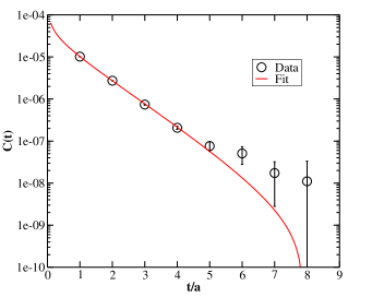
Figure 20: Fit to sigma correlator; parameters: $\nu=1.0$, $\lambda=1.4$, $am_{\pi}=0.36$.

V Conclusions and outlook

The investigation of the two methods studied in this work has elucidated their relative strengths and weaknesses when they are applied to data from a Monte Carlo study, which have finite statistical precision. Lüscher’s method requires an estimation on the functional form of the scattering phase shift, in our case we used the ansatz of the Breit-Wigner form associated to an isolated resonance. Once these two requirements are met the method is relatively straight forward to apply. The main disadvantage is the increasing errors as the resonance becomes broader and the clear restriction to studying elastic scattering.

The histogram method, since it has the form of a Breit-Wigner peak, provides a distinctive visual check of the presence of resonances. However the method of constructing a histogram from Monte Carlo data with a limited range of volumes is not as straightforward as applying Lüscher’s technique and one also finds increasing errors for broader resonances. For very broad resonances, the method misses the state entirely.

Lüscher’s method is then the stronger of the two based on our experience here due to its ease of application. For narrow resonances however, results from both techniques appear to be complimentary and have similar statistical precision. We briefly investigated a third method which makes more direct use of the time-dependence of correlator data and would treat resonances similarly to stable states, but much remains to be done to show it is useful for the analysis of Monte Carlo data.

The major drawback for all methods is that they are restricted to the elastic region. Studing the inelastic region is of crucial importance to learning more detail about the resonances that emerge from QCD. What is clear is that any more advanced method that has potential in that region will need to be able to deal with statistical uncertainty in a robust way without the need for delicate fine-tuning.

References

- Maiani and Testa (1990) L. Maiani and M. Testa, Phys.Lett. B245, 585 (1990).
- Bernard et al. (2008) V. Bernard, M. Lage, U.-G. Meissner, and A. Rusetsky, JHEP 08, 024 (2008), eprint 0806.4495.
- Meissner et al. (2011) U.-G. Meissner, K. Polejaeva, and A. Rusetsky, Nucl. Phys. B846, 1 (2011), eprint 1007.0860.
- McNeile and Michael (2003) C. McNeile and C. Michael (UKQCD), Phys. Lett. B556, 177 (2003), eprint hep-lat/0212020.
- Feng et al. (2011) X. Feng, K. Jansen, and D. B. Renner, Phys. Rev. D83, 094505 (2011), eprint 1011.5288.
- Aoki et al. (2011) S. Aoki et al. (CS), Phys. Rev. D84, 094505 (2011), eprint 1106.5365.
- Lang et al. (2011) C. B. Lang, D. Mohler, S. Prelovsek, and M. Vidmar, Phys. Rev. D84, 054503 (2011), eprint 1105.5636.
- Peardon et al. (2009) M. Peardon et al. (Hadron Spectrum), Phys. Rev. D80, 054506 (2009), eprint 0905.2160.
- Morningstar et al. (2011) C. Morningstar et al., Phys. Rev. D83, 114505 (2011), eprint 1104.3870.
- Bulava (2011) J. Bulava (2011), eprint 1112.0212.
- Hansen and Sharpe (2012) M. T. Hansen and S. R. Sharpe (2012), eprint 1204.0826.
- Briceno and Davoudi (2012) R. A. Briceno and Z. Davoudi (2012), eprint 1204.1110.
- Giudice and Peardon (2010) P. Giudice and M. J. Peardon, AIP Conf.Proc. 1257, 784 (2010), eprint 1010.1390.
- Giudice et al. (2010) P. Giudice, D. McManus, and M. Peardon, PoS LATTICE2010, 105 (2010), eprint 1009.6192.
- Lüscher (1986) M. Lüscher, Commun. Math. Phys. 105, 153 (1986).
- Lüscher (1991a) M. Lüscher, Nucl. Phys. B364, 237 (1991a).
- Morningstar (2008) C. Morningstar, PoS LATTICE2008, 009 (2008), eprint 0810.4448.
- Gockeler et al. (1994) M. Gockeler, H. A. Kastrup, J. Westphalen, and F. Zimmermann, Nucl. Phys. B425, 413 (1994), eprint hep-lat/9402011.
- DeGrand and Detar (2006) T. DeGrand and C. E. Detar, Lattice methods for quantum chromodynamics (World Scientific, 2006).
- Michael (1985) C. Michael, Nucl.Phys. B259, 58 (1985).
- Lüscher and Wolff (1990) M. Lüscher and U. Wolff, Nucl. Phys. B339, 222 (1990).
- Lüscher (1991b) M. Lüscher, Nucl. Phys. B354, 531 (1991b).