Optimal execution and price manipulations in time-varying limit order books

Abstract: This paper focuses on an extension of the Limit Order Book (LOB) model with general shape introduced by Alfonsi, Fruth and Schied [2]. Here, the additional feature allows a time-varying LOB depth. We solve the optimal execution problem in this framework for both discrete and continuous time strategies. This gives in particular sufficient conditions to exclude Price Manipulations in the sense of Huberman and Stanzl [12] or Transaction-Triggered Price Manipulations (see Alfonsi, Schied and Slynko [4]). These conditions give interesting qualitative insights on how market makers may create or not price manipulations.

Key words: Market impact model, optimal order execution, limit order book, market makers, price manipulation, transaction-triggered price manipulation.

AMS Class 2010: 91G99, 91B24, 91B26, 49K99

Acknowledgements: This work has benefited from the support of the Eurostars E!5144-TFM project and of the “Chaire Risques Financiers” of Fondation du Risque. José Infante Acevedo is grateful to AXA Resarch Fund for his doctoral fellowship.

Introduction

It is a rather standard assumption in finance to consider an infinite liquidity. By infinite liquidity, we mean here that the asset price is given by a a single value, and that one can buy or sell any quantity at this price without changing the asset price. This assumption is in particular made in the Black and Scholes model [7], and is often made as far as derivative pricing is concerned. When considering portfolio over a large time horizon, this approximation is relevant since one may split orders in small ones along the time and reduces one’s own impact on the price. At most, the lack of liquidity can be seen as an additional transaction cost. This issue has been broadly investigated in the literature, see Cetin, Jarrow and Protter [8] and references within.

If we consider instead brokers that have to trade huge volumes over a short time period (some hours or some days), we can no longer neglect the price impact of trading strategies. We have to focus on the market microstructure and model how prices are modified when buy and sell orders are executed. Generally speaking, the quotation of an asset is made through a Limit Order Book (LOB) that lists all the waiting buy and sell orders on this asset. The order prices have to be a multiple of the tick size, and orders at the same price are arranged in a First-In-First-Out stack. The bid (resp. ask) price is the price of the highest waiting buy (resp. lowest selling buy) order. Then, it is possible to buy or sell the asset in two different ways: one can either put a limit order and wait that this order matches another one or put a market order that consumes the cheapest limit orders in the book. In the first way, the transaction cost is known but the execution time is uncertain. In the second way, the execution is immediate (provided that the book contains enough orders). The price per share instead depends on the order size. For a buy (resp. sell) order, the first share will be traded at the ask (resp. bid) price while the last one will be traded some ticks upper (resp. lower) in order to fill the order size. The ask (resp. bid) price is then modified accordingly.

The typical issue on a short time scale is the optimal execution problem: on given a time horizon, how to buy or sell optimally a given amount of assets? As pointed in Gatheral [10] and Alfonsi, Schied and Slynko [4], this problem is closely related to the market viability and to the existence of price manipulations. Modelling the full LOB dynamics is not a trivial issue, especially if one wants to keep tractability to solve then the optimal execution problem. Instead, simpler models called market impact models have been proposed. These models only describe the dynamics of one asset price and model how the asset price is modified by a trading strategy. Thus, Bertsimas and Lo [6], Almgren and Chriss [5], Obizhaeva and Wang [13] have proposed different models where the price impact is proportional to the trading size, in which they solve the optimal execution problem. However, some empirical evidence on the markets show that the price impact of a trade is not proportional to its size, but is rather proportional to a power of its size (see for example Potters and Bouchaud [14], and references within). With this motivation in mind, Gatheral [10] has suggested a nonlinear price impact model. In the same direction, Alfonsi, Fruth and Schied [2] have derived a price impact model from a simple LOB modelling. Basically, the LOB is modelled by a shape function that describes the density of limit orders at a given price. This model has then been studied further by Alfonsi and Schied [3] and Predoiu, Shaikhet and Shreve [15].

The present paper extends this model by letting the LOB shape function vary along the time. Beyond solving the optimal execution problem in a more general context, our goal is to understand how the dynamics of the LOB may create or not price manipulations. Indeed, a striking result in [2, 3] is that the optimal execution strategy is made with trades of same sign, which excludes any price manipulation. This result holds under rather general assumptions on the LOB shape function, when the LOB shape does not change along the time. Instead, we will see in this paper that a time-varying LOB may induce price manipulations and we will derive sufficient conditions to exclude them. These conditions are not only interesting from a theoretical point of view. They give a qualitative understanding on how price manipulations may occur when posting or cancelling limit orders. While preparing this work, Fruth, Schöneborn and Urusov [9] have presented a paper where this issue is addressed for a block-shaped LOB, which amounts to a proportional price impact. Here, we get back their result and extend them to general LOB shapes and thus nonlinear price impact. The other contribution of this paper is that we solve the optimal execution in a continuous time setting while [2, 3] mainly focus on discrete time strategies. This is in particular much more suitable to state the conditions that exclude price manipulations.

1 Market model and the optimal execution problem

1.1 The model description

The problem that we study in this paper is the classical optimal execution problem. To deal with this problem, we consider in this paper a framework which is a natural extension of the model proposed in Alfonsi, Fruth and Schied [2] and developed by Alfonsi and Schied [3] and Predoiu, Shaikhet and Shreve [15]. The additional feature that we introduce here is to allow a time varying depth of the order book. We consider a large trader who wants to liquidate a portfolio of $\mathbbm{x}$ shares in a time period of $[0,T]$. In order liquidate these $\mathbbm{x}$ shares, the large trader uses only market orders, that is buy or sell orders that are immediately executed at the best available current price. Thus, our large trader cannot put limit orders. A long position $\mathbbm{x}>0$ will correspond to a sell program while a short position $\mathbbm{x}<0$ will stand for a a buy strategy. The optimal execution problem consists in finding the optimal trading strategy that minimizes the expected cost of the large trader.

We assume that the price process without the large trader would be given by a rightcontinuous martingale $(S^{0}_{t},t\geq 0)$ on a given filtered probability space $\left(\Omega,(\mathcal{F}_{t}),\mathcal{F},\mathbb{P}\right)$. The actual price process $(S_{t},t\geq 0)$ that takes into account the trades of the large trader is defined by:

$$S_{t}=S^{0}_{t}+D_{t},\ t\geq 0.$$ (1)

Thus, the process $(D_{t},t\geq 0)$ describes the price impact of the large trader. We also introduce the process $(E_{t},t\geq 0)$ that describes the volume impact of the large trader. If the large trader puts a market order of size $\xi_{t}$ ($\xi_{t}>0$ is a buy order and $\xi_{t}<0$ a sell order), the volume impact process changes from $E_{t}$ to:

$$E_{t+}:=E_{t}+\xi_{t}.$$ (2)

When the large trader is not active, its volume impact $E_{t}$ goes back to $0$. We assume that it decays exponentially with a deterministic time-dependent rate $\rho_{t}>0$ called resilience, so that we have:

$$dE_{t}=-\rho_{t}E_{t}dt.$$ (3)

We now have to specify how the processes $D$ and $E$ are related. To do so, we suppose a continuous distribution buy and sell limit orders around the unaffected price $S^{0}_{t}$: for $x\in\mathbb{R}$, we assume that the number of limit orders available between prices $S^{0}_{t}+x$ and $S^{0}_{t}+x+dx$ is given by $\lambda(t)f(x)dx$. These orders are sell orders if $x\geq D_{t}$ and buy orders otherwise. The functions $f:\mathbb{R}\mapsto(0,\infty)$ and $\lambda:[0,T]\mapsto(0,\infty)$ are assumed to be continuous, and represent respectively the LOB shape and the depth of the order book. We define the antiderivative of the function $f$, $F(y):=\int^{y}_{0}f(x)dx,\;\;y\in\mathbb{R},$ and assume that

$$\underset{x\rightarrow-\infty}{\lim}F(x)=-\infty\text{ and }\underset{x\rightarrow\infty}{\lim}F(x)=\infty,$$ (4)

which means that the book contains an infinite number of limit buy and sell orders. Thus, we set the following relationship between the volume impact $E_{t}$ and the price impact $D_{t}$:

$$\int^{D_{t}}_{0}\lambda(t)f(x)dx=E_{t},$$

or equivalently,

$$E_{t}=\lambda(t)F(D_{t})\text{ and }D_{t}=F^{-1}\left(\frac{E_{t}}{\lambda(t)}\right).$$ (5)

Within this framework, a large trade $\xi_{t}$ changes $D_{t}$ to $D_{t+}=F^{-1}\left(\frac{E_{t}+\xi_{t}}{\lambda(t)}\right)$ and has the cost

$$\int_{D_{t}}^{D_{t+}}(S^{0}_{t}+x)\lambda(t)f(x)dx=\xi_{t}S^{0}_{t}+\int_{D_{t}}^{D_{t+}}\lambda(t)xf(x)dx:=\pi_{t}(\xi_{t}).$$ (6)

Throughout the paper, we assume that $\lambda$ is $\mathcal{C}^{2}$ and set $\eta_{t}=\frac{\lambda^{\prime}(t)}{\lambda(t)}$. Thus, we have

$$\lambda(t)=\lambda(0)\exp\left(\int_{0}^{t}\eta_{u}du\right),$$

and $t\mapsto\eta_{t}$ is $\mathcal{C}^{1}$. Similarly, we assume that $t\mapsto\rho_{t}$ is $\mathcal{C}^{1}$.

Now, let us observe that we have assumed that the volume impact decays exponentially when the large trader is inactive. Other choices are of course possible, and a natural one would be to assume that the price impact decays exponentially

$$dD_{t}=-\rho_{t}D_{t}dt,$$ (7)

which amounts to assume that $dE_{t}=\eta_{t}E_{t}dt-\rho_{t}\lambda(t)f(F^{-1}(E_{t}/\lambda(t)))F^{-1}(E_{t}/\lambda(t))dt$ by (5).

Definition 1.1.

The dynamics of “model $V$” with volume impact reversion is the one given by (1), (2), (3) and (5). The dynamics of “model $P$” with price impact reversion is the one given by (1), (2), (7) and (5). In both models, we assume that the market is at equilibrium at time $0$, i.e. $E_{0}=D_{0}=0$.

Remark 1.1.

Though being simplistic, this model describes through $\rho_{t}$ and $\lambda(t)$ the two different ways that market makers have to put (or cancel) limit orders: it is either possible to pile orders at an existing price or to put orders at a better price than the existing ones. Thus, $\lambda(t)$ describes how market makers pile orders while $\rho_{t}$ describes the rate at which new orders appear at a better price. Basically, one may think these functions one-day periodic, with relative high values at the opening and the closing of the market and low values around noon. The particular case $\lambda\equiv 1$ corresponds to the model introduced by Alfonsi, Fruth and Schied [2] for which new orders can only appear at a better price.

1.2 The optimal execution problem, and price manipulation strategies

We focus on the optimal liquidation of a portfolio with $\mathbbm{x}$ shares by a large trader who can place market orders over a period of time $[0,T]$. Thus, $\mathbbm{x}>0$ (resp. $\mathbbm{x}<0$) corresponds to a selling (resp. buying) strategy.

We first consider discrete strategies and assume that at most $N+1$ trades can occur. An admissible strategy will be then described by an increasing sequence $\tau_{0}=0\leq\dots\leq\tau_{N}=T$ of stopping times and random variables $\xi_{0},\dots,\xi_{N}$ ($\xi_{i}$ stands for the trading size at time $\tau_{i}$) such that

• $\mathbbm{x}+\sum_{i=0}^{N}\xi_{i}=0$, i.e. the trader liquidates indeed $\mathbbm{x}$ shares,

• $\xi_{i}$ is $\mathcal{F}_{\tau_{i}}$-measurable,

• $\exists M\in\mathbb{R},\forall 0\leq i\leq N,\xi_{i}\geq M$, a.s.

The expected cost of an admissible strategy $({\bm{\xi}},\mathcal{T})$ with ${\bm{\xi}}=(\xi_{0},\dots,\xi_{N})$ and $\mathcal{T}=(\tau_{0},\dots,\tau_{N})$ is given by

$$\mathcal{C}({\bm{\xi}},\mathcal{T})=\mathbb{E}\left[\sum_{i=0}^{N}\pi_{\tau_{i}}(\xi_{i})\right],$$ (8)

where $\pi_{\tau_{i}}(\xi_{i})$ stands for the cost of the $i$-th trade, and is defined by (6) in models $V$ or $P$. The goal of the large trader is then to minimize this expected cost among the admissible strategies.

We also consider continuous time trading strategy and make the same assumptions as Gatheral et al. [11]. An admissible strategy $(X_{t})_{t\geq 0}$ is a stochastic process such that

• $X_{0}=\mathbbm{x}$ and $X_{T+}=0$,

• $X$ is $(\mathcal{F}_{t})$-adapted and leftcontinuous,

• the function $t\in[0,T+]\mapsto X_{t}$ has finite and a.s. bounded total variation.

The process $X_{t}$ describes the number of shares that remains to liquidate at time $t$. Thus, the discrete time strategy above corresponds to $X_{t}=\mathbbm{x}+\sum_{i=0}^{N}\xi_{i}\mathbf{1}_{\tau_{i}<t}$, and the three assumptions on $({\bm{\xi}},\mathcal{T})$ precisely give the ones on $X$. Let us observe that processes $E$ and $D$ are also leftcontinuous since we have in model $V$ (resp. model $P$):

$$dE_{t}=dX_{t}-\rho_{t}E_{t}dt,\ (\text{resp.}\ dE_{t}=dX_{t}+\eta_{t}E_{t}dt-\rho_{t}\lambda(t)f(F^{-1}(E_{t}/\lambda(t)))F^{-1}(E_{t}/\lambda(t))dt).$$ (9)

We want now to write the cost associated to the strategy $X$. To do so, we introduce the following notations

$$x\in\mathbb{R},\tilde{F}(x)=\int^{x}_{0}yf(y)dy,\ G(x)=\tilde{F}\left(F^{-1}(x)\right),$$ (10)

so that $\pi_{t}(dX_{t})=S^{0}_{t}dX_{t}+\lambda(t)[G\left(\frac{E_{t}+dX_{t}}{\lambda(t)}\right)-G\left(\frac{E_{t}}{\lambda(t)}\right)]$. Since $G^{\prime}=F^{-1}$, the cost of an admissible strategy is given by:

$$\mathcal{C}(X)=\mathbb{E}\left[\int_{0}^{T}\left[S^{0}_{t}+F^{-1}\left(\frac{E_{t}}{\lambda(t)}\right)\right]dX_{t}+\sum_{t\leq T}\lambda(t)\left[G\left(\frac{E_{t}+\Delta X_{t}}{\lambda(t)}\right)-G\left(\frac{E_{t}}{\lambda(t)}\right)-F^{-1}\left(\frac{E_{t}}{\lambda(t)}\right)\Delta X_{t}\right]\right],$$ (11)

which coincides with (8) for discrete strategies. Here, $\Delta X_{t}=X_{t+}-X_{t}$ denotes the jump of $X$ at time $t$ (jumps are countable), and $dX_{t}$ stands for the signed measure on $[0,T]$ associated to $(X_{t},0\leq t\leq T+)$ (a jump $\Delta X_{T}$ induces a Dirac mass in $T$). If we introduce the continuous part of $X$, $X^{c}_{t}:=X_{t}-\sum_{0\leq s<t}\Delta X_{s}$, we can rewrite the cost as follows:

$$\mathcal{C}(X)=\mathbb{E}\left[\int_{0}^{T}\left[S^{0}_{t}+F^{-1}\left(\frac{E_{t}}{\lambda(t)}\right)\right]dX^{c}_{t}+\sum_{t\leq T}S^{0}_{t}\Delta X_{t}+\lambda(t)\left[G\left(\frac{E_{t}+\Delta X_{t}}{\lambda(t)}\right)-G\left(\frac{E_{t}}{\lambda(t)}\right)\right]\right].$$ (12)

The optimal execution problem is in fact closely related to questions around market viability and arbitrage. We recall the definition of price manipulation strategies introduced by Huberman and Stanzl [12].

Definition 1.2.

A round trip is an admissible strategy $X$ for $\mathbbm{x}=0$. A Price Manipulation Strategy (PMS) in the sense of Huberman and Stanzl is a round trip whose expected cost is negative, i.e. $\mathcal{C}(X)<0$.

Heuristically, if a PMS exists, it could be repeated indefinitely and would lead to a classical arbitrage (i.e. an almost sure profit) by a law of large numbers. However, it has been pointed in Alfonsi et al. [4] the absence of PMS does not ensure the market stability. In fact, in some PMS free models, the optimal strategy to sell $\mathbbm{x}$ shares consists in buying and selling successively a much higher amount of shares. To correct this, they introduce the following definition.

Definition 1.3.

A model admits transaction-triggered price manipulations (TTPM) if the expected cost of a sell (buy) program can be decreased by intermediate buy (sell) trades, i.e.

$$\exists X\text{ admissible},\ \mathcal{C}(X)<\inf\left\{\mathcal{C}(\tilde{X}),\tilde{X}\text{ is admissible and nonincreasing or nondecreasing}\right\}.$$

It is rather natural choice to exclude TTPM: in presence of TTPM a large trader would increase the traded volume to minimize its cost, which produce noise and may yield to instability. Besides, the absence of TTPM implies the absence of PMS. The optimal strategy for buying $\varepsilon>0$ shares is made only with intermediate buy trades and has thus a positive cost. Thus, by some cost continuity that usually holds (this is the case for models $V$ and $P$), any round trip has a nonnegative cost.

Remark 1.2.

It is possible to define a two-sided limit order book model like in Alfonsi, Fruth and Schied [2] or Alfonsi and Schied ([3], Section 2.6). In such a model, bid and ask prices evolve as follows. A buy (resp. sell) order of the large trader shifts the ask (resp. bid) price and leaves the bid (resp. ask) price unchanged. When the large trader is idle, the shifts on the ask and bid prices goes back exponentially to zero, like in models $V$ or $P$. As in [2, 3], the two-sided model coincides with the model presented here when the large trader puts only buy orders or only sell orders. In particular, the optimal strategies are the same in both models in absence of TTPM.

2 Main results

The first focus of this paper is to extend the results obtained in Alfonsi et al. [2, 3] and obtain the optimal execution strategies for LOB with a time varying depth $\lambda$. Doing so, our goal is also to better understand how this time varying depth may create manipulation strategies. In fact, it was shown in [2] and [3] for $\lambda\equiv 1$ that under some general assumptions on the shape function $f$, there is an optimal liquidation strategy which is made only with sell (resp. buy) orders when $\mathbbm{x}>0$ (resp. $\mathbbm{x}<0$). Thus, there is no PMS nor TTPM when the LOB shape is constant. This is a striking result, and one may wonder how this is modified by changing slightly the assumptions. In Alfonsi, Schied and Slynko [4] is studied the case of a block-shaped LOB, where the resilience is not exponential so that the market has some memory of the past trades. Conditions on the market resilience are given to exclude PMS and TTPM. Analogously, we want to obtain here conditions on $\lambda$ and $\rho$ that rules out such strategies. This is not only interesting from a theoretical point of view. This will give also some noticeable qualitative insights for market makers. In fact, for a market maker who places and cancels significant limit orders, these conditions will indicate if he may or not create manipulation strategies.

Before showing the results, it is worth to make further derivations on the expected cost. Let us start with discrete strategies. By using the martingale property on $S^{0}$ and the assumptions on ${\bm{\xi}}$ made in Section 1.2, we can show easily like in [3] that

$$\mathcal{C}({\bm{\xi}},\mathcal{T})=-S^{0}_{0}\mathbbm{x}+\mathbb{E}\left[\sum_{i=0}^{N}\int_{D_{\tau_{i}}}^{D_{\tau_{i}+}}\lambda(\tau_{i})xf(x)dx\right].$$

Then, it is easy to check that $\sum_{i=0}^{N}\int_{D_{\tau_{i}}}^{D_{\tau_{i}+}}\lambda(\tau_{i})xf(x)dx$ is a deterministic function of $({\bm{\xi}},\mathcal{T})$ in both volume impact reversion and price impact reversion models. We respectively denote by $C^{V}({\bm{\xi}},\mathcal{T})$ and $C^{P}({\bm{\xi}},\mathcal{T})$ this function and get:

$$\mathcal{C}({\bm{\xi}},\mathcal{T})=-S^{0}_{0}\mathbbm{x}+\mathbb{E}\left[C^{M}({\bm{\xi}},\mathcal{T})\right],$$ (13)

where $M\in\{V,P\}$ indicates the model chosen. Thus, if the function $({\bm{x}},{\bm{t}})\mapsto C^{M}({\bm{x}},{\bm{t}})$ has a unique minimizer on $\{({\bm{x}},{\bm{t}})\in\mathbb{R}^{N}\times\mathbb{R}^{N+1},\sum_{i=1}^{N}x_{i}=-\mathbbm{x},0=t_{0}\leq\dots\leq t_{N}=T\}$, the optimal strategy is deterministic and given by this minimizer. When $\lambda$ is constant, it is shown in [3] that under some assumptions on $f$ depending on the model chosen, the optimal time grid ${\bm{t}}^{\star}$ is homogeneous with respect to $\rho$, i.e. $\int_{t_{i}^{\star}}^{t_{i+1}^{\star}}\rho_{s}ds=\frac{1}{N}\int_{0}^{T}\rho_{s}ds$. Instead, there is no such a simple characterization for general $\lambda$, even in the block-shaped case. Thus, we will focus on optimizing the trading strategy ${\bm{\xi}}$ on a fixed time grid ${\bm{t}}$:

$${\bm{t}}=(t_{0},\dots,t_{N}),\text{ such that $0=t_{0}<\dots<t_{N}=T$}.$$ (14)

Last, we introduce the following notations that will be used throughout the paper:

$$a_{i}=e^{-\int^{t_{i}}_{t_{i-1}}\rho_{u}du},\ \tilde{a}_{i}=\frac{a_{i}\lambda(t_{i-1})}{\lambda(t_{i})}=e^{-\int^{t_{i}}_{t_{i-1}}(\rho_{u}+\eta_{u})du},\ \hat{a}_{i}=a_{i}\frac{\lambda(t_{i})}{\lambda(t_{i-1})}=e^{-\int^{t_{i}}_{t_{i-1}}(\rho_{u}-\eta_{u})du},\ \ \ 1\leq i\leq N.$$ (15)

Similarly in the continuous case, we get by using the martingale assumption (see Lemma 2.3 in Gatheral, Schied and Slynko [11]) that $\mathbb{E}[\int_{0}^{T}S^{0}_{t}dX_{t}]=-\mathbbm{x}S^{0}_{0}$. From (11) and (12), we get $\mathcal{C}(X)=-\mathbbm{x}S^{0}_{0}+\mathbb{E}[C^{M}(X)]$, where

$$C^{M}(X)=\int_{0}^{T}F^{-1}\left(\frac{E_{t}}{\lambda(t)}\right)dX^{c}_{t}+\sum_{t\leq T}\lambda(t)\left[G\left(\frac{E_{t}+\Delta X_{t}}{\lambda(t)}\right)-G\left(\frac{E_{t}}{\lambda(t)}\right)\right].$$

Once again, $C^{M}$ is a deterministic function of the strategy $X$ in both models $M\in\{V,P\}$, and it is sufficient to focus on its minimization.

2.1 The block-shaped LOB case ($f\equiv 1$)

In this section, we consider a shape function of the limit order book that has the form $\lambda(t)$. This time-dependent framework generalizes the block-shaped limit order book case studied by Obizhaeva and Wang [13] that consists in considering a uniform distribution of shares with respect to the price. We will get an explicit solution for the optimal execution problem, which extends the results given by Alfonsi, Fruth and Schied [1].

2.1.1 Volume impact reversion model

When $f\equiv 1$, the deterministic cost function is simply given by

$$C^{V}({\bm{\xi}},{\bm{t}})=\sum^{N}_{n=0}\lambda(t_{n})\int^{D_{t_{n}+}}_{D_{t_{n}}}xf(x)dx=\sum^{N}_{i=0}\frac{\xi_{i}}{2}\left(\frac{\xi_{i}}{\lambda\left(t_{i}\right)}+2\frac{\sum_{j<i}e^{-\int^{t_{i}}_{t_{j}}\rho_{s}ds}\xi_{j}}{\lambda(t_{i})}\right),$$ (16)

which is a quadratic form: $C^{V}({\bm{\xi}},{\bm{t}})=\frac{1}{2}{\bm{\xi}}^{T}M^{V}{\bm{\xi}}$, with $M^{V}_{i,j}=\frac{\exp\left(-\left|\int_{t_{i}}^{t_{j}}\rho_{s}ds\right|\right)}{\lambda(t_{i}\vee t_{j})}$, $0\leq i,j\leq N$.

Theorem 2.1.

The quadratic form (16) is positive definite if and only if

$$a_{i}\tilde{a}_{i}<1,\forall i\in\left\{1,\ldots,N\right\}.$$ (17)

In this case, the optimal execution problem to liquidate $\mathbbm{x}$ shares on the time-grid (14) admits a unique optimal strategy ${\bm{\xi}}^{\star}$ which is deterministic and explicitly given by:

$$\begin{cases}\xi^{\star}_{0}&=-\frac{\mathbbm{x}}{K_{V}}\lambda(t_{0})\frac{1-a_{1}}{1-a_{1}\tilde{a}_{1}}\\ \xi^{\star}_{i}&=-\frac{\mathbbm{x}}{K_{V}}\lambda(t_{i})\left[\frac{a_{i+1}}{1-a_{i+1}\tilde{a}_{i+1}}(\tilde{a}_{i+1}-1)+\frac{1-\tilde{a}_{i}}{1-a_{i}\tilde{a}_{i}}\right],\ 1\leq i\leq N-1\\ \xi^{\star}_{N}&=-\frac{\mathbbm{x}}{K_{V}}\lambda(t_{N})\frac{1-\tilde{a}_{N}}{1-a_{N}\tilde{a}_{N}},\end{cases}$$ (18)

where

$$K_{V}=\frac{\lambda\left(t_{0}\right)\left(1-2a_{1}\right)+\lambda\left(t_{1}\right)}{1-a_{1}\tilde{a}_{1}}+\sum^{N}_{i=2}\lambda(t_{i})\frac{(1-\tilde{a}_{i})^{2}}{1-a_{i}\tilde{a}_{i}}.$$

Its cost is given by $C^{V}({\bm{\xi}}^{\star},{\bm{t}})=\mathbbm{x}^{2}/(2K_{V})$.

This theorem provides an explicit optimal strategy for the large trader. It also gives explicit conditions that exclude or create PMS. First, let us assume that

$$\forall t\geq 0,\ 2\rho_{t}+\eta_{t}\geq 0.$$ (19)

Then, for any time grid (14), $a_{i}\tilde{a}_{i}\leq 1$ and the quadratic form (16) is positive semidefinite since it is a limit of positive definite quadratic forms. Thus, the model is PMS free. Conversely let us assume that $2\rho_{t_{1}}+\eta_{t_{1}}<0$ for some $t_{1}\geq 0$. Let us consider the following round trip on the time grid ${\bf t}=(0,t_{1},t_{2})$ with $t_{2}>t_{1}$, where the large trader buys $x>0$ at time $t_{1}$ and sells $x$ at time $t_{2}$. The cost of such a strategy is given by

$$C^{V}((0,x,-x),{\bm{t}})=\frac{x^{2}}{2\lambda(t_{2})}\left(e^{\int^{t_{2}}_{t_{1}}\eta_{u}du}+1-2e^{-\int^{t_{2}}_{t_{1}}\rho_{u}du}\right)\underset{t_{2}\rightarrow t_{1}}{=}\frac{x^{2}}{2\lambda(t_{1})}\left((2\rho_{t_{1}}+\eta_{t_{1}})(t_{2}-t_{1})+o(t_{2}-t_{1})\right)$$ (20)

and is negative when $t_{2}$ is close enough to $t_{1}$.

Corollary 2.1.

In a block-shaped LOB, model $V$ does not admit price manipulation in the sense of Huberman and Stanzl if and only if (19) holds.

Let us now discuss this result from the point of view of market makers. A market maker that puts a significant orders may have an influence on $\rho_{t}$ and $\eta_{t}$ and can increase (resp. decrease) them by respectively adding (resp. canceling) an order at a better price or at an existing limit order price. What comes out from (19) is that no PMS may arise if one adds limit orders, whatever the way of adding new orders. Instead, PMS can occurs when canceling orders. A different conclusion will hold in the price reversion model.

An analogous result to Corollary 2.1 is stated in a recent paper by Fruth, Schöneborn and Urusov [9] that has been published while we were preparing this work. To be precise, results in [9] are given for model $P$ with a block-shaped LOB, and the optimal execution strategy is obtained in a continuous time setting. As we will see in the next paragraph, models $V$ and $P$ are mathematically equivalent when the LOB shape is constant, even though they are different from a financial point of view. By taking a regular time-grid $t_{i}=\frac{iT}{N},i=0\ldots,N$, and letting $N\rightarrow+\infty$, we get back the optimal strategy in continuous time (that we still denote by $\xi^{\star}$, by a slight abuse of notations):

$$\begin{cases}{\mathbf{\xi}^{\star}_{0}}\underset{N\rightarrow+\infty}{\longrightarrow}\xi^{\star}_{0}:=-\frac{\mathbbm{x}}{\lambda\left(T\right)+\int^{T}_{0}\frac{\rho^{2}_{s}\lambda(s)}{\eta_{s}+2\rho_{s}}ds}\frac{\lambda(0)\rho_{0}}{2\rho_{0}+\eta_{0}}\\ \frac{\mathbf{\xi}^{\star}_{i_{N}}}{T/N}\underset{N\rightarrow+\infty}{\longrightarrow}\xi^{\star}_{t}:=-\frac{\mathbbm{x}}{\lambda\left(T\right)+\int^{T}_{0}\frac{\rho^{2}_{s}\lambda(s)}{\eta_{s}+2\rho_{s}}ds}\lambda(t)\left[\left(\frac{\rho_{t}}{2\rho_{t}+\eta_{t}}\right)^{\prime}+\rho_{t}\left(\frac{\rho_{t}+\eta_{t}}{2\rho_{t}+\eta_{t}}\right)\right]\text{, for }i_{N}\text{ such that }\frac{t_{i_{N}}}{N}\underset{\Delta t\rightarrow 0}{\longrightarrow}t\\ \mathbf{\xi}^{\star}_{N}\underset{N\rightarrow+\infty}{\longrightarrow}\xi^{\star}_{T}:=-\frac{\mathbbm{x}}{\lambda\left(T\right)+\int^{T}_{0}\frac{\rho^{2}_{s}\lambda(s)}{\eta_{s}+2\rho_{s}}ds}\frac{\lambda(T)\left(\eta_{T}+\rho_{T}\right)}{\eta_{T}+2\rho_{T}}.\end{cases}$$ (21)

The strategy $dX^{\star}_{t}={\xi^{\star}_{0}}\delta_{0}(dt)+\xi^{\star}_{t}dt+{\xi^{\star}_{T}}\delta_{T}(dt)$ with initial trade ${\xi^{\star}_{0}}$, continuous trading ${\xi^{\star}_{t}}$ on $[t,t+dt]$ for $t\in(0,T)$ and last trade ${\xi^{\star}_{T}}$ is indeed shown to be optimal in Fruth, Schöneborn and Urusov [9] among the continuous time strategies with bounded variation. We will show here again this result for more general LOB shape. The optimal strategy has the following cost:

$$\frac{\mathbbm{x}^{2}}{2\left[\lambda\left(T\right)+\int^{T}_{0}\frac{\rho^{2}_{s}\lambda(s)}{2\rho_{s}+\eta_{s}}ds\right]}.$$

Besides, this provides a necessary and sufficient condition to exclude transaction-triggered price manipulation.

Corollary 2.2.

In a block-shaped LOB, model $V$ does not admit transaction-triggered price manipulation if and only if

$$\forall t\geq 0,\ \eta_{t}+\rho_{t}\geq 0,\ \text{and }\left(\frac{\rho_{t}}{2\rho_{t}+\eta_{t}}\right)^{\prime}+\rho_{t}\left(\frac{\rho_{t}+\eta_{t}}{2\rho_{t}+\eta_{t}}\right)\geq 0.$$ (22)

The first condition comes from the last trade and implies (19) since $\rho_{t}\geq 0$. It can be interpreted similarly as condition (19) from market makers’ point of view. The second condition in (22) comes from the intermediate trades and brings on the derivatives of $\rho$ and $\eta$. It is harder to get an intuitive idea of its meaning from a market maker’s point of view. Last, let us mention that we can show that the optimal strategy on the discrete time-grid (14) is made with nonnegative trades if one has (17) and

$$\frac{1-\tilde{a}_{i}}{1-a_{i}\tilde{a}_{i}}\geq a_{i+1}\frac{1-\tilde{a}_{i+1}}{1-a_{i+1}\tilde{a}_{i+1}},\;\;\forall i\in\left\{1,\ldots,N-1\right\}\text{ and }\tilde{a}_{N}\leq 1.$$ (23)

Condition (22) can be seen as the continuous time limit of condition (23).

Let us give now an illustration of the optimal strategy with a time-varying depth. We consider the case of a time-varying depth

$$\lambda(t)=\lambda_{0}+\cos(2\pi t),\text{ with }\lambda_{0}>1,$$

which corresponds to a one-day periodic function with high values at the beginning and at the end of the day. We can show that $\eta_{t}\geq-\frac{2\pi}{\sqrt{\lambda_{0}^{2}-1}}$ and with a constant resilience $\rho$, there is no PMS as soon as $2\rho-\frac{2\pi}{\sqrt{\lambda_{0}^{2}-1}}\geq 0$. Figure 1 shows the optimal execution strategy (18) with a value $\lambda_{0}$ that exclude PMS but allows TTPM. The optimal strategy to buy $50$ shares consists in buying almost $95$ shares and selling $45$ shares, which roughly treble the traded volume.

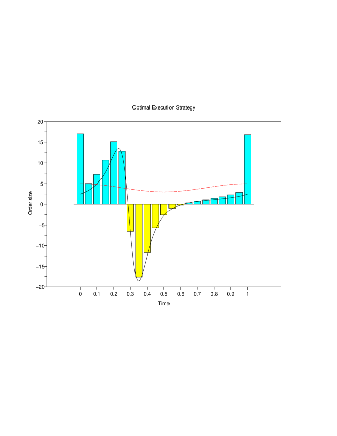
Figure 1: Optimal execution strategy to buy $50$ shares on a regular time grid, with $N=20$, $\rho=1$, $\lambda(t)=4+\cos(2\pi t)$ (plotted in dashed line). In solid line is plotted the function $t\mapsto\left(\frac{\rho_{t}}{2\rho_{t}+\eta_{t}}\right)^{\prime}+\rho_{t}\left(\frac{\rho_{t}+\eta_{t}}{2\rho_{t}+\eta_{t}}\right)$.

2.1.2 Price impact reversion model

When $f\equiv 1$, the deterministic cost function $\sum_{i=0}^{N}\int_{D_{t_{i}}}^{D_{t_{i}+}}\lambda(t_{i})xf(x)dx$ is given by

$$C^{P}({\bm{\xi}},{\bm{t}})=\sum^{N}_{n=0}\lambda(t_{n})\int^{D_{t_{n}+}}_{D_{t_{n}}}xf(x)dx=\sum^{N}_{i=0}\frac{\xi_{i}}{2}\left(\frac{\xi_{i}}{\lambda(t_{i})}+2\sum_{j<i}e^{-\int^{t_{i}}_{t_{j}}\rho_{s}ds}\frac{\xi_{j}}{\lambda(t_{j})}\right).$$ (24)

This is a quadratic form: $C^{P}({\bm{\xi}},{\bm{t}})=\frac{1}{2}{\bm{\xi}}^{T}M^{P}{\bm{\xi}}$, with $M^{P}_{i,j}=\frac{\exp\left(-\left|\int^{t_{i}}_{t_{j}}\rho_{s}ds\right|\right)}{\lambda(t_{i}\wedge t_{j})}$ for $0\leq i,j\leq N$. When $f\equiv 1$, we get from (9) that model $P$ is equivalent to model $V$ with a resilience $\tilde{\rho}_{t}=\rho_{t}-\eta_{t}$. Another way to see that both models are mathematically the same in the block-shape case is to reverse the time and consider:

$$\forall t\in[0,T],\ \hat{\rho}_{t}=\rho_{T-t},\;\hat{\lambda}(t)=\lambda(T-t)\text{ and }\hat{t}_{N-i}=T-t_{i},\text{ for }0\leq i\leq N.$$

Then, we have

$$M^{P}_{i,j}=\frac{e^{-|\int^{t_{i}}_{t_{j}}\rho_{s}ds|}}{\lambda(t_{i}\land t_{j})}=\frac{e^{-|\int^{\hat{t}_{N-j}}_{\hat{t}_{N-i}}\hat{\rho}_{s}ds|}}{\hat{\lambda}(\hat{t}_{N-i}\lor\hat{t}_{N-j})},$$ (25)

and the optimal execution problem in Model $P$ with resilience $\rho$, LOB depth $\lambda(t)$ and time-grid ${\bm{t}}$ is the same as the optimal execution problem in Model $V$ with resilience $\hat{\rho}$, LOB depth $\hat{\lambda}(t)$ and time-grid $\hat{\bm{t}}$. We immediately get the following results.

Theorem 2.2.

The quadratic form (24) is positive definite if and only if

$$a_{i}\hat{a}_{i}<1,\forall i\in\left\{1,\ldots,N\right\}$$ (26)

In this case, the optimal execution problem to liquidate $\mathbbm{x}$ shares on the time-grid (14) admits a unique optimal strategy ${\bm{\xi}}^{\star}$ which is deterministic and explicitly given by:

$$\begin{cases}\mathbf{\xi}^{\star}_{0}=-\frac{\mathbbm{x}}{K_{P}}\lambda(t_{0})\frac{1-\hat{a}_{1}}{1-a_{1}\hat{a}_{1}}.\\ \mathbf{\xi}^{\star}_{i}=-\frac{\mathbbm{x}}{K_{P}}\lambda(t_{i})\left[\frac{a_{i}}{1-a_{i}\hat{a}_{i}}(\hat{a}_{i}-1)+\frac{1-\hat{a}_{i+1}}{1-a_{i+1}\hat{a}_{i+1}}\right],\ 1\leq i\leq N-1\\ \mathbf{\xi}^{\star}_{N}=-\frac{\mathbbm{x}}{K_{P}}\lambda(t_{N})\frac{1-a_{N}}{1-a_{N}\hat{a}_{N}}\end{cases}$$ (27)

where

$$K_{P}=\frac{\lambda(t_{N})(1-2a_{N})+\lambda(t_{N-1})}{1-a_{N}\hat{a}_{N}}+\sum^{N-2}_{i=0}\lambda(t_{i})\frac{(1-\hat{a}_{i+1})^{2}}{1-a_{i+1}\hat{a}_{i+1}}.$$

Its cost is given by $C^{P}({\bm{\xi}}^{\star},{\bm{t}})=\mathbbm{x}^{2}/(2K_{P})$.

By taking a regular time-grid $t_{i}=\frac{iT}{N},i=0\ldots,N$, and letting $N\rightarrow+\infty$, we get the optimal strategy in continuous time:

$$\begin{cases}{\xi^{\star}_{0}}\underset{N\rightarrow\infty}{\longrightarrow}\xi^{\star}_{0}:=-\frac{\mathbbm{x}}{\lambda(0)+\int^{T}_{0}\frac{\rho^{2}_{s}\lambda(s)}{2\rho_{s}-\eta_{s}}ds}\lambda(0)\frac{\rho_{0}-\eta_{0}}{2\rho_{0}-\eta_{0}}\\ \frac{\xi^{\star}_{i{{}_{N}}}}{T/N}\underset{N\rightarrow\infty}{\longrightarrow}\xi^{\star}_{t}:=-\frac{\mathbbm{x}}{\lambda(0)+\int^{T}_{0}\frac{\rho^{2}_{s}\lambda(s)}{2\rho_{s}-\eta_{s}}ds}\lambda(t)\left[\left(\frac{\rho_{t}-\eta_{t}}{2\rho_{t}-\eta_{t}}\right)^{\prime}+\rho_{t}\left(\frac{\rho_{t}-\eta_{t}}{2\rho_{t}-\eta_{t}}\right)\right]\text{, for }i_{N}\text{ such that }\frac{Ti_{N}}{N}\underset{\Delta t\rightarrow 0}{\longrightarrow}t\\ \xi^{\star}_{N}\underset{N\rightarrow\infty}{\longrightarrow}\xi^{\star}_{T}:=-\frac{\mathbbm{x}}{\lambda(0)+\int^{T}_{0}\frac{\rho^{2}_{s}\lambda(s)}{2\rho_{s}-\eta_{s}}ds}\lambda(T)\frac{\rho_{T}}{2\rho_{T}-\eta_{T}}.\end{cases}$$ (28)

The strategy with initial trade ${\xi^{\star}_{0}}$, continuous trading ${\xi^{\star}_{t}}$ on $[t,t+dt]$ for $t\in(0,T)$ and last trade ${\xi^{\star}_{T}}$ is shown to be optimal in Fruth, Schöneborn and Urusov [9] among the continuous time strategies with bounded variation, and has the following cost:

$$\frac{\mathbbm{x}^{2}}{2\left[\lambda\left(0\right)+\int^{T}_{0}\frac{\rho^{2}_{s}\lambda(s)}{2\rho_{s}-\eta_{s}}ds\right]}.$$

Corollary 2.3.

In a block-shaped LOB, model $P$ does not admit price manipulation in the sense of Huberman and Stanzl if and only if

$$\forall t\geq 0,\ 2\rho_{t}-\eta_{t}\geq 0.$$ (29)

It does not admit transaction-triggered price manipulation if and only if

$$\forall t\geq 0,\ \rho_{t}-\eta_{t}\geq 0,\ \text{and }\left(\frac{\rho_{t}-\eta_{t}}{2\rho_{t}-\eta_{t}}\right)^{\prime}+\rho_{t}\left(\frac{\rho_{t}-\eta_{t}}{2\rho_{t}-\eta_{t}}\right)\geq 0.$$ (30)

The first condition in (30) comes from the initial trade while the second comes from intermediate trades. From market makers’ point of view, (29) and the first condition in (30) give different conclusions from model $V$. A significant market maker will not create manipulation strategy if he puts orders at a better price (which increases $\rho$) or cancels orders at existing prices (which decreases $\eta$). Instead, he may create manipulation strategies if he piles orders at existing prices, or if he cancels orders that are among the best offers. The second condition of (30) brings on the dynamics of $\eta$ and $\rho$ and it is more difficult to give its heuristic meaning in terms of trading. Last, let us mention that the optimal strategy in discrete time given by Theorem 2.2 is made only with trades of same sign if, and only if, one has (26) and

$$\frac{1-\hat{a}_{i+1}}{1-a_{i+1}\hat{a}_{i+1}}\geq a_{i}\frac{1-\hat{a}_{i}}{1-a_{i}\hat{a}_{i}},\;\;\forall i\in\left\{1,\ldots,N-1\right\}\text{ and }\hat{a}_{1}<1.$$ (31)

2.2 Results for general LOB shape

We extend in this section the results obtained on the optimal execution for block-shaped LOB to more general shapes. In particular, the necessary and sufficient conditions that we have obtained to exclude TTPM (namely (22) for model $V$ and (30) for model $P$) are still sufficient conditions to exclude TTPM for a wider class of shape functions. From a mathematical point of view, the approach is the same. We first characterize the optimal strategy on a discrete time grid, by using Lagrange multipliers. Then, one can guess the optimal continuous time strategy, and we prove its optimality by a verification argument.

2.2.1 Volume impact reversion model

We first introduce the following assumption that will be useful to study the optimal discrete strategy.

Assumption 2.1.

1. The shape function $f$ satisfies the following condition:

   $$f\text{ is nondecreasing on }\mathbb{R_{-}}\text{ and nonincreasing on }\mathbb{R_{+}}$$

2. $\forall t\geq 0,\rho_{t}+\eta_{t}\geq 0$.

We remark that when the LOB shape does not evolve in time ($\eta_{t}=0$), the second condition is satisfied and we get back the assumption made in Alfonsi, Fruth and Schied [2]. We define

$$x\in\mathbb{R},\ h_{V,i}(x)=\frac{F^{-1}(x)-a_{i}F^{-1}\left(\tilde{a}_{i}x\right)}{1-a_{i}},1\leq i\leq N.$$ (32)

Theorem 2.3.

Under Assumption 2.1, the cost function $C^{V}({\bm{\xi}},{\bm{t}})$ is nonnegative, and there is a unique optimal execution strategy ${\bm{\xi}}^{\star}$ that minimizes $C^{V}$ over $\{{\bm{\xi}}\in\mathbb{R}^{N+1},\sum_{i=0}^{N}\xi_{i}=-\mathbbm{x}\}$. This strategy is given as follows. The following equation

$$\sum_{i=1}^{N}\lambda(t_{i-1})(1-a_{i})h^{-1}_{V,i}(\nu)+\lambda(t_{N})F(\nu)=-\mathbbm{x}$$

has a unique solution $\nu\in\mathbb{R}$, and

$$\xi^{\star}_{0} = \lambda(t_{0})h^{-1}_{V,1}\left(\nu\right),$$

$$\xi^{\star}_{i} = \lambda(t_{i})(h^{-1}_{V,i+1}\left(\nu\right)-\tilde{a}_{i}h^{-1}_{V,i}\left(\nu\right)),\ 1\leq i\leq N-1,$$

$$\xi^{\star}_{N} = \lambda(t_{N})F(\nu)-\lambda(t_{N-1})a_{N}h^{-1}_{V,N}\left(\nu\right).$$

The first and the last trade have the same sign as $-\mathbbm{x}$. Besides, if the following condition holds

$$\frac{1}{\tilde{a}_{i}}\frac{1-\tilde{a}_{i}}{1-a_{i}}\geq\frac{1-\tilde{a}_{i+1}}{1-a_{i+1}},$$ (33)

the intermediate trades $\xi^{\star}_{i},\ 1\leq i\leq N-1,$ have also the same sign as $-\mathbbm{x}$.

This theorem extends the results of [2], where $\lambda$ is assumed to be constant. In that case, (33) is satisfied and all the trades have the same sign. Condition (33) is interesting since it does not depend on the shape function, but it is more restrictive than the condition (23) for the block-shape case (see Lemma 3.4 for $\eqref{eq:condit_manip_price_vol_mod}\implies\eqref{eq:condit_t_t_manip_m_v}$). In fact, the continuous time formulation is more convenient to analyze the sign of the trades. Under Assumption 2.1, we will show that no transaction-triggered price manipulation can occur with the same condition (22) as for the block-shape case.

When stating the optimal continuous-time strategy, we slightly relax Assumption 2.1. This is basically due to the argument of the proof that relies on a verification argument. Instead, our proof in the discrete case relies on Lagrange multipliers which requires to show first that the cost function has a minimum, and we use $\rho_{t}+\eta_{t}\geq 0$ for that. We introduce the following function

$$h_{V,t}(x)=F^{-1}(x)+\frac{\eta_{t}+\rho_{t}}{\rho_{t}}\frac{x}{f(F^{-1}(x))}.$$ (34)

We will show that no PMS exists and that there is a unique optimal strategy if these functions for $t\in[0,T]$ are bijective on $\mathbb{R}$ with a positive derivative. If Assumption 2.1 holds, this condition is automatically satisfied.

Theorem 2.4.

Let $f\in\mathcal{C}^{1}(\mathbb{R})$. We assume that for $t\in[0,T]$, $h_{V,t}$ is bijective on $\mathbb{R}$, such that $h_{V,t}^{\prime}>0$. Then, the cost function $C^{V}(X)$ is nonnegative, and there is a unique optimal admissible strategy $X^{\star}$ that minimizes $C^{V}$. This strategy is given as follows. The equation

$$\int_{0}^{T}\lambda(t)\rho_{t}h_{V,t}^{-1}(\nu)dt+\lambda(T)F(\nu)=-\mathbbm{x}$$ (35)

has a unique solution $\nu\in\mathbb{R}$ and we set $\zeta_{t}=h_{V,t}^{-1}(\nu)$. The strategy $dX^{\star}_{t}=\xi^{\star}_{0}\delta_{0}(dt)+\xi^{\star}_{t}dt+\xi^{\star}_{T}\delta_{T}(dt)$ with

$$\xi^{\star}_{0} = \lambda(0)\zeta_{0},$$

$$\xi^{\star}_{t} = \lambda(t)\left[\frac{d\zeta_{t}}{dt}+(\rho_{t}+\eta_{t})\zeta_{t}\right],$$

$$\xi^{\star}_{T} = \lambda(T)(F(\nu)-\zeta_{T}),$$

is optimal. The initial trade $\xi^{\star}_{0}$ has the same sign as $-\mathbbm{x}$.

Thus, a sufficient condition to exclude price manipulation strategies is to assume that $h_{V,t}$ is bijective with $h_{V,t}^{\prime}>0$. We have a partial reciprocal result: there are PMS as soon as $h_{V,t_{1}}^{\prime}(0)<0$ for some $t_{1}\geq 0$. Indeed, in this case we consider the following round trip on the time grid ${\bf t}=(0,t_{1},t_{2})$ with $t_{2}>t_{1}$, where the large trader buys $x>0$ at time $t_{1}$ and sells $x$ at time $t_{2}$. The cost of such a strategy is given by

$$C^{V}((0,x,-x),{\bm{t}}) = \lambda(t_{1})G\left(\frac{x}{\lambda(t_{1})}\right)+\lambda(t_{2})\left(G\left(\frac{x(e^{-\int_{t_{1}}^{t_{2}}\rho_{s}ds}-1)}{\lambda(t_{2})}\right)-G\left(\frac{xe^{-\int_{t_{1}}^{t_{2}}\rho_{s}ds}}{\lambda(t_{2})}\right)\right)$$

$$= \lambda(t_{1})\left(-\eta_{t_{1}}G\left(\frac{x}{\lambda(t_{1})}\right)+(\rho_{t_{1}}+\eta_{t_{1}})\frac{x}{\lambda(t_{1})}F^{-1}\left(\frac{x}{\lambda(t_{1})}\right)\right)(t_{2}-t_{1})+o(t_{2}-t_{1}).$$

The derivative of $x\mapsto-\eta_{t_{1}}G(x)+(\rho_{t_{1}}+\eta_{t_{1}})xF^{-1}(x)$ is $\rho_{t_{1}}h_{V,t_{1}}(x)$, which has the opposite sign of $x$ near $0$ since $h_{V,t_{1}}(0)=0$ and $h_{V,t_{1}}(0)<0$ by assumption. Thus, we have $C^{V}((0,x,-x),{\bf t})<0$ for $x$ and $t_{2}-t_{1}$ small enough.

Now, let us focus on the sign of the trades given by the optimal strategy. Without further hypothesis, the condition $\xi^{\star}_{t}\geq 0$ typically involves the shape function $f$. However, under Assumption 2.1, we can show that transaction-triggered strategy are excluded under the same assumption as for the block-shape case.

Corollary 2.4.

Let $f\in\mathcal{C}^{1}$. Under Assumption 2.1, the function $h_{V,t}$ is $\mathcal{C}^{1}(\mathbb{R})$, bijective on $\mathbb{R}$, and such that $h_{V,t}^{\prime}>0$. Thus, the result of Theorem 2.4 holds and the last trade $\xi^{\star}_{T}$ has the same sign as $-\mathbbm{x}$.

Besides, if (22) also holds, $\xi^{\star}_{t}$ has the same sign as $-\mathbbm{x}$ for any $0<t<T$, which excludes TTPM.

Let us now focus on the example of a power-law shape: we assume that

$$f(x)=|x|^{\gamma},\ \gamma>-1.$$

In this case, $F(x)=\mathrm{sgn}(x)\frac{|x|^{\gamma+1}}{\gamma+1}$ is well-defined and satisfies (4). We have $F^{-1}(x)=\mathrm{sgn}(x)(\gamma+1)^{\frac{1}{\gamma+1}}|x|^{\frac{1}{\gamma+1}}$ and $h_{V,t}(x)=\mathrm{sgn}(x)(\gamma+1)^{\frac{1}{\gamma+1}}|x|^{\frac{1}{\gamma+1}}\left(\frac{\rho_{t}(2+\gamma)+\eta_{t}}{\rho_{t}(1+\gamma)}\right)$. Thus, $h_{V,t}$ is bijective and increasing if, and only if:

$$\rho_{t}(2+\gamma)+\eta_{t}>0.$$

In this case, we have

$$h_{V,t}^{-1}(x)=\frac{1}{\gamma+1}K_{t}(\gamma)\mathrm{sgn}(x)|x|^{\gamma+1}\text{ with }K_{t}(\gamma)=\left(\frac{\rho_{t}(1+\gamma)}{\rho_{t}(2+\gamma)+\eta_{t}}\right)^{1+\gamma}.$$

In this case, we have by Theorem 2.4 that

$$\begin{cases}\xi^{\star}_{0}=\frac{-\mathbbm{x}}{\int_{0}^{T}\lambda(t)\rho_{t}K_{t}(\gamma)dt+\lambda(T)}\lambda(0)K_{0}(\gamma),\\ \xi^{\star}_{t}=\frac{-\mathbbm{x}}{\int_{0}^{T}\lambda(t)\rho_{t}K_{t}(\gamma)dt+\lambda(T)}\lambda(t)\left[\frac{dK_{t}(\gamma)}{dt}+(\rho_{t}+\eta_{t})K_{t}(\gamma)\right]\\ \xi^{\star}_{T}=\frac{-\mathbbm{x}}{\int_{0}^{T}\lambda(t)\rho_{t}K_{t}(\gamma)dt+\lambda(T)}\lambda(T)(1-K_{T}(\gamma))\end{cases}$$ (36)

is the unique optimal strategy. For $\gamma=0$, we get back (21). If we only assume that $\rho_{t}(2+\gamma)+\eta_{t}\geq 0$, we still have $C^{V}(X)\geq 0$ for any admissible strategy $X$. The cost $C^{V}(X)$ is indeed continuous with respect to the resilience, and is the limit of the cost associated to resilience $\rho_{t}+\varepsilon$, $\varepsilon\downarrow 0$. On the contrary, if $\rho_{t}(2+\gamma)+\eta_{t}<0$, we have $h^{\prime}_{V,t}(0)<0$ and there is a PMS as explained above.

Corollary 2.5.

When $f(x)=|x|^{\gamma}$, model $V$ does not admit PMS if, and only if

$$\forall t\geq 0,\ \rho_{t}(2+\gamma)+\eta_{t}\geq 0.$$

It does not admit transaction-triggered price manipulation if and only if

$$\forall t\geq 0,\ \rho_{t}+\eta_{t}\geq 0,\ \text{and }\left(\frac{\rho_{t}(1+\gamma)}{\rho_{t}(2+\gamma)+\eta_{t}}\right)^{\prime}+\rho_{t}\left(\frac{\rho_{t}+\eta_{t}}{\rho_{t}(2+\gamma)+\eta_{t}}\right)\geq 0.$$

These conditions comes respectively from the nonnegativity of the last and intermediate trades. For given functions $\rho_{t}$ and $\eta_{t}$, the no PMS condition will be satisfied for $t\in[0,T]$ when $\gamma$ is large enough. This can be explained heuristically. When $\gamma$ increases, limit orders become rare close to $S^{0}_{t}$ and dense away from $S^{0}_{t}$, which creates some bid-ask spread. One has then to pay to get liquidity, and round trips have a positive cost. Instead, when $\gamma$ is close to $-1$ it is rather cheap to consume limit orders, which may facilitate PMS. In Figure 2, we have plotted the optimal strategy for $\gamma=-0.3$ and $\gamma=1$ with the same parameters as in Figure 1 for the Block shape case. We can check that the no PMS condition is satisfied in both cases.

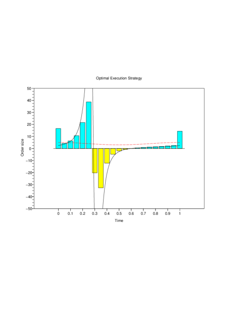
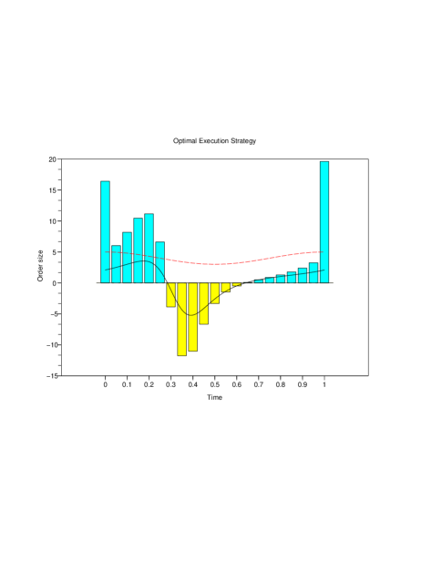
Figure 2: Optimal execution strategy to buy $50$ shares on a regular time grid, with $N=20$, $\rho=1$, $\lambda(t)=4+\cos(2\pi t)$ (plotted in dashed line) and $\gamma=-0.3$ (left) or $\gamma=1$ (right). In solid line is plotted the function $t\mapsto\left(\frac{\rho_{t}(1+\gamma)}{\rho_{t}(2+\gamma)+\eta_{t}}\right)^{\prime}+\rho_{t}\left(\frac{\rho_{t}+\eta_{t}}{\rho_{t}(2+\gamma)+\eta_{t}}\right)$ (this function is well-defined but out of the graph for $\gamma=-0.3$).

2.2.2 Price impact reversion model

The results that we present for model $P$ are similar to the one obtained for model $V$. We first solve the optimal execution problem in discrete time. From its explicit solution, we then calculate its continuous time limit and check by a verification argument that it is indeed optimal. Doing so, we get sufficient conditions to exclude PMS and TTPM. In particular, condition (30) that excludes PMS and TTPM for block-shape LOB also excludes PMS and TTPM for a general LOB shape satisfying Assumption 2.2 below.

To study the optimal discrete strategy, we will work under the following assumption.

Assumption 2.2.

1. The shape function $f$ is $\mathcal{C}^{1}$ and satisfies the following condition:

   $$f\text{ is nonincreasing on }\mathbb{R_{-}}\text{ and nondecreasing on }\mathbb{R_{+}}$$

2. $\forall t\geq 0,\rho_{t}-\eta_{t}>0$.

3. $x\mapsto x\frac{f^{\prime}(x)}{f(x)}$ is nondecreasing on $\mathbb{R}_{-}$, nonincreasing on $\mathbb{R}_{+}$.

The monotonicity assumption made here is the opposite to the one made in Assumption 2.1 for model $V$. This choice is different from the one made in Alfonsi et al. [2, 3]. It is in fact more tractable from a mathematical point of view, especially here with a time-varying LOB.

Theorem 2.5.

Under Assumption 2.2, the cost function $C^{P}({\bm{\xi}},{\bm{t}})$ is nonnegative, and there is a unique optimal execution strategy ${\bm{\xi}}^{\star}$ that minimizes $C^{P}$ over $\{{\bm{\xi}}\in\mathbb{R}^{N+1},\sum_{i=0}^{N}\xi_{i}=-\mathbbm{x}\}$. This strategy is given as follows. The following equation

$$\sum_{i=1}^{N}\lambda(t_{i-1})\left[F\left(\frac{h^{-1}_{P,i}(\nu)}{a_{i}}\right)-\frac{\lambda(t_{i})}{\lambda(t_{i-1})}F(h^{-1}_{P,i}(\nu))\right]+\lambda(t_{N})F(\nu)=-\mathbbm{x}$$

has a unique solution $\nu\in\mathbb{R}$, and

$$\xi^{\star}_{0} = \lambda(t_{0})F\left(\frac{h^{-1}_{P,1}\left(\nu\right)}{a_{1}}\right),$$

$$\xi^{\star}_{i} = \lambda(t_{i})\left[F\left(\frac{h^{-1}_{P,i+1}\left(\nu\right)}{a_{i+1}}\right)-F(h^{-1}_{P,i}(\nu))\right],\ 1\leq i\leq N-1,$$

$$\xi^{\star}_{N} = \lambda(t_{N})[F(\nu)-F(h^{-1}_{P,N}\left(\nu\right))].$$

The first and the last trade have the same sign as $-\mathbbm{x}$.

We now state the corresponding result in continuous time and set:

$$x\in\mathbb{R},\ h_{P,t}(x)=x\left[1+\frac{\rho_{t}}{\rho_{t}\left(1+\frac{xf^{\prime}(x)}{f(x)}\right)-\eta_{t}}\right].$$ (37)

Theorem 2.6.

Let $f\in\mathcal{C}^{2}(\mathbb{R})$. We assume that one of the two following conditions holds.

1. For $t\in[0,T]$, $\rho_{t}\left(1+\frac{xf^{\prime}(x)}{f(x)}\right)-\eta_{t}>0$ for any $x\in\mathbb{R}$ and $h_{P,t}$ is bijective on $\mathbb{R}$, such that $h_{P,t}^{\prime}(x)>0$, $dx$-a.e.

2. For $t\in[0,T]$, $\rho_{t}\left(1+\frac{xf^{\prime}(x)}{f(x)}\right)-\eta_{t}<0$ and $\rho_{t}\left(2+\frac{xf^{\prime}(x)}{f(x)}\right)-\eta_{t}>0$ for any $x\in\mathbb{R}$, and $h_{P,t}$ is bijective on $\mathbb{R}$, such that $h_{P,t}^{\prime}(x)<0$, $dx$-a.e.

Then, the cost function $C^{P}(X)$ is nonnegative, and there is a unique optimal admissible strategy $X^{\star}$ that minimizes $C^{P}$. This strategy is given as follows. The equation

$$\int_{0}^{T}\lambda(t)[\rho_{t}h_{P,t}^{-1}(\nu)f(h_{P,t}^{-1}(\nu))-\eta_{t}F(h_{P,t}^{-1}(\nu))]dt+\lambda(T)F(\nu)=-\mathbbm{x}$$ (38)

has a unique solution $\nu\in\mathbb{R}$ and we set $\zeta_{t}=h_{P,t}^{-1}(\nu)$. The strategy $dX^{\star}_{t}=\xi^{\star}_{0}\delta_{0}(dt)+\xi^{\star}_{t}dt+\xi^{\star}_{T}\delta_{T}(dt)$ with

$$\xi^{\star}_{0} = \lambda(0)F(\zeta_{0}),$$

$$\xi^{\star}_{t} = \lambda(t)f(\zeta_{t})\left[\frac{d\zeta_{t}}{dt}+\rho_{t}\zeta_{t}\right],$$

$$\xi^{\star}_{T} = \lambda(T)(F(\nu)-F(\zeta_{T})),$$

is optimal. The initial trade $\xi^{\star}_{0}$ has the same sign as $-\mathbbm{x}$.

In particular, there is no PMS in model $P$ as soon as Assumptions $(i)$ or $(ii)$ hold. Conversely, let us assume that $\rho_{t_{1}}\left(2+\frac{xf^{\prime}(x)}{f(x)}\right)-\eta_{t_{1}}<0,$ when $x$ belongs to a neighbourhood of $0$ for some $t_{1}\geq 0$. Then, we set ${\bf t}=(0,t_{1},t_{2})$ with $t_{2}>t_{1}$, and consider that the large trader buys $x>0$ at time $t_{1}$ and sells $x$ at time $t_{2}$. The cost of such a round trip is

$$C^{P}((0,x,-x),{\bm{t}})$$

$$= \lambda(t_{1})G\left(\frac{x}{\lambda(t_{1})}\right)+\lambda(t_{2})\left[G\left(F\left(e^{-\int_{t_{1}}^{t_{2}}\rho_{s}ds}F^{-1}\left(\frac{x}{\lambda(t_{2})}\right)\right)-\frac{x}{\lambda(t_{2})}\right)-\tilde{F}\left(e^{-\int_{t_{1}}^{t_{2}}\rho_{s}ds}F^{-1}\left(\frac{x}{\lambda(t_{2})}\right)\right)\right]$$

$$= \lambda(t_{1})\left[-\eta_{t_{1}}\tilde{F}\left(F^{-1}\left(\frac{x}{\lambda(t_{1})}\right)\right)+\rho_{t_{1}}F^{-1}\left(\frac{x}{\lambda(t_{1})}\right)^{2}f\left(F^{-1}\left(\frac{x}{\lambda(t_{1})}\right)\right)\right](t_{2}-t_{1})+o(t_{2}-t_{1}).$$

The derivative of $x\mapsto-\eta_{t_{1}}\tilde{F}(x)+\rho_{t_{1}}x^{2}f(x)$ is $xf(x)\left(\rho_{t_{1}}\left(2+\frac{xf^{\prime}(x)}{f(x)}\right)-\eta_{t_{1}}\right)$ and has the opposite sign of $x$ near $0$. Thus, $C^{P}((0,x,-x),{\bm{t}})$ is negative when $t_{2}$ is close to $t_{1}$ and $x$ is small enough, which gives a PMS.

Corollary 2.6.

Let $f\in\mathcal{C}^{2}(\mathbb{R})$. Under Assumption 2.2, the function $h_{P,t}$ is $\mathcal{C}^{1}(\mathbb{R})$, bijective on $\mathbb{R}$ and such that $h_{P,t}^{\prime}>0$. Thus, the result of Theorem 2.6 holds and the last trade $\xi^{\star}_{T}$ has the same sign as $-\mathbbm{x}$.

Besides, if (30) also holds, $\xi^{\star}_{t}$ has the same sign as $-\mathbbm{x}$ for any $0<t<T$, which rules out TTPM.

As for model $V$, we consider now the case of a power-law shape $f(x)=|x|^{\gamma}$. We can apply the results of Theorem 2.6 in this case. We can also notice from (9) that $dE_{t}=(\eta_{t}-\rho_{t}(1+\gamma))E_{t}dt$. Therefore, model $P$ with resilience $\rho_{t}$ is the same as model $V$ with resilience $\tilde{\rho}_{t}=\rho_{t}(1+\gamma)-\eta_{t}$.

Corollary 2.7.

When $f(x)=|x|^{\gamma}$, model $P$ does not admit PMS if, and only if

$$\forall t\geq 0,\ \rho_{t}(2+\gamma)-\eta_{t}\geq 0.$$

It does not admit transaction-triggered price manipulation if and only if

$$\forall t\geq 0,\ \rho_{t}(1+\gamma)-\eta_{t}\geq 0,\ \text{and }\left(\frac{\rho_{t}(1+\gamma)-\eta_{t}}{\rho_{t}(2+\gamma)-\eta_{t}}\right)^{\prime}+\rho_{t}\left(\frac{\rho_{t}(1+\gamma)-\eta_{t}}{\rho_{t}(2+\gamma)+\eta_{t}}\right)\geq 0.$$

3 Proofs

3.1 The block shape case

Proof of Theorem 2.1: The quadratic form (16) is given by $C^{V}({\bm{\xi}},{\bm{t}})=\frac{1}{2}{\bm{\xi}}^{T}M^{V}{\bm{\xi}}$, with $M^{V}_{i,j}=\frac{\exp\left(-\left|\int_{t_{i}}^{t_{j}}\rho_{s}ds\right|\right)}{\lambda(t_{i}\vee t_{j})}$, $0\leq i,j\leq N$. Let us assume that $a_{i}\tilde{a}_{i}<1,\forall i\in\left\{1,\ldots,N\right\}$. Then, we can define the following vectors:

$$\mathbf{y}_{0}=\frac{\mathbf{e}_{0}}{\sqrt{\lambda(t_{0})}},\ \mathbf{y}_{i}=\tilde{a}_{i}\mathbf{y}_{i-1}+\frac{\mathbf{e}_{i}}{\sqrt{\lambda(t_{i})}}\sqrt{1-a_{i}\tilde{a}_{i}},\ 1\leq i\leq N$$

where $\mathbf{e}_{0}\ldots\mathbf{e}_{N}$ denote the canonical basis of $\mathbb{R}^{N+1}$. We have $M^{V}_{ij}=\mathbf{y}_{i}^{T}\mathbf{y}_{j}$. We introduce $Y$ the upper triangular matrix with columns $\mathbf{y}_{0},\ldots,\mathbf{y}_{N}$. By assumption, it is invertible and so is $M=Y^{T}Y$. Conversely, if $M^{V}$ is positive definite, the minors

$$\det((M^{V}_{i,j})_{0\leq i,j\leq n})=\frac{1}{\lambda(t_{0})}\prod^{n}_{i=1}\frac{1}{\lambda(t_{i})}(1-a_{i}\tilde{a}_{i}),\ 1\leq n\leq N$$

are positive, which gives (17).

Let us turn to the optimization problem. One has to minimize $C^{V}({\bm{\xi}},{\bm{t}})$ under the linear constraint $\sum_{i=0}^{N}\xi_{i}=-\mathbbm{x}$, which gives

$${\bm{\xi}}^{\star}=-\frac{\mathbbm{x}}{\mathbf{1}^{T}\left(M^{V}\right)^{-1}\mathbf{1}}\left(M^{V}\right)^{-1}\mathbf{1},$$ (39)

where $\mathbf{1}\in\mathbb{R}^{N+1}$ is a vector of ones. Since $Y$ is upper triangular, it can be easily inverted and we can calculate explicitly $\left(M^{V}\right)^{-1}\mathbf{1}$ and get (18). $\Box$

3.2 General LOB shape with model $V$

Let us introduce some notations. For the time grid ${\bm{t}}$ given by (14), we introduce the next quantities:

$$\alpha_{k}:=\int^{t_{k}}_{t_{k-1}}\rho_{s}ds,\>k=1,\ldots,N.$$ (40)

We can write the cost function (13) as follows

$$C^{V}({\bm{\xi}},{\bm{t}})=\sum^{N}_{n=0}\lambda(t_{n})\left[G\left(\frac{E_{{n}}+\xi_{n}}{\lambda(t_{n})}\right)-G\left(\frac{E_{{n}}}{\lambda(t_{n})}\right)\right],$$ (41)

where we use the following notations (observe that $E_{n}=a_{n}(E_{n-1}+\xi_{n-1})$)

$$E_{0}=0,\ E_{n}=\sum^{n-1}_{i=0}\xi_{i}e^{-\sum^{n}_{k=i+1}\alpha_{k}},\>1\leq n\leq N.$$

Lemma 3.1.

We have $\frac{\partial C^{V}}{\partial\xi_{N}}=F^{-1}\left(\frac{E_{N}+\xi_{N}}{\lambda(t_{N})}\right)$ and, for $i=0,\ldots,N-1$,

$$\frac{\partial C^{V}}{\partial\xi_{i}}-a_{i+1}\frac{\partial C^{V}}{\partial\xi_{i+1}}=F^{-1}\left(\frac{E_{i}+\xi_{i}}{\lambda(t_{i})}\right)-a_{i+1}F^{-1}\left(\frac{E_{i+1}}{\lambda(t_{i+1})}\right).$$ (42)

Proof.

Let us first observe that $\frac{\partial E_{n}}{\partial\xi_{i}}=0,\>\text{ if }i\geq n,\>\text{and }\frac{\partial E_{n}}{\partial\xi_{i}}=e^{-\sum^{n}_{k=i+1}\alpha_{k}}\>\text{ if }i<n$. Thus, we get by using that $G^{\prime}=F^{-1}$:

$$\frac{\partial C^{V}}{\partial\xi_{i}} = F^{-1}\left(\frac{E_{i}+\xi_{i}}{\lambda(t_{i})}\right)+\sum^{N}_{n=i+1}e^{-\sum^{n}_{k=i+1}\alpha_{k}}\left(F^{-1}\left(\frac{E_{n}+\xi_{n}}{\lambda(t_{n})}\right)-F^{-1}\left(\frac{E_{n}}{\lambda(t_{n})}\right)\right)$$

$$= F^{-1}\left(\frac{E_{i}+\xi_{i}}{\lambda(t_{i})}\right)-e^{-\alpha_{i+1}}F^{-1}\left(\frac{E_{i+1}}{\lambda(t_{i+1})}\right)$$

$$+ e^{-\alpha_{i+1}}\left[F^{-1}\left(\frac{E_{i+1}+\xi_{i+1}}{\lambda(t_{i+1})}\right)+\sum^{N}_{n=i+2}e^{-\sum^{n}_{k=i+2}\alpha_{k}}\left(F^{-1}\left(\frac{E_{n}+\xi_{n}}{\lambda(t_{n})}\right)-F^{-1}\left(\frac{E_{n}}{\lambda(t_{n})}\right)\right)\right]$$

$$= F^{-1}\left(\frac{E_{i}+\xi_{i}}{\lambda(t_{i})}\right)-a_{i+1}F^{-1}\left(\frac{E_{i+1}}{\lambda(t_{i+1})}\right)+a_{i+1}\frac{\partial C^{V}}{\partial\xi_{i+1}}.$$

∎

Lemma 3.2.

Under Assumption 2.1, we obtain the next conclusions.

1. For $i\in\left\{1,\ldots,N\right\}$, the function $h_{V,i}$ defined in (32) is an increasing bijection on $\mathbb{R}$ that satisfies $\mathrm{sgn}(x)h_{V,i}(x)\geq\frac{1-a_{i}\tilde{a}_{i}}{1-a_{i}}F^{-1}(x)$.

2. If (33) holds, then we have $\mathrm{sgn}(x)h^{-1}_{V,i+1}\left(x\right)\geq\mathrm{sgn}(x)\tilde{a}_{i}h^{-1}_{V,i}\left(x\right)$ for $i\in\left\{1,\ldots,N-1\right\}$.

3. $\mathrm{sgn}(x)F(x)\geq\mathrm{sgn}(x)\tilde{a}_{N}h^{-1}_{V,N}\left(x\right)$.

Proof.

1. Since the resilience $\rho_{t}$ is positive, we have $0<a_{i}<1$, and $\tilde{a}_{i}\leq 1$ since $\rho_{t}+\eta_{t}\geq 0$ by Assumption 2.1. We then get

   $$\frac{\partial h_{V,i}(x)}{\partial x}=\frac{1}{1-a_{i}}\left[\frac{1}{f(F^{-1}(x))}-\frac{a_{i}\tilde{a}_{i}}{f(F^{-1}(\tilde{a}_{i}x))}\right]\geq\frac{1-a_{i}\tilde{a}_{i}}{1-a_{i}}\frac{1}{f(F^{-1}(x))}>0$$

   because $f$ is nondecreasing on $\mathbb{R_{-}}$ and nonincreasing on $\mathbb{R_{+}}$, and $F^{-1}$ is increasing.

2. We set $\hat{f}(x)=(F^{-1})^{\prime}(x)=1/f(F^{-1}(x))$: this function is positive, nonincreasing on $\mathbb{R}_{-}$ and nondecreasing on $\mathbb{R}_{+}$. Let $\nu\geq 0$ and $y=h^{-1}_{V,i+1}(\nu)$. We note that $y\geq 0$ because $h_{V,i+1}(0)=0$ and $h_{V,i+1}$ is increasing by the first point of this lemma. Thus, we have that

   $$\nu = \frac{F^{-1}(y)-a_{i+1}F^{-1}(\tilde{a}_{i+1}y)}{1-a_{i+1}}$$

   $$= F^{-1}(\tilde{a}_{i+1}y)+\frac{F^{-1}(y)-F^{-1}(\tilde{a}_{i+1}y)}{1-a_{i+1}}$$

   $$= F^{-1}(\tilde{a}_{i+1}y)+\frac{1}{1-a_{i+1}}\int^{y}_{\tilde{a}_{i+1}y}\hat{f}(\xi)d\xi\leq F^{-1}(y)+\frac{1-\tilde{a}_{i+1}}{1-a_{i+1}}y\hat{f}(y)=:g_{i+1}(y)$$

   Hence, we obtain that $g_{i+1}$ is increasing on $\mathbb{R}$ and then, $y\geq g^{-1}_{i+1}(\nu)$. Let $z=\tilde{a}_{i}h^{-1}_{V,i}\left(\nu\right)\geq 0$. We have:

   $$\nu = \frac{F^{-1}\left(\frac{z}{\tilde{a}_{i}}\right)-a_{i}F^{-1}(z)}{1-a_{i}}$$

   $$= F^{-1}(z)+\frac{F^{-1}\left(\frac{z}{\tilde{a}_{i}}\right)-F^{-1}(z)}{1-a_{i}}$$

   $$= F^{-1}(z)+\frac{1}{1-a_{i}}\int^{\frac{z}{\tilde{a}_{i}}}_{z}\hat{f}(\xi)d\xi\geq F^{-1}(z)+\frac{\left(\frac{1}{\tilde{a}_{i}}-1\right)}{1-a_{i}}z\hat{f}(z)=:\bar{g}_{i}(z)$$

   Therefore, if (33) holds, we get that $g_{i+1}(x)\leq\bar{g}_{i}(x)$ for all $x\geq 0$. Then, we have $g^{-1}_{i+1}(x)\geq g^{-1}_{i}(x)$, and therefore

   $$y\geq g^{-1}_{i+1}(\nu)\geq g^{-1}_{i}(\nu)\geq z.$$

   The same arguments for $\nu\leq 0$ give $y\leq g^{-1}_{i+1}(\nu)\leq g^{-1}_{i}(\nu)\leq z$.

3. Using the above definition, we have $\mathrm{sgn}(x)\bar{g}_{N}(x)\geq\mathrm{sgn}(x)F^{-1}(x)$, and therefore we get

   $$\mathrm{sgn}(\nu)F(\nu)\geq\mathrm{sgn}(\nu)\bar{g}^{-1}_{N}(\nu)\geq\mathrm{sgn}(\nu)z=\mathrm{sgn}(\nu)\tilde{a}_{N}h^{-1}_{V,N}\left(\nu\right).$$

∎

Lemma 3.3.

Let $a\in(0,1)$ and $b>0$ such that $ab\leq 1$. We have $G(x)-\frac{1}{b}G(abx)\geq 0$ for $x\in\mathbb{R}$, and $G(x)-\frac{1}{b}G(abx)\underset{|x|\rightarrow+\infty}{\rightarrow}+\infty$.

Proof.

Since $G$ is convex ($G^{\prime}=F^{-1}$ is increasing) and $G(0)=0$, $G(abx)\leq abG(x)$. If $b>1$, we then have $G(x)-\frac{1}{b}G(abx)\geq G(x)(1-a)$ which gives the result. If $b\leq 1$, we have

$$G(x)-\frac{1}{b}G(abx) = \int^{x}_{0}F^{-1}(u)du-\frac{1}{b}\int^{abx}_{0}F^{-1}(u)du=\int^{x}_{0}F^{-1}(u)du-\int^{ax}_{0}F^{-1}(bv)dv$$

$$= \int^{x}_{ax}F^{-1}(u)du+\int^{ax}_{0}\left(F^{-1}(u)-F^{-1}(bu)\right)du\geq|x|(1-a)F^{-1}(|ax|)\underset{|x|\rightarrow+\infty}{\rightarrow}\infty.\qed$$

Proof of Theorem 2.3: We rewrite the cost function (41) to minimize as follows:

$$C^{V}({\bm{\xi}},{\bm{t}}) = \sum^{N}_{n=0}\lambda(t_{n})\left[G\left(\frac{E_{n}+\xi_{n}}{\lambda(t_{n})}\right)-G\left(\frac{E_{n}}{\lambda(t_{n})}\right)\right]$$

$$= \lambda(t_{N})G\left(\frac{\sum^{N}_{i=0}\xi_{i}e^{-\sum^{N}_{k=i+1}\alpha_{k}}}{\lambda(t_{N})}\right)-\lambda(0)G(0)$$

$$+ \sum^{N-1}_{n=0}\left[\lambda(t_{n})G\left(\frac{\sum^{n}_{i=0}\xi_{i}e^{-\sum^{n}_{k=i+1}\alpha_{k}}}{\lambda(t_{n})}\right)-\lambda(t_{n+1})G\left(\frac{e^{-\alpha_{n+1}}\sum^{n}_{i=0}\xi_{i}e^{-\sum^{n}_{k=i+1}\alpha_{k}}}{\lambda(t_{n+1})}\right)\right]$$

We define the linear map $T:\mathbb{R}^{N+1}\rightarrow\mathbb{R}^{N+1}$ by $(T\xi)_{n}=\frac{\sum^{n}_{i=0}\xi_{i}e^{-\sum^{n}_{k=i+1}\alpha_{k}}}{\lambda(t_{n})}$, so that

$$C^{V}({\bm{\xi}},{\bm{t}})=\lambda(t_{N})G((T\xi)_{N})+\sum^{N-1}_{n=0}\left[\lambda(t_{n})G((T\xi)_{n})-\lambda(t_{n+1})G\left(\tilde{a}_{n+1}(T\xi)_{n}\right)\right].$$ (43)

Let us observe that $T$ is a linear bijection. By Lemma 3.3 we get that $C^{V}({\bm{\xi}},{\bm{t}})\geq 0$ and $C^{V}({\bm{\xi}},{\bm{t}})\underset{|{\bm{\xi}}|\rightarrow+\infty}{\rightarrow}+\infty$, which gives the existence of a minimizer ${\bm{\xi}}^{\star}$ over ${\bm{\xi}}$, s.t. $\sum_{i=0}^{N}\xi_{i}=-\mathbbm{x}$. Thus, by using (42), there must be a Lagrange multiplier $\nu$ such that

$$\nu=h_{V,i+1}\left(\frac{E_{i}+\xi^{\star}_{i}}{\lambda(t_{i})}\right),\>i=0\ldots N-1,\text{ and }\nu=F^{-1}\left(\frac{E_{N}+\xi^{\star}_{N}}{\lambda(t_{N})}\right).$$ (44)

We have $\frac{E_{i}+\xi^{\star}_{i}}{\lambda(t_{i})}=h^{-1}_{V,i+1}\left(\nu\right)$ and then $E_{i+1}=\lambda(t_{i})a_{i+1}h^{-1}_{V,i+1}\left(\nu\right)$, for $0\leq i\leq N-1$. Thus, we get

$$\xi^{\star}_{0} = \lambda(t_{0})h^{-1}_{V,1}\left(\nu\right),$$

$$\xi^{\star}_{i} = \lambda(t_{i})h^{-1}_{V,i+1}\left(\nu\right)-\lambda(t_{i-1})a_{i}h^{-1}_{V,i}\left(\nu\right),\ 1\leq i\leq N-1,$$

$$\xi^{\star}_{N} = F(\nu)\lambda(t_{N})-\lambda(t_{N-1})a_{N}h^{-1}_{V,N}\left(\nu\right)$$

Furthermore, we note that

$$\sum^{N}_{i=0}\xi^{\star}_{i}=-\mathbbm{x}=\lambda(t_{0})(1-a_{1})h^{-1}_{V,1}(\nu)+\ldots+\lambda(t_{N-1})(1-a_{N})h^{-1}_{V,N}(\nu)+F(\nu)\lambda(t_{N}).$$

By Lemma 3.2 The right side is an increasing bijection on $\mathbb{R}$, and we deduce that there is only one $\nu\in\mathbb{R}$ which satisfies the above equation. This give the uniqueness of the minimizer ${\bm{\xi}}^{\star}$. Moreover, the functions $F^{-1}$ and $h_{V,i}$ vanish in $0$, and $\nu$ has the same sign as $-\mathbbm{x}$, which gives that $\xi^{\star}_{0}$ and $\xi^{\star}_{N}$ have the same sign as $-\mathbbm{x}$ by Lemma 3.2. Besides, if (33) holds, the trades $\xi^{\star}_{i}$ have also the same sign as $-\mathbbm{x}$. $\Box$

Let us now prepare the proof of Theorem 2.4 and assume that $h_{V,t}$ is bijective increasing. We introduce for $0\leq t\leq T$,

$$C^{V}(t,T,E_{t},X_{t})=\lambda(t)\left[G(\zeta_{t})-G\left(\frac{E_{t}}{\lambda(t)}\right)\right]+\int_{t}^{T}F^{-1}(\zeta_{u})\xi_{u}du+\lambda(T)[G(F(\nu))-G(\zeta_{T})],$$ (45)

where

$$\nu\in\mathbb{R},s.t.-E_{t}+\int_{t}^{T}\lambda(u)\rho_{u}h_{V,u}^{-1}(\nu)du+\lambda(T)F(\nu)=-X_{t},$$ (46)

$$\zeta_{u}=h_{V,u}^{-1}(\nu),\ \xi_{u}=\lambda(u)[\frac{d\zeta_{u}}{du}+(\rho_{u}+\eta_{u})\zeta_{u}].$$ (47)

Let us observe that $\nu\mapsto\int_{t}^{T}\lambda(u)\rho_{u}h_{V,u}^{-1}(\nu)du+\lambda(T)F(\nu)$ is increasing an bijective on $\mathbb{R}$, and (46) admits a unique solution. The function $C^{V}(t,T,E_{t},X_{t})$ denotes the minimal cost to liquidate $X_{t}$ shares on the time interval $[t,T]$ given the current state $E_{t}$. In particular, we observe that

$$C^{V}(T,T,E_{T},X_{T})=\lambda(T)\left[G\left(\frac{E_{T}-X_{T}}{\lambda(T)}\right)-G\left(\frac{E_{T}}{\lambda(T)}\right)\right],$$

which is the cost of selling $X_{T}$ shares at time $T$. Besides, an integration by parts gives that

$$C^{V}(t,T,E_{t},X_{t})=-\lambda(t)G\left(\frac{E_{t}}{\lambda(t)}\right)+\int_{t}^{T}\lambda(u)\left[(\rho_{u}+\eta_{u})F^{-1}(\zeta_{u})\zeta_{u}-\eta_{u}G(\zeta_{u})\right]du+\lambda(T)G(F(\nu)).$$ (48)

The function $\zeta\mapsto(\rho_{u}+\eta_{u})F^{-1}(\zeta)\zeta-\eta_{u}G(\zeta)$ is nonnegative since it vanishes at $0$, and its derivative is equal to $\rho_{u}h_{V,u}(\zeta)$ that has the same sign as $\zeta$. Since $G\geq 0$, we get:

$$C^{V}(0,T,0,\mathbbm{x})\geq 0.$$ (49)

Formula (45) can be guessed by simple but tedious calculations: one has to consider the associated discrete problem on a regular time-grid and then let the time-step going to zero. We do not present these calculations here since we will prove directly by a verification argument that this is indeed the minimal cost.

Proof of Theorem 2.4: Let $(X_{t},0\leq t\leq T+)$ denote an admissible strategy that liquidates $\mathbbm{x}$. We consider $(E_{t},0\leq t\leq T+)$ the solution of $dE_{t}=dX_{t}-\rho_{t}E_{t}dt$, $\nu_{t}$ the solution of (46) and $\zeta_{t}=h_{V,t}^{-1}(\nu_{t})$. We set

$$C_{t}=\int_{0}^{t}F^{-1}\left(\frac{E_{s}}{\lambda(s)}\right)dX^{c}_{s}+\sum_{0\leq s<t}\lambda(s)\left[G\left(\frac{E_{s}+\Delta X_{s}}{\lambda(s)}\right)-G\left(\frac{E_{s}}{\lambda(s)}\right)\right]+C^{V}(t,T,E_{t},X_{t}).$$

Let us observe that $C_{T}=C^{V}(X)$ and $C_{0}=C^{V}(0,T,0,\mathbbm{x})$. We are going to show that $dC_{t}\geq 0$, and that $dC_{t}=0$ holds only for $X^{\star}$. This will in particular show that $C^{V}(X)\geq 0$ from (49).

Let us first consider the case of a jump $\Delta X_{t}>0$. Then, we have

$$\Delta C_{t}=\lambda(t)\left[G\left(\frac{E_{t}+\Delta X_{t}}{\lambda(t)}\right)-G\left(\frac{E_{t}}{\lambda(t)}\right)\right]+C^{V}(t+,T,E_{t+},X_{t+})-C^{V}(t,T,E_{t},X_{t}).$$

Since $\Delta E_{t}=\Delta X_{t}$, the solution $\nu_{t}$ of (46) is also the solution of $-E_{t+}+\int_{t}^{T}\lambda(u)\rho_{u}h_{V,u}^{-1}(\nu_{t})du+\lambda(T)F(\nu_{t})=-X_{t+}$, and then $\Delta C_{t}=0$. Now, let us calculate $dC_{t}$. We set

$$\tilde{C}(t,T,E_{t},X_{t},v) = \lambda(T)G(F(v))-\lambda(t)G\left(\frac{E_{t}}{\lambda(t)}\right)$$

$$+\int_{t}^{T}\lambda(u)\left[(\rho_{u}+\eta_{u})F^{-1}(h_{V,u}^{-1}(v))h_{V,u}^{-1}(v)-\eta_{u}G(h_{V,u}^{-1}(v))\right]du.$$

Then, we have from (48):

$$dC_{t} = F^{-1}\left(\frac{E_{t}}{\lambda(t)}\right)dX^{c}_{t}-\lambda^{\prime}(t)G\left(\frac{E_{t}}{\lambda(t)}\right)dt-F^{-1}\left(\frac{E_{t}}{\lambda(t)}\right)(dX^{c}_{t}-(\rho_{t}+\eta_{t})E_{t}dt)$$

$$-\lambda(t)(\rho_{t}+\eta_{t})F^{-1}(\zeta_{t})\zeta_{t}dt+\lambda^{\prime}(t)G(\zeta_{t})dt+\frac{\partial\tilde{C}}{\partial v}(t,T,E_{t},X_{t},\nu_{t})d\nu_{t}.$$

Since $\left[\lambda(T)f(\nu_{t})+\int_{t}^{T}\lambda(u)\rho_{u}(h_{V,u}^{-1})^{\prime}(\nu_{t})du\right]d\nu_{t}-\lambda(t)\rho_{t}h_{V,t}^{-1}(\nu_{t})dt=d(E_{t}-X_{t})=-\rho_{t}E_{t}dt$ and

$$\partial_{v}\tilde{C}(t,T,E_{t},X_{t},v) = \lambda(T)vf(v)+\int_{t}^{T}\lambda(u)\rho_{u}(h_{V,u}^{-1})^{\prime}(v)\left[F^{-1}(h_{V,u}^{-1}(v))+\frac{\rho_{u}+\eta_{u}}{\rho_{u}}\frac{h_{V,u}^{-1}(v)}{f(h_{V,u}^{-1}(v))}\right]du$$

$$= v\left[\lambda(T)f(v)+\int_{t}^{T}\lambda(u)\rho_{u}(h_{V,u}^{-1})^{\prime}(v)du\right],$$

we finally get

$$dC_{t} = \lambda(t)\left[(\rho_{t}+\eta_{t})\left(\frac{E_{t}}{\lambda(t)}F^{-1}\left(\frac{E_{t}}{\lambda(t)}\right)-\zeta_{t}F^{-1}(\zeta_{t})\right)+\eta_{t}\left(G(\zeta_{t})-G\left(\frac{E_{t}}{\lambda(t)}\right)\right)+\rho_{t}h_{V,t}(\zeta_{t})\left(\zeta_{t}-\frac{E_{t}}{\lambda(t)}\right)\right]dt$$ (50)

$$:= \lambda(t)\psi_{t}(\zeta_{t})dt.$$

We have $\psi_{t}^{\prime}(\zeta)=-(\rho_{t}+\eta_{t})\left(F^{-1}(\zeta)+\frac{\zeta}{f(F^{-1}(\zeta))}\right)+\eta_{t}F^{-1}(\zeta)+\rho_{t}h_{V,t}(\zeta)+\rho_{t}h_{V,t}^{\prime}(\zeta)(\zeta-\frac{E_{t}}{\lambda(t)})=\rho_{t}h_{V,t}^{\prime}(\zeta)(\zeta-\frac{E_{t}}{\lambda(t)})$. Since $h_{V,t}^{\prime}>0$, $\psi_{t}$ vanishes at $\zeta=\frac{E_{t}}{\lambda(t)}$, and is positive for $\zeta\not=\frac{E_{t}}{\lambda(t)}$.

Thus, if $X$ is an optimal strategy, we necessarily have $\zeta_{t}=\frac{E_{t}}{\lambda(t)}$, $dt$-a.e. Then, we get by differentiating $\left[X_{t}-E_{t}+\int_{t}^{T}\lambda(u)\rho_{u}h_{V,u}^{-1}(\nu_{t})du+\lambda(T)F(\nu_{t})\right]=0$ that $\left[\int_{t}^{T}\lambda(u)\rho_{u}(h_{V,u}^{-1})^{\prime}(\nu_{t})du+\lambda(T)f(\nu_{t})\right]d\nu_{t}=0,$ which gives $d\nu_{t}=0$ since $(h_{V,u}^{-1})^{\prime}>0$ and $f>0$. Thus, we get that $\nu_{t}=\nu$ where $\nu$ is the solution of (35). In particular, we get $\Delta X_{0}=E_{0+}=\lambda(0)h_{V,0}^{-1}(0)=\Delta X^{\star}_{0}$ and then $X=X^{\star}$, which gives the uniqueness of the optimal strategy. Last we observe that $\nu$ has the same sign as $-\mathbbm{x}$ and thus $\xi^{\star}_{0}$ has the same sign as $-\mathbbm{x}$. $\Box$

Proof of Corollary 2.4: Since $\rho_{t}+\eta_{t}\geq 0$ and $xf^{\prime}(F^{-1}(x))\geq 0$ by Assumption 2.1, we have

$$h^{\prime}_{V,t}(x)=\frac{\eta_{t}+2\rho_{t}}{\rho_{t}}\frac{1}{f(F^{-1}(x))}-\frac{\eta_{t}+\rho_{t}}{\rho_{t}}\frac{xf^{\prime}(F^{-1}(x))}{f(F^{-1}(x))^{3}}>0.$$

Also, we have $\mathrm{sgn}(x)h_{V,t}(x)\geq\mathrm{sgn}(x)F^{-1}(x)$ and then $\mathrm{sgn}(x)h_{V,t}^{-1}(x)\leq\mathrm{sgn}(x)F(x)$, which gives that the last trade $\xi^{\star}_{T}$ has the same sign as $-\mathbbm{x}$. Then, we have $\frac{d\zeta_{t}}{dt}=-\frac{1}{h_{V,t}^{\prime}(\zeta_{t})}\frac{dh_{V,t}}{dt}(\zeta_{t})$ and thus

$$\xi^{\star}_{t} = \frac{\lambda(t)\zeta_{t}}{h_{V,t}^{\prime}(\zeta_{t})}\left[-\frac{d\left(\eta_{t}/\rho_{t}\right)}{dt}\frac{1}{f(F^{-1}(\zeta_{t}))}+(\rho_{t}+\eta_{t})h_{V,t}^{\prime}(\zeta_{t})\right]$$

$$= \frac{\lambda(t)\zeta_{t}}{h_{V,t}^{\prime}(\zeta_{t})}\left[\frac{1}{\rho_{t}f(F^{-1}(\zeta_{t}))}\left(\frac{\rho_{t}^{\prime}\eta_{t}-\rho_{t}\eta_{t}^{\prime}}{\rho_{t}}+(\rho_{t}+\eta_{t})(2\rho_{t}+\eta_{t})\right)-\frac{(\eta_{t}+\rho_{t})^{2}}{\rho_{t}}\frac{\zeta_{t}f^{\prime}(\zeta_{t})}{f(F^{-1}(\zeta_{t}))^{3}}\right]$$

is nonnegative if (22) holds since $h_{V,t}^{\prime}>0$ and $\zeta_{t}f^{\prime}(\zeta_{t})\geq 0$. $\Box$

Lemma 3.4.

We have $\eqref{eq:condit_manip_price_vol_mod}\implies\eqref{eq:condit_t_t_manip_m_v}$ if $\rho_{t}+\eta_{t}\geq 0,\ t\geq 0$.

Proof.

We have

$$\eqref{eq:condit_manip_price_vol_mod}\Leftrightarrow\frac{1}{\tilde{a}_{i}}\frac{1-\tilde{a}_{i}}{1-a_{i}}\geq\frac{1-\tilde{a}_{i+1}}{1-a_{i+1}} \Leftrightarrow \left(1-a_{i+1}\right)-\tilde{a}_{i}\left(1-a_{i+1}\right)\geq\tilde{a}_{i}\left(1-a_{i}\right)-\tilde{a}_{i}\tilde{a}_{i+1}\left(1-a_{i}\right)$$

$$\Leftrightarrow \tilde{a}_{i+1}\left(1-a_{i}\right)+\frac{1}{\tilde{a}_{i}}(1-a_{i+1})\geq 1-a_{i}+1-a_{i+1}.$$

Since $\tilde{a}_{i+1}\leq 1$, we get $1-a_{i}+1-a_{i+1}=1-a_{i}a_{i+1}+(1-a_{i})(1-a_{i+1})\geq 1-a_{i}a_{i+1}+\tilde{a}_{i+1}(1-a_{i})(1-a_{i+1})$. Thus, $\eqref{eq:condit_manip_price_vol_mod}$ implies that:

$$\tilde{a}_{i+1}\left(1-a_{i}\right)+\frac{1}{\tilde{a}_{i}}(1-a_{i+1})\geq 1-a_{i}a_{i+1}+\tilde{a}_{i+1}(1-a_{i})(1-a_{i+1})$$

$$\Leftrightarrow 1-\tilde{a}_{i}+a_{i}a_{i+1}\tilde{a}_{i}-a_{i}\tilde{a}_{i+1}\geq a_{i+1}-\tilde{a}_{i}\tilde{a}_{i+1}a_{i+1}+a_{i}\tilde{a}_{i}a_{i+1}\tilde{a}_{i+1}-\tilde{a}_{i+1}a_{i+1}$$

$$\Leftrightarrow\left(1-\tilde{a}_{i}\right)\left(1-a_{i+1}\tilde{a}_{i+1}\right)\geq a_{i+1}\left(1-\tilde{a}_{i+1}\right)\left(1-a_{i}\tilde{a}_{i}\right)\Leftrightarrow\eqref{eq:condit_t_t_manip_m_v}.\qed$$

3.3 General LOB shape with model $P$

We first focus on discrete strategies on the time grid ${\bm{t}}$ such as (14). We introduce the following shorthand notation $D_{n}=D_{t_{n}}$ for $0\leq n\leq N$ and have

$$D_{0}=0,\ D_{n}=a_{n}F^{-1}\left(\frac{\xi_{n-1}}{\lambda(t_{n-1})}+F(D_{n-1})\right),\ 1\leq n\leq N.$$

We can write the cost function (13) as follows:

$$C^{P}({\bm{\xi}},{\bm{t}})=\sum^{N}_{n=0}\lambda(t_{n})\int^{D_{t_{n}+}}_{D_{t_{n}}}xf(x)dx=\sum^{N}_{n=0}\lambda(t_{n})\left[G\left(\frac{\lambda(t_{n})F(D_{n})+\xi_{n}}{\lambda(t_{n})}\right)-G(F(D_{n}))\right].$$ (51)

We begin with the following lemmas that we use to characterize the critical points of the optimization problem.

Lemma 3.5.

For $i=0,\ldots,N-1$, we have the following equations:

$$\frac{\partial C^{P}}{\partial\xi_{i}}=F^{-1}\left(\frac{\xi_{i}}{\lambda(t_{i})}+F(D_{i})\right)+\hat{a}_{i+1}\frac{f(D_{i+1})}{f\left(F^{-1}\left(\frac{\xi_{i}}{\lambda(t_{i})}+F(D_{i})\right)\right)}\left(\frac{\partial C^{P}}{\partial\xi_{i+1}}-D_{i+1}\right).$$

Proof.

First, we have $\frac{\partial D_{n}}{\partial\xi_{i}}=0$ for $i\geq n$, and the following recursive equations:

$$\frac{\partial D_{n}}{\partial\xi_{n-1}}=\frac{a_{n}}{\lambda(t_{n-1})f\left(F^{-1}(\frac{\xi_{n-1}}{\lambda(t_{n-1})}+F(D_{n-1}))\right)},\ \frac{\partial D_{n}}{\partial\xi_{i}}=\frac{\hat{a}_{i+1}f(D_{i+1})}{f\left(F^{-1}(\frac{\xi_{i}}{\lambda(t_{i})}+F(D_{i}))\right)}\frac{\partial D_{n}}{\partial\xi_{i+1}}\text{ for }1\leq i\leq n-2.$$

From (51), we get:

$$\frac{\partial C^{P}}{\partial\xi_{i}} = F^{-1}\left(\frac{\xi_{i}}{\lambda(t_{i})}+F(D_{i})\right)+\sum^{N}_{n=i+1}\left[F^{-1}\left(F(D_{n})+\frac{\xi_{n}}{\lambda(t_{n})}\right)-D_{n}\right]f(D_{n})\frac{\partial D_{n}}{\partial\xi_{i}}$$

$$= F^{-1}\left(\frac{\xi_{i}}{\lambda(t_{i})}+F(D_{i})\right)+\frac{\hat{a}_{i+1}f(D_{i+1})}{f\left(F^{-1}(\frac{\xi_{i}}{\lambda(t_{i})}+F(D_{i}))\right)}\left[F^{-1}(F(D_{i+1})+\frac{\xi_{i+1}}{\lambda(t_{i+1})})-D_{i+1}\right]$$

$$+\frac{\hat{a}_{i+1}f(D_{i+1})}{f\left(F^{-1}(\frac{\xi_{i}}{\lambda(t_{i})}+F(D_{i}))\right)}\left[\frac{\partial C^{P}}{\partial\xi_{i+1}}-F^{-1}\left(\frac{\xi_{i+1}}{\lambda(t_{i+1})}+F(D_{i+1})\right)\right],$$

which gives the result. ∎

Lemma 3.6.

Under Assumption 2.2, we have that:

1. The function $x\mapsto xf(x)$ is increasing on $\mathbb{R}$ (or equivalently, $\tilde{F}$ is convex).

2. We have $f\left(\frac{x}{a_{i}}\right)-\hat{a}_{i}f(x)>0,\;\;i=1,\ldots,N.$

3. The function

   $$x\in\mathbb{R},\ h_{P,i}(x)=x\frac{\left[\frac{1}{a_{i}}f(\frac{x}{a_{i}})-\hat{a}_{i}f(x)\right]}{f\left(\frac{x}{a_{i}}\right)-\hat{a}_{i}f(x)}$$

   is well-defined, bijective increasing and satisfies $\mathrm{sgn}(x)h_{P,i}(x)\geq|x|.$

Proof.

1. We have $\left(xf(x)\right)^{\prime}>0$ since $xf^{\prime}(x)\geq 0$ by Assumption 2.2.
2. We have for $x\in\mathbb{R}$,

$$\lambda(t_{i-1})f(\frac{x}{a_{i}})-\lambda(t_{i})a_{i}f(x)\geq\lambda(t_{i-1})f(x)(1-\hat{a}_{i})>0$$

because $f\left(\frac{x}{a_{i}}\right)\geq f(x)$ and $\hat{a}_{i}<1$ by Assumption 2.2.
3. The function $h_{P,i}$ is well-defined thanks to the second point. We have $\mathrm{sgn}(x)h_{P,i}(x)\geq|x|$ since

$$h_{P,i}(x)=x\left[1+\frac{a^{-1}_{i}}{1-\hat{a}_{i}\frac{f(x)}{f(\frac{x}{a_{i}})}}\right],$$

and it is sufficient to check that $f(x)/f(x/a_{i})$ is nondecreasing on $\mathbb{R}_{+}$ and nonincreasing on $\mathbb{R}_{-}$. We calculate

$$\left(\frac{f(x)}{f\left(\frac{x}{a_{i}}\right)}\right)^{\prime}=\frac{f^{\prime}(x)f\left(\frac{x}{a_{i}}\right)-\frac{1}{a_{i}}f(x)f^{\prime}\left(\frac{x}{a_{i}}\right)}{f\left(\frac{x}{a_{i}}\right)^{2}}.$$

This is nonnegative on $\mathbb{R}_{+}$ and nonpositive on $\mathbb{R}_{-}$ if and only if $\frac{xf^{\prime}(x)}{f(x)}\geq\frac{xf^{\prime}(x/a_{i})}{a_{i}f(x/a_{i})}$ for $x\in\mathbb{R}$, which holds by Assumption 2.2 since $|x|\leq|x|/a_{i}$. ∎

Proof of Theorem 2.5: We remark that the cost (51) can be written as follows:

$$C^{P}({\bm{\xi}},{\bm{t}}) = \lambda(t_{N})\tilde{F}\left(F^{-1}\left(F(D_{N})+\frac{\xi_{N}}{\lambda(t_{N})}\right)\right)$$

$$+ \sum^{N-1}_{n=0}\lambda(t_{n})\left[\tilde{F}\left(F^{-1}\left(F(D_{n})+\frac{\xi_{n}}{\lambda(t_{n})}\right)\right)-\frac{\lambda(t_{n+1})}{\lambda(t_{n})}\tilde{F}\left(a_{n+1}F^{-1}\left(F(D_{n})+\frac{\xi_{n}}{\lambda(t_{n})}\right)\right)\right].$$

Since $\tilde{F}$ is convex by Lemma 3.6 and $\tilde{F}(0)=0$, we have $\tilde{F}\left(a_{n+1}x\right)\leq a_{n+1}\tilde{F}(x)$, for $x\in\mathbb{R}$ and thus

$$C^{P}({\bm{\xi}},{\bm{t}}) \geq \lambda(t_{N})\tilde{F}\left(F^{-1}\left(F(D_{N})+\frac{\xi_{N}}{\lambda(t_{N})}\right)\right)+\sum^{N-1}_{n=0}\lambda(t_{n})\tilde{F}\left(F^{-1}\left(F(D_{n})+\frac{\xi_{n}}{\lambda(t_{n})}\right)\right)(1-\hat{a}_{n+1}).$$

In particular $C^{P}({\bm{\xi}},{\bm{t}})\geq 0$, since $\tilde{F}\geq 0$ and $\hat{a}_{n+1}<1$ by Assumption (2.2). Besides, by setting $T({\bm{\xi}})=\left(\frac{\xi_{0}}{\lambda(t_{0})},D_{1}+\frac{\xi_{1}}{\lambda(t_{1})},\dots,D_{N}+\frac{\xi_{N}}{\lambda(t_{N})}\right)$, we can easily check that $|T({\bm{\xi}})|\underset{|{\bm{\xi}}|\rightarrow+\infty}{\rightarrow}+\infty$, which gives immediately that $C^{P}({\bm{\xi}},{\bm{t}})\underset{|{\bm{\xi}}|\rightarrow+\infty}{\rightarrow}+\infty$ since $\tilde{F}(x)\underset{|x|\rightarrow+\infty}{\rightarrow}+\infty$.

Thus, there must be at least one minimizer of $C^{P}({\bm{\xi}},{\bm{t}})$ on $\{{\bm{\xi}}\in\mathbb{R}^{N+1},\sum_{i=0}^{N}\xi_{i}=-\mathbbm{x}\}$, and we denote by $\nu$ a Lagrange multiplier such that $\frac{\partial C^{P}}{\partial\xi_{i}}=\nu$. By Lemma 3.5 we obtain:

$$\nu=h_{P,i+1}(D_{i+1}),\;\;i=0,\ldots,N-1.$$

We also have $\frac{\partial C^{P}}{\partial\xi_{N}}=F^{-1}\left(F(D_{N})+\frac{x_{N}}{\lambda(t_{N})}\right)=\nu$, and we get ($i=1,\ldots,N-1$):

$$\xi^{\star}_{0}=\lambda(t_{0})F\left(\frac{h^{-1}_{P,1}(\nu)}{a_{1}}\right),\ \xi^{\star}_{i}=\lambda(t_{i})\left[F\left(\frac{h^{-1}_{P,i+1}(\nu)}{a_{i+1}}\right)-F\left(h^{-1}_{P,i}(\nu)\right)\right],\ \xi^{\star}_{N}=\lambda(t_{N})\left[F(\nu)-F(h^{-1}_{P,N}(\nu))\right].$$

Besides, we have

$$\lambda(t_{N})F(\nu)+\sum^{N}_{i=1}\lambda(t_{i-1})\left[F\left(\frac{h^{-1}_{P,i}(\nu)}{a_{i}}\right)-\frac{\lambda(t_{i})}{\lambda(t_{i-1})}F(h^{-1}_{P,i}(\nu))\right]=-\mathbbm{x}.$$ (52)

Since $F$ is increasing bijective on $\mathbb{R}$ and the function $y\mapsto F(y)-\frac{\lambda(t_{i})}{\lambda(t_{i-1})}F(a_{i}y)$ is increasing (its derivative is positive by Lemma 3.6), there is a unique solution to (52), and $\nu$ has the same sign as $-\mathbbm{x}$. Thus ${\bm{\xi}}^{\star}$ is the unique optimal strategy. Moreover, the initial and the last trade have the same sign as $-\mathbbm{x}$ since $\mathrm{sgn}(\nu)h_{P,N}(\nu)\geq|\nu|$. $\Box$

We now prepare the proof of Theorem 2.6. For sake of clearness, we will work under assumption $(i)$ and assume that $\rho_{t}\left(1+\frac{xf^{\prime}(x)}{f(x)}\right)-\eta_{t}>0$ for any $x\in\mathbb{R}$ and that $h_{P,t}$ is bijective and increasing. However, a close look at the proof below is sufficient that the same arguments also work under assumption $(ii)$.

Contrary to model $V$, it is more convenient to work with the process $D$ rather than $E$ (both are related by $D_{t}=F^{-1}(E_{t}/\lambda(t))$. We introduce for $0\leq t\leq T$,

$$C^{P}(t,T,D_{t},X_{t})=\lambda(t)\left[G(\zeta_{t})-\tilde{F}(D_{t})\right]+\int_{t}^{T}\zeta_{u}\xi_{u}du+\lambda(T)[\tilde{F}(\nu)-G(\zeta_{T})],$$ (53)

where

$$\nu\in\mathbb{R},s.t.-E_{t}+\int_{t}^{T}\lambda(u)\left[\rho_{u}h_{P,u}^{-1}(\nu)f(h_{P,u}^{-1}(\nu))-\eta_{u}F\left(h_{P,u}^{-1}(\nu)\right)\right]du+\lambda(T)F(\nu)=-X_{t},$$ (54)

$$\zeta_{u}=h_{P,u}^{-1}(\nu),\ \xi_{u}=\lambda(u)f(\zeta_{u})[\frac{d\zeta_{u}}{du}+\rho_{u}\zeta_{u}].$$ (55)

Let us observe that $x\mapsto\rho_{u}xf(x)-\eta_{u}F(x)$ is increasing: its derivative is equal to $f(x)\left(\rho_{u}\left(1+\frac{xf^{\prime}(x)}{f(x)}\right)-\eta_{u}\right)$ and is positive by assumption. Therefore, the left hand side of (54) is an increasing bijection on $\mathbb{R}$ and there is a unique solution $\nu$ to (54). The function $C^{P}(t,T,D_{t},X_{t})$ represents the minimal cost to liquidate $X_{t}$ shares on $[t,T]$ given the current state $D_{t}$. We have in particular that $C^{P}(T,T,D_{T},X_{T})=\lambda(T)\left[G\left(\frac{E_{T}-X_{T}}{\lambda(T)}\right)-G\left(\frac{E_{T}}{\lambda(T)}\right)\right],$ which is the cost of selling $X_{T}$ shares at time $T$. Besides, an integration by parts gives that

$$C^{P}(t,T,D_{t},X_{t})=-\lambda(t)\tilde{F}(D_{t})+\int_{t}^{T}\lambda(u)\left[\rho_{u}f(\zeta_{u})\zeta_{u}^{2}-\eta_{u}\tilde{F}(\zeta_{u})\right]du+\lambda(T)\tilde{F}(\nu).$$ (56)

The function $\zeta\mapsto\rho_{u}f(\zeta)\zeta^{2}-\eta_{u}\tilde{F}(\zeta)$ is nonnegative: it vanishes for $\zeta=0$ and its derivative is equal to $\zeta f(\zeta)\left(\rho_{u}\left(2+\frac{\zeta f^{\prime}(\zeta)}{f(\zeta)}\right)-\eta_{u}\right)$ and has the same sign as $\zeta$ by assumption. Since $\tilde{F}\geq 0$, this gives

$$C^{P}(0,T,0,\mathbbm{x})\geq 0.$$ (57)

Proof of Theorem 2.6: Let $(X_{t},0\leq t\leq T+)$ denote an admissible strategy that liquidates $\mathbbm{x}$. We consider $(E_{t},0\leq t\leq T+)$ the solution of $dE_{t}=dX_{t}+\eta_{t}E_{t}dt-\rho_{t}\lambda(t)f(F^{-1}(E_{t}/\lambda(t)))F^{-1}(E_{t}/\lambda(t))dt$, $D_{t}=F^{-1}(E_{t}/\lambda(t))$, $\nu_{t}$ the solution of (54) and $\zeta_{t}=h_{P,t}^{-1}(\nu_{t})$. We set

$$C_{t}=\int_{0}^{t}D_{s}dX^{c}_{s}+\sum_{0\leq s<t}\lambda(s)\left[G\left(\frac{E_{s}+\Delta X_{s}}{\lambda(s)}\right)-G\left(\frac{E_{s}}{\lambda(s)}\right)\right]+C^{P}(t,T,D_{t},X_{t}).$$

Let us observe that $C_{T}=C^{P}(X)$ and $C_{0}=C^{P}(0,T,0,\mathbbm{x})$. We will show that $dC_{t}\geq 0$, and that $dC_{t}=0$ holds only for $X^{\star}$. This will in particular prove that $C^{P}(X)\geq 0$ from (57).

Let us first consider the case of a jump $\Delta X_{t}>0$. Then, we have

$$\Delta C_{t}=\lambda(t)\left[G\left(\frac{E_{t}+\Delta X_{t}}{\lambda(t)}\right)-G\left(\frac{E_{t}}{\lambda(t)}\right)\right]+C^{P}(t+,T,D_{t+},X_{t+})-C^{P}(t,T,D_{t},X_{t}).$$

Since $\Delta E_{t}=\Delta X_{t}$, we have $\nu_{t}=\nu_{t+}$ from (54) and then $\Delta C_{t}=0$ since $\tilde{F}(D_{t})=G(E_{t}/\lambda(t))$. Now, let us calculate $dC_{t}$. We set

$$\tilde{C}(t,T,D_{t},X_{t},v) = \lambda(T)\tilde{F}(v)-\lambda(t)\tilde{F}\left(D_{t}\right)+\int_{t}^{T}\lambda(u)\left[\rho_{u}f(h_{P,u}^{-1}(v))h_{P,u}^{-1}(v)^{2}-\eta_{u}\tilde{F}(h_{P,u}^{-1}(v))\right]du.$$

Since $dD_{t}^{c}=-\rho_{t}D_{t}dt+\frac{dX^{c}_{t}}{\lambda(t)f(D_{t})}$, we have from (56):

$$dC_{t} = D_{t}dX^{c}_{t}-\lambda^{\prime}(t)\tilde{F}(D_{t})dt+\lambda(t)\rho_{t}f(D_{t})D_{t}^{2}dt-D_{t}dX^{c}_{t}-\lambda(t)[\rho_{t}f(\zeta_{t})\zeta_{t}^{2}-\eta_{t}\tilde{F}(\zeta_{t})]dt$$

$$+\frac{\partial\tilde{C}}{\partial v}(t,T,D_{t},X_{t},\nu_{t})d\nu_{t}.$$

Since $d(E_{t}-X_{t})=\lambda(t)\left[\eta_{t}F(D_{t})-\rho_{t}D_{t}f(D_{t})\right]dt$, we get from (54)

$$\left[\int_{t}^{T}\lambda(u)(h_{P,u}^{-1})^{\prime}(\nu_{t})\left[(\rho_{u}-\eta_{u})f(h_{P,u}^{-1}(\nu_{t}))+\rho_{u}h_{P,u}^{-1}(\nu_{t})f^{\prime}(h_{P,u}^{-1}(\nu_{t}))\right]du+\lambda(T)f(\nu_{t})\right]d\nu_{t}\hskip 56.9055pt$$ (58)

$$-\lambda(t)\left[\rho_{t}h_{P,t}^{-1}(\nu_{t})f(h_{P,t}^{-1}(\nu_{t}))-\eta_{t}F\left(h_{P,t}^{-1}(\nu_{t})\right)\right]dt=\lambda(t)\left[\eta_{t}F(D_{t})-\rho_{t}D_{t}f(D_{t})\right]dt.$$

On the other hand, we have

$$\partial_{v}\tilde{C}(t,T,E_{t},D_{t},v) = \lambda(T)vf(v)+\int_{t}^{T}\lambda(u)(h_{P,u}^{-1})^{\prime}(v)h_{P,u}^{-1}(v)\left[(2\rho_{u}-\eta_{u})f(h_{P,u}^{-1}(v))+\rho_{u}h_{P,u}^{-1}(v)f^{\prime}(h_{P,u}^{-1}(v))\right]du$$

$$= v\left[\lambda(T)f(v)+\int_{t}^{T}\lambda(u)(h_{P,u}^{-1})^{\prime}(v)\left((\rho_{u}-\eta_{u})f(h_{P,u}^{-1}(v))+\rho_{u}h_{P,u}^{-1}(v)f^{\prime}(h_{P,u}^{-1}(v))\right)du\right],$$

and we get $\frac{\partial\tilde{C}}{\partial v}(t,T,D_{t},X_{t},\nu_{t})d\nu_{t}=\lambda(t)\nu_{t}[\eta_{t}(F(D_{t})-F(\zeta_{t}))+\rho_{t}(\zeta_{t}f(\zeta_{t})-D_{t}f(D_{t}))].$ We finally obtain:

$$dC_{t} = \lambda(t)\psi_{t}(\zeta_{t})dt,\text{ with }$$ (59)

$$\psi_{t}(\zeta) = \eta_{t}(\tilde{F}(\zeta)-\tilde{F}(D_{t}))+\rho_{t}(D_{t}^{2}f(D_{t})-\zeta^{2}f(\zeta))+h_{P,t}(\zeta)\left(\eta_{t}(F(D_{t})-F(\zeta))+\rho_{t}(\zeta f(\zeta)-D_{t}f(D_{t}))\right).$$

We have $\psi_{t}(D_{t})=0$ and get that $\psi^{\prime}_{t}(\zeta)=h_{P,t}^{\prime}(\zeta)\left[\eta_{t}(F(D_{t})-F(\zeta))+\rho_{t}(\zeta f(\zeta)-D_{t}f(D_{t}))\right]$ by simple calculations. On the one hand, we have $h_{P,t}^{\prime}(\zeta)>0$. On the other hand, the bracket is positive on $\zeta>D_{t}$ and negative on $\zeta<D_{t}$ since its derivative is equal to $(\rho_{t}-\eta_{t})f(\zeta)+\rho_{t}\zeta f(\zeta)$, which is positive by assumption. Thus, $D_{t}$ is the unique minimum of $\psi_{t}$: $\psi_{t}(D_{t})=0$ and $\psi_{t}(\zeta)>0$ for $\zeta\not=D_{t}$.

Thus, if $X$ is an optimal strategy, we necessarily have $\zeta_{t}=D_{t}$, $dt$-a.e. From (58), we get

$$\left[\int_{t}^{T}\lambda(u)(h_{P,u}^{-1})^{\prime}(\nu_{t})\left[(\rho_{u}-\eta_{u})f(h_{P,u}^{-1}(\nu_{t}))+\rho_{u}h_{P,u}^{-1}(\nu_{t})f^{\prime}(h_{P,u}^{-1}(\nu_{t}))\right]du+\lambda(T)f(\nu_{t})\right]d\nu_{t}=0,$$

and thus $d\nu_{t}=0$ since $(h_{P,u}^{-1})^{\prime}$ and $x\mapsto(\rho_{u}-\eta_{u})f(x)+\rho_{u}xf^{\prime}(x)$ are positive functions by assumption. We get that $\nu_{t}=\nu$, where $\nu$ is the solution of (38). In particular, we have $\Delta X_{0}=\lambda(0)F(D_{0+})=\lambda(0)F(h_{P,0}^{-1}(\nu))=\Delta X^{\star}_{0}$ and then $X=X^{\star}$. This gives the uniqueness of the optimal strategy. Last, $\xi^{\star}_{0}$ has the same sign as $-\mathbbm{x}$ since $\nu$ and $-\mathbbm{x}$ have the same sign. $\Box$

Proof of Corollary 2.6: By Assumption 2.2 we have $\rho_{t}-\eta_{t}>0$, $xf^{\prime}(x)\geq 0$ and $x\partial_{x}(\frac{xf^{\prime}(x)}{f(x)})\leq 0$, which gives:

$$h_{P,t}^{\prime}(x)=\frac{\left(\rho_{t}\left(2+\frac{xf^{\prime}(x)}{f(x)}\right)-\eta_{t}\right)\left(\rho_{t}\left(1+\frac{xf^{\prime}(x)}{f(x)}\right)-\eta_{t}\right)-\rho_{t}^{2}x\partial_{x}(\frac{xf^{\prime}(x)}{f(x)})}{\left(\rho_{t}\left(1+\frac{xf^{\prime}(x)}{f(x)}\right)-\eta_{t}\right)^{2}}>0.$$

Also, we have $\mathrm{sgn}(x)h_{P,t}(x)\geq|x|$, and $h_{P,t}$ is thus bijective on $\mathbb{R}$. We deduce that $\mathrm{sgn}(x)h^{-1}_{P,t}(x)\leq|x|$, which gives that the last trade $\xi^{\star}_{T}$ has the same sign as $-\mathbbm{x}$.

Let us assume moreover that (30) holds. Let $\gamma_{t}=\frac{\lambda(t)f(\zeta_{t})\zeta_{t}}{h^{\prime}_{P,t}(\zeta_{t})\left(1+\frac{\zeta_{t}f^{\prime}(\zeta_{t})}{f(\zeta_{t})}-\frac{\eta_{t}}{\rho_{t}}\right)^{2}}>0$. Then,

$$\xi_{t} = \gamma_{t}\left[\frac{\rho_{t}^{\prime}\eta_{t}-\rho_{t}\eta_{t}^{\prime}}{\rho_{t}^{2}}+\rho_{t}\left(1+\frac{\zeta_{t}f^{\prime}(\zeta_{t})}{f(\zeta_{t})}-\frac{\eta_{t}}{\rho_{t}}\right)\left(2+\frac{\zeta_{t}f^{\prime}(\zeta_{t})}{f(\zeta_{t})}-\frac{\eta_{t}}{\rho_{t}}\right)-\zeta_{t}\partial_{x}(\frac{xf^{\prime}(x)}{f(x)})|_{x=\zeta_{t}}\right]$$

$$\geq \gamma_{t}\left[\frac{\rho_{t}^{\prime}\eta_{t}-\rho_{t}\eta_{t}^{\prime}}{\rho_{t}^{2}}+\rho_{t}\left(1-\frac{\eta_{t}}{\rho_{t}}\right)\left(2-\frac{\eta_{t}}{\rho_{t}}\right)\right]\text{ by Assumption~{}\ref{assumption_mod_price}.}$$

$$= \gamma_{t}\left(\frac{2\rho_{t}-\eta_{t}}{\rho_{t}}\right)^{2}\left[\left(\frac{\rho_{t}-\eta_{t}}{2\rho_{t}-\eta_{t}}\right)^{\prime}+\rho_{t}\left(\frac{\rho_{t}-\eta_{t}}{2\rho_{t}-\eta_{t}}\right)\right]\geq 0\text{ by~{}\eqref{cond_ttpms_p_bs}.}$$

$\Box$

References

- [1] Aurélien Alfonsi, Antje Fruth, and Alexander Schied. Constrained portfolio liquidation in a limit order book model. In Advances in mathematics of finance, volume 83 of Banach Center Publ., pages 9–25. Polish Acad. Sci. Inst. Math., Warsaw, 2008.
- [2] Aurélien Alfonsi, Antje Fruth, and Alexander Schied. Optimal execution strategies in limit order books with general shape functions. Quant. Finance, 10(2):143–157, 2010.
- [3] Aurélien Alfonsi and Alexander Schied. Optimal trade execution and absence of price manipulations in limit order book models. SIAM J. Financial Math., 1:490–522, 2010.
- [4] Aurélien Alfonsi, Alexander Schied, and Alla Slynko. Order Book Resilience, Price Manipulation, and the Positive Portfolio Problem. SSRN eLibrary, 2011.
- [5] Robert Almgren and Neil Chriss. Optimal execution of portfolio transactions. Journal of Risk, 3:5–39, 2000.
- [6] Dimitris Bertsimas and Andrew Lo. Optimal control of execution costs. Journal of Financial Markets, 1:1–50, 1998.
- [7] Fischer Black and Myron Scholes. The pricing of options and corporate liabilities. Journal of Political Economy, 81(3):pp. 637–654, 1973.
- [8] Umut Çetin, Robert A. Jarrow, and Philip Protter. Liquidity risk and arbitrage pricing theory. Finance Stoch., 8(3):311–341, 2004.
- [9] A. Fruth, T. Schöneborn, and M. Urusov. Optimal trade execution and price manipulation in order books with time-varying liquidity. Working Paper Series, 2011.
- [10] Jim Gatheral. No-dynamic-arbitrage and market impact. Quant. Finance, 10(7):749–759, 2010.
- [11] Jim Gatheral, Alexander Schied, and Alla Slynko. Transient linear price impact and fredholm integral equations. Mathematical Finance, pages no–no, 2011.
- [12] Gur Huberman and Werner Stanzl. Price manipulation and quasi-arbitrage. Econometrica, 72(4):1247–1275, 2004.
- [13] A. Obizhaeva and J. Wang. Optimal Trading Strategy and Supply/Demand Dynamics. Working Paper Series, 2005.
- [14] Marc Potters and Jean-Philippe Bouchaud. More statistical properties of order books and price impact. Physica A: Statistical Mechanics and its Applications, 324(1-2):133–140, 2003. Proceedings of the International Econophysics Conference.
- [15] Silviu Predoiu, Gennady Shaikhet, and Steven Shreve. Optimal execution in a general one-sided limit-order book. SIAM J. Financial Math., 2:183–212, 2011.