Dmitri Golubev and Andrei Vasenko

1 Introduction

It is known that Normal metal – Insulator – Superconductor (NIS) tunnel junction in a certain range of bias voltages cools the normal metal electrode. Within a simple “semiconductor model” of a superconductor one can derive a cooling power of a single NIS junction [11]:

$$P=\frac{1}{e^{2}R}\int dE\,\frac{\theta(E^{2}-\Delta^{2})|E|}{\sqrt{E^{2}-\Delta^{2}}}\,(E-eV)\,[f_{N}(E-eV)-f_{S}(E)].$$ (1)

Here $e$ is a positive absolute value of the electron charge, $R$ is the normal state resistance of the NIS junction, $V$ is the bias voltage, $E$ is the energy of quasiparticles in the superconductor, $\Delta$ is the superconducting gap. $f_{N}$ and $f_{S}$ are distribution functions in normal metal and superconductor respectively. In equilibrium these are Fermi functions. The cooling power (1) turns out to be positive if $V<\Delta/e.$

Microrefrigerator, based on a NIS tunnel junction, has been first fabricated by Nahum and Martinis [10]. They have used a single NIS tunnel junction in order to cool a small normal metal strip. Later Leivo et al [11] have noticed that the cooling power of a NIS junction (1) is an even function of an applied voltage, and have fabricated a refrigerator with two NIS junctions in series. By doing so they have achieved much better performance of the microrefrigerator. However, they have also observed a sharp drop of the cooling power at the base temperature below 200 mK. This drop has been attributed to the heating of the superconducting electrode, which absorbs both the cooling power (1) and electric power $VI$ [12]. Pekola et al [14] have demonstrated that this problem can be solved if one covers the superconducting electrode by an additional layer of normal metal, which serves as quasiparticle trap and removes excited quasiparticles from the superconductor. The contact between the superconductor and the trap can be either direct or through an oxide layer.

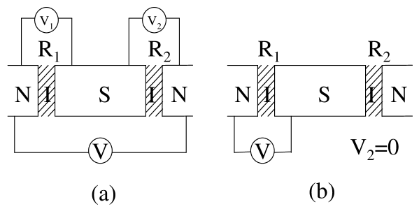
Figure 1: System of two NIS junctions with normal state resistances $R_{1}$ and $R_{2},$ $R_{1}>R_{2}.$ The junction number 1 cools the left normal electrode. The right normal electrode is a quasiparticle trap. Two possible bias methods are shown: (a) the bias voltage is applied between the normal metal leads, $V_{1}\not=0,$ $V_{2}\not=0$ and $V=V_{1}+V_{2};$ (b) the bias voltage is applied between the left normal lead and the superconductor, while the voltage drop at the second junction is zero, in this case $V=V_{1}$ and $V_{2}=0.$

The aim of this contribution is to consider processes in the superconducting electrode in more detail and obtain some quantitative estimations of the effectiveness of quasiaprticle traps.

The quasiparticles injected into superconductor by NIS junction create a nonequilibrium distribution which is characterized by the so called charge (or branch) imbalance. The number of electron-like excitations in not equal to the number of hole-like ones any more. This effect is known since 1972, when Clarke has carried out first experiments on charge imbalance [1] with NIS junctions. Under the existence of charge imbalance the simple formula (1) is not applicable and should be modified. Below we will modify it applying a method proposed by Tinkham [2, 3]. Then we consider a model NISIN system with two junctions in series (Fig.1). We assume that the resistance of the first junction ($R_{1}$) is high, while the resistance of the second one ($R_{2}$) is low. In this case the first junction cools the left normal electrode, while the second junction partially removes excited quasiparticles from the superconductor. The right normal metal lead models the quasiparticle trap [14]. For the sake of simplicity we assume that the junction number 2 is a tunnel junction and neglect proximity effect.

2 Theory

In this section we closely follow the method proposed by Tinkham [3].

Let us first consider a single NIS junction. For the sake of definiteness we choose the junction number 1. The Hamiltonian of the system can be written as follows:

$$\widehat{H}=\widehat{H}_{N}+\widehat{H}_{S}+\widehat{H}_{T},$$ (2)

where $\widehat{H}_{N}$ is the Hamiltonian of normal metal, $\widehat{H}_{S}$ is the Hamiltonian of superconductor and $\widehat{H}_{T}$ is the tunnel Hamiltonian. They are given by the following expressions:

$$\widehat{H}_{N} = \sum_{k,\alpha}(\epsilon_{k}-eV_{1})c^{+}_{k,\alpha}c_{k,\alpha},$$

$$\widehat{H}_{S} = \sum_{n,\alpha}\left\{\xi_{n}-E_{n}+E_{n}\gamma^{+}_{n,\alpha}\gamma_{n,\alpha}\right\},$$

$$\widehat{H}_{T} = \sum_{k,n,\alpha}\left\{t_{kn}c^{+}_{k,\alpha}a_{n,\alpha}+t^{*}_{kn}a^{+}_{n,\alpha}c_{k,\alpha}\right\}=\sum_{k,n,\alpha}\big{\{}t_{kn}c^{+}_{k,\alpha}[u_{n}\gamma_{n,\alpha}-\alpha v^{*}_{n}\bar{\gamma}^{+}_{n,-\alpha}]$$ (3)

$$+\;t^{*}_{kn}[u_{n}^{*}\gamma^{+}_{n,\alpha}-\alpha v_{n}\bar{\gamma}_{n,-\alpha}]c_{k,\alpha}\big{\}}.$$

Here $V_{1}$ is the potential of the first normal metal lead relative to the superconductor, $\epsilon_{k}$ is the energy of electrons in the normal metal referred to the appropriate chemical potential, $E_{n}=\sqrt{\xi^{2}_{n}+\Delta^{2}}$ is the energy of quasiparticles in the superconductor and $\xi_{n}$ are the energies of electrons in the superconductor ( $\xi_{n}$ has the same meaning as $\epsilon_{k}$ in the normal electrode). The index $k$ enumerates the states in the normal metal, $n$ does the same in the superconductor, while $\alpha=\pm 1$ is the spin index. We have also defined the creation $c^{+}_{k,\alpha}$ and annihilation $c_{k,\alpha}$ electron operators in the normal metal, analogous operators $a^{+}_{n,\alpha}$ and $a_{n,\alpha}$ in the superconductor, and quasiparticle operators $\gamma^{+}_{n,\alpha}$ and $\gamma_{n,\alpha}.$ The latter operators are related to the electron operators by means of the standard transformation $a_{n,\alpha}=u_{n}\gamma_{n,\alpha}-\alpha v_{n}^{*}\bar{\gamma}^{+}_{n,-\alpha},$ where the operator $\bar{\gamma}^{+}_{n,-\alpha}$ creates a quasiparticle in the state which is time reversed with respect to the $n$-th state and also carries an opposite spin. Finally, the BCS coherence factors are given by the following standard expressions: $|u_{n}|^{2},\,|v_{n}|^{2}=\frac{1}{2}\left(1\pm\frac{\xi_{n}}{E_{n}}\right).$

We consider the tunneling Hamiltonian as a perturbation. The current operator in interaction representation can be defined as the rate of tunneling out of the normal metal multiplied by the electron charge $-e$:

$$\widehat{I}=(-e)\bigg{(}-\frac{d}{dt}\sum_{k,\alpha}c^{+}_{k,\alpha}c_{k,\alpha}\bigg{)}=ie\bigg{[}\widehat{H}_{T},\sum_{k,\alpha}c^{+}_{k,\alpha}c_{k,\alpha}\bigg{]}.$$ (4)

The average value of the current can be evaluated by means of Fermi golden rule:

$$I = \langle\widehat{I}(t)\rangle=i\int\limits_{-\infty}^{t}dt^{\prime}\,\langle[\widehat{H}_{T}(t^{\prime}),\widehat{I}(t)]\rangle$$

$$= 4e\;{\rm Re}\sum_{k,n}|t_{kn}|^{2}\int\limits_{-\infty}^{t}dt^{\prime}\biggl{[}|u_{n}|^{2}{\rm e}^{i(E_{n}-\epsilon_{k}+eV_{1})(t-t^{\prime})}(f_{S,n}-f_{N,k})$$

$$+|v_{n}|^{2}{\rm e}^{-i(E_{n}+\epsilon_{k}-eV_{1})(t-t^{\prime})}(1-f_{N,k}-f_{S,n})\biggr{]}.$$

Evaluating time integrals we obtain

$$I = 4\pi e\,\sum_{k,n}|t_{kn}|^{2}\biggl{[}\delta(E_{n}-\epsilon_{k}+eV)|u_{n}|^{2}(f_{S,n}-f_{N,k})$$ (5)

$$+\delta(E_{n}+\epsilon_{k}-eV)|v_{n}^{2}|(1-f_{N,k}-f_{S,n})\biggr{]}.$$

Now, as usual, we replace $|t_{kn}|^{2}$ by constant value $|t|^{2},$ introduce densities of states in both leads, assume the distribution functions depend only on energy, and find

$$I_{1} = \frac{1}{eR}\int d\xi\left[\frac{1}{2}\left(1+\frac{\xi}{E}\right)(f_{S}(\xi)-f_{N}(E+eV_{1}))\right.$$ (6)

$$\left.+\frac{1}{2}\left(1-\frac{\xi}{E}\right)(1-f_{S}(\xi)-f_{N}(-E+eV_{1}))\right].$$

where $1/R=4\pi e^{2}|t|^{2}N_{0}^{N}N_{0}^{S}{\cal V}^{N}{\cal V}^{S},$ and ${\cal V}^{N,S}$ are the volumes of the normal and superconducting leads respectively. This result has been first derived by Tinkham [3]. Only if the distribution function in the superconductor satisfies the particle-hole symmetry requirement $f_{S}(-\xi)=f_{S}(\xi)$, and the distribution function in the normal metal satisfies $f_{N}(-E)=1-f_{N}(E)$ Eq. (6) reduces to the standard one:

$$I_{1}^{\rm sym}=\frac{1}{eR}\int dE\,\frac{\theta(E^{2}-\Delta^{2})|E|}{\sqrt{E^{2}-\Delta^{2}}}[f^{S}(E)-f^{N}(E+eV_{1})].$$ (7)

Note that there exist a difference in definition between the distribution functions $f_{S}(\xi)$ in (6) and $f_{S}(E)$ in (7). In the first case the distribution function depends on the energy of bare electrons in superconductor $\xi,$ while in the second case — on $E=\sqrt{\xi^{2}+\Delta^{2}}.$ Moreover, negative values of $E$ are allowed in (7), the distribution function for such values is defined by means of the relation $f_{S}(-E)=1-f_{S}(E).$

The cooling power of the normal metal is obtained analogously. First we note that $P_{1}=-\frac{d}{dt}\sum_{k,\alpha}\epsilon_{k}c^{+}_{k,\alpha}c_{k,\alpha},$ and then repeat all the steps of the previous procedure. Thus we find

$$P_{1} = \frac{1}{e^{2}R}\int d\xi\left[\frac{E+eV_{1}}{2}\left(1+\frac{\xi}{E}\right)(f_{N}(E+eV_{1})-f_{S}(\xi))\right.$$ (8)

$$\left.+\frac{E-eV_{1}}{2}\left(1-\frac{\xi}{E}\right)(1-f_{S}(\xi)-f_{N}(-E+eV_{1}))\right].$$

Again we note that only if $f_{S}(-\xi)=f_{S}(\xi)$ and $f_{N}(-E)=1-f_{N}(E)$ the latter result reduces to a simple formula (1).

The same approach can be applied in order to find the rates of population and depopulation of quasiparticle states in superconductor. Here we already consider the system of two junctions. We find

$$\frac{df_{S,n}}{dt} = \frac{d}{dt}\langle\gamma^{+}_{n,\alpha}\gamma_{n,\alpha}\rangle=-\frac{f_{S,n}-f_{0}(E_{n})}{\tau_{0}}$$ (9)

$$+\frac{|u_{n}|^{2}f_{N,1}(E_{n}+eV_{1})+|v_{n}|^{2}(1-f_{N,1}(-E_{n}+eV_{1}))-f_{S,n}}{2e^{2}R_{1}N_{0}^{S}{\cal V}^{S}}$$

$$+\frac{|u_{n}|^{2}f_{N,2}(E_{n}-eV_{2})+|v_{n}|^{2}(1-f_{N,2}(-E_{n}-eV_{2}))-f_{S,n}}{2e^{2}R_{2}N_{0}^{S}{\cal V}^{S}},$$

where $f_{N,1}$ and $f_{N,2}$ are the distribution functions is the two normal metal electrodes, $f_{0}(E)=1/(\exp(E/T)+1),$ and $\tau_{0}$ is the inelastic quasiparticle relaxation time in the superconductor. We use a very simple relaxation term in Eq. (9) because we actually do not consider the effect of quasiparticle interactions here. The relaxation term is introduced in the Eq. (9) only in order to establish the limitations of a non-interacting model. The second term in the right hand side of Eq. (9) describes the injection of quasiparticles through the first junction, while the last term – the injection through the second junction. The equations similar to Eq. (9) are derived and discussed in Ref. [6, 7, 9].

In a stationary case, $\dot{f}_{n}^{S}\equiv 0,$ the distribution function of quasiparticles in the superconductor can be found explicitly:

$$f_{S}(\xi) = \frac{1}{{\frac{N_{0}^{S}{\cal V}^{S}}{\tau_{0}}+\frac{1}{2e^{2}R_{1}}+\frac{1}{2e^{2}R_{2}}}}\left\{\frac{N_{0}^{S}{\cal V}^{S}}{\tau_{0}}f_{0}(E)\right.$$ (10)

$$\left.+\,\frac{1}{2e^{2}R_{1}}[|u|^{2}f_{N,1}(E+eV_{1})+|v|^{2}f_{N,1}(E-eV_{1})]\right.$$

$$\left.+\,\frac{1}{2e^{2}R_{2}}[|u|^{2}f_{N,2}(E-eV_{2})+|v|^{2}f_{N,2}(E+eV_{2})]\right\}.$$

Here we have assumed that the distribution functions in the normal metal electrodes satisfy $f^{N}_{1,2}(-E)=1-f^{N}_{12}(E).$ The result (10) is similar to that obtained in Ref. [9], but it includes the effects of charge imbalance which become important if the resistances $R_{1}$ and $R_{2}$ are not equal.

The shape of the quasiparticle distribution function (10) depends on two parameters: the junction asymmetry parameter $\alpha=R_{2}/(R_{1}+R_{2})$ and the ratio of inelastic relaxation rate to the injection rate $\beta={2e^{2}R_{1}N_{0}^{S}{\cal V}^{S}}/{\tau_{0}}.$ One can neglect inelastic relaxation as long as $\beta\ll 1.$ Here we have also assumed that quasiparticle distribution function does not depend on space coordinates. This assumption is valid if the appropriate size of the superconducting electrode does not exceed the quasiparticle relaxation length $L_{in}=\sqrt{D\tau_{0}},$ where $D$ is the diffusion constant.

Finally, the superconducting gap is determined by BCS gap equation:

$$1=\frac{\lambda}{2}\int d\xi\,\frac{1-2f_{S}(\xi)}{\sqrt{\xi^{2}+\Delta^{2}}},$$ (11)

where $\lambda$ is the electron-phonon coupling constant.

3 Results and discussion

Figure 2: Quasiparticle distribution function in the superconductor for different values of the parameters. (1) Dotted line – equilibrium distribution function $f_{0}(\xi)=1/[1+\exp(E/T_{eff})]$ with effective temperature $T_{eff}/\Delta_{0}=0.3.$ (2) Solid line – bias voltage is applied between normal metals (Fig. 1a), $eV/\Delta_{0}=1.72,$ $T/\Delta_{0}=0.1,$ $\alpha=0.05,$ no inelastic relaxation ($\beta=0$). (3) Dashed line – all parameters have the same values as in the previous case, but the inelastic relaxation time is finite, $\beta=10.$ (4) Short dot – bias voltage is applied between normal metal and superconductor (Fig. 1b), $eV/\Delta_{0}=1,$ $T/\Delta_{0}=0.1,$ $\alpha=0.05,$ $\beta=0.$

We have solved the set of equations (6,8,10) numerically. It has been done as follows. First, we have chosen the equilibrium distribution functions with the same temperature $T$ in both normal metal leads. If the bias voltage is applied between the normal metals, (Fig. 1a), then the voltages across individual junctions are fixed by the current conservation requirement $I_{1}(V_{1})=I_{2}(V_{2})$ and $V_{1}+V_{2}=V.$ These equations are solved numerically. If only the junction number 1 is biased (Fig. 1b), then we just set $V_{1}=V,$ $V_{2}=0.$ As long as $V_{1}$ and $V_{2}$ are known, we find the distribution function (10) and the cooling power (8). Below we present some results. All energy scales are normalized by the superconducting gap at zero temperature, $\Delta_{0}\equiv\Delta(T=0).$

Fig. 2 shows the distribution function for different sets of the parameters. In all cases this function has an asymmetry with respect to the chemical potential of Cooper pairs, this a manifestation of charge imbalance. This effect turns out to be relatively weak if the bias voltage is applied between the normal metals. Once again we note that the distribution function does not look like a Fermi function because of its definition (see the discussion after Eq. (7)).

Figure 3: Cooling power for different junctions asymmetry and in the absence of the inelastic relaxation. (a) The voltage is applied between two normal metals (Fig. 1a). (b) The voltage is applied between the normal metal and the superconductor (Fig. 1b).

The cooling power of the first junction (8) as function of voltage is shown in Fig. 3. We have neglected inelastic processes in superconductor assuming $\beta\ll 1.$ We observe that even a relatively small resistance of the second junction may significantly reduce the cooling power. It is quite natural because the cooling of the superconductor becomes less effective. In the opposite case $\beta\gg 1$ the cooling power is given by the standard formula (1). However, in this case the power dissipated in the superconductor goes first to the phonon subsystem, and then may return back to the cooled normal metal [12]. This effect may strongly reduce the overall cooling power of the device. In the absence of inelastic relaxation such processes are less probable, because power dissipation takes place in the normal metal with high heat conductivity and the heat is effectively removed from the device. That’s why below we consider the case $\beta\ll 1.$

Figure 4: Dependence of maximum cooling power on temperature. Inelastic relaxation in superconductor is neglected. Solid line – maximum cooling power at $\alpha=0.05$ and bias voltage applied between the normal metal leads (Fig. 1a). Dotted line – maximum cooling power at $\alpha=0.05$ and bias voltage applied to the first junction (Fig 1b). Dashed line – equilibrium result based on Eq. (1), $P_{1}^{\max}=0.6({\Delta_{0}^{2}}/{e^{2}R_{1}})({T}/{\Delta_{0}})^{3/2}$ [11].

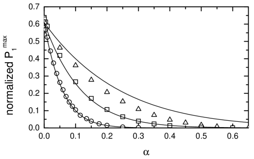
Figure 5: Dependence of maximum cooling power on asymmetry $\alpha.$ $\beta=0,$ voltage is applied to the first junction (Fig. 1b). The cooling power is normalized by $({\Delta_{0}^{2}}/{e^{2}R_{1}})({T}/{\Delta_{0}})^{3/2}.$ Triangles, squares and circles — numerical results for $T/\Delta_{0}=0.2,\;0.1,\;0.05$ respectively. Solid lines — simple approximation (12).

The dependence of the maximum cooling power on temperature is illustrated in Fig. 4. The cooling power is drastically reduced at low temperatures $T/\Delta_{0}<\alpha.$ Fig. 5 shows the dependence of the maximum cooling power on the asymmetry $\alpha.$ Here we again observe the reduction of the cooling power for $\alpha>T/\Delta_{0},$ in agreement with the Fig. 4. If the bias voltage is applied only to the first junction and the temperature is much lower than $\Delta_{0}$, one can get an approximate analytical expression for the maximum cooling power:

$$P_{\rm 1,max}=\frac{\Delta_{0}^{1/2}T^{3/2}}{e^{2}R_{1}}\left[0.76{\rm e}^{-\left(\frac{\Delta_{0}}{T}-\frac{1}{8}\right)\alpha}-0.22{\rm e}^{-2\left(\frac{\Delta_{0}}{T}-\frac{1}{8}\right)\alpha}+0.07{\rm e}^{-3\left(\frac{\Delta_{0}}{T}-\frac{1}{8}\right)\alpha}\right].$$ (12)

If the voltage is applied to the normal metal electrodes, the maximum cooling power is even lower than (12).

Figure 6: The suppression of superconducting gap at different degrees of asymmetry. The bias voltage is applied to the normal metal electrodes (Fig. 1a).

Fig. 6 shows the suppression of the gap due to the heating of the superconductor.

The model employed above requires two conditions to be satisfied: the size of the superconductor should be less than $L_{in},$ and $\beta$ should be small, $\beta\ll 1.$ Experimentally one finds $L_{in}$ to be of the order of at least several microns (see e.g. [14, 13]). Thus, the first requirement is not very restrictive, although it may depend on sample geometry. The parameter $\beta$ is difficult to estimate because the inelastic relaxation time is unknown. Most probably this time is of the order of several microseconds (see e.g. [4]). If so, then the condition $\beta\ll 1$ can also be easily satisfied in experiment.

In conclusion, we have derived a generalized expression for the cooling power of a NIS tunnel junction taking into account charge imbalance effects. We have considered cooling properties of NISIN double junction structure. The interactions in the superconductor were neglected. Such an approximation is applicable provided the superconducting electrode is of submicron size. It is shown that the cooling power depends strongly on the ratio of the resistances of the two junctions. We have shown that at low temperatures the maximum cooling power of NISIN structure is proportional to $\exp(-\Delta_{0}R_{2}/T(R_{1}+R_{2})).$

References

- [1] J. Clarke, Experimental observation of pair-quasiparticle potential difference in nonequilibrium superconductors, Phys. Rev. Lett. 28(21), 1363-1366 (1972).
- [2] M. Tinkham and J. Clarke, Theory of pair-quasiparticle potential difference in nonequilibrium superconductors, Phys. Rev. Lett. 28(21), 1366-1369 (1972).
- [3] M. Tinkham, Tunneling generation, relaxation, and tunneling detection of hole-electron imbalance in superconductors, Phys. Rev. B 6(5), 1747-1756 (1972).
- [4] S.B. Kaplan, C.C. Chi, D.N. Langenberg, J.J. Chang, S. Jafarey, and D.J. Scalapino, Quasiparticles and phonon lifetimes in superconductors, Phys. Rev. B 14(11), 4854-4873 (1976).
- [5] G.J. Dolan and L.D. Jackel, Voltage measurements within the nonequilibrium region near phase-slip center, Phys. Rev. Lett. 39(25), 1628-1631 (1977).
- [6] C.J. Pethick and H. Smith, Relaxation and collective motion in superconductors: a two-fluid description, Ann. of Phys. 119, 133-169 (1979).
- [7] J. Clarke, Experiments on charge imbalance in superconductors, in: Nonequilibrium superconductivity, edited by D.N. Langenberg and A.I. Larkin, (Elsevier Science Publishers B.V., 1986), pp. 1-63.
- [8] M. Johnson and R.H. Silsbee, Nonequilibrium superconductivity: new crystallographic and magnetic field efects, Phys. Rev. Lett. 58 (26), 2806-2809 (1987).
- [9] D.R. Heslinga and T.M. Klapwijk, Enhancement of superconductivity far above the critical temperature in double-barrier tunnel junctions, Phys. Rev. B 47 (9), 5157-5164 (1993).
- [10] M. Nahum, T.M. Eiles, and J.M. Martinis, Electronic microrefrigerator based on a normal metal-insulator-superconductor tunnel junction, Appl. Phys. Lett. 65, 3123-3125 (1994).
- [11] M.M. Leivo, J.P. Pekola, D.V. Averin, Efficient Peltier refrigeration by a pair of normal metal/insulator/superconductor junctions, Appl. Phys. Lett. 68 (14), 1996-1998 (1996).
- [12] J. Jochum, C. Mears, S. Golwala, B. Sadoulet, J.P. Castle, M.F. Cunningam, O.B. Drury, M. Frank, S.E. Labov, F.P. Lipschultz, H. Netel, and B. Neuhauser, Modeling the power flow in normal conductor-insulator-superconductor junctions, J. Appl. Phys. 83 (6), 3217-3224 (1998).
- [13] J.N. Ullom, P.A. Fisher, and M. Nahum. Energy-dependent quasiparticle group velocity in a superconductor, Phys. Rev. B 58(13), 8225-8228 (1998).
- [14] J.P. Pekola, D.V. Anghel, T.I. Suppula, J.K. Suoknuuti, A.J. Manninen, and M. Manninen, Trapping of quasiparticles of a nonequilibrium superconductor, Appl. Phys. Lett. 76(19), 2782-2784 (2000).