Analytical modeling for the heat transfer in sheared flows of nanofluids

Abstract

We developed a model for the enhancement of the heat flux by spherical and elongated nano-particles in sheared laminar flows of nano-fluids. Besides the heat flux carried by the nanoparticles the model accounts for the contribution of their rotation to the heat flux inside and outside the particles. The rotation of the nanoparticles has a twofold effect, it induces a fluid advection around the particle and it strongly influences the statistical distribution of particle orientations. These dynamical effects, which were not included in existing thermal models, are responsible for changing the thermal properties of flowing fluids as compared to quiescent fluids. The proposed model is strongly supported by extensive numerical simulations, demonstrating a potential increase of the heat flux far beyond the Maxwell-Garnet limit for the spherical nanoparticles. The road ahead which should lead towards robust predictive models of heat flux enhancement is discussed.

I Introduction

The enhancement of heat transfer by embedded nano-particles in a fluid subjected to a temperature gradient is an important issue that is expected to help in technological application like solar heating, and various cooling devices, including miniaturized computer processors. Accordingly, many experiments were conducted in the last couple of decades Rev2011a ; Rev2011b ; Rev2010a ; Rev2009a ; Rev2009b , with a breakthrough announcement from a group at Argonne National Laboratory, who studied water and oil-based nanofluids containing copper oxide nanopaticles, and found an amazing 60% enhancement in thermal conductivity for only a 5% volume fraction of nanoparticles 96ECLTL . Subsequent research has however generated what Ref. 06KK referred to as “an astonishing spectrum of results”. Results in the literature show sometime enhancement in the thermal conductivity compared to the prediction of the Maxwell-Garnett effective medium theory, and sometime values that are less than the same prediction Rev2011a ; Rev2011b ; Rev2010a ; Rev2009a ; Rev2009b . Confusingly enough, these discrepancies occur even for the same fluid and the same size and composition of the nano-particles.

Some of these conflicting results were explained by either the formation of percolated clusters of particles (for the case of enhancement with respect to the Maxwell-Garret prediction) or by surface (Kapitza) resistance (for the case of reduction with respect to the same prediction) Rev2010a . Interestingly enough, enhancement is typically seen in quiescent fluids, and one expects that the agglomeration of clusters will become impossible in flows, be them laminar or turbulent. Of course, in technological application flowing nano-fluids may be the rule rather than the exception. Thus our aim in this article is to develop models of heat flux in flowing nano-fluids, where the flow can be either laminar or turbulent. In such systems we cannot expect an enhancement of heat flux due to the agglomeration of particles (at least at low volume fractions), and for the sake of simplicity we will assume that there is no Kapitza resistance. Since it was reported in the literature that elongated nano-particles are superior to spheres in quiescent nanofluids 97Nan , we will study both spheres and spheroids  in flowing nanofluids. We will argue that generically elongation may not be advantageous at all, and will explain why.

For completeness, we will begin by studying quiescent nanofluids under a temperature gradient. We will present extensive numerical simulation that will demonstrate a very good agreement with the Maxwell-Garnett theory for spherical nano-particles and with the generalization of Nan et al 97Nan for elongated particles. In the case of flowing nanofluid we will offer a model that will provide expressions for the heat transfer for different values of the aspect ratio of the particles, for different volume fractions and for laminar and turbulent flows.

The structure of the paper is as follows. In the next Section (II) we formulate the problem, describe the equations of motion and the numerical procedure, and discuss the dilute suspension approximation. In Section III we describe the results of numerical simulations of spherical and spheroidal particles in a fluid at rest and in a shear flow. In Section IV we develop an analytical model of heat transfer characteristic, i.e. the Nusselt number, and analyze the model predictions of heat flux enhancement in two limiting cases of very strong Brownian diffusion and a weak one.

II Nanofluids in the dilute limit

In this section we formulate the model for dilute nanofluids laden with elongated spheroidal nanoparticles. This includes the basic equation of motion for the velocity and temperature fields and the boundary conditions (with constant velocity and temperature gradients far away from particles). We also present details of the numerical simulations and their validation.

II.1 Formulation of the problem and the flow geometry

When the nanofluid is very dilute one can disregard the effect of one particle on the other and consider the nanofluid as an ensemble of noninteracting particles. One of these is shown in Fig. 1. The center of the spheroidal particle is at the position $x=y=z=0$ in the middle of a plane Couette flow between two $H$-separated horizontal parallel walls that move in the $\hat{x}$-direction with opposite velocities $V_{\pm}=\pm V/2$. Due to the symmetry, the forces are balanced, and the particle neither migrates nor collides with the walls; the particle’s center remains at $(0,0,0)$. This allows us to eliminate in the numerics any effect of the particle sweeping parallel to the walls. Note that this effect is anyway absent in homogeneous cases.

We employ periodic boundary conditions along the $x$ and the $z$ direction. This results in a periodic replication of the computational box (together with the particle) in the $XZ$-plane, leading to a “monolayer” of an infinite number of periodically distributed particles in the $XZ$-plane. Remarkably enough (and by reasons that will be explained below), this allows us to reproduce in numerics with a single particle effects of a finite volume fraction $\varphi$ at least up to $\varphi\lesssim 20\div 30\%$.

The walls are kept at fixed temperatures $T_{\pm}=T\pm\Delta/2$. In the absence of particles these boundary conditions give rise to a vertical temperature gradient $\nabla_{y}T=\Delta/H$ and shear $S=S_{xy}=V/H$ (see Fig. 1).

The spheroidal particle’s semi-axes are $a$ (the longest) and $b$ (the shortest), $a\geq b$ (Fig. 1). The thermal diffusivity inside the particle is $\chi_{\rm p}$. The carrier fluid has a kinematic viscosity $\nu$ and a thermal diffusivity $\chi_{\rm f}$. For simplicity, at this stage we neglect the effect of gravity and the particle mass. The co-ordinate system and polar angles are given by:

$$n_{x}=\, \cos\widetilde{\theta} \,=\sin{\theta}\sin{\phi}\,,$$ (1a)

$$n_{y}=\, \sin\widetilde{\theta}\sin\widetilde{\phi} \,=\sin{\theta}\cos{\phi}=\cos\theta_{\textrm{N}}\,,$$ (1b)

$$n_{z}=\, \sin\widetilde{\theta}\cos\widetilde{\phi} \,=\cos{\theta}\,,$$ (1c)

where $n_{i}$ is the projection of the unit-vector $\widehat{\bm{n}}$ onto the axis $i$, $i=\{x,y,z\}$, and $\theta_{\textrm{N}}$ is the angle between the particle’s largest axis and the $y$-axis.

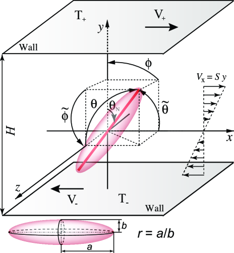
Figure 1: The particle in a plane Couette flow. The largest particle axis is shown as a (red) rod. The velocity field (far from the particle) is $(Sy,0,0)$ where the shear $S=(V_{+}-V_{-})/H$ in the particle-free flow with $H$ being the distance between the walls. For the theoretical development we assume the creeping flow conditions as in Jef ; Leal1971 ; Hinch1972 .

In the absence of particles, changing the intensity of the laminar shear flow does not change the heat flux since there is no velocity orthogonal to the wall and the system is homogeneous in the direction parallel to the wall. In the presence of a particle, the shear induces it to rotate, the simplest case being a spherical particle which rotates at a constant angular velocity $\Omega_{z}=S/2$ (provided the particle radius is much smaller than the distance to the wall). This rotation induces a vertical flow motion near the particle. The modification of the velocity profile has three consequences. The first directly affects the heat convection in the fluid through a convective contribution $v_{y}T$. The second comes from the particle rotation which brings up the hotter side of the particle during its rotation. The third changes the heat conduction due to a modification of the temperature profiles at the surface of the particle.

In the case of non spherical particles the presence of a shear has also a strong influence of the statistical distribution of particle orientations.

II.2 Dimensionless parameters

To fix the notation we list here the most important dimensionless parameters involved in the problem:

$$\mbox{aspect ratio:}\quad\quad\ r \equiv a/b\,,\quad\ r\geq 1\,,$$ (2a)

$$\mbox{diffusivities ratio:}\quad\quad\ k \equiv \chi_{\rm p}/\chi_{\rm f}\,,$$ (2b)

$$\mbox{Prandtl number:}\quad\ \ \mathrm{Pr} \equiv \nu/\chi_{\rm f}\,,$$ (2c)

$$\mbox{Reynolds number:}\quad\mathrm{Re} \equiv (2a)^{2}S/\nu\,,$$ (2d)

$$\mbox{Peclet number:}\quad\mathrm{Pe} \equiv (2a)^{2}S/\chi_{\rm p}\ .$$ (2e)

Note that the particle’s largest axis defines our length-scale. Also,

$$\mathrm{Pe}=\mathrm{Re}\,\mathrm{Pr}/k\ .$$ (3)

II.3 Basic equations of motion

The dynamical effects previously mentioned can be quantitatively studied by solving the following system of equations for the temperature in the fluid, $T_{\rm f}$, and in the particle, $T_{\rm p}$,

$$\frac{\partial T_{\rm f}}{\partial t}+(\bm{u}\cdot\bm{\nabla})T_{\rm f} = \chi_{\rm f}\nabla^{2}T_{\rm f}\,,\quad\frac{\partial T_{\rm p}}{\partial t}=\chi_{\rm p}\nabla^{2}T_{\rm p}\ .~{}~{}~{}~{}$$ (4a)

together with the boundary conditions,

at the surface: $$T_{\rm f}={T}_{\rm p}\,, \chi_{\rm f}{\nabla}T_{\rm f}=\chi_{\rm p}{\nabla}{T}_{\rm f}\,,$$

on the walls: $$T_{\rm f}(x,0,z)=T_{-}\,, T_{\rm f}(x,H,z)=T_{+}\ .$$

The fluid velocity in the whole domain can be found by solving the incompressible Navier-Stokes equations:

$$\frac{\partial\bm{u}_{\rm f}}{\partial t}+(\bm{u}_{\rm f}\cdot\bm{\nabla})\bm{u}_{\rm f}=-\frac{1}{\rho_{\rm f}}\bm{\nabla}p+\nu\nabla^{2}\bm{u}_{\rm f}\,,\quad\bm{\nabla}\cdot\bm{u}_{\rm f}=0\,,$$ (4b)

together with non-slip boundary conditions at the surface of the particle and at the walls:

$$\bm{u}_{\rm f}(x,0,z)=\{V_{-},0,0\}\,,\quad\bm{u}_{\rm f}(x,H,z)=\{V_{+},0,0\}\,,$$

$$\bm{u}_{\rm f}(x,y,z)=\bm{u}_{\rm p}(x,y,z)\ \ \mbox{at the particle's surface}.$$

Here $\rho_{\rm f}$ is the carrier fluid density and $p$ is the pressure. Clearly, on nano-scales the temperature difference (across a particle) is sufficiently small to allow us to neglect the dependence of the fluid’s and particle’s material parameters on the temperature, i.e. we take $\nu$, $\chi_{\rm f}$ and $\chi_{\rm p}$ as constants.

The dynamics of a neutrally buoyant particle is governed by the equations of the solid body rotation Allen :

$$\frac{d\,{\Omega}_{x}^{(\mathrm{b})}}{dt} = \frac{T_{x}^{(\mathrm{b})}}{I_{x}}+\frac{I_{y}-I_{z}}{I_{x}}\Omega_{y}^{(\mathrm{b})}\Omega_{z}^{(\mathrm{b})}\,,$$

$$\frac{d\,{\Omega}_{y}^{(\mathrm{b})}}{dt} = \frac{T_{y}^{(\mathrm{b})}}{I_{y}}+\frac{I_{z}-I_{x}}{I_{y}}\Omega_{z}^{(\mathrm{b})}\Omega_{x}^{(\mathrm{b})}\,,$$ (4c)

$$\frac{d\,{\Omega}_{z}^{(\mathrm{b})}}{dt} = \frac{T_{z}^{(\mathrm{b})}}{I_{z}}+\frac{I_{x}-I_{y}}{I_{z}}\Omega_{x}^{(\mathrm{b})}\Omega_{y}^{(\mathrm{b})}\,,$$

where $\bm{\Omega}^{(\mathrm{b})}$ is the angular velocity in the body-fixed frame, $\bm{T}^{(\mathrm{b})}$ is the torque in the body-fixed frame and $I$ is the moment of inertia tensor.

II.4 Numerical approach and its validation

The numerical simulation of the conjugated heat transfer problem given by Eqs (4) is performed by means of two coupled D3Q19 Lattice Boltzmann (LB) equations under the so-called BGK approximation Succi2001 . Details of the simulations are presented in Appendix A . Besides purely numerical means, the control of the simulations was done by its comparison with known analytical solutions. As an example, Fig 2 shows the comparison between the analytical temperature profile (28) (solid red line) and numerical profile (black dots) for a moderately big spherical particle [$H/(2R)=3.2$].

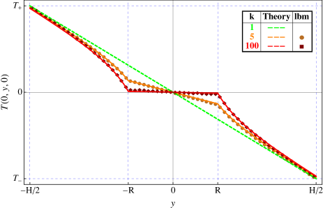
Figure 2: Temperature profile along a line passing through the center of a spherical particle (of radius $R$) in a quiescent fluid. Dashed (green) line – conductive temperature profile in the pure fluid, solid (red) curve – Eq. (28) LnL for an infinite domain with a temperature gradient, dots – numerical results (at lattice points) with $k=5$ (full circles) and $k=100$ (squares). The present test was performed with Pr $=1$, $H=64$ and $R=10$ lattice units.

The second test was the comparison in Fig. 10 of the particle’s angular velocity theoretically obtained by Jeffery Jef and simulated by our LB-realization. For more details, again see Appendix A.

II.5 From single particle modeling to finite volume fraction

Here we discuss how to relate the contribution of a single particle to the heat flux with the total contribution of many weakly-interacting particles randomly distributed in the flow occupying a finite volume fraction $\varphi$.

The first step is to consider fully dilute limit, $\varphi\to 0$, in which we can exploit the fact that the particle contribution is additive and proportional to $\varphi$. In this way we can introduce the Nusselt number as the ratio between the total heat flux (inside the computational cell) and the conductive heat flux in the basic cell:

$$\mbox{Nu}=\frac{\langle q\rangle}{\langle q_{\rm cond}\rangle}=\frac{-\chi_{\rm eff}\nabla_{y}T}{-\chi_{f}\nabla_{y}T}=\frac{\chi_{\rm eff}}{\chi_{f}}\,,$$ (5)

where $q$ is the total heat flux, $q_{\rm{cond}}=-\chi_{f}\nabla_{y}T$ is the conductive part and $\chi_{\rm eff}$ is the effective heat diffusivity of the composite fluid. Also, $\nabla_{y}T\equiv{\partial T(x,y,z)}/{\partial y}$. Without particles $\langle q\rangle=\langle q_{\rm{cond}}\rangle$ and Nu $=1$. For dilute suspensions, in which $\varphi\ll 1$, Nu can be expanded in powers of $\varphi$ Jeff73 :

Nu $$= 1+\varphi\,K(\varphi)\,,$$ (6a)

$$K(\varphi) = K_{1}+K_{2}\,\varphi+\dots\,,$$ (6b)

where $K_{i}$ are dimensionless constants dependent on the Peclet number, on the particle’s aspect ratio, $r$, on the relative heat diffusivity, $k$, and maybe other parameters like Reynolds or Prandtl numbers [see Eqs. (2)], i.e. $K_{j}=K_{j}(\mbox{Pe},r,k,\dots)$.

As expected, in our simulations the quantity $($Nu$-1)$ is indeed proportional to $\varphi$ for $\varphi\lesssim 0.05$. This allows us to find $K_{1}$ as a function of other parameters (2) of the problem.

The next order term in the expansion (6b), i.e. $K_{2}\,\phi$, contains very important information about how Nu depends on $\varphi$ for small but finite values of $\varphi$. Generally speaking, to get this information from numerics one needs to solve Eqs. (4) for many particles, randomly distributed in space. We demonstrate that this problem can be tremendously simplified by reducing it to a one-particle case, in which this particle of volume $V{{}_{\rm{p}}}=\varphi V{{}_{\rm{cell}}}$ is put in the center of computational box of volume $V_{\rm{cell}}$ with periodic boundary conditions in the horizontal (orthogonal to the temperature gradient) $x$- and $z$-directions. In this way the total system can be considered as constructed from a periodic repetition of the basic elementary cell in the $x$- and $z$-directions. Comparing in Subsec. III.1.1 our numerical results with analytical findings obtained under the assumption of random particle distributions, we see that the precise particle distribution is not essential – what really matters is the actual volume fraction.

The reason for that is quite simple: as one sees in Fig. 2, the deviation from the linear temperature profile becomes important at distances  smaller than the particle diameter $2R$ for both $k=5$ and $k=100$. Thus any nonlinear dependence of Nu on $\varphi$ can appear only if the particles are sufficiently close to overlap the deviation from linear temperature profile. We see from our numerics that the this interaction causes 10% deviation from the straight line in Nu vs. $\varphi$ dependence for volume fractions of about 0.1 and more for $k\leq 100$. For $\varphi>0.1$ there is some nonlinear dependence of Nu on $\varphi$ but it practically coincides for the random and the periodic distributions of particles.

III Towards an analytical model of the heat flux

In this Section we begin with collecting the required information about the dependence of $K_{j}$ on the various parameters (2). To do this we consider simple limiting cases, for which some of these parameters are put to zero. We start with the case of spherical particles.

III.1 Spherical nano-particles

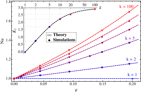
Figure 3: (Color online). Quiescent fluid, spherical particle in the center. Nu$(\varphi)$. Dashed curves – theory, Eq. (7) and dots – simulations for different $k$ (color-coded from “cold”-blue, $k=1$, to “hot”-red, $k=100$). Insert: $K_{1}(k)$. Dashed curve – theory, Eq. (7) and dots – simulations for different $k$ (same color-code). Notice, that for $128^{3}$ runs the accuracy is better then $0.3$%, while for $64^{3}$ runs it is about $0.7$%, and only for really small $32^{3}$ runs it reaches the worst value of $1.5$%. These means that for our purposes, usually the runs with $64^{3}$ box is fully satisfactory.

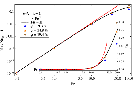
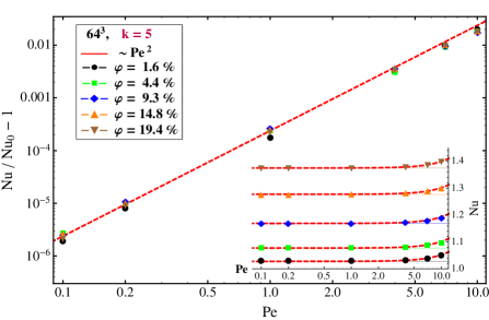
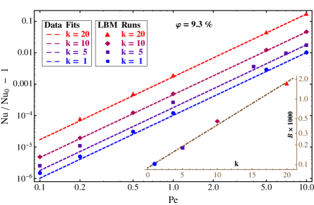
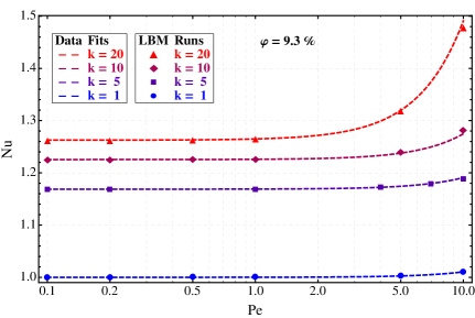
Figure 4: (Color online). A spherical particle in a shear (Couette) flow. Upper left panel: $k=1$, $\varphi=9.3\%,14.8\%$ and 19.4%. Upper right panel: $k=5$ for wider region of $\varphi$, but Pe is limited by 10. Both upper panels show Nu(Pe)/Nu${}_{0}-1$ vs. Pe, and both insets show Nu(Pe) vs. Pe. Here Nu${}_{0}\equiv\,$Nu$(0)$. Dashed (red) line is a fit $\propto$ Pe², cf. Eq. (8a); (color) symbols are simulations with different volume fractions: $\varphi=$ 1.6%, 4.4%, 9.3%, 14.8%, 19.4%. Solid (black) curve on upper left panel represents the fit by Eq. (9). Lower panels: $\varphi=9.3\%$ and different $k$ (from “cold”-blue, $k=1$, to “hot”-red, $k=20$). Dashed (”temperature”-colored) lines are fits to simulated data (symbols, same colors) by Eq. (8a), left panel, and by combined Eqs. (III.1.2) and (7), right panel. Inset on lower left panel: $B(k,\varphi)$ vs $k$ at $\varphi=9.3\%$. Dot-dashed (brown) line is the fit to Eq. (8b). Parameters: $64^{3}$, Pr $=1$, thus, $\mathrm{Re}=\mathrm{Pe}\,k$.

III.1.1 Test case: s spherical nano-particle in a fluid at rest

Here we consider the simplest case of a spherical particle ($r=1$) in a fluid at rest (Re = Pe = 0). Chiew and Glandt chiew suggested the following formula for this case:

$$K(k,\varphi) \simeq \frac{3\,K_{1}(k)}{3-K_{1}(k)\varphi}\,,\quad K_{1}(k)=3\,\frac{k-1}{k+2}\,,~{}~{}~{}~{}$$ (7a)

Nu $$= 1+\frac{3\,K_{1}(k)\,\varphi}{3-K_{1}(k)\,\varphi}\ .$$ (7b)

We notice that the expression for $K_{1}(k)$ which controls the very dilute limit ($\varphi\to 0$) is the same as in the Maxwell model Max . Obviously, for $k=1$ one has zero effect, i.e. Nu $=1$. For $k\to\infty$, $K_{1}=3$ and one has maximal possible enhancement (at fixed $\varphi\ll 1$). For $k=2$ one has 25% of this value, $k=4$ gives already 50% of the effect, $k=10\Rightarrow 75\%$, $k=20\Rightarrow 86\%$ and $k=100\Rightarrow 97\%$. Clearly, the larger $k$ the better, but increasing $k$ above 100 is not effective.

Actually, Eq. (7) includes also information about the nonlinear dependence $K(\varphi)$. However this dependence is very weak in the relevant range of parameters: e.g. for $k=10$ and $\varphi=0.2$ the difference between $K(\varphi)$ and its linear approximation is only 15%. For smaller $k$ this difference is even smaller. The physical reason for that was explained at the end of previous Section.

We tested the prediction of Eq. (7) by simulating the heat flux in a periodic box as explained above in Sec. II and in Appendix A. For the fluid at rest the (volume averaged) Nusselt number (as a function of $\varphi$ at different values of $k$) was measured and is shown in Fig. 3, where the inset shows $K_{1}(k)$. The overall conclusion is that

Eq. (7) agrees extremely well with all our simulations and thus can be used in modeling the effect of spherical particles in a fluid at rest.

III.1.2 Spherical nano-particle in a shear flow

The next important question is how the particle rotation affects the heat flux. As already mentioned, this rotation induces fluid motions around the particles thus causing convective contribution to the heat flux. This changes the temperature profile around the particles and, in turn, affects the heat flux inside the particles. To study these issues analytically is extremely difficult and thus numerical simulations can play a crucial role. Due to the fact that we have to deal with a number of parameters, we will carefully examine them starting with the simplest case of spherical particles. Results for spheroidal particles are discussed in Sec. III.2.2.

We begin by considering the case $k=1$; such a particle at rest does not affect the heat flux, thus Nu $=1$. In Fig. 4, upper left panel, we present Nu(Pe)/Nu$(0)-1$ as a function of Pe for $k=1$ at various volume fractions (from 9.3% to 19.4%), while the inset is showing Nu vs. Pe. Observing the data, we suggest for Pe$\lesssim 10$ the following ansatz

$$\mbox{Nu(Pe)}\simeq\mbox{Nu}(0)[1+B(k,\varphi)\mbox{Pe}^{2}]\,,$$ (8a)

shown in this panel as a straight dashed (red) line. One sees that Eq. (8a) is approximately valid up to Pe $$\simeq 10 k=1 B B(1,\varphi)\simeq 10^{-4} k=5 B(5,\varphi)\simeq 2.5\cdot 10^{-4}$$, where the deviation is about 1%. We note also that for the value of is very small, . A similar analysis for , (cf. Fig. 4, upper right panel), shows that Eq. (8a) fits the data even better with a similar value .

We see that $B$ depends weakly on $\varphi$ but more strongly on $k$. Thus, to determine the leading $k$-dependence we put a sphere of radius 18 in a $64^{3}$ computational volume (all in lattice units); this is equivalent to $\varphi\simeq 9.3\%$, see Fig. 4, lower panels. The $k$-dependence of $B(k,\varphi)$ in Eq. (8a) in the range of $\varphi\simeq 10\%$ can be fitted by:

$$B(k,\varphi) \simeq B_{1}(\varphi)\,\exp\left[B_{2}(\varphi)\,k\right],$$ (8b)

$$B_{1} \simeq 9\!\times\!10^{-5},\ B_{2}\simeq 0.15\ .$$ (8c)

For larger Pe$\gtrsim 10$ , the Nu vs. Pe dependence deviates down, as expected, because at Pe $\to\infty$ this dependence should saturate. Our analysis shows that this dependence can be fitted with a good accuracy by the formula that generalizes Eq. (8a):

$$\frac{\mbox{Nu(Pe)}}{\mbox{Nu}(0)}-1\simeq\frac{B(k,\varphi)\ \mbox{Pe}^{2}}{1+\mbox{Pe}/\mbox{Pe}_{1}(k)+[\mbox{Pe}/\mbox{Pe}_{2}(k)]^{2}}\ .$$ (9)

The upper left panel in Fig. 4 shows by a solid (black) curve how this model works for $k=1$ (with Pe${}_{1}(1)\approx 61$ and Pe${}_{2}(1)\approx 63$).

Having in mind that in many applications related to nanofluids the value of Pe is smaller than 0.01 and in any case rarely exceeds unity, we reach the conclusion that the convective heat flux around spherical particles and variations of the heat flux inside spherical particles due to their rotation can be neglected. Equation (7) can be used to model the heat flux enhanced by spherical nano-particles with finite volume fraction up to 25% and any actual value of $k$ in fluids at rest and in shear flows.

The next question to consider is the effect of the particle shape. We will begin with the case of spheroidal particles in fluids at rest.

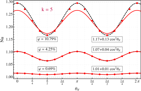
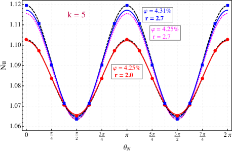
Figure 5: (Color online) Spheroid in a quiescent fluid at different angles $\theta_{\rm N}$. Both panels: $k=5$, Pr = 1, $64^{3}$. Symbols – simulations, solid (red or blue) curves – Eq. (11) with appropriate $r$ and $\varphi$, dashed (black) curves – fits by Eq. (10) to the simulations. Upper panel: $r=2$. Data: $\varphi\simeq 10.79\%$ (upper), $\varphi\simeq 4.25\%$ (middle) and $\varphi\simeq 0.69\%$ (lower). The largest mismatch between the simulations and Eq. (11) is 2.8% at $\varphi=10.79\%$. Lower panel: lower (red) dots: $\varphi=4.25\%$, $r=2.0$, and upper (blue) squares: $\varphi=4.31\%$, $r=2.7$. The dotted (magenta) curve is Eq. (11) with $\varphi=4.25\%$ and $r=2.7$. The effect of changing $r$ is larger than that of $\varphi$.

III.2 Spheroidal nano-particles

III.2.1 Spheroidal nano-particle in a fluid at rest

The general expectation is that spheroidal nano-particles should be able to enhance the heat flux much more effectively then spherical particles. To achieve this they have to be oriented in the “right” direction, i.e. along with the temperature gradient. Therefore, logically, the study of the heat flux in nanofluids laden with spheroids should begin with the clarification of the effect of the spheroid orientation on the heat flux. In this Section we consider this effect for a given and fixed orientation of the spheroids. For this purpose we perform numerical simulations of the heat flux with spheroidal nano-particles in a quiescent fluid (Pe$=0$) with a temperature gradient, see Fig. 1, taking for concreteness $k=5$.

For different orientations of the spheroid (i.e. different $\theta_{\rm N}$ – the angle between the temperature gradient vector and the largest spheroid’s axis), we measure different Nusselt numbers: when $\theta_{\rm N}=0$ spheroids with higher conductivities tend to forms a thermal shortcut, thus Nu is larger than for $\theta_{\rm N}=\pi/2$, where this shortcut effect is reduced (Fig. 5). Our numerics shows that the dependence of the Nusselt number on the spheroid orientation, i.e. Nu$(\theta_{\rm N})$, for small $\varphi$ is well described by a simple formula

Nu $$= 1+\varphi\,\mathcal{K}(k,r,\varphi,\theta_{\rm N})\,,$$ (10a)

$$\mathcal{K}(k,r,\varphi,\theta_{\rm N}) = \mathcal{K}_{\rm min}+\mathcal{K}_{\rm amp}\,\cos^{2}(\theta_{\rm N})\,,$$ (10b)

and both $\mathcal{K}_{\rm min}$ and $\mathcal{K}_{\rm amp}$ are functions of $k,r$ and $\varphi$. This equation is a generalization of Eq. (6) for the case of spheroids, and it was suggested in CosSquare for the limiting case of $r\to\infty$ (nanotubes). For large $\varphi>5\%$ deviations become visible. For finite $\varphi$ there have been attempts to study the role of the particles shape and form-factors, e.g. by Nan et al. 97Nan :

$$\mathcal{K} = \frac{\beta_{1}+(\beta_{2}-\beta_{1})\langle\cos^{2}\!\theta_{\rm N}\rangle}{1-\varphi\left[L_{1}\beta_{1}+(L_{2}\beta_{2}-L_{1}\beta_{1})\langle\cos^{2}\!\theta_{\rm N}\rangle\right]}\,,~{}~{}~{}~{}$$ (11)

where: $$\!\!\beta_{j}=\left[{L_{j}+1/(k-1)}\right]^{-1},\quad j=1,2\,,$$

$$L_{2}=1-2L_{1}\,,$$

$$r>1 \!\!L_{1}=\frac{r}{2(r^{2}-1)}\left[r-\frac{\textrm{arccosh}(r)}{\sqrt{r^{2}-1}}\right]\ .$$:

Here $\langle\dots\rangle$ stands for an ensemble average. Clearly, in the case of a single particle as in our simulations, or a periodic array of the particles, the average coincides with the single value. Notice, also that for spheres, i.e. when $r\rightarrow 1$, $L_{1}=L_{2}=1/3$, $\beta_{1}=\beta_{2}=K_{1}$ from Eq. (7), and Eq. (11) simplifies to Eq. (7). For small $\varphi$ Eq. (11) coincides with Eq. (10b), giving analytical expression for $\mathcal{K}_{\rm min}$ and $\mathcal{K}_{\rm amp}$.

The range of validity of equation (11) was tested by means of a series of simulations at varying angles and volume fractions. The results are reported in Figure 5. We can conclude that the model in Eqs. (11) well represents the heat flux in the presence of resting spheroidal particles in the relevant range of the parameters $k$, $r$ and $\varphi$. To apply Eqs. (11) for spheroids in a simple shear flow we have to find how the ensemble average $\langle\cos^{2}\theta_{\rm N}\rangle$ depends on $r$. For this purpose we first need to know the orientational distribution function of spheroids in the shear flow. This is a subject of the following Subsection.

III.2.2 Spheroidal nano-particle in a shear flow

The effect of rotation of elongated spheroidal particles ($r>5$) is very similar to that of spherical ones ($r=1$), just the parameters $B$, Pe₁ and Pe₂ of the advanced fit (9) depend on the aspect ratio $r$. As an example, we presented in Fig. 6 a preliminary result of the computed and fitted Nu(Pe) dependence for $r=5$ and $k=5$. In this case $B\approx 5.3\times 10^{-5}$, Pe${}_{1}\approx 5.2$, Pe${}_{2}\approx 30.3$. This is interesting to compare with the respective parameters for $r=1$ and $k=5$: $B\approx 2.5\times 10^{-4}$, Pe${}_{1}\approx 61$, Pe${}_{1}\approx 63$. One sees that the Pe-enhancement of the heat flux with elongated particles is smaller then for spherical ones [$B(r>1)<B(r=1)$] and it saturates at smaller Pe: Pe${}_{1}(r>1)<$Pe${}_{1}(r=1)$ and Pe${}_{2}(r>1)<\mathrm{Pe}_{2}(r=1)$. Moreover, the overall conclusion that Nu(Pe) is almost Pe-independent for Pe$\lesssim 1$ remains valid, thus, the model developed above in Eq. (11) with Eq. (24) may be safely used for nano-particles laden flows at Pe$\lesssim 1$.

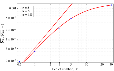
Figure 6: (Color online). Example of advanced fit (9) for a spheroid $r=5$, $k=5$. (Blue) dots – numerical data, solid (red) curve – fit by Eq. fit (9) with $B\approx 5.3\times 10^{-5}$, Pe${}_{1}\approx 5.2$ and Pe${}_{2}\approx 30.3$. Dashed (red) line is $B\,\mathrm{Pe}^{2}$. Here $\overline{\mathrm{Nu}}$ is the time-averaged Nu$(t)$ over the period of rotation (determined in the simulations), and $\overline{\mathrm{Nu}_{0}}$ is the time-averaged Nu$(t)$ for smallest available $\mathrm{Pe}$, e.g. $\mathrm{Pe}=0.01$.

IV Analytical model of heat transfer in a laminar shear flow

In this section we develop an analytical model for $\mathrm{Nu}(k,r,\varphi)$.

IV.1 Orientational statistics of elongated nano-particles

IV.1.1 Fokker-Plank equations for orientational PDF

In order to study the orientational statistics of elongated nano-particles we consider the Probability Distribution Function (PDF), $\mathcal{P}(\theta,\phi,t)$, which is the probability $P(\theta,\phi,t)$ of finding any particular spheroid with its axis of revolution in the interval $[\theta,\theta+d\theta]\times[\phi,\phi+d\phi]$ on the unit sphere. The PDF is then defined by

$$P(\theta,\phi,t)=\mathcal{P}(\theta,\phi,t)\sin\theta d\phi\,d\theta\ .$$ (12)

It was shown by Burgers Burgers1938 that $\mathcal{P}(\theta,\phi,t)$ satisfies a generalized Fokker-Planck equation in the presence of a shear:

$$\frac{\partial\cal P}{\partial t}=-\bm{\nabla}\cdot(\bm{w}\mathcal{P})+D_{r}\nabla^{2}\mathcal{P},$$ (13)

where $\bm{w}\equiv(0,\dot{\theta},\dot{\phi}\sin\theta)$ is the relative velocity on the unit sphere of the axis of revolution for a particle with instantaneous orientation $(\theta,\phi)$ ignoring all Brownian effects. The explicit form of this equation in spherical coordinates is:

$${\frac{\partial\mathcal{P}(\theta,\phi)}{\partial t}+\frac{1}{\sin\theta}\left[\frac{\partial}{\partial\theta}F_{\theta}\sin\theta+\frac{\partial}{\partial\phi}F_{\phi}\right]=0\ .}$$ (14a)

Here $$F_{\theta} F_{\phi} \theta \phi w D_{\rm{r}}$$ and , the and projections of the probability density fluxes that have two shear-induced contributions, one proportional to and the other to the rotational diffusion coefficient, :

$${{F_{\theta}=\Big{[}\frac{\partial\theta}{\partial t}-D_{\rm{r}}\frac{\partial}{\partial\theta}\Big{]}\mathcal{P}(\theta,\phi)\,,}}~{}~{}~{}~{}~{}~{}~{}~{}~{}~{}~{}$$ (14b)

$${{F_{\phi}=\big{[}\sin\theta\,\frac{\partial\phi}{\partial t}-\frac{D_{\rm{r}}}{\sin\theta}\,\frac{\partial}{\partial\phi}\big{]}\mathcal{P}(\theta,\phi)\ .}}$$ (14c)

Burgers in Ref. Burgers1938, derived the rotational diffusion coefficient, $D_{\rm{r}}$, of elongated rigid spheroids of revolution:

$$D_{\rm{r}} = \frac{k{{}_{{}_{\rm{B}}}}T}{4\mu V}\Big{[}\frac{r^{2}+1}{r^{2}K_{3}+K_{1}}\Big{]}^{-1}\ .$$ (15a)

Here $$\mu k{{}_{{}_{\rm{B}}}}=1.374\times 10^{-16} V=\frac{4}{3}\pi a^{2}b 2a=d b=ra r\geq 1$$ is the dynamical fluid viscosity, erg/deg K is the Boltsmann constant, particle volume , , , and

$$K_{3} = \int_{0}^{\infty}\frac{rdx}{(r^{2}+x)^{3/2}(1+x)}$$

$$= \frac{2}{r^{2}-1}\left[1-\frac{r\ \mathrm{arccosh}(r)}{\sqrt{r^{2}-1}}\right]\rightarrow 2\frac{\ln(2\,r/e)}{r^{2}}\,,$$

$$K_{1} = \int_{0}^{\infty}\frac{rdx}{(r^{2}+x)^{1/2}(1+x)^{2}}~{}~{}~{}~{}~{}~{}~{}~{}~{}~{}$$

$$= \frac{r}{r^{2}-1}\left[r-\frac{\mathrm{arccosh}(r)}{\sqrt{r^{2}-1}}\right]\rightarrow 1\ .$$

This asymptotics is formally valid for $r\gg 1$, but give better than 10% accuracy already for $r>4$, allowing us to suggest the approximate “practical” formula

$$D_{\rm{r}}\simeq\widetilde{D}_{\rm{r}}=\frac{k{{}_{{}_{\rm{B}}}}T}{4\mu V}\frac{\ln(4r^{2}/e)}{(r^{2}+2\,r/3-1)}\,,$$ (16)

that works with an accuracy of about $10\%$ for any $r\geq 1$ and better than with $5\%$-accuracy for $r>10$.

The complete analysis of Eqs. (14) is very involved, see e.g. Refs. Leal1971 and Hinch1972 . We consider only the small-diffusion limit, see the next subsection.

IV.1.2 Statistics of elongated nano-particles in the small diffusion limit

Jeffery Jef has shown that if inertial and Brownian motion affects are completely neglected, then the motion of the axis of revolution of a spheroidal particle is described by

$$\tan\phi = r\tan\tau\,,$$ (17a)

$$\tan{\theta} = C\sqrt{\cos^{2}\tau+r^{2}\sin^{2}\tau}$$

$$= C\,r\left(r^{2}\cos^{2}\phi+\sin^{2}\phi\right)^{-1/2},$$

where $\tau=t/T_{\rm r}$ with $T_{\rm r}=(r+1/r)/S$, and the constant of integration $C$ is called the (Jeffery) orbit constant.

To analyze the small-diffusion limit we introduce two time-scales. The first one defines the periodic motion that a nano-particle with a finite $r$ exhibits: $T_{\rm r}=T_{\rm J}/2\pi$, where $T_{\rm J}=2\pi(r+1/r)/S$ is the Jeffery’s period. The second time scale is determined by the inverse shear, $T_{S}=S^{-1}$. Clearly, for large $r$ this is a much shorter time scale, so for $r\gg 1$,

$$T_{r}\approx r/S=r\,T_{S}\ .$$ (18)

It means that the particles spend most of their time near pre- and post-aligned states. If the Brownian diffusion is small enough such that $T_{\rm dif}=D_{\mathrm{r}}^{-1}\gg T_{r}$ one can neglect the effect of the Brownian motion on the dynamic motions of particles along Jeffery orbits Jef even during their slow time evolution. In this case the stationary Fokker-Plank Eq. (13) takes the simple form

$$\bm{\nabla}\cdot(\bm{w}\mathcal{P})=0\ .$$ (19)

This equation can be solved Leal1971 ; Hinch1972 , giving

$$\mathcal{P}(\theta,\phi) = {f(C,r)}\,\mathcal{P}_{C}(\theta,\phi)\,,$$ (20a)

$$\mathcal{P}_{C}(\theta,\phi) = \left({\!r\,\sin\theta\cos^{2}\!\theta\sqrt{\cos^{2}\!\phi+\sin^{2}\!\phi/r^{2}\ }}\right)^{\!\!-1}\!\!\!,~{}~{}~{}~{}~{}~{}~{}$$ (20b)

where $\mathcal{P}_{C}(\theta,\phi)$ is the PDF along a particular Jeffery orbit with a given integration constant $C$, and ${f(C,r)}$ is the probability to occupy this orbit. This function is normalized as follows:

$$\int_{0}^{\infty}f(C)dC=\frac{1}{4\pi}\ .$$

${f(C,r)}$ was found in Leal1971 for the limiting cases:

$$f(C,r=1) = \frac{1}{4\pi}\frac{C}{(C^{2}+1)^{3/2}}\,,$$ (21a)

$$f(C,r\gg 1) \simeq \frac{1}{\pi}\frac{C}{(4C^{2}+1)^{3/2}}\,,$$ (21b)

$$f(C,r\ll 1) \simeq \frac{1}{\pi}\frac{Cr^{2}}{(4r^{2}C^{2}+1)^{3/2}}\ .$$ (21c)

Note that Eq. (21a) is exact, providing a consistency check of the present approach by comparison with spherical particles. The asymptotic, Eq. (21b), is very accurate for $r>20$, but already for $r\gtrsim 4$ it provides reasonable accuracy (better then $\sim 10\%$).

The analysis of Eqs. (21) together with the available numerical solutions for $r=0.26$ and $3.86$ Leal1971 allowed us to suggest the following approximation

$${{f(C,r)\simeq\frac{C/\!\left(r+1/r\right)^{2}}{\pi\left[1+4\,C^{2}/\!\left(r+1/r\right)^{2}\right]^{3/2}}}}\ .$$ (22)

A comparison of this approximation with the exact numerical solution provided in Ref. Leal1971 is presented in Fig. 7, upper panel. One sees that Eq. (22) fits the numerical data with an accuracy better than $5\%$. This is more then enough for our purpose to offer an approximate formula for $\langle\cos^{2}\theta_{\rm N}\rangle$ as a function of $r$, see below.

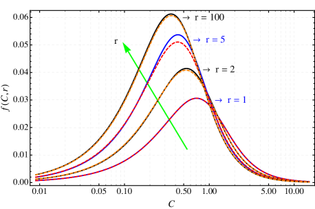
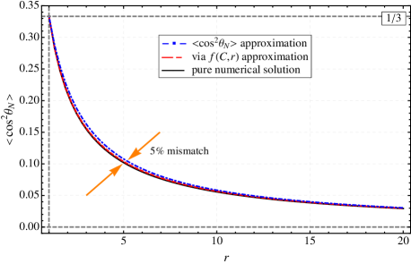
Figure 7: (Color online). Upper panel: Comparison of “exact numerical”, solutions, obtained from Eq. (19) (solid lines) and approximate solutions Eq. (22) for different $r$ (dashed lines). There is visible difference (about 5% in the value of maximum) only for $r=5$. Lower panel: Comparison of dependence of $\langle\cos^{2}\theta\rangle$ vs. $r$ obtained by a) applying “exact numerical” PDF (black solid line), b) approximate analytical PDF, Eq. (22), (red dashed line) and c) analytical approximation for this dependence Eq. (24) (blue dot-dashed line).

Next we use the fact that Jeffery orbits do not intersect on the unit sphere. In other words, fixing $C$ results in a relation between $\theta$ and $\phi$ along an orbit. This relationship is obtained by inverting Eq. (17):

$$C=C(\theta,\phi)=\tan\theta\sqrt{r^{-2}\sin^{2}\phi+\cos^{2}\phi}\ .$$ (23)

Substituting this function into any one of Eqs. (21) we get $f(C,r)$ for a given regime of $r$. This is then substituted in Eqs. (20), leading finally to a solution of the orientational PDF $\mathcal{P}(\theta,\phi)$, which can be used for averaging Eqs. (11) in the case of weak Brownian motions. As a consistency check of the approach one can consider the trivial case $r=1$. From Eq. (23) one finds $C=\tan\theta$, then from Rq. (21a) $f(C)=\sin\theta\cos^{2}\theta/4\pi$ and, finally from (20b) $\mathcal{P}_{C}=1/\sin\theta\cos^{2}\theta$. As the result one has for sphere $\mathcal{P}=1/4\pi$, as expected.

For moderate and strong Brownian rotational motion the notion of separate Jeffery orbits becomes irrelevant. In this case we need to solve Eq. (13) without approximations. Once this equation is solved we can compute $\langle\cos^{2}\theta\rangle$ and substitute the answer in Eqs. (11). To achieve this in the most general case is not a simple task, and here we satisfy ourselves with the two limiting cases of very large and very small rotational diffusion. The second case was discussed above. For the case of very strong rotational diffusion we can use the same Eqs. (11), but averaged with a uniform PDF $\mathcal{P}(\theta,\phi)=1/4\pi$. This is because the very strong rotational diffusion tends to distribute particles motions around the Jeffery orbits uniformly. The corrections up to $\mathcal{O}(S/D_{\mathrm{r}})^{2}$ to such a uniform distribution may be found in Ref. ML79 ; McMillen77

IV.2 Predictions of the model

IV.2.1 Spheroidal particle in a strong Brownian diffusion limit

With very strong Brownian diffusion, the particles are oriented completely randomly, and $\langle\cos^{2}\theta_{\mathrm{N}}\rangle=1/3$. In this case Eqs. (10) and (11) give the results reported in Fig. 8, upper panels. The upper left panel shows Nu vs. $r$ dependence for various $k$ from $1$ to $8600$ and $\infty$ with volume fraction $\varphi=1\%$. These results are rather obvious: for $k=1$ one obtains Nu$=1$, i.e. no enhancement; the larger the $k$, the larger the heat flux enhancement; for any finite $k$ there is a saturation of Nu$(r)$ for $r\to\infty$. The value of $($Nu$-1)$ may be huge for spheroids (essentially, rod-like particles at $r\gg 1)$, e.g. for $k=8600$ (diamond in water), Nu$-1\simeq 30$, while for spherical particles $(r=1)$, Nu$-1=0.03$ at the same volume fraction $\varphi=0.01$. The values of Nu$(k,r)$ are bounded, i.e. $\mathrm{Nu}(1,r)\leq\mathrm{Nu}(k,r)\leq\mathrm{Nu}(\infty,r)$.

The upper right panel shows Nu vs. $k$ dependence at $\varphi=1\%$ for three values of $r$: $1$, $5$ and $10$. The values of Nu$(k,r)$ are bounded, too: $\mathrm{Nu}(k,1)\leq\mathrm{Nu}(k,r)\leq\mathrm{Nu}(r,\infty)$. Here, the more elongated particle is (larger $r$), the better the enhancement.

And last, but not least: elongated particles may touch each other much easier. As we show in the Appendix B, the basic geometrical requirement that the mean inter-particle distance is less than the largest particle size means that $r<r_{0}\equiv\varphi^{-1/2}$, which is the basic criteria of the dilute limit. The Nu$(r)$ dependence for $r<r_{0}$ is shown by solid curves, while the region $r>r_{0}$ is shown by dashed curves in Figs. 8, left panels. Provided, $r\leq 10$ at $\varphi=1\%$, the enhancement may be still considered as large but not huge: for $k=5$, the saturation level of (Nu-1) is about $0.25$ while for spheres Nu$-1\approx 0.017$.

The conclusion in the case of very strong Brownian diffusion is that the particles with larger $k$ and $r$ bring larger heat flux enhancement in the laminar shear flow.

IV.2.2 Spheroidal particle in a weak Brownian diffusion limit

To complete the calculations of Nu$(r)$ dependence in a weak Brownian diffusion limit in the framework of model (11), we have to find $\langle\cos^{2}\theta_{\mathrm{N}}\rangle$ vs. $r$. To make a long story short, we compared in Fig. 7, lower panel, the dependence of $\langle\cos^{2}\theta_{\mathrm{N}}\rangle$ vs. $r$ obtained by numerically solved PDF, Eq. (19) (see Refs. Leal1971 ; Hinch1972 for more details), shown by (black) solid curve, and by approximate analytical PDF, Eq. (22), shown by (red) dashed curve. As one sees these two dependence coincide within line width. Moreover, by careful analysis of various limiting cases, we suggested the following simple model dependence

$${\langle\cos^{2}\theta_{\mathrm{N}}\rangle\simeq\frac{2}{6+\pi\,(r-1)}\,,}$$ (24)

shown in Fig. 7, lower panel, as a (blue) dash-dotted curve. Eq. (24) fits the exact dependence with an accuracy of 5%. Therefore, Eqs. (11) and (24) can be used in our analysis to make predictions on the thermal properties in the limit of small Brownian diffusion of fluids laden with spheroidal nano-particles of different aspect ratios and different thermal conductivity ratios with Peclet number up to unity. Corresponding results are shown in Fig. 8, lower panels.

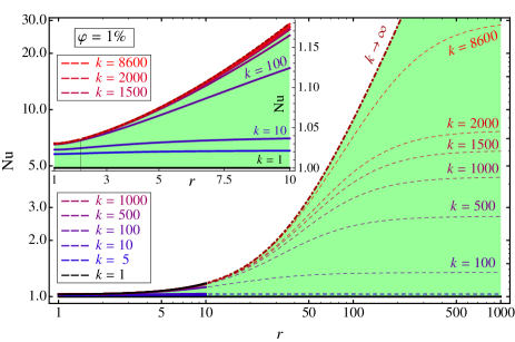
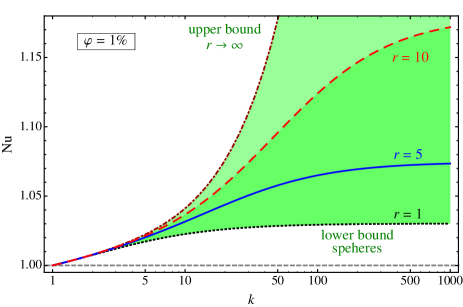
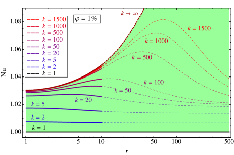
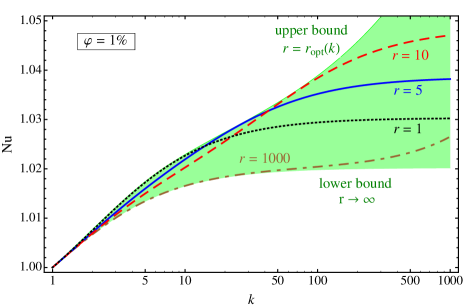
Figure 8: (Color online). $\varphi=1\%$, $r_{0}=10$. Upper panels: Strong Brownian diffusion limit: $\left\langle\cos^{2}\theta_{\mathrm{N}}\right\rangle\rightarrow 1/3$, lower panels: Weak Brownian diffusion limit. Left panels: Nusselt number, Nu, vs. particle aspect ratio, $r$, for various heat diffusivity ratios, $k$: solid curves for $r<r_{0}$, dashed curves for $r>r_{0}$ (the region, where the particles may, in principle, start touching each other). The shaded (green) area is the region of all possible Nu$(k,r)$ at $\varphi=0.01$: the lower bound is given by Nu$(1,r)$, the upper one is Nu$(\infty,r)$. Right panels: Nu vs. $k$ for various, $r$. Dotted (black) curve is for $r=1$, spherical particles, solid (blue) curve – $r=5$, dashed (red) curve – $r=10$, and dot-dashed (brown) curve – $r=1000$, lower panel, or $r\to\infty$, upper panel. The shaded (green) area is the region of all possible Nu$(k,r)$ at $\varphi=0.01$: the lower bound is Nu$[k,1]$ in upper panel and Nu$(k,\infty)$ in lower panel, while the upper bound is Nu$(k,\infty)$ in upper panel and Nu$[k,r_{\mathrm{opt}}(k)]$ in lower panel, where $r_{\mathrm{opt}}(k)$ maximizes Nu at every $k$, see more in the text. The geometrical constrain imposes $1\leq r\leq\max(r_{\mathrm{opt}},10)$ for $\varphi=1\%$.

The lower left panel in Fig. 8 shows Nu$(r)$ for different $k$ and $\varphi=0.01$, at which the Maxwell-Garnett limit of Nu$-1$ for spherical particles ($r=1$) is $3\varphi=0.03$. Notice, the Nu$(r)$ dependence is not monotonic and has a maximum at some $r=r_{\mathrm{opt}}$, which depends on $k$. The reason for this is the competition of two effects: more elongated nano-particles give larger contribution to the heat flux when their longer axis is aligned with the temperature gradient, which is orthogonal to the velocity gradient (shear) in our case. However longer nano-particles are affected more readily by the shear, which tends to orient them in the unfavorable direction orthogonal to the temperature gradient; then their contribution to the heat flux is even less than the one of the spherical particles (cf. Fig. 5). Again, the values of Nu$(k,r)$ are bounded, i.e. $\mathrm{Nu}(1,r)\leq\mathrm{Nu}(k,r)\leq\mathrm{Nu}(\infty,r)$.

The lower right panel in Fig. 8 shows Nu$(k)$ for different aspect ratios, $r$ at $\varphi=1\%$. This is again a consequence of the above described competition. The values of Nu are bounded by $\mathrm{Nu}(k,\infty)\leq\mathrm{Nu}(k,r)\leq\mathrm{Nu}[k,r_{\mathrm{opt}}(k)]$. Moreover, for $1\leq k\lesssim 7$ the optimal nano-particle shape is spherical.

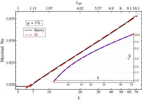
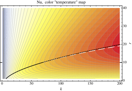
Figure 9: (Color online). Weak Brownian diffusion limit, $\varphi=1\%$, $r_{0}=10$. Left: The largest reachable Nusselt number, $\mathrm{Nu}(k,r_{\mathrm{opt}})$, solid (black) curve ($r_{\mathrm{opt}}$ maximizes Nu for a given $k$). Dashed (red) line is the fit by $\mathrm{Nu}_{\mathrm{max}}^{\mathrm{fit}}\approx 1+\varphi[0.75+0.66\ln(k)]$. Insert: $r_{\mathrm{opt}}$ vs. $k$, solid (blue) curve, and the fit $r_{\mathrm{opt}}^{\mathrm{fit}}\approx-3.03+1.57\sqrt{k}$ for $1\leq r_{\mathrm{opt}}\leq 10$, dashed (red) line. Since $\varphi=0.01\ll 1$, this fit may be considered as $\varphi$-independent for $\varphi\leq 1\%$. Right: Contour-density plot of Nu$(k,r)$ color-codded with the “temperature” map: the larger the value of Nu, the wormer the color; contours show iso-values of Nu. Thick (black) solid and dashed curves represent those pairs of $(k,r)$ for which Nu is maximal (i.e. solid (blue) curve in the Insert); solid curve is for $r<r_{0}$, and the dashed one is for $r>r_{0}$. Wide-dash (white) curve is the $r_{\mathrm{opt}}^{\mathrm{fit}}(k)$ fit.

As seen in Fig. 8, lower left panel, there exists a maximum of Nu$(r=r_{\mathrm{opt}})$ for a given $k$. This maximal Nusselt number at its maximizing (optimal) $r=r_{\mathrm{opt}}(k)$ is shown in Fig. 9, left, as a function of $k$ for $\varphi=0.01$. For $k>7$, the maximal Nu behaves like

$$\mathrm{Nu}_{\mathrm{max}}^{\mathrm{fit}}\approx 1+\varphi\left[0.75+0.66\ln(k)\right],\ \ \varphi=0.01\ .$$ (25a)

Since here $$\varphi\ll 1 \varphi \varphi\leq 1\%$$, the part in parenthesis may be considered as -independent, thus, the fit (25a) may be used at any .

The right panel of Fig. 9 exhibits a contour-density plot of Nu$(r,k)$ at $\varphi=0.01$. Thick (black) solid and dashed curves show $r_{\mathrm{opt}}(k)$ dependence (solid curve is for $r<r_{0}$, and the dashed one is for $r>r_{0}=\varphi^{-1/2}=10$). The inverse dependence $k(r_{\mathrm{opt}})$ is easy to obtain in a symbolic computation software by solving $\partial$Nu$(r,k,\varphi)/\partial r=\partial\mathcal{K}(r,k,\varphi)/\partial r=0$ at $r=r_{\mathrm{opt}}$, though, the answer appears to be very cumbersome to be shown here. However, our analysis reveals that $r_{\mathrm{opt}}\sim\sqrt{k}$, and for $\varphi=0.01$ and $1\leq r_{\mathrm{opt}}\leq 10$, .

$$r_{\mathrm{opt}}^{\mathrm{fit}}(k)\approx-3.03+1.57\sqrt{k}\,,\quad\varphi=0.01\ .$$ (25b)

This dependence is shown in Fig. 9, right, as a wide-dashed (white) curve, which deviates from the analytical solution $r_{\mathrm{opt}}(k)$ for $r_{\mathrm{opt}}>10$. Again, since $\varphi\ll 1$, the fit (25b) may be used at any $\varphi\leq 1\%$.

In conclusion, we should notice that the rich information about heat flux enhancement, shown in the four panels of Fig. 8, is just an illustration of the analytical dependence Nu$(\varphi,k,r)$ given by the analytical expressions (11) and (24). This is an important result of our modeling.

CONCLUSIONS

We presented a study of the physics of the heat flux in a fluid laden with nanoparticles of different physical properties (shape, thermal conductivity, etc). We developed a new analytical model for the effective thermal properties of dilute nanofluid suspensions. Our model accounts for nanoparticle rotation dynamics including the fluid motion around the nanoparticles. We note that our model reproduces the classical Maxwell-Garnet model in the appropriate static limits.

We used a combination of theoretical models and numerical experiments in order to make progress from the simplest case of spherical nanoparticles in a quiescent fluid to the most general case of rotating spheroidal particles in shear flows. The new physical ingredient that we consider is the exact dynamics of particles in shear flows. This constitute a novelty as most of the models introduced so far, to explain the thermal properties of thermal colloids, have focused only on the static properties of the nanoparticle suspension. Our model starts from the realization that particles (spherical or spheroidal) in the presence of a gradient of the velocity field are induced to rotate. The dynamics of rotation is absolutely non trivial, but it has been studied at length with correspondece (for the case of a laminar and stationary shear flow) to the Jeffery orbits.

The particles rotation dynamics has a double influence on the thermal properties of the nanofluid. First, particles rotation induces fluid motions in the proximity of the particles, this in turn can enhance the thermal fluxes by means of advective motions along the direction of the temperature gradient. Second, the Jeffery dynamics of particles leads to a statistical distribution of particles orientation that depends on a multitude of parameters, e.g. the particle aspect ratio, the shear intensity as well as on the intensity of thermal fluctuations. The statistical distribution of particle orientation has a dramatic influence on the heat flux: an elongated particle oriented along the temperature gradient increases the thermal flux, while a particle with perpendicular orientation reduces it.

The statistical orientation of particles can thus produce a mixed effects with a non-trivial dependence on the particle aspect ratio. More Elongated particles can enhance the heat flux because of the stronger contribution when properly aligned to the temperature gradient but, because of shear, more elongated particles are also spending more time in the unfavorable direction (i.e. perpendicular to the temperature flux) thus reducing the thermal conductivity of the fluid.

By means of numerical approximations we are able to provide closed expressions for the effective conductivity of the fluid under several flow regimes and for several physical parameters. Our model considerably extends classical models for nanofluid heat transfer, like e.g. the one of Maxwell-Garnet, and may help to rationalize some of the recent experimental findings. In particular, we suggest that experiments should consider more carefully measurements performed in quiescent and under flowing conditions: the particles dynamics may lead to very different thermal properties in the two cases.

Finally, the next steps toward a robust predictive models for the heat transfer in nanofluids should include the effect of surface (Kapitza) resistance and the effect of nanoparticle aggregation. Further it would also be extremely important to extend the model to the case of heat flux in turbulent nanofluids as this case is very relevant to many applications. In the presence of turbulence a particular attention should also be paid to the effect on the drag induced by the presence of spherical, rod-like or maybe even deformable nanoparticle inclusions.

Appendix A Numerical approach

The numerical simulation of the conjugated heat transfer problem, equations (4a-4c), is performed by means of two coupled D3Q19 Lattice Boltzmann (LB) equations under the BGK approximation Succi2001 (for velocity and temperature fields) and Molecular-Dynamics simulations (for particles motion):

$$f_{l}({\bm{x}}+{\bm{c}}_{l},t+1)-f_{l}({\bm{x}},t)= \dfrac{f_{l}^{\rm eq}({\bm{x}},t)-f_{l}({\bm{x}},t)}{\tau_{\rm f}}\,,~{}~{}~{}~{}$$ (26a)

$$g_{l}({\bm{x}}+{\bm{c}}_{l},t+1)-g_{l}({\bm{x}},t)= \dfrac{g_{l}^{\rm eq}({\bm{x}},t)-g_{l}({\bm{x}},t)}{\tau_{\rm g}}\,,~{}~{}~{}~{}$$ (26b)

where $f_{l}({\bm{x}},t)$ is the Lattice Boltzmann distribution function for particles at $({\bm{x}},t)$ with velocity ${\bm{c}}_{l}$ (with $l={0,\dots,18}$ for D3Q19), and $f_{l}^{\rm eq}$ is its equilibrium distribution; $g_{l}({\bm{x}},t)$ is the distribution functions associated with the temperature and $g_{l}^{\rm eq}$ is its equilibrium distribution. The first LB, Eq. (26a), evolves the fluid flow outside of the rigid particle and its momentum is coupled with the particle boundaries by means of a standard scheme, as proposed by Ladd Ladd2006 . The second LB, Eq. (26b), evolves the temperature field, treated as a passive scalar as proposed in Chen1998 , solving the conjugated heat transfer problem simply by means of adjusting the thermal conductivity to the correct values in the fluid and inside the particle [eqn. (4a) and (4b)]. Thermal and velocity boundary conditions, at the top and bottom walls, impose the LB populations to equal the equilibrium populations (corresponding to the desired velocity and temperature). This approach can produce small temperature and velocity slip which are kept into account by measuring the effective temperature and velocity profiles, thus increasing the accuracy. The code employed is fully parallelized by means of MPI libraries MPI thus allowing large system sizes, important to study the influence of finite size effects.

Density, momentum and temperature are defined locally at $({\bm{x}},t)$ as coarse-grained (in velocity space) fields of the distribution functions

$$\rho_{\rm f}=\sum_{l}f_{l}\,,\hskip 14.45377pt\rho_{\rm f}{\bm{u}_{\rm f}}=\sum_{l}{\bm{c}}_{l}f_{l}\,,\hskip 14.45377pt\rho_{\rm f}T_{\rm f}=\sum_{l}g_{l}\ .~{}~{}~{}~{}~{}$$ (27)

A Chapman-Enskog expansion Guo2 around the local equilibria $f^{\rm eq}_{l}({\bm{u}},\rho)$ and $g^{\rm eq}_{l}({\bm{u}},T)$ Guo1 leads to the equations for temperature and momentum (4a)-(4b): the streaming step on the left hand side of (26a) reproduces the inertial terms in the hydrodynamical equations, whereas the diffusive terms (dissipation and thermal diffusion) are closely connected to the relaxation (towards equilibrium) properties in the right hand side, with $\nu$ and $\chi$ related to the relaxation times $\tau_{\rm f}$, $\tau_{\rm g}$ Succi2001 .

A.0.1 Conjugated heat transfer for a spherical particle at rest

Consider a spherical particle of radius $R$ immersed in a quiescent fluid, in which a constant temperature gradient, $\bm{G}$, is maintained. The temperature distribution is LnL :

$$T_{\rm{p}}(\bm{r}) = \frac{3}{2+k}\bm{G}\cdot\bm{\rho}\,,\qquad\qquad\qquad\ \ \,r<R\,,$$ (28)

$$T_{\rm{f}}(\bm{r}) = \left[1+\frac{1-k}{2+k}\left(\frac{R}{\rho}\right)^{\!3}\right]\bm{G}\cdot\bm{\rho}\,,\quad r\geq R\,,$$

where $\rho=\sqrt{x^{2}+y^{2}+z^{2}}$ is the distance from the particle’s center.

In our Couette flow simulations, $\bm{G}={\widehat{\bf{y}}}\,\Delta/H$, but the temperature boundary conditions are different from LnL . One should expect then deviations close to the walls especially for large particles. The results are presented in Fig. 2.

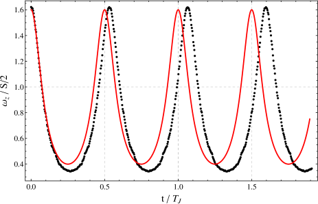
Figure 10: Angular velocity vs. time. Solid (red) curve – theory of Jeffery Jef , Eqs. (29), for an infinite domain with a constant simple shear at infinity and the creeping (Re$\rightarrow 0$) flow around the particle, dots – numerical results for small but finite Re$=0.05$. Configuration: $64^{3}$, Pr $=10$, $k=1$, $r=2$ ($a=14$, $b=7$), Pe $=0.5$.

A.0.2 Spheroid in a shear flow – “Jeffery” test

A spheroidal particle of aspect ratio $r$ in a simple shear flow undergoes a spinning motion (in the $XY$-plane). The angular velocity and the period of such a motion were predicted by Jeffery Jef for a case of a creeping flow around the particle, i.e. when Re$\rightarrow 0$:

$$\omega_{z} = \frac{S\,r/\!\left(r+1/r\right)}{\cos^{2}\!\left(2\pi\,t/T_{\rm J}\right)+r^{2}\sin^{2}\!\left(2\pi\,t/T_{\rm J}\right)}\,,~{}~{}~{}~{}$$ (29a)

$$T_{\rm J} = {2\pi}\left(r+{1}/{r}\right)/{S}\ .$$ (29b)

For non-vanishing Re, the actual period of rotation of the particle deviates from that predicted by Jeffery. In Fig. 10 we compare the results of our LBM simulations with Eq. (29a) for the case of $r=2$ and Re$=0.05$. There is a 6% difference in periods due to a finite Re, but also due to influence of the other particles present due to the periodic b.c., and also the influence of the walls ($2a/H\simeq 0.44$).

Appendix B Approximation of non-interacting particles

The approximation of non-interacting spheroids is comming from simple geometrical considerations, and it is valid provided the particle aspect ratio $r<\varphi^{-1/2}$, as confirmed by the following derivation:

$$\varphi = \frac{V_{\rm{\rm all\,paricles}}}{V_{\rm total}}=\frac{N\,V_{\rm particle}}{V_{\rm total}}=\frac{V_{\rm particle}}{V_{\rm eff}}$$

$$= \frac{4\pi\,a\,b^{2}/3}{V_{\rm eff}}=\frac{4\pi\,a\,b^{2}/3}{\mathcal{L}^{3}}=\frac{4\pi\,a^{3}\,r^{-2}/3}{\mathcal{L}^{3}}\quad\Rightarrow$$

$$\mathcal{L} = \sqrt[3]{\frac{4\pi\,a^{3}\,r^{-2}/3}{\varphi}}=a\sqrt[3]{\frac{4\pi}{3\,r^{2}\varphi}}\,,$$

$$2a < \mathcal{L}\quad\Rightarrow\quad r<\sqrt{\frac{\pi}{3\varphi}}\quad\Rightarrow\quad r<\varphi^{-1/2}.$$ (30)

Here $N$ is the number of particles in the total volume (of fluid and particles together), $V_{\mathrm{total}}$, $V_{\mathrm{eff}}=V_{\mathrm{total}}/N$ is an “effective” volume per particle, and $\mathcal{L}=V_{\mathrm{eff}}^{1/3}$ is a characteristic length/dimension of the effective box/volume embedding the particle.

References

- (1) Jing Fan and Liqiu Wang, “Review of Heat Conduction in Nanofluids”, J. Heat Transfer 133, 040801 (2011)
- (2) Clement Kleinstreuer and Yu Feng, “Experimental and theoretical studies of nanofluid thermal conductivity enhancement: A review”, Nanoscale Research Letters 6, 229 (2011).
- (3) J.H. Lee, S.H. Lee, C.J. Choi, S.P. Jang, and S.U.S. Choi, “A Review of Thermal Conductivity Data, Mechanisms and Models for Nanofluids”, International Journal of Micro-Nano Scale Transport 1, 269 (2010).
- (4) Jacopo Buongiorno, David C. Venerus, Naveen Prabhat, Thomas McKrell, Jessica Townsend, Rebecca Christianson, Yuriy V. Tolmachev, Pawel Keblinski, Lin-wen Hu, Jorge L. Alvarado, In Cheol Bang, Sandra W. Bishnoi, Marco Bonetti, Frank Botz, Anselmo Cecere, Yun Chang, Gang Chen, Haisheng Chen, Sung Jae Chung, Minking K. Chyu, Sarit K. Das, Roberto Di Paola, Yulong Ding, Frank Dubois, Grzegorz Dzido, Jacob Eapen, Werner Escher, Denis Funfschilling, Quentin Galand, Jinwei Gao, Patricia E. Gharagozloo, Kenneth E. Goodson, Jorge Gustavo Gutierrez, Haiping Hong, Mark Horton, Kyo Sik Hwang, Carlo S. Iorio, Seok Pil Jang, Andrzej B. Jarzebski, Yiran Jiang, Liwen Jin, Stephan Kabelac, Aravind Kamath, Mark a. Kedzierski, Lim Geok Kieng, Chongyoup Kim, Ji-Hyun Kim, Seokwon Kim, Seung Hyun Lee, Kai Choong Leong, Indranil Manna, Bruno Michel, Rui Ni, Hrishikesh E. Patel, John Philip, Dimos Poulikakos, Cecile Reynaud, Raffaele Savino, Pawan K. Singh, Pengxiang Song, Thirumalachari Sundararajan, Elena Timofeeva, Todd Tritcak, Aleksandr N. Turanov, Stefan Van Vaerenbergh, Dongsheng Wen, Sanjeeva Witharana, Chun Yang, Wei-Hsun Yeh, Xiao-Zheng Zhao, and Sheng-Qi Zhou, “A benchmark study on the thermal conductivity of nanofluids”, Journal of Applied Physics 106, 094312 (2009).
- (5) Sezer Ozerinc, Sadik Kakac and Almila Guvenc Yazicioglu, “Enhanced thermal conductivity of nanofluids: A state-of-the-art review”, Microfluidics and Nanofluidics 8, 145 (2009).
- (6) J. A. Eastman, U. S. Choi, S. Li, L. J. Thompson, and S. Lee, “Enhanced thermal conductivity of through the development of nanofluids”, 1996 Fall Meeting of the Materials Research Society, Boston, 2–6 Dec. 1996 (MRS, Pittsburgh, 1996), p.1.
- (7) S. Kabelac and J. F. Kuhnke, “Heat transfer mechanisms in nanofluids: Experiments and theory”, Annals of the Assembly for International Heat Transfer Conference 13, KN (2006).
- (8) Ce-Wen Nan, R. Birringer, David R. Clarke, and H. Gleiter, “Effective thermal conductivity of particulate composites with interfacial thermal resistance”, Journal of Applied Physics 81, 6692 (1997).
- (9) G. B. Jeffery, The Motion of Ellipsoidal Particles Immnersed in a Viscous Fluid, Proc. Roy. Soc. London, Ser. A 102, 161 (1922).
- (10) L.G. Leal and E.J. Hinch, The effect of weak Brownian rotations on particles in shear flow, Journal of Fluid Mechanics 46, 685 (1971).
- (11) E.J. Hinch and L.G. Leal, The effect of Brownian motion on the rheological properties of a suspension of non-spherical particles, Journal of Fluid Mechanics 52, 683 (1972).
- (12) M.P. Allen and D.J. Tildesley, Computer Simulation of Liquids (Oxford University Press, Oxford, 1987).
- (13) S. Succi, The Lattice Boltzmann Equation for Fluid Dynamics and Beyond (Numerical Mathematics and Scientific Computation) (p. 304). Oxford University Press, USA, (2001).
- (14) Landau, L.D. and Lifshitz, E.M. A Course in Theoretical Physics-Fluid Mechanics, Pergamon Press Ltd. (1987).
- (15) Jeffrey, D. J., Proc. R. Soe. London Set. A. 335 (1973), 338, 503 (1974).
- (16) Chiew and Glandt. Effective conductivity of dispersions: The effect of resistance at the particle surfaces. Chemical Engineering Science 42, 2677-2685 (1987).
- (17) Maxwell, J. C., ”Electricity and Magnetism,” 1st ed., p. 365. Oxford Univ. Press, (Clarendon), London, 1973.
- (18) Eastman, J.a., S.R. Phillpot, S.U.S. Choi, and P. Keblinski. ”Thermal Transport in nonofluids”, Annual Review of Materials Research 34, 219-246 (2004).
- (19) J.M. Burgers. In Second Report on Viscosity and Plasticity, chapter 3. Kon. Ned. Akacl. Wet. Verhand. (Eerste Sectie) 16, 113, (1938).
- (20) T. J. Mcmillen 1 and L. G. Leal, The Bulk Heat Flux for a Sheared Suspension of Prolate Spheroids at Low Particle Peclet Number Journal of Colloid and lnterJace Science, 69, 45-67 (1979)
- (21) Thomas Joe McMillen, The thermal constitutive behavior of suspensions, PhD Thesis, CalTech, Pasadena, CA (1977). Direct calculation of the velocity field around nanoparticle in terms of the spherical harmonics, Eq.(16), p. 108
- (22) A.J.C. Ladd, Numerical simulations of particulate suspensions via a discretized Boltzmann equation. Part 1. Theoretical foundation. Journal of Fluid Mechanics 271, 285–309 (2006).
- (23) He, X., Chen, S., & Doolen, G., A novel thermal model for the lattice Boltzmann method in incompressible limit. J. Computational Physics 146, 282-300 (1998).
- (24) http://en.wikipedia.org/wiki/Message_Passing_Interface
- (25) Z. Guo, C. Zheng & B. Shi, Phys. Rev. E 65, 046308 (2002)
- (26) Z. Guo, Z., B. Shi, T. S. Zhao, & C. Zheng, Phys. Rev. E 76, 056704 (2007)