Phase Transition in a Bond Fluctuating Lattice Polymer

Hima Bindu Kolli
and
K.P.N.Murthy

School of Physics, University of Hyderabad
Hyderabad 500046
November 2011

ABSTRACT

This report deals with phase transition in Bond Fluctuation Model (BFM) of a linear homo polymer on a two dimensional square lattice. Each monomer occupies a unit cell of four lattice sites. The condition that a lattice site can at best be a part of only one monomer ensures self avoidance and models excluded volume effect. We have simulated polymers with number of monomers ranging from $10$ to $50$ employing Boltzmann and non-Boltzmann Monte Carlo simulation techniques. To detect and characterize phase transition we have investigated heat capacity through energy fluctuations, Landau free energy profiles and Binder’s fourth cumulant. We have investigated (1) free standing polymer (2) polymer in the presence of of an attracting wall and (3) polymer confined between two attracting walls. In general we find there are two transitions as we cool the system. The first occurs at relatively higher temperature. The polymer goes from an extended coil to a collapsed globule conformation. This we call collapse transition. We find that this transition is first order. The second occurs at a lower temperature in which the polymer goes from a collapsed phase to a very compact crystalline phase. This transition is also discontinuous. We find that in the presence of wall(s) the collapse transition occurs at lower temperature compared to a free standing polymer.

Chapter 1 INTRODUCTION

1.1 Polymers

A polymer is a long chain of several simple atomic groupings called monomers. These monomers are held together by chemical bonds [1]. The process of forming a long chain of monomers is called polymerization. The number of monomers in a polymer is denoted by $N$ and is called the degree of polymerization. If the available bonds for a monomer are two, then the process of polymerization leads to a linear polymer. If the available bonds are more than two, then it leads to a branched and cross linked polymer. A polymer with same type of monomers is called a homopolymer and that with different types of monomers is called a heteropolymer. In this report we shall deal with a linear homopolymer.

1.2 Solvent and Temperature Effect

A polymer can exist in several conformations [2]. The conformation has a direct bearing on its physical properties. The conformational statistics of a polymer chain depends on the solvent quality. For a good solvent, interactions between monomers and solvent molecules are more favourable than interaction between non-bonded monomers. Hence in a good solvent, polymer segments would prefer to be surrounded by the solvent, leading to a swollen coil conformation. We call this as extended phase. For a bad solvent, the interaction between non-bonded monomers are more favourable leading to a compact globule conformation. We call this as collapsed phase. A good parameter that quantifies the size of the polymer is the radius of gyration or end-to-end distance. This quantity will be relatively large for extended conformation and small for collapsed conformations

The quality of solvent is often parameterized by temperature. Low temperatures correspond to a poor solvent and high temperatures correspond to a good solvent. As the temperature decreases, a transition occurs from an extended coil phase to collapsed globule phase. At very low temperatures, another transition from globular phase to crystalline phase takes place if the cooling rate is slow. Upon fast cooling glass formation becomes possible at these low temperatures.

Coarse grained models are often employed in polymer studies. A coarse grained model, see e.g. [3, 4, 5], treats a group of chemical monomers as a bead (effective monomer) ignoring the microscopic degrees of freedom, which are invariably present; it retains only the most basic features common to all polymers of the same chain topology. Such a model incorporates features such as chain connectivity, excluded volume effect and monomer-monomer interactions.

In this work we consider lattice model of a linear homopolymer. For an introduction to lattice models of polymers, see e.g [3]. We restrict our attention to a polymer on a two dimensional square lattice. The trail of a self avoiding random walk provides a model of a polymer conformation. In this section, we give a brief description of random walk (RW), self avoiding walk (SAW) and Interacting self avoiding walk (ISAW).

1.3 Random Walk

A random walk starts from an arbitrary lattice point which is taken as origin. It selects one of the four nearest neighbour sites randomly and with equal probabilities and steps into it. This process is iterated and we get a random walk of desired length. Thus a simple random walk generates a chain that can intersect as well as fold on to itself. Fig. (1.1) shows a random walk of 22 steps.

In a polymer, we have the so-called excluded volume effect. This is also known as hard core repulsion. In a lattice model, the excluded volume effect can be easily implemented by demanding that a lattice site can at best be occupied by a single monomer. This leads us to self avoiding random walk.

1.4 Self Avoiding Walk (SAW)

A self avoiding walk is a random walk that does not visit a lattice site it has already visited. A self avoiding walk [6] is an athermal walk. A self avoiding walk models a polymer at very high temperatures where segment-segment interactions are negligible. With lowering of temperature, the segment - segment interaction comes into play. To model segment - segment interaction we consider Interacting Self Avoiding Walk (ISAW) [7].

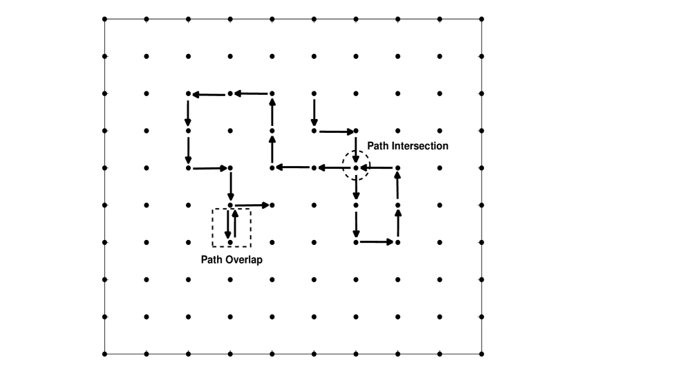
Figure 1.1: A simple random walk of $22$ steps involving intersections and overlaps of the path.

1.5 Interacting Self Avoiding Walk (ISAW)

We assign an energy $\epsilon$ to every pair of occupied nearest-neighbour sites which are not adjacent along the walk. Such a non-bonded nearest- neighbour (nbNN) pair gives rise to an nbNN contact or simply a contact. If $\epsilon\ <\ 0$ the interaction is attractive. If $\epsilon\ >\ 0$ the interaction is repulsive. Thus a conformation with $m$ contacts has energy $E=m\epsilon$. A SAW with energy assigned in this fashion is called an Interacting Self Avoiding Walk (ISAW). A typical ISAW on a square lattice of walk length $N=26$ with total number of nbNN contacts $m=6$ is shown in Fig. (1.2). In this work, our aim is to study phase transition from an extended to a collapsed phase. Hence we take $\epsilon$ to be negative. Without loss of generality we set $\epsilon=-1$. In other words we measure energy in units of $\epsilon$

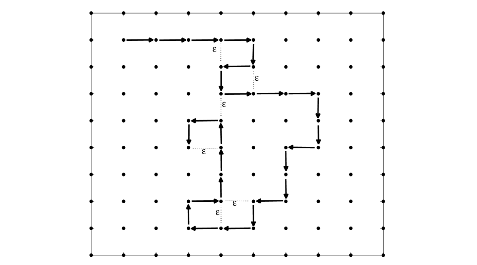
Figure 1.2: A interacting Self Avoiding walk (ISAW) that models a lattice polymer having $27$ monomers. Two monomers on nearest neighbour lattice sites but not connected by a bond constitute a non bonded Nearest Neighbour (nbNN) contact pair or simply a contact. The contacts are indicated by dotted lines.

1.6 Algorithms to generate ISAW

In the study of lattice polymers employing self avoiding walks three approaches have so far been tried out. The first is called stochastic growth algorithms which include kinetic growth walks. The second is based on the method proposed by Sokal involving local changes in a fully grown polymer. The third is called Bond Fluctuation Model (BFM). We discuss the first two approaches briefly below. The third model is discussed in detail in the next chapter.

1.6.1 Growth algorithm

An early stochastic growth method on a lattice employed a blind ant algorithm, where the ant moves blindly to one of the nearest neighbour sites with equal probability. At any growth step, if the selected site is already occupied by a monomer then we discard the whole walk and start all over again. This ensures that all the random walks are generated with equal probability given by $(1/4)\times(1/3)^{N-1}$, where $N$ is the number of steps in the walk. Notice that an $N$-step walk generates a polymer with $N+1$ monomers. From the lattice polymers generated by the blind ant, we can construct micro canonical ensembles by grouping then in terms of energies; we can also carry out canonical ensemble averages by attaching a Boltzmann weight to each walk based on its energy. A major problem with blind ant is sample attrition i.e., only a small fraction of starting chains are finally accepted. Most of the walks overlap or intersect before reaching the required chain length; in other words the walks get terminated early most of the time. This is called the problem of sample attrition. Longer the walk, the more is the problem posed by attrition. Partial remedy is Rosenbluth - Rosenbluth (RR) walk based on myopic ant [8]. The ant selects one of the unoccupied nearest neighbour sites randomly and with equal probability. Sample attrition is considerably reduced, though not eliminated. Trapping does still occur.

A major problem with a myopic ant is the following. The walks generated are not all equally probable. Hence we need Rosenbluth Rosenbluth (RR) weights, $W_{RR}$ for calculating micro canonical ensemble averages. We need RR weights as well as Boltzmann weights, see below, for calculating canonical ensemble averages. RR weight usually fluctuates wildly from one walk to the other. Besides sample attrition is present, though less; hence long walks remain difficult to generate.

Kinetic Growth walks (KGW) [9] are RR walks, where, we ignore RR weights. The justification is that we are looking at a polymer that grows faster than it could relax. KGW has been shown to belong to the same universality class as SAW [10]. More recently KGW has been generalized where one selects the available unoccupied sites on the basis of the number of contacts it would establish [11, 12]. For example if the move would increase the contacts by one then the local Boltzmann weight for that move is $\exp(-\beta)$. The site for placing the monomer is selected on the basis of probability constructed from the local Boltzmann weights. This is called Interacting Growth walk (IGW) and has been shown to belong to same universality class as ISAW [11].

Grassberger [13] has proposed PERM algorithms to extract equilibrium properties from KGW ensembles. Ponmurugan et al [14] have proposed flat-IGW algorithm to calculate equilibrium averages from IGW ensembles. Thus kinetic and interacting growth walks have proved useful in polymer studies.

1.6.2 Sokal algorithm

The second approach is provided by A D Sokal [15]. We start with a lattice polymer of a given length. We make local changes employing moves like pivoting about a chosen monomer, cranking, rotating about an axis etc. in a self avoiding fashion to generate a trial configuration. Figs. (1.3, 1.4) depict some possible moves. We employ standard Metropolis algorithm to accept/reject the trial configuration. We generate a Markov chain of polymer conformations and the asymptotic part of the Markov chain corresponds to a canonical ensemble.

We calculate the desired properties by averaging over the canonical ensemble. A problem with Sokal’s algorithm is that local changes are often difficult to make and time consuming especially for long polymers.

1.6.3 Bond Fluctuation Model

The third approach is the bond fluctuating model [16]. It combines the advantages of both the growth and the Sokal algorithms. In this model we start with a possible polymer conformation of desired length like in Sokal’s algorithm. Hence there is no problem of sample attrition. A monomer is chosen and moved to its nearest neighbour site in a self avoiding way. The move is thus simple and local, like in growth algorithm. In this model, however, the bond length fluctuates. Since bond fluctuation model forms the backbone of this work, it is described separately and in details in next chapter.

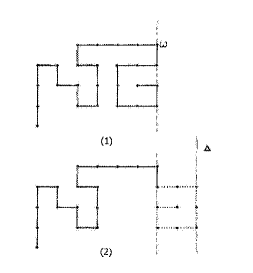
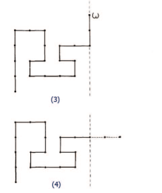
Figure 1.3: A possible move by pivoting, in Sokal’s algorithm (1) Pivot at $\omega$, by reflecting through the dashed line. (2) The resultant conformation showing the reflected part in dotted line. (We can now pivot at $\Delta$)

Figure 1.4: A possible move employing rotation, in Sokal’s algorithm (3) Rotate $90^{o}$ at $\omega$. (4) The result.

Chapter 2 Bond Fluctuation model

Bond fluctuation model is a lattice model for simulating polymer systems. It is useful for obtaining static and dynamic properties of polymers. According to this model, a trial conformation is generated by moving a randomly selected monomer from its current location to a location one lattice spacing away, along one of the possible directions chosen randomly and with equal probability. During the move we must ensure that bond crossing does not occur and self avoidance condition is satisfied. This model retains the advantages of both growth algorithms and Sokal’s algorithm, see below.
Like in a growth algorithm, the move is local i.e.; a trial conformation is generated by moving a randomly selected monomer.
Like in Sokal’s algorithm, we start with a polymer of required size. A trial conformation, generated by local rule, is accepted or rejected by Metropolis algorithm. Thus we generate a Markov chain of lattice polymer conformations; asymptotic part of the chain constitutes a canonical ensemble from which the desired macroscopic properties can be calculated.

2.1 Basic description of the Bond Fluctuation Model (BFM)

On a two dimensional square lattice, each monomer occupies four lattice sites of a unit cell [16, 29]. Each lattice site can at best be part of only one monomer by virtue of self avoidance condition. We implement it on a square lattice with lattice constant unity. Let $l$ denotes length of a bond. Minimum bond length is $l=2$. A bond length less than $2$ violates self avoidance condition. We restrict to bond length less than $4$. This condition ensures that no bond crossing takes place. The possible bond lengths less than $4$ are: $2,\ \sqrt{5},\ \sqrt{8},\ 3,\ \sqrt{10}$ and $\sqrt{13}$. Figure (2.1) shows a bond fluctuating lattice polymer with all possible bond lengths. In the present work, we restrict ourselves to four site model on a two dimension square lattice.

Instead of four site lattice model one can consider one site model i.e., a monomer occupies single lattice site with possible bond lengths between $1$ and $\sqrt{2}$. But in this model there exists certain compact conformations that do not evolve; this renders the model non-ergodic.

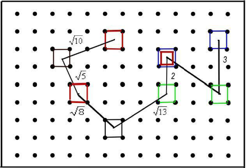
Figure 2.1: A bond fluctuating lattice polymer with all possible bond lengths less than $4$ lattice units is depicted. Monomers shown in same color are non bonded nearest neighbours. Two monomers, not connected by a bond, but separated by a distance $d\ \leq\ \sqrt{13}$ constitute a non-bonded Nearest Neighbour (nbNN) contact.

Figure (2.2) shows trapped conformations with monomers occupying single lattice site. The same conformations with possible moves in case of four site lattice model are also shown in the same figures.

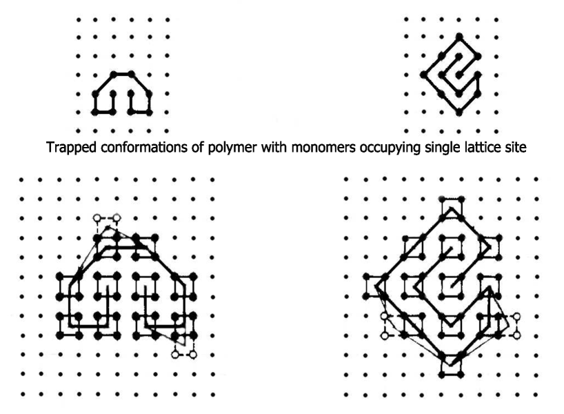
Figure 2.2: Illustration of the problem with ergodicity in one site model. The conformations shown do not evolve. However, the same conformations in four site model evolve and hence ergodic.

We are interested in studying low temperature properties of polymer conformations. Hence we have chosen four site lattice model, which does not suffer from problems arising due to of lack of ergodicity.

2.2 Algorithm

Implementation of Bond Fluctuation model proceeds as follows.

• Step 1: Start with an initial linear self avoiding conformation of a lattice polymer consisting of $N$ monomers.

• $\bf Step\ 2:$ Select a monomer randomly and select one of the four lattice directions randomly with equal probability.

• $\bf Step\ 3:$ Move the selected monomer in the selected direction by one lattice spacing. Call this a trial move.

• $\bf Step\ 4:$ Check if the trial move violates self avoidance condition. If it does, then reject the trial move by placing the monomer in its earlier lattice position and go to step 2.

• $\bf Step\ 5:$ Check if trial move increases the bond length beyond $\sqrt{13}$. If it does, then reject the trial move by placing the monomer in its earlier lattice position and go to step 2.

• $\bf Step\ 6:$ If both requirements self avoidance and bond length restrictions are met then take the trial conformation for further processing through Metropolis or entropic sampling or Wang-Landau algorithms. After processing go to step2.

Figure (2.3) depicts moves that are legal and those that are not legal.

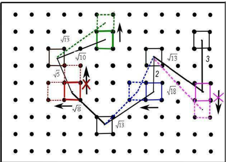
Figure 2.3: Legal moves in Bond Fluctuation Model. These moves do not cut a bond; obeys self avoidance; do not stretch the bond length beyond the set limit. Also shown are moves that are not permitted in the model.

2.3 Dynamics of Bond Fluctuation model

Bond Fluctuation model can be used to find dynamical properties of polymers since this model has the following characteristics.

1. The elementary motion is a random local move.

2. Excluded volume interaction among monomers is modelled through self avoidance condition.

3. During a move there occurs no bond intersection.

4. The algorithm is ergodic .

We have investigated the dynamics of the entire polymer as follows. We start with a self avoiding conformation. We select randomly and with equal probability a monomer and move it by one lattice spacing in such a way that self avoidance condition is met and no bond stretches beyond the prescribed bond length. We carry out this dynamics for a large number of Monte Carlo steps. A Monte Carlo step consists of $N$ moves where $N$ is the number of monomers on the polymer chain. The trace of the centre of mass is depicted in Fig. (2.4), which resembles that of a two dimensional Brownian motion. We have also calculated the mean square deviation of the centre mass and found that it diverges linearly with time. The log-log plot of the mean square deviation is depicted in Fig. (2.5). We get a straight line with slope nearly unity confirming that the centre of mass executes Brownian motion.

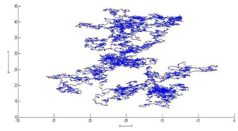
Figure 2.4: Brownian motion of centre of mass of a polymer in two dimension

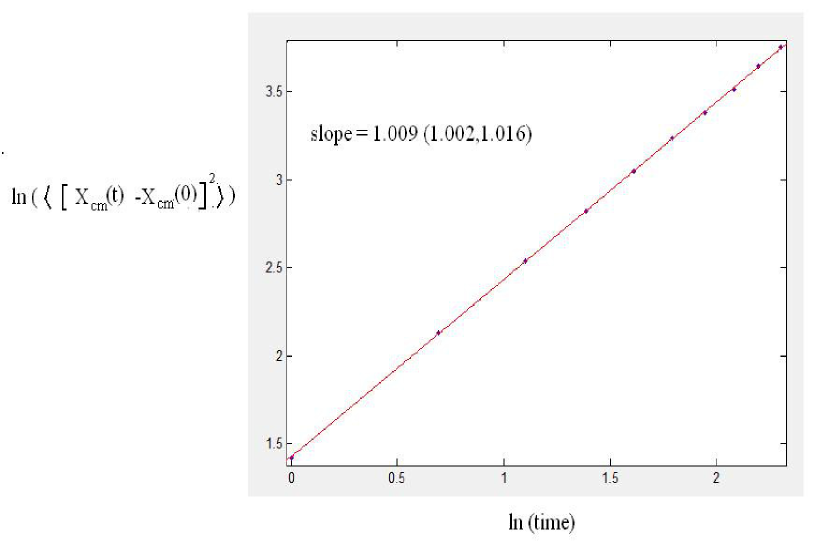
Figure 2.5: Logarithm of mean square deviation of the $x$-coordinate of centre of mass versus logarithm of time

Chapter 3 Monte Carlo Simulation of Bond Fluctuation Model

Bond Fluctuation model on a two dimensional square lattice discussed in the previous chapter can be simulated by employing Metropolis algorithm. The conformations shown in Figs. (3.6, 3.7 and 3.9) are obtained by employing metropolis algorithm on a polymer of length $50$ monomers at low temperature $T=1.2$ and at high temperature $T=2.2$ respectively. A brief description of the Metropolis algorithm is given below

3.1 Metropolis algorithm

In order to calculate equilibrium properties like average energy and average radius of gyration of lattice polymers at a particular temperature, we generate a canonical ensemble by employing Markov chain Monte Carlo methods based on Metropolis algorithm [17]. Metropolis algorithm proceeds as follows.

• Let $C_{i}$ be the current polymer conformation with energy $E_{i}$

• Let $C_{t}$ be the SAW conformation with energy $E_{t}$ generated employing bond fluctuating model.

• If $E_{t}$ $\leq$ $E_{i}$ then accept trial conformation : $C_{i+1}$=$C_{t}$.

• If $E_{t}\ >\ E_{i}$, calculate the ratio of Boltzmann weights
  $p=\exp[-\beta(E_{t}-E_{i})]$. Select a random number $\xi$. If $\xi<p$ accept trial conformation : $C_{i+1}=C_{t}$; else reject the trial conformation and set $C_{i+1}=C_{i}$.

Iterate the whole procedure and generate a Markov chain. The asymptotic part of the Markov chain consists of conformations that belong to a canonical ensemble, at the chosen temperature. The desired macroscopic properties are calculated by taking arithmetic average over the Monte Carlo ensemble.

The conventional Markov chain Monte Carlo methods based on Metropolis algorithm are not suitable for calculating thermal properties like entropy and free energies. We are interested in studying phase transition in a polymer. The nature of the phase transitions is best studied from free energy profiles. To calculate thermal properties we have to go beyond Metropolis algorithm and resort to non-Boltzmann Monte Carlo methods.

The first non-Boltzmann Monte Carlo method called Umbrella Sampling was proposed by Torrie and Valleau [18]. Several variants of Umbrella sampling have since been proposed. They include the multi canonical Monte Carlo method of Berg and Neuhaus [19], entropic sampling of Lee [20], Wang-Landau algorithm [21] and several variants of Wang-Landau algorithm $e.g.$ Frontier sampling [22], JSM technique [23] etc.. For an introduction to Boltzmann and non-Boltzmann Monte Carlo methods, see $e.g.$ [24]. In the present work, we employ Wang Landau algorithm to simulate bond fluctuating lattice polymer. The algorithm is briefly described below.

3.2 Wang-Landau algorithm

In Wang-Landau algorithm we bias the Markov chain to move towards regions of lower entropy. This is carried out as below
Algorithm

• Step1 : Let $g$ denotes the density of states. In lattice polymer problem energy of the polymer equals negative of the number of non-bonded nearest neighbour contacts. The energy is thus an integer. Hence we calculate the density of states at discrete energies. Let $\{g(E_{i})\}$ denote the discrete density of states. Since the density of states is unknown for the system initially, start with $g(E_{k})=1\ \forall\ k$ . Take the Wang-Landau factor $f=2.7183=e$. We start with an arbitrary initial conformation denoted by $C_{0}$ and evolve the chain $C_{0}\to C_{1}\to C_{2}\to\cdots\to C_{i}\to\cdots$ as per Wang-Landau dynamics described below.

• Step 2: Let $C_{i}$ be the current conformation. $\{h(E)\}$ denotes the energy histogram of conformations actually taken by the lattice polymer following Wang-Landau dynamics. At the beginning we set $h(E)=0\ \forall\ E$.

• Step 3: Employing Bond fluctuating model construct a trial conformation $C_{t}$

• step 4: If $g(E(C_{t}))\leq g(E(C_{i}))$ accept trial conformation. Update $h(E(C_{t})=h(E(C_{t})+1$ and $g(E(C_{t}))=g(E(C_{t}))\times f$. Set $C_{i+1}=C_{t}$ and go to step 3

• Step 5: If not, calculate the ratio $\displaystyle{p=\frac{g(E(C_{i}))}{g(E(C_{t}))}}$. Call for a random number $\xi$. If $\xi\leq p$ then accept trial conformation. Update
  $g(E(C_{t}))=g(E(C_{t}))\times f\ {\rm and}\ h(E(C_{t}))=h(E(C_{t}))+1.$ Set $C_{i+1}=C_{t}$ and go to step 3

• Step 6: If $\xi\ >\ p$ reject the trial conformation. Update
  $g(E(C_{i}))=g(E(C_{i})\times f$, $h(E(C_{i}))=h(E(C_{i}))+1$; Set $C_{i+1}=C_{i}$ and go to step3

• Step 7: Sufficiently large number of Monte Carlo sweeps are to be performed to ensure a flat histogram. Check for the flatness of the histogram i.e., all the entries in the histogram should be greater than $\delta\%$ of the average. In all the studies reported in this thesis we have taken $\delta=80$.

• step 8: When the flatness check is passed, $f$ is modified to $\sqrt{f}$ and then go to step 2. This process is continued until $f\sim\exp(10^{-8})$ i.e., $f\approx 1$

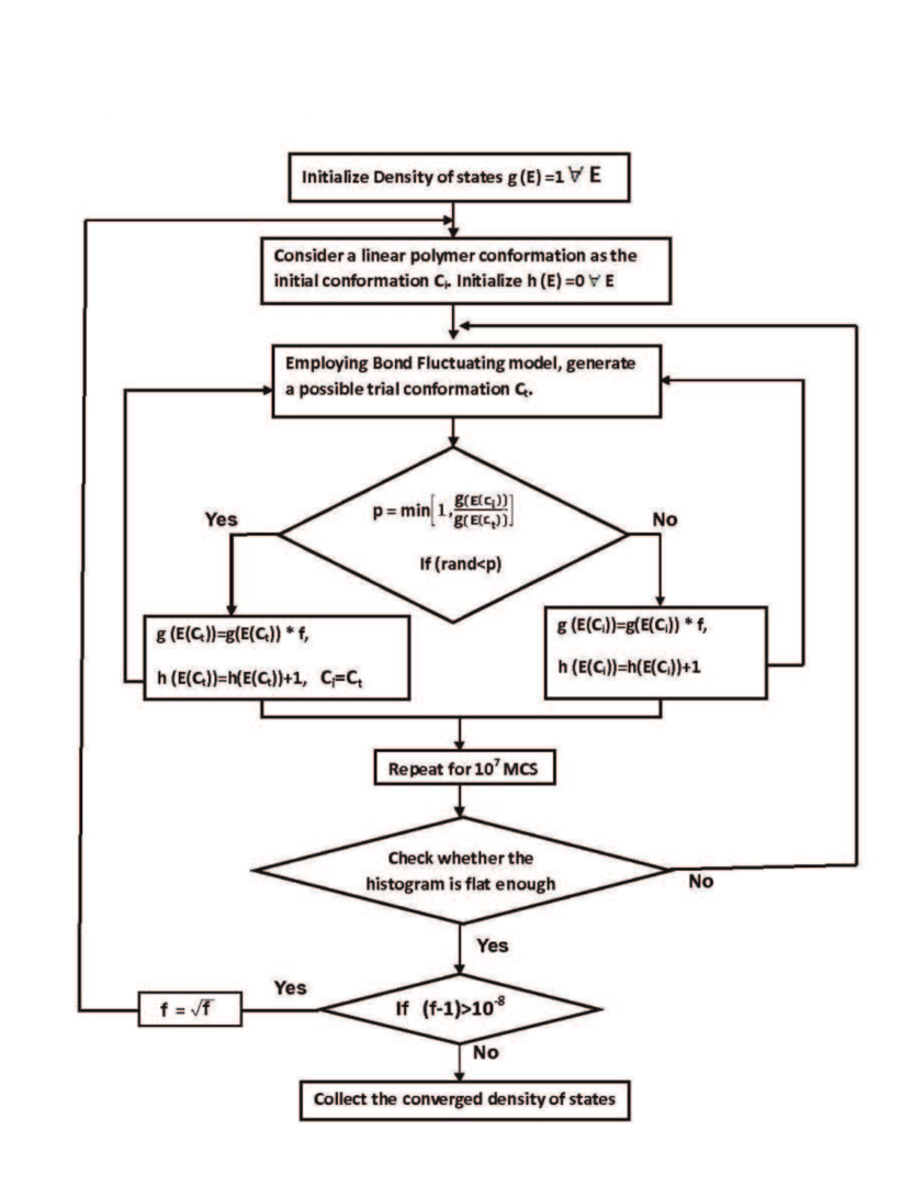
Figure 3.1: Flow chart for the Wang-Landau algorithm

Using the converged density of states, we can calculate micro canonical entropy: $S(E)=k_{B}\ln g(E)$. Employing the standard machinery of thermodynamics, we can calculate all the desired macroscopic properties from the micro canonical entropy function. Helmholtz’s free energy can be calculated as

$$F(T) = -k_{B}T\ln(Z)$$

$$= -k_{B}T\ln\left(\sum_{E}g(E)\exp(-\beta E)\right)$$

$$or$$

$$F(T) = E-TS(E)$$ (3.2)

$$T^{-1} = \frac{\partial S}{\partial E}$$

Internal energy can be calculated as

$$U(T)=\langle E\rangle=\frac{\sum_{E}\ E\ g(E)\ \exp\left[-\beta E\right]}{\sum_{E}\ g(E)\ \exp\left[-\beta E\right]}$$ (3.3)

And the specific heat can be obtained as

$$C_{V}(T)=\frac{\langle E^{2}\rangle-\langle E\rangle^{2}}{k_{B}T^{2}}$$ (3.4)

Alternately we can generate an entropic ensemble of polymer conformations $C_{i}$ employing converged density of states. We can calculate un-weighting-cum-re-weighting factors for each conformation of the entropic ensemble. It is given by

$$W(C_{i})=g(E(C_{i}))\exp[-\beta E(C_{i})]$$ (3.5)

Using this weight we can obtain canonical ensemble average of a macroscopic property say $\eta(C_{i})$ at the desired temperature from the entropic ensemble, see below.

$$\langle\eta(\beta)\rangle=\frac{\sum_{C_{i}}\ \eta(C_{i})W(C_{i})}{\sum_{C_{i}}W(C_{i})}$$ (3.6)

The sum runs over all the conformations of the entropic ensemble.

3.3 Results and Discussions

We have carried out non-Boltzmann Monte Carlo simulation of bond fluctuation model with $N=10,\ 20,\ 30$ and $50$. Figure (3.2) shows the energy histogram for a polymer with $50$ monomers. We consider the energy region : $-130$ to $-20$, where the histogram is reasonably flat, consistent with the $80\%$ flatness criterion described earlier. The micro canonical entropy is given by $S(E)=k_{B}\ln g(E)$. Without loss of generality we set the Boltzmann factor $k_{B}=1$. In this work, all the calculations were carried out by taking $\ln(S(E))$ instead of g(E) to avoid overflow problems. Figure (3.3) shows $\ln(S(E))$ versus $E$.

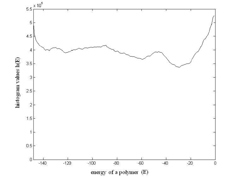
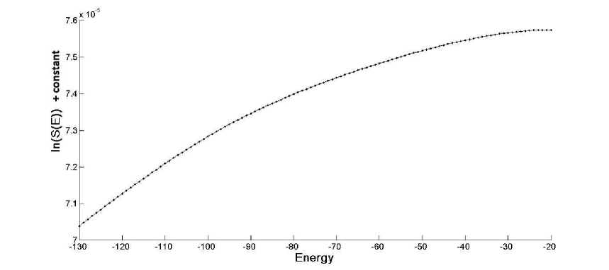
Figure 3.2: Energy histogram, $h(E)$ of lattice polymer of length $50$ monomers. A range of energy from $-130$ to $-20$ is considered; the histogram is reasonably flat in this range.

Figure 3.3: Logarithm of entropy as a function of energy in the range : $-130$ to $-20$. The value of the constant on Y-axis is -16.4124.

3.3.1 Variation of energy with Temperature

As discussed in the first chapter, a compact globule structure is an equilibrium structure at low temperature and an extended coil structure is an equilibrium structure at high temperature. A compact globule structure contains more nbNN contacts compared to extended coil structure. Since $\epsilon=-1$ for an nbNN contact, a compact globule structure has less energy compared to extended coil structure. So the average energy should be less at low temperature and high at high temperature. Figure (3.4) shows average energy calculated from both density of states and from the entropic ensemble (generated in the production run employing un-weighting and re-weighting factors).

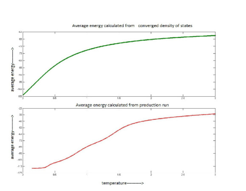
Figure 3.4: Top: Average energy as a function of temperature calculated from the density of states. Bottom: Average energy as a function of temperature calculated over a sample from entropic ensemble. These calculations are done for a polymer of length $50$ monomers

3.3.2 Energy fluctuation

Energy and energy fluctuations are two important macroscopic parameters. Energy fluctuation is defined as $\sigma^{2}_{E}=\langle E^{2}\rangle-\langle E\rangle^{2}$, where the angler brackets denote an average over a canonical ensemble.

Heat capacity is defined as the thermal energy you need to supply to a macroscopic object to raise its temperature by one degree Kelvin. Thus $\displaystyle{C_{V}=\frac{\partial U}{\partial T}}$ where $U$ is the mean internal energy. We have

$$U\equiv\langle E\rangle=\frac{\sum_{r}E_{r}\exp\left[-\beta E_{r}\right]}{\sum_{r}\exp\left[-\beta E_{r}\right]}$$ (3.7)

In the above the sum over $r$ denotes a sum over all the microstates of the closed system.

If we take the partial derivative of $U$ with respect to $\beta$, we get,

$$\frac{\partial U}{\partial\beta}=-\langle E^{2}\rangle+\langle E\rangle^{2}$$ (3.8)

It follows then

$$\langle(\Delta E)^{2}\rangle\equiv\langle E^{2}\rangle-\langle E\rangle^{2}=-\left(\frac{\partial U}{\partial\beta}\right)=k_{B}T^{2}\left(\frac{\partial U}{\partial T}\right)=k_{B}T^{2}C_{V}.$$ (3.9)

$$C_{V}=\frac{1}{k_{B}T^{2}}(\langle E^{2}\rangle-\langle E\rangle^{2})$$ (3.10)

At transition temperature specific heat profile has a peak showing the signature of the phase transition .

The results on heat capacity ($C_{V}$) as a function of temperature are depicted in Fig. (3.5), for $N=10,\ 20,\ 30$ and $50$. As the system size increases the heat capacity curves peak more and more sharply. In the Fig. (3.5) we see a sharp peak at $T=T_{C1}=0.83$ and a broad peak at $T=T_{C2}=1.6\ >\ T_{C1}$. The temperature at which $C_{V}$ is maximum gives an estimate of the transition temperature $T_{C}$.

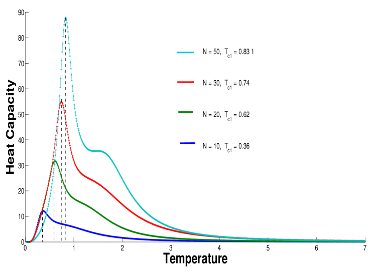
Figure 3.5: Heat capacity as a function of temperature for polymers of length $N\ =\ 10,\ 20,\ 30$ and $50$ monomers. For $N=50$, the sharp peak at $T=T_{C1}=0.83$ corresponds to crystallization transition and the broad peak at $T_{C2}=1.6$ corresponds to coil-globule transition.

The broader peak corresponds to a phase transition from extended coil to compact globule structure. For a self attracting chain, this transition is caused by the competition between excluded volume repulsion and attraction due to segment-segment interaction and configurational entropy. Transition temperature, $T_{C2}$ is found to be $1.6$. Figures (3.6 and 3.7) show configurations of a polymer of length $50$ monomers at temperatures $1.2$, below $T_{C2}$ and at $2.2$, above $T_{C2}$ respectively. Figure (3.6) shows a compact globule structure of a polymer of length $50$ monomers whose radius of gyration is $7.6026$ at at $T=1.2$. Figure (3.7) shows an extended coil structure of a polymer of length $50$ monomers whose radius of gyration is $14.3639$ at $T=2.2$. These conformations are obtained by simulating bond fluctuation model of isolated polymer of length $50$ monomers employing Metropolis algorithm.

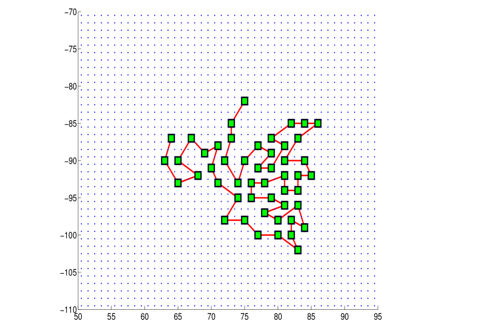
Figure 3.6: Compact globule conformation at $T_{C1}\ <T=1.2\ <\ T_{C2}$. The radius of gyration for this conformation is $7.6026$.

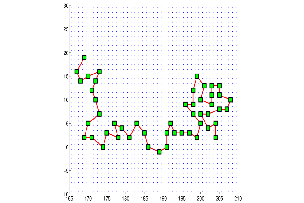
Figure 3.7: Extended coil conformation at $T=2.2\ >\ T_{C2}$. The radius of gyration for this conformation is $14.3639$.

Figure (3.8) shows heat capacity profile of a polymer of lengths $10,\ 30$ and $50$ monomers. The heat capacity profiles have each a peak signalling coil-globule phase transition. The peaks become sharper as $N$ increases. The calculations were done considering only a narrow energy region around the broad peak depicted in Fig. (3.5). The transition temperature for a polymer of length $50$ monomers is found to be $1.96$.

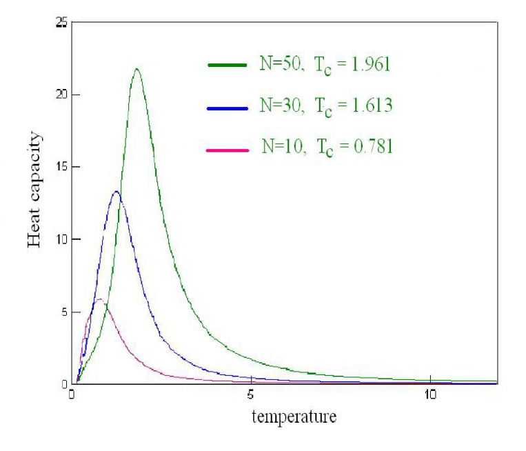
Figure 3.8: Heat capacity curve for polymers of length $10,\ 30,\ and\ 50$ monomers when a narrow energy region around the broad peak in Fig. (3.4) is considered. We see a sharp peak at $T_{C2}=1.96$ corresponding to coil-globule transition, for $N=50$.

The sharp peak in the heat capacity profile seen at a lower temperature in Fig. (3.5), depicts a phase transition which could be the crystallization as discussed in [25] or the solid-liquid transition as described in [26].

Figure (3.9) shows an extremely compact structure of a polymer of length $50$ monomers at a $T=0.4$ whose radius of gyration is $5.8$. The radius of gyration of this conformation is found to be less when compared to globular structure at $T=1.2$ whose radius of gyration is $7.6$.

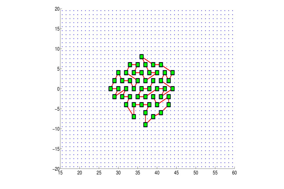
Figure 3.9: Extremely compact conformation at $T=0.4\ <\ T_{C1}$. The radius of gyration for this conformation is $5.7659$.

Chapter 4 Free Energy and Landau Free Energy

4.1 Introduction

In this chapter we shall provide a brief introduction to Helmholtz free energy or simply free energy for an equilibrium system. We shall describe free energy for a closed system (canonical ensemble) and for an isolated system (microcanonical ensemble). Besides we shall consider the phenomenological free energy introduced by Landau for the bond fluctuating lattice polymer.

4.1.1 Free energy for a closed system

For a closed system, free energy is function of temperature and other thermodynamic variables like volume, $V$ and number of molecules, $N$. It is written as

$$F(T,V,N)=U(S,V,N)-TS$$ (4.1)

In the Right Hand Side (RHS) we eliminate $S$ by expressing it as a function $T$, $V$ and $N$, see below.

$$T(S,V,N)=\left(\frac{\partial U}{\partial S}\right)_{V,N}.$$ (4.2)

In statistical Mechanics, free energy for a closed system is related to canonical partition function, Q(T,V,N), as shown below.

$$F(T,V,N) = -k_{B}T\ln Q(T,V,N)$$ (4.3)

$$Q(T,V,N) = \sum_{C}\exp\left(-\frac{E(C)}{k_{B}T}\right),$$ (4.4)

Energy of the closed system is given by

$$U(T,V,N)=\langle E\rangle=\frac{1}{Q(T,V,N)}\sum_{C}E(C)\exp(-\beta E(C))$$ (4.5)

where the sum runs over all microstates of the closed system.

4.1.2 Free energy for an isolated system

For an isolated system, microcanonical free energy is a function of energy. We start with $S\equiv S(U,V,N)$. Wang Landau algorithm gives us an estimate of entropy up to an additive constant. Microcanonical Free energy is then given by

$$F(U,V,N) = U-T(U,V,N)S(U,V,N)$$ (4.6)

$$\left(\frac{\partial S}{\partial U}\right)_{V,N} = \frac{1}{T(U,V,N)}$$ (4.7)

4.2 Landau Free energy

Free energy is either a function of energy (for an isolated equilibrium system) or a function of Temperature (for a closed system). For any equilibrium system, isolated or closed, $F$ cannot be simultaneously a function of both energy and temperature. This is because,

• An isolated system with fixed energy has a unique temperature.

• A closed system at a given temperature has unique energy.

Suppose we want to estimate free energy for an energy different from the equilibrium energy $U$. Let us denote such a free energy by the symbol $F_{L}$, see below. Clearly,

$$F_{L}(E,T,V)\geq F(E=U,T,V),$$ (4.8)

since equilibrium is characterized by minimum free energy. Notice that in the above equation we have written $F_{L}$ as a function of both $E$ and $T$. This is legitimate since we are inquiring about a system not in equilibrium. The right hand side of the above equation is equilibrium free energy:
$F_{L}(E=U,T,V)=F(T,V)$. The difference

$$\delta F=F_{L}(E\neq U,T,V)-F(E=U,T,V)$$ (4.9)

can be thought of as a penalty we have to incur if we want to keep the system in a state with energy $E\neq U$. This corresponds to the phenomenological Landau free energy , and hence the notation $F_{L}$; see [27] for a description of Landau/Landau-Ginzburg free energy.

In Eq. (4.8) equality obtains when $E=\langle E\rangle=U(T)$, and $\langle E\rangle$ denotes an average over a canonical ensemble, at temperature $T$.

Landau free energy can be calculated as follows. In thermodynamics, start with $S\equiv~{}S(U)$ and calculate $F_{L}(U,T)=U-TS(U)$, assuming $U$ and $T$ to be independent of each other.

In statistical mechanics we define $F(T)$ as

$$F(T)=-k_{B}T\ln\sum_{C}\exp[-\beta E(C)],$$ (4.10)

where the sum is taken over all microstates of the closed system. However for a given temperature $T$, the contribution to the partition sum comes predominantly from those conformations having energy $E=\langle E\rangle=U(T)$. Hence we can express free energy as

$$F(T)=-k_{B}T\ln\sum_{C}\delta(E(C)-U(T))\exp[-\beta E(C)]$$ (4.14)

In the above if we replace U(T) by E, we get Landau free energy,

$$F_{L}(E,T)=-k_{B}T\ln\sum_{C}\delta(E(C)-E)\exp[-\beta E(C)]$$ (4.15)

Note that in the above, the presence of Dirac delta function ensures that the sum runs only over those microstates for which $E(C)=E$.

4.2.1 Free energy calculations

Employing Wang Landau algorithm to simulate bond fluctuation model, we have obtained converged density of states, $g(E_{i})$. We consider all possible discrete energies $E_{i}$ of the lattice polymer. Microcanonical entropy is given by $S(E_{i})=k_{B}\ln g(E_{i})$. Without loss of generality we take $k_{B}$=1. Landau Free energy $F_{L}(E_{i},T)$ can be calculated using any one of the following two equations

$$F_{L}(E_{i},T) = E_{i}-TS(E_{i})$$ (4.16)

$$F_{L}(E_{i},T) = -k_{B}T\ln\left[g(E_{i})\exp(-\beta E_{i})\right]$$ (4.17)

We have used both the above expressions and found that they give the same results. We have calculated Landau free energy for lattice polymers with $10,\ 20,\ 30,\ 40$ and $50$ monomers. The results are presented and discussed below.

4.3 Results and Discussions

From the heat capacity curve for a polymer of length $50$ we found that there are two transitions. One corresponding to transition from extended coil phase to compact globule phase at a temperature $T=1.6$. The other corresponds to crystallization transition at temperature of $T=0.83$.

We have checked Landau free energy profile, $F_{L}(T,E)$ versus $E$, for a polymer of length $50$ monomers for different temperatures. We found that a coil-globule transition occurs at a temperature of $T_{C2}=1.71$. Figures (4.1, 4.2, and 4.3) correspond to Landau free energy versus energy for three values of temperature, one below, one at, and one above the transition temperature of $1.71$.

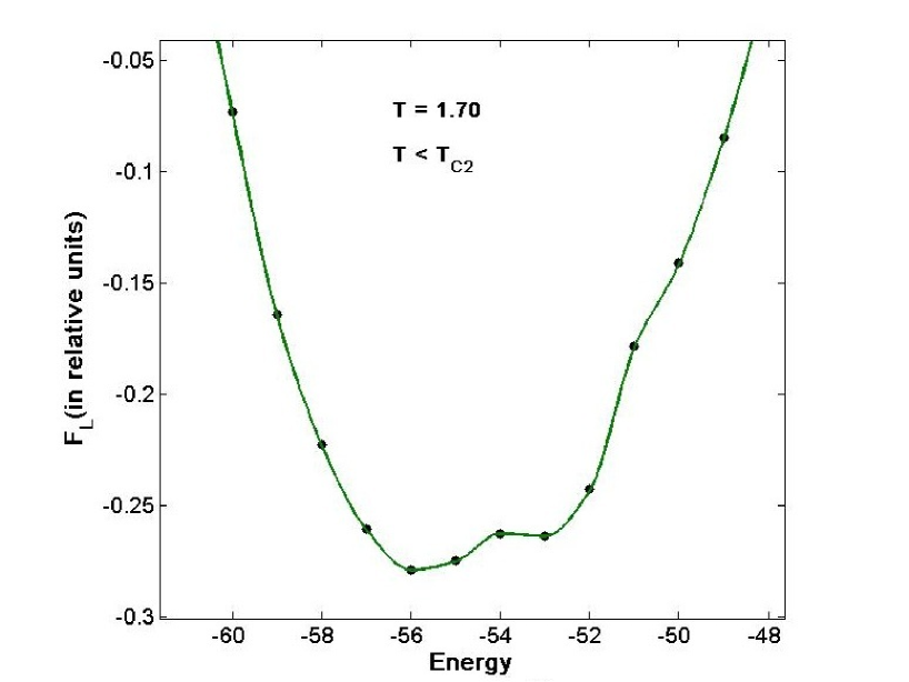
Figure 4.1: Free energy versus energy for $T=1.70\ <\ T_{C2}$ for an isolated polymer of length $50$ monomers. A globule structure with low energy is the stable state and an extended coil structure with high energy is the meta stable state. The values shown on the y-axis are $F_{L}+constant$ (constant=59174).

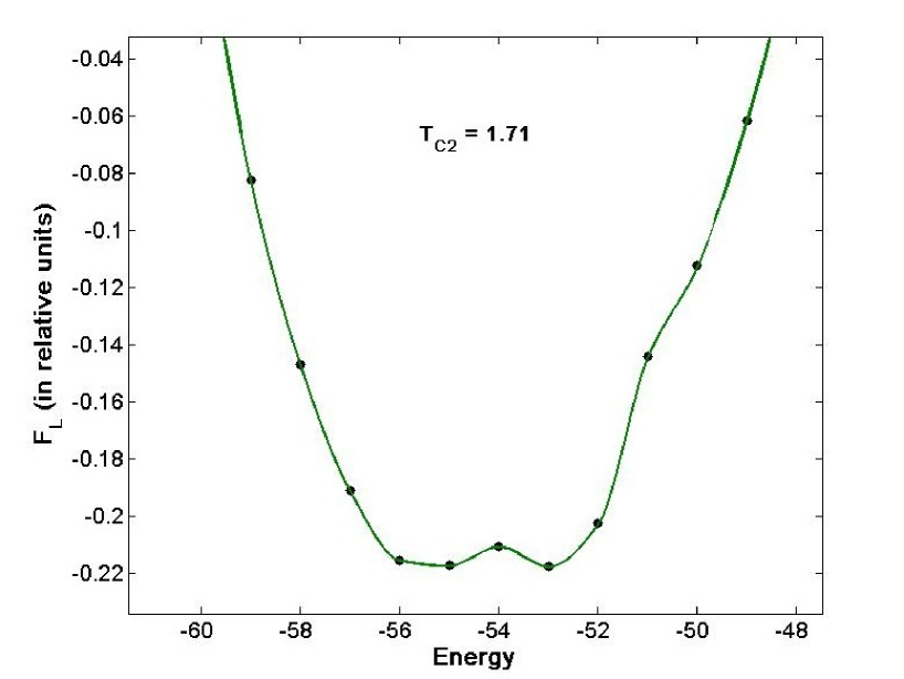
Figure 4.2: Free energy versus energy for $T=T_{C2}=1.71$ for an isolated polymer of length $50$ monomers. Both compact-globule and extended-coil phases are stable. The values shown on the Yaxis are $F_{L}+constant$ (constant=60066).

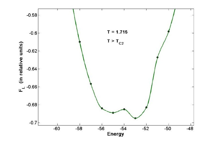
Figure 4.3: Free energy versus energy for $T=1.715\ >\ T_{C2}$ for an isolated polymer of length $50$ monomers. An extended-coil phase with high energy is stable; a compact-globule phase with low energy is the meta stable. The values shown on the Yaxis are $F_{L}+constant$ (constant=60241).

From these figures we see that for $T\ <\ T_{C2}$, there is stable minimum that corresponds to collapsed phase and and a meta-stable minimum that corresponds to extended coil phase. At $T=T_{C}$ both these phases co-exist. For $T\ >\ T_{C2}$ the extended coil phase is stable and the collapsed globule phase is meta stable. The phase transition is first order. We find that the free energy barriers are small; this is due to the fact that the lattice polymers simulated are not long.

We have calculated Landau free energy profile for the transition that corresponds to the peak in the specific heat curve at $T=T_{C1}<T_{C2}$. From Fig. (3.4) we find that $T_{C1}=0.83$ for a polymer of size $50$. From Landau free energy curve the transition temperature is found to be $0.8$. Figures (4.4, 4.5, 4.6) show Landau free energy $\it versus$ energy for three values of temperature, one below, one at and one above the transition temperature, $T_{C1}=0.8$. Landau free energy curve exhibits two minima at all temperatures close to $T_{C1}$. At $T\ <\ T_{C1}$ the polymer conformations are extremely compact. This phase is usually referred to as crystalline phase, see [25]. We find that this transition is also discontinuous.

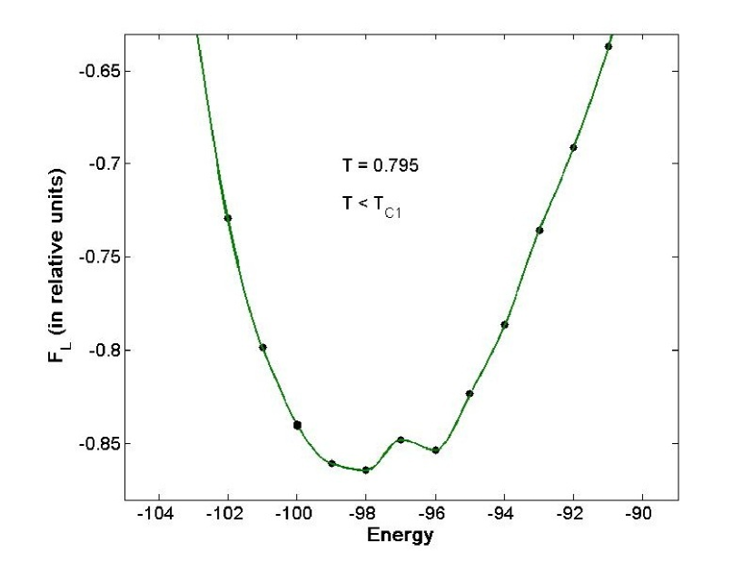
Figure 4.4: Free energy versus energy for $T=0.795\ <\ T_{C1}$ for an isolated polymer of length $50$ monomers. Crystalline structure at low energy is the stable; a globule structure with high energy is meta stable state. The values shown on Y-axis are $F_{L}+constant$ (constant=27965).

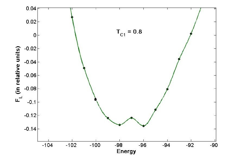
Figure 4.5: Free energy versus energy for $T=T_{C1}=0.8$ for an isolated polymer of length $50$ monomers. Both crystalline and globule phases coexist. The values shown on Y-axis are $F_{L}+constant$ (constant=28141).

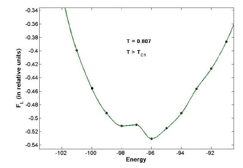
Figure 4.6: Free energy versus energy for $T=0.807\ >\ T_{C1}$ for an isolated polymer of length $50$ monomers. Globule phase with high energy is stable and crystalline phase with low energy is meta stable. The values shown on Y-axis are $F_{L}+constant$ (constant=28386).

The character of the phase transition can also be analysed using the fourth order Binder’s cumulant, $V_{L}(T)$ [28], defined as follows.

$$V_{L}(T)=1-\frac{\langle E^{4}\rangle_{L}}{3\langle E^{2}\rangle^{2}_{L}}$$ (4.18)

where $E$ is the energy. Binder’s reduced cumulant, $V_{L}(T)$ are shown in Fig. (4.7) for polymers of length $10,\ 20,\ 30$ and $50$. We observe that the curves are typical of discontinuous phase transition.

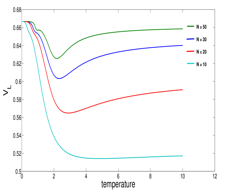
Figure 4.7: Binder’s reduced cumulant versus temperature for an isolated polymer. The transition is first order.

Chapter 5 Polymer in the presence of attractive walls

5.1 Polymer near an attractive wall

Polymer near an impenetrable attractive wall finds applications in adhesion, lubrication, colloid stabilization, chromatography, microelectronic devices, biomedical problems etc.[30]. Since the wall is attractive, the conformations that make contact with the wall have lower energy as compared to those away and not making any contact with the wall. However entropy would be smaller for polymers that make contact with the wall. These competing processes would result in adsorption-desorption transition. If, simultaneously, there is also segment-segment attraction in the polymer, there is a possibility of a collapse transition both in the desorbed and in the adsorbed states [31]. Since the wall is attractive, it contributes an energy $\epsilon_{s}=-1$ for each contact the polymer makes with the wall.

A contact with the wall lowers the energy of the polymer. However it also leads to decrease in entropy. Entropy increases rather steeply with increase of energy. At any given temperature what kind of conformation a polymer takes is completely determined by the competition between energy and entropy. At low temperatures a polymer prefers to get adsorbed on the surface since it leads to lower energy. At high temperatures the polymer would prefer to move away from the wall since that facilitates increase of entropy. Hence desorbed behaviour would prevail at higher temperature.

We model the wall as a long straight polymer fixed parallel to y-axis. This fixed polymer has fixed bond length of $2$. Each monomer of the wall occupies four lattice sites see Figs. (5.2,  5.3). Let $\epsilon_{s}$ denote the energy associated with a contact between a monomer of the polymer and that of the wall. Let $N_{s}$ be the number of contacts between the polymer and the wall. Let $N_{u}$ denote the number of nbNN contacts in the polymer. Total energy of the polymer is thus given by $E=N_{s}\epsilon_{s}+N_{u}\epsilon$.

In our work we have set $\epsilon_{s}=\epsilon=-1$. In other words the segment-segment interaction and polymer-wall interaction are both treated in identical fashion . We employ Wang-Landau algorithm, as described chapter (3), to simulate an entropic ensemble of polymer conformations. We have also employed Metropolis algorithm to generate typical equilibrium conformations at the desired temperatures.

We have obtained converged density of states for polymer near an attractive wall. All the standard machineries we had employed and described in the third and fourth chapters are again used here to calculate heat capacity, Landau free energy and Binder’s cumulant.

The heat capacity curves for polymer of length $N=40$ and $50$ are shown in the Fig. (5.1). The sharp peak corresponds to transition from adsorbed collapsed state to adsorbed extended state and the transition temperature is $T_{C}=0.88$ . We conjecture that the broad shoulder corresponds to adsorption-desorption transition. However we are not able to characterize this transition in terms of free energy profiles or Binder’s cumulant. May be we should simulate longer polymers to get calculate these quantities.

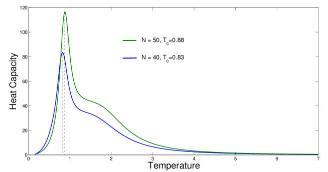
Figure 5.1: Heat capacity curves for polymers of length $40$ and $50$ monomers in the presence of an attractive wall. The sharp peak at $T_{C}$=0.88 corresponds to transition from adsorbed-extended phase to adsorbed-collapsed phase.

At low temperature $(T=0.7\ <\ T_{C})$, a part of the polymer gets stuck to the wall and the dangling part forms a layer over it. This results in a compact structure adsorbed to the wall with lower energy. At high temperature
$(T=1.3\ >\ T_{C})$, the polymer tries to increase its entropy by extending itself over the wall. At very high temperatures $(T>2.6)$ the polymer gets detached from the wall and behaves like an isolated polymer. Figures (5.2 and 5.3) show conformations of a polymer of length $50$ monomers at a low temperature $T=0.7$ and at high temperature $T=1.3$ respectively. Figure (5.4) shows polymer far away from the wall at very high temperature $T=2.8$.

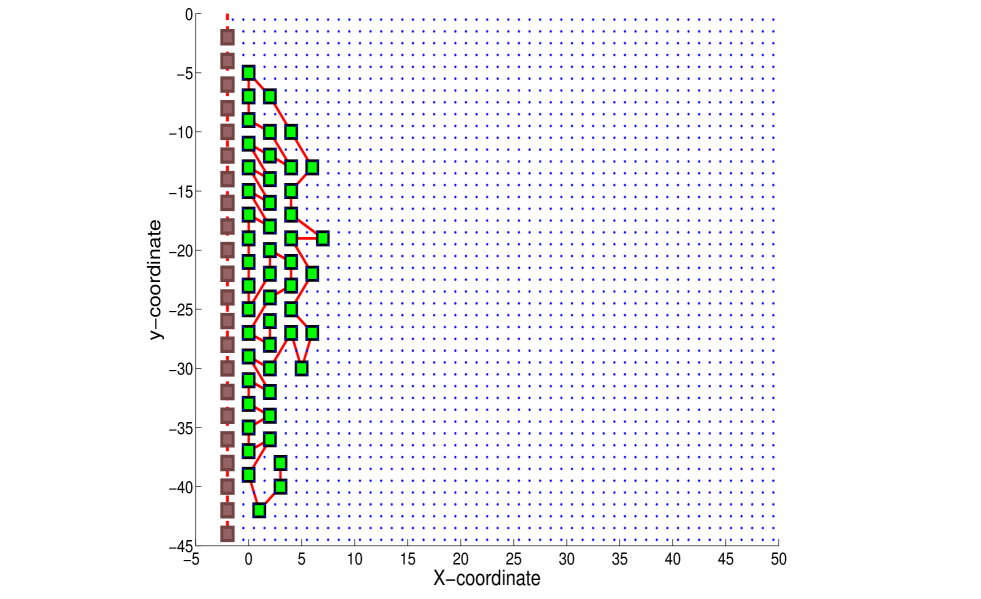
Figure 5.2: Compact conformation of a polymer of length $50$ monomers in the presence of an attractive wall at $T=0.7\ <\ T_{C}$; the radius of gyration of this conformation is $9.7666$. This figure shows a segment of the polymer adsorbed to the wall; the remaining segment forms a layer over the adsorbed part.

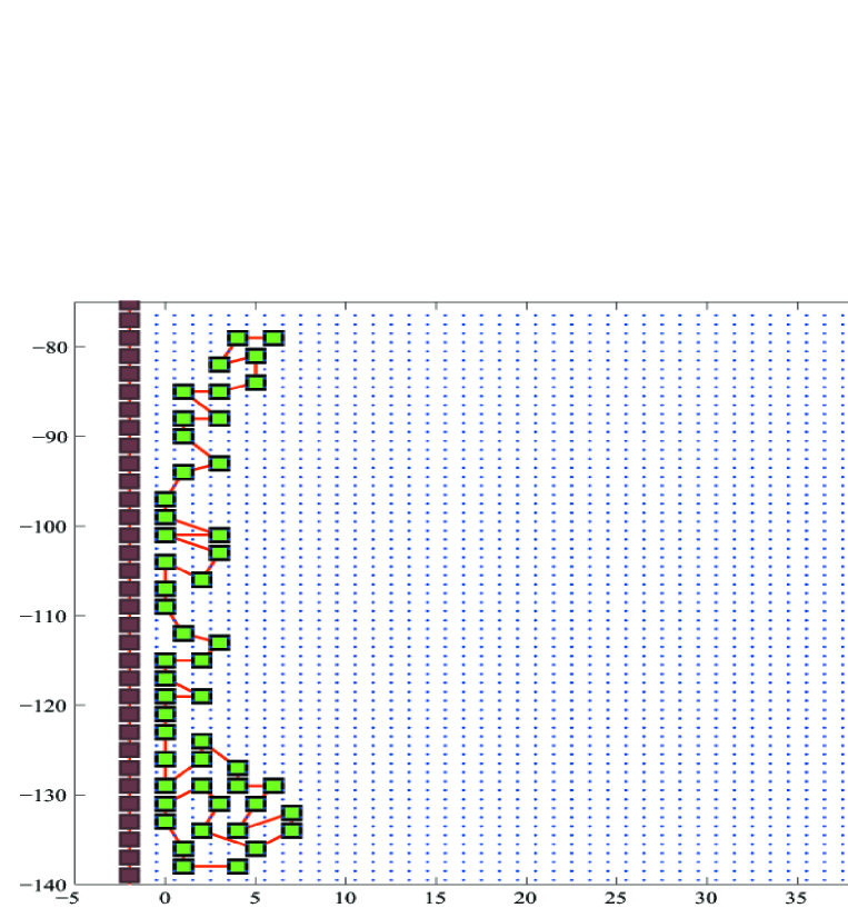
Figure 5.3: Extended conformation of polymer of length $50$ monomers in the presence of an attractive wall at $T=1.3\ >\ T_{C}$; the radius of gyration of this conformation is $18.8566$. This figure shows conformation extended over the wall.

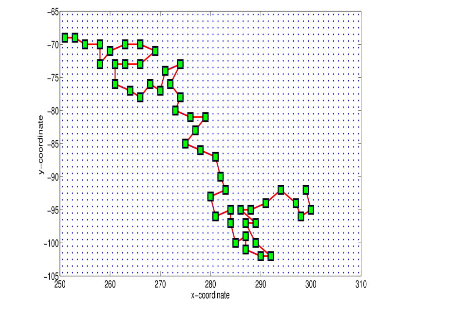
Figure 5.4: Conformation of polymer of length $50$ monomers detached from an attractive wall at $T=2.8$; the radius of gyration of this conformation is $16.9655$
The conformations shown here are obtained by simulating bond fluctuation model of a polymer of length $50$ monomers near an attractive wall employing Metropolis algorithm.

By analysing a narrow energy region where the coil globule transition occurs, we have obtained specific heat curves for polymer of length $10,\ 20,\ 30$ and $50$ monomers in the presence of the wall. These are shown in Figs. (5.5 - 5.8). For comparison we have reproduced the specific heat profiles for a free polymer. From the figures, $T_{C}$ for a polymer near wall is found to be less than $T_{C}$ for isolated polymer. This difference is larger for longer polymers.

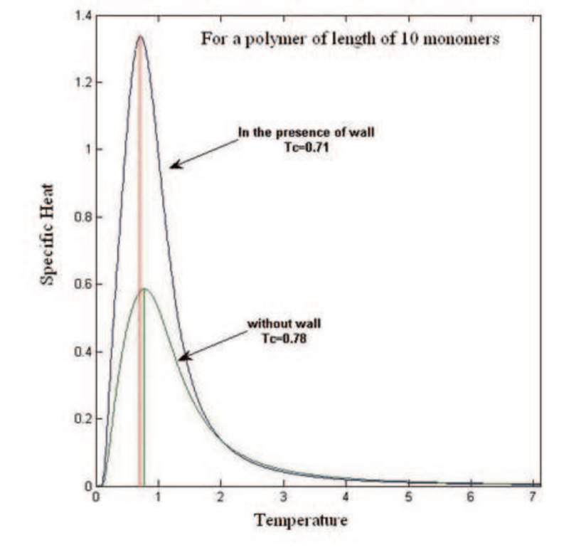
Figure 5.5: Specific heat curves for a polymer of length $10$ monomers with and without wall.

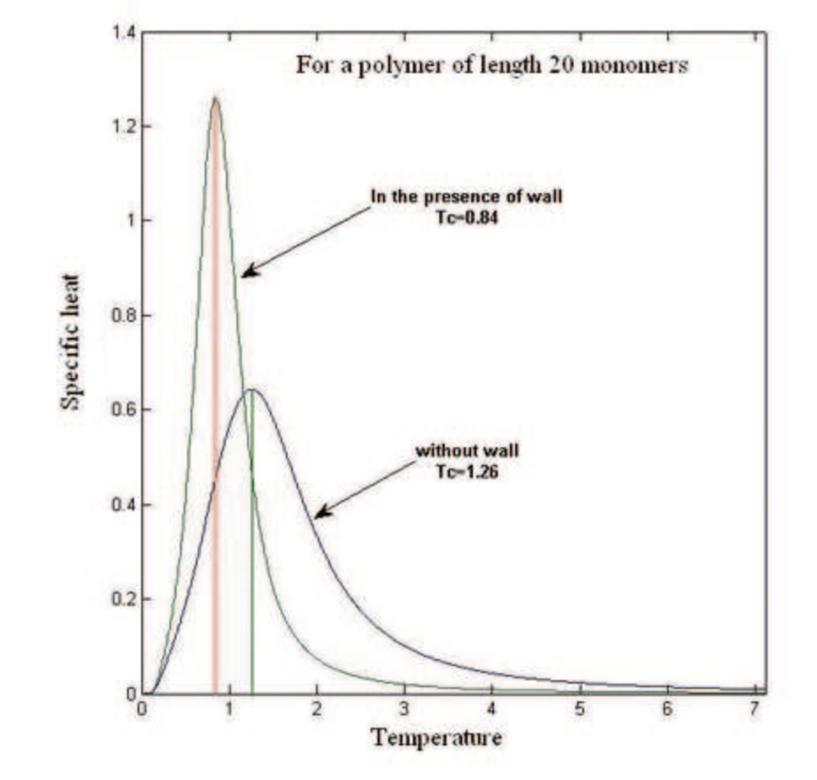
Figure 5.6: Specific heat curves for a polymer of length $20$ monomers with and without wall.

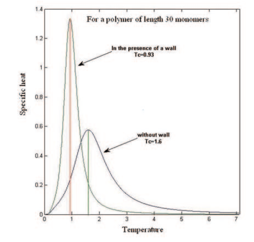
Figure 5.7: Specific heat curves for a polymer of length $30$ monomers with and without wall.

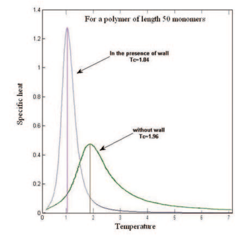
Figure 5.8: Specific heat curves for a polymer of length $50$ monomers with and without wall.

From specific heat curve of a polymer of length $50$ in the presence of a wall the transition temperature is found to be $1.04$. We have obtained Landau free energy profile for transition from adsorbed-collapsed state to adsorbed-extended state. These are shown in Figs. (5.9, 5.10 and 5.11). From Landau free energy profile, critical temperature is found to be $0.91$. The transition from adsorbed-extended to adsorbed-collapsed phase is found to be first order. Figure (5.12) shows Binder’s fourth cumulant curves which again confirms that the transition is first order.

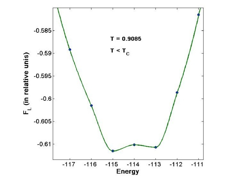
Figure 5.9: Free energy versus energy at $T=0.9085\ <\ T_{C}$ for a polymer of length $50$ monomers near wall. he values shown on Y-axis are $F_{L}+constant$ (constant=45611864).

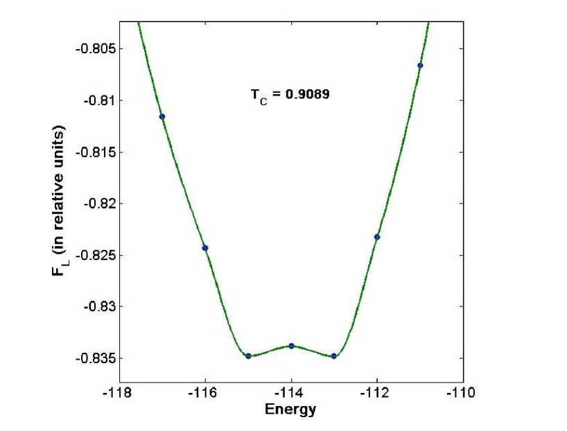
Figure 5.10: Free energy versus energy at $T=T_{C}=0.9089$ for a polymer of length $50$ monomers near wall. The values shown on Y-axis are $F_{L}+constant$ (constant=45631946).

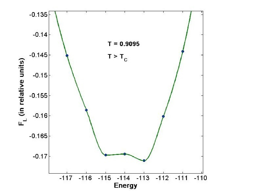
Figure 5.11: Free energy $\it versus$ energy above $T=0.9095\ >\ T_{C}$ for a polymer of length $50$ monomers near wall. The values shown on Y-axis are $F_{L}+constant$ (constant=45662070).

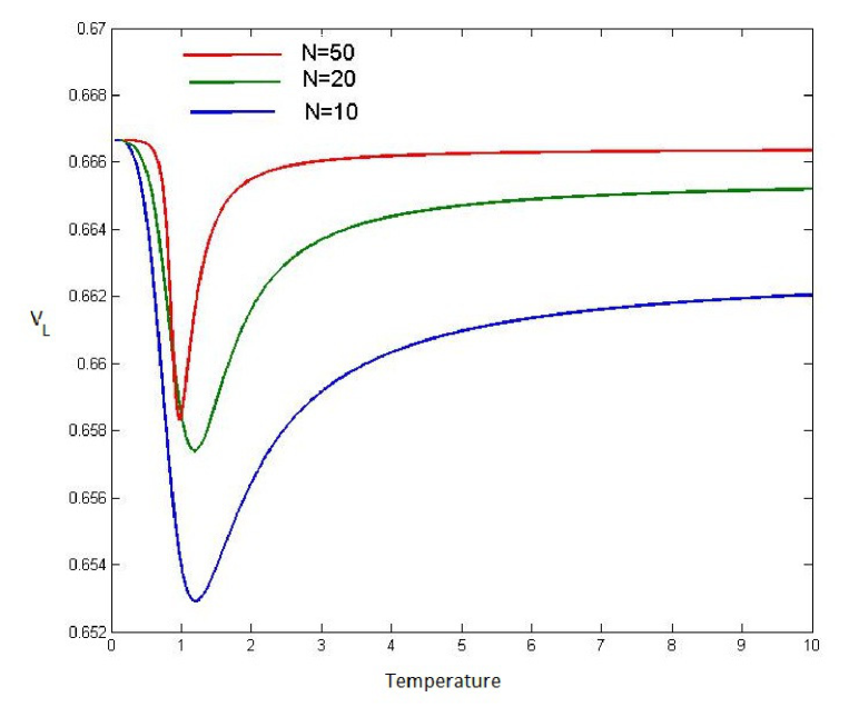
Figure 5.12: Binder’s cumulant versus temperature for a polymer near an attractive wall. The transition is discontinuous.

5.2 Polymer confined between two attractive walls

In this section we study coil to globule transition of a polymer confined between two attractive parallel impenetrable walls in two dimensional lattice [32]. We model the walls in the same way as we did in case of single wall. The interaction with walls is taken as the same as monomer-monomer interactions. The phase transition not only depends on the monomer-monomer interaction and polymer - wall interaction but also on the distance between the walls. If the walls are far separated they will have no effect on the polymer. Hence in this work we have taken the separation distance as $12$ lattice units and simulated polymers of lengths $N=10,\ 20,\ 30$ and $40$ monomers.

Employing bond fluctuation model and Wang-Landau algorithm we get converged density of states of a polymer confined between two walls.

Heat capacity curve shown in Fig. (5.13) gives the coil globule transition temperature as $0.89$ for a polymer of size $40$ monomers. Figure (5.14) shows a compact conformation of the polymer of length $40$ monomers confined between the walls separated by a distance of $12$ lattice units at low temperature of $T=0.74\ <\ T_{C})$; the radius of gyration of the polymer conformation shown in the figure is $6.0413$. Figure (5.15) shows extended conformation of the same polymer at high temperature of $T=1.6\ >\ T_{C})$; the radius of gyration of this conformation is $9.9539$. These conformations have been obtained employing Metropolis algorithm.

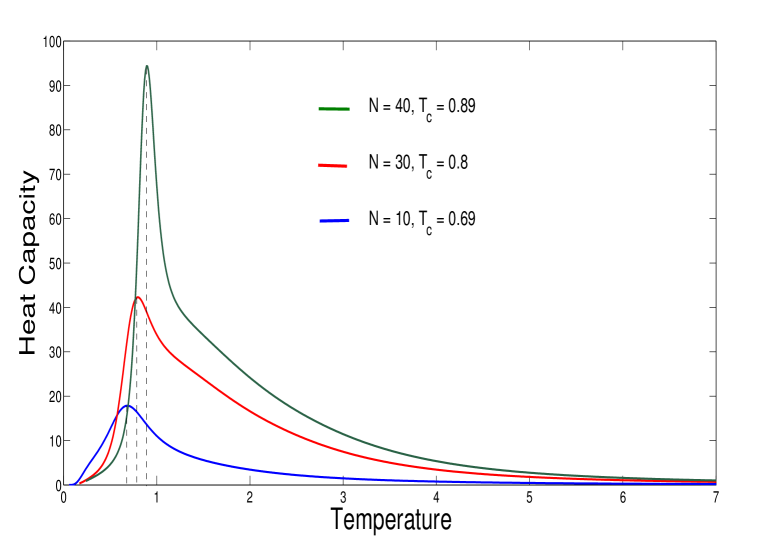
Figure 5.13: Heat capacity profile for polymers of length $10,\ 30\ and\ 40$ monomers confined between two walls separated by distance of $12$ units. Sharp peak at $T_{C}=0.89$, for a polymer of length $40$ monomers, indicates coil-globule transition.

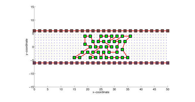
Figure 5.14: Compact conformation of a polymer of length $40$ monomers confined between two walls separated by distance of $12$ units at $T=0.74\ <\ T_{C}$. The radius of gyration for this conformation is $6.0413$. This conformation belongs to a canonical ensemble simulated employing Metropolis algorithm.

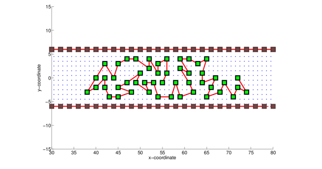
Figure 5.15: Extended conformation of polymer of length $40$ monomers confined between two walls separated by distance of $12$ lattice units at $T=1.6\ >\ T_{C}$; the radius of gyration for this conformation is $9.9539$. This conformation belongs to a canonical ensemble simulated employing Metropolis algorithm.

We have obtained Landau free energy profile for transition from extended phase to collapsed phase for a confined polymer of length $40$. These are shown in Figs. (5.16, 5.17 and 5.18). From Landau free energy profile, critical temperature is found to be $0.89$. The transition is first order. Figure (5.19) shows Binder’s fourth cumulant which confirms that the transition is discontinuous.

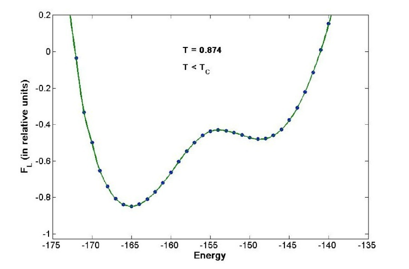
Figure 5.16: Landau free energy versus energy for a polymer of length $40$ monomers confined between walls separated by $12$ lattice units; the temperature is $T=0.874\ <\ T_{C})$. The values shown on Y-axis are $F_{L}+constant$ (constant=49378985).

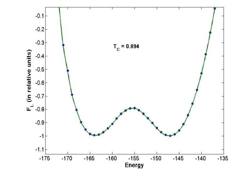
Figure 5.17: Landau free energy versus energy for a polymer of length $40$ monomers confined between walls separated by $12$ lattice units; the temperature is $T=T_{C}=0.891$. The values shown on Yaxis are $F_{L}+constant$ (constant=50508935).

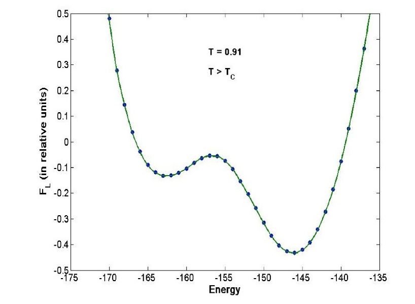
Figure 5.18: Landau free energy versus energy for a polymer of length $40$ monomers confined between walls separated by $12$ lattice units; the temperature is $T=0.91\ >\ T_{C}$. The values shown on Y-axis are $F_{L}+constant$ (constant=51412896).

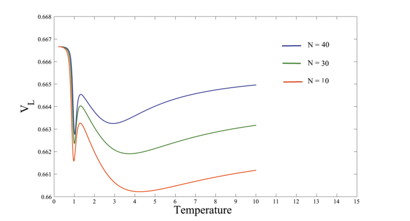
Figure 5.19: Binder’s fourth cumulant versus temperature for polymer confined in double wall; the transition is first order.

Chapter 6 Conclusions

In this report we have investigated the phase behaviour of a linear homopolymer. We have considered attractive interaction between segments of the polymer. We have also investigated the polymer in the presence of a single attracting wall and two walls that confine the polymer.

We have employed the Bond Fluctuation model on a two dimensional square lattice. Each monomer occupies four lattice sites. Self avoidance implies that a lattice site can at best belong to one monomer. The bond length can fluctuate between $2$ and $4$ lattice units.

We have employed Wang Landau algorithm for characterizing the phase transition in the bond fluctuating lattice polymer. Wang-Landau algorithm simulates an entropic ensemble, which is unphysical. Un-weighting and re-weighting of the conformations of the entropic ensemble are required for extracting physical canonical ensemble averages at desired temperatures. The converged density of states which is responsible for flattening of the energy histogram can be directly used for estimating microcanonical and canonical entropies and free energies besides phenomenological Landau free energy and Binder’s cumulant. We have also employed conventional Markov chain Monte Carlo simulation employing Metropolis algorithm to depict typical conformations belonging to canonical ensemble at the desired temperatures. We have simulated polymers with number of monomers ranging from $10$ to $50$.

The principle conclusions of our study are listed below:

• For a free standing polymer we find there are two transitions. The one at a higher temperature corresponds to collapse transition. The one at a lower temperature is crystallization transition. From Landau free energy profiles and Binder’s cumulant we find that both the transitions are discontinuous.

• When a wall is present, we find indications of two transitions, from results on heat capacity. However we are unable to characterize the transition at higher temperature. This, we think, is due to the small size of the polymer simulated. The longest polymer we have simulated contains $50$ monomers. Our current computational facilities do not permit study of longer polymers.

  The transition at the lower temperature is from adsorbed-extended to adsorbed-globular phase. This transition is also first order as indicated by free energy profile as well as Binder’s cumulant.

• In the presence of two confining walls, we are again able to characterize transition at lower temperature only. We find that this as collapse transition and it is discontinuous.

There are several issues we have not addressed in this report due mainly to want of computational resources. Some of these are listed below.

• There is indeed a need for simulating longer polymers to characterise the phase transitions. In fact one should study polymers of different lengths, employ finite size scaling and obtain equilibrium properties in the thermodynamic limit.

• There is a need to carry out a more detailed study of polymers in the presence of a single absorbing wall and a pair of walls that confine the polymer. The relative strengths of the two interactions - one between two segments of the polymer and the other between the polymer and the wall, should be varied to investigate their influence on adsorption-desorption and coil-globule phase transitions.

• Another interesting study that can be taken up is the transport of a polymer from one side to the other, through a hole in a membrane. Bond fluctuation model, which can also correctly simulate the dynamical processes in a polymer is ideally suited for investigating this problem.

ACKNOWLEDGEMENTS

We are thankful to Prof. V. S. S. Sastry for his interest in this work and for numerous discussions. We are also thankful to Ch. Sandhya for useful discussions.

It is a pleasure to acknowledge that a good part of the Monte Carlo simulations reported in this report has been carried out at the Centre for Modelling Simulation and Design (CMSD), University of Hyderabad.

Bibliography

- [1] P. J. Flory, Statistical Mechanics of chain molecules, Interscience, New York (1969);
- [2] M. Rubinstein and R. H. Colby, Polymer Physics, Oxford University Press, New York (2003).
- [3] C. Vanderzande, Lattice Models of Polymers, Cambridge Lecture Notes in Physics 11, Cambridge University Press (1998).
- [4] M. Doi and S. F. Edwards, The theory of polymer Dynamics, Claren- don, Oxford, (1986).
- [5] S. M. Bhattacharjee (Ed.), Polymer Physics: 25 years of the Edwards Model, World Scientific, Singapore (1992).
- [6] N. Madras and G. Slade, The Self Avoiding Walk, Birkhauser, Bosten- Besel-Berlin (1993).
- [7] J. Mazur and F. L. McCrackin, Monte Carlo Studies of Configurational and Thermodynamic Properties of Self-Interacting Linear Polymer Chains, J. Chem. Phys. 49, 648 (1968).
- [8] M. N. Rosenbluth and A. W. Rosenbluth, Monte Carlo Calculation of the Average Extension of Molecular Chains, J. Chem. Phys. 23, 356 (1955).
- [9] I. Majid, N. Jan, A. Coniglio and H. E. Stanley, The kinetic growth walk: A new model for linear polymers, Phys. Rev. Lett. 52, 1257 (1984).
-
[10]
K. Kremer, and J. W. Lyklema, Kinetic Growth Models,
Phys. Rev. Lett. 55, 2091 (1985);
L. Pietranero, Phys. Rev. Lett., Kinetic Properties of Kinetic Self-Avoiding Walks, 55, 2025 (1985);
A. L. Stella, Phys. Rev. Lett., Survival Probability of Kinetic Self-avoiding Walks and Inherent Scaling Invariance and Universality of the Flory Approximation, 56, 2430 (1986). - [11] S. L. Narasimhan, P. S. R. Krishna, K. P. N. Murthy and M. Ramanadham, Interacting growth walk: A model for generating compact self-avoiding walks, Phys. Rev. E 65, 010801(R) (2001).
-
[12]
S. L. Narasimhan, P. S. R. Krishna, A. K. Rajarajan and K. P. N.
Murthy, Interacting growth walk: A model for hyperquenched
homopolymer glass?, Phys. Rev. E 67, 011802 (2003);
S. L. Narasimhan, V. Sridhar and K. P. N. Murthy, Interacting growth walk on a honeycomb lattice, Physica A 320, 51 (2003). - [13] P. Grassberger, Pruned-enriched Rosenbluth method: Simulations of polymers of chain length up to 1000000, Phys. Rev. E 56, 3682 (1997).
-
[14]
S. L. Narasimhan, P. S. R. Krishna, M. Ponmurugan, and K. P. N.
Murthy, A growth walk model for estimating the canonical
partition function of interacting self-avoiding walk, J. Chem. Phy.
128, 014105 (2008);
M. Ponmurugan, V. Sridhar, S. L. Narasimhan, and K. P. N. Murthy, A flat histogram method for interacting self avoiding walks, Computational Materials Science 34, 36 (2008). -
[15]
A. D. Sokal, Monte Carlo methods for Self Avoiding Walks, preprint
help-lat/9405016;
A. D. Sokal, Monte Carlo and Molecular Dynamics Simulations in Polymer Science, (Ed.) K. Binder (Oxford univ. Press, Oxford, 1995). - [16] L. Carmesin and K. Kremer, The bond fluctuation method: a new effective algorithm for the dynamics of polymers in all spatial dimensions, Macromolecules 21, 2819 (1988).
- [17] N. Metropolis, A. W. Rosenbluth, M. N. Rosenbluth, A. H. teller, and E. Teller, Equations of State Calculations by Fast Computing Machines, J. Chem. Phys. 21, 1087 (1953).
- [18] G. Torrie and J. P. Valleau, Monte-Carlo free energy estimates using non-Boltzmann sampling : Application to the subcritical Lennard-Jones fluid, Chem. Phys. Lett. 28, 578 (1974).
- [19] B. A. Berg and T. Neuhaus, Multicanonical Algorithms for First Order Phase Transitions, Phys. Lett. B 267, 249 (1991).
- [20] J. Lee, New Monte Carlo algorithm: Entropic sampling, Phys. Rev. Lett., 71, 211 (1993); Erratum: 71, 2353 (1993).
- [21] F. Wang and D. P. Landau, Efficient, Multiple-Range Random Walk Algorithm to Calculate the Density of States, Phys. Rev. Lett. 86, 2050 (2001).
- [22] C. Zhou, T. C. Schulthess, S. Torbrugge, D. P. Landau, Wang-Landau Algorithm for Continuous Models and Joint Density of States, Phys. Rev. Lett. 96 120201 (2006).
- [23] D. Jayasri, V. S. S. Sastry and K. P. N. Murthy, Wang-Landau Monte Carlo simulation of isotropic-nematic transition in liquid crystals, Phys. Rev. E 72, 036702 (2005).
- [24] K. P. N. Murthy, Monte Carlo Methods in statistical Physics, Universities press, Hyderabad (2004).
- [25] F. Rampf, W. Paul and K. Binder, On the first-order collapse transition of a three-dimensional, flexible homopolymer chain model, Europhys. Lett., 70, 628634 (2005).
- [26] D. T. Seaton , T. Wust, D. P. Landau, A Wang-Landau study of the phase transitions in a flexible homopolymer, Computer Physics Communications 180, 587589 (2009).
- [27] R. K. Pathria, Statistical Mechanics, Second Edition, Butterworth Heinmann (1961).
- [28] K.Binder, Critical Properties from Monte Carlo Coarse Graining and Renormalization, Phys. Rev. Lett. 47, 693 (1981).
- [29] K. Binder, Monte Carlo and Molecular Dynamics Simulations in Polymer Science, Oxford University Press (1995).
- [30] D. Napper,Polymeric Stabilization of Colloidal Dispersion, Academic, New York, 1983.
- [31] N. Anastassia Rissanou, Spiros H. Anastasiadis, Ioannis A. Bitsanis, A Monte Carlo Study of the Coil-to-Globule Transition of Model Polymer Chains Near an Attractive Surface, Published online in Wiley InterScience (2009)(www.interscience.wiley.com).
- [32] Yoshimasa Yoshida and Yasuaki Hiwatari, Properties of a Simple Polymer Chain in a Narrow Capillary2 Dimensional Monte Carlo Study, Molecular Simulation 22, 91 (1999).