Long-lived and unstable modes of Brownian suspensions in microchannels

Abstract

We investigate the stability of the pressure-driven, low-Reynolds flow of Brownian suspensions with spherical particles in microchannels. We find two general families of stable/unstable modes: (i) degenerate modes with symmetric and anti-symmetric patterns; (ii) single modes that are either symmetric or anti-symmetric. The concentration profiles of degenerate modes have strong peaks near the channel walls, while single modes diminish there. Once excited, both families would be detectable through high-speed imaging. We find that unstable modes occur in concentrated suspensions whose velocity profiles are sufficiently flattened near the channel centreline. The patterns of growing unstable modes suggest that they are triggered due to Brownian migration of particles between the central bulk that moves with an almost constant velocity, and highly-sheared low-velocity region near the wall. Modes are amplified because shear-induced diffusion cannot efficiently disperse particles from the cavities of the perturbed velocity field.

1 Introduction

Microfluidic devices operate in overwhelming laminar conditions where particles migrate across streamlines either through Brownian motion or shear-induced diffusion (SID). In microfiltration, a process to remove unwanted particles from fluid using a membrane, SID by very strong crossflow is essential to lessen the growth of particle layer cake over the membrane (Vollebregt et al., 2010). Particles with different sizes are segregated in particle fractionation devices due to SID (Kromkamp et al., 2006). Ceramic or metallic particle injection moulding is another subject for SID to play a role in (Kauzlarić et al., 2011). While Brownian random walk due to thermal fluctuations operates in all times, the efficiency of shear-induced migration depends on particle-particle and particle-fluid interactions. For instance, spherical particles move to regions with lower shear rates when the Péclet number is sufficiently large (Semwogerere et al., 2007; Semwogerere & Weeks, 2008), but platelike particles do not sense the details of velocity profile and respond only to average shear rate (Rusconi & Stone, 2008). The lowest reported volume fraction that supports SID is $\lesssim 0.04$ (Brown et al., 2009). Well below this limit, SID is turned off as the experiments of Rusconi & Stone (2008) show no transfer of spherical particles from the sample to buffer stream of a T-sensor. Interesting and largely unexplored dynamics emerges when particle migration is governed not by a single mechanism, but through the interplay between Brownian motion and SID.

Despite the apparent stability of low-Reynolds flows, some transient substructures like ripples and sharp near-wall features of concentration profiles (see Frank et al., 2003; Semwogerere et al., 2007) are observed in experimental data. Substructures can be long-lived or unstable ‘modes’ excited by anomalous particle migrations, wall roughness, and particle-wall interactions. Instabilities in microchannels, however, are very hard to detect experimentally, and their theoretical prediction is a challenging problem because particle migration is generally a slow process compared to the time scale of velocity fluctuations. Moreover, none of the three known instabilities induced by interfaces (Helton & Yager, 2007), massive sedimentation (Yiantsios, 2006; Rao et al., 2007), and gravity (Govindarajan et al., 2001; Carpen & Brady, 2002) seem to occur in microchannel flows whose streaming velocity profiles are symmetric with respect to the channel centreline. Important questions regarding the flow of suspensions in microchannels thus include: (i) if excited, how long can stable modes survive, and in what flow conditions are they detectable? (ii) what are the shapes of long-lived substructures and how do they depend on dimensionless Reynolds and Péclet numbers? (iii) How do Brownian diffusion and SID compete in the bulk and near the walls, and when do they collaborate to destabilize suspension flows? In this paper we attempt to answer these questions, which have remarkable implications for the design and manufacturing of microfluidic devices.

Dynamics of suspension flows is described by different models. The first model introduced by Leighton & Acrivos (1987) and Phillips et al. (1992) is phenomenological and involves the diffusion fluxes of particles due to particle collisions and the spatial variation in the viscosity. The second model roots from the conservation equations of mass, momentum and energy for the fluid and particle phases (Nott & Brady, 1994). Morris & Boulay (1999) take into account normal stress differences to handle curvilinear flows. In this paper we adopt the constitutive model of Phillips et al. (1992) for two reasons: (i) combining the effects of Brownian and shear-induced diffusions is a straightforward superposition (ii) The free diffusion flux parameters allow for an exploration of different flow regimes. The literature also includes models where particle and fluid phases interact only through Stokes drag (e.g., Rudyak et al., 1997; Klinkenberg et al., 2011, and references therein). However, our study is different in nature: the Reynolds number is smaller than these studies by several orders of magnitude, and despite a strong coupling between the particle and fluid motions, particles undergo direct two-body collisions governed by shear and viscosity gradients. These collisions lead to particle phase pressure and shear overlooked in the models of Rudyak et al. (1997) and Klinkenberg et al. (2011).

We assume that the mean streaming velocities of particles and the solvent are identical, i.e., the slip velocity is zero because the drag force is high. We include the Brownian diffusion in the flux vector. This leads to new steady-state concentrations that do not saturate at the centre of the channel. We briefly review the governing equations of suspension flows in §2 and find their steady-state solutions in the presence of Brownian diffusion. We linearly perturb the diffusion and momentum equations in the vicinity of steady state solutions and utilise the Chebyshev tau method to determine the eigenmodes of perturbed equations. We present the results of our modal analysis in §3 and explain the physical mechanism of a new instability that emerges in concentrated suspension flows.

2 Governing diffusion and momentum equations

We aim at modeling the diffusion inside a microchannel of the width $2W$ as shown in figure 1(a). We confine our study to regions far from the edges where the flow has a two-dimensional nature in the $(x,z)$ plane, which is spanned by the unit vectors $\textit{{e}}_{x}$ and $\textit{{e}}_{z}$. The $x$ and $z$ axes are along the channel width and flow direction, respectively. We define the mean streaming velocity as $\textit{{v}}=v_{x}\textit{{e}}_{x}+v_{z}\textit{{e}}_{z}$ and assume that streaming field remains invariant by changing the $y$-coordinate. This is a legitimate assumption because SID is controlled by shear gradient in the shortest direction. We define $\phi$ as the actual concentration of particles, and set its maximum achievable value to $\phi_{m}=0.68$. We scale all lengths by $W$ and all velocities by the maximum velocity $V_{p}$ of the associated Poiseuille flow when $\phi=0$. Physical quantities are therefore normalized as $\bar{\phi}=\phi/\phi_{m}$, $(\bar{x},\bar{z})=(x/W,z/W)$, $(\bar{v}_{x},\bar{v}_{z})=(v_{x}/V_{p},v_{z}/V_{p})$ and $\bar{t}=V_{p}t/W$, where $t$ is the actual time and $-1\leq\bar{x}\leq+1$. From here on, we will drop the bar sign for brevity and will explicitly mention if we use actual values.

For a flow with the mean streaming velocity v, the volume fraction $\phi$ evolves according to the following nonlinear partial differential equation (PDE) (Phillips et al., 1992)

$$\!\!\!\phi_{,t}+(\textit{{v}}\cdot{\bf\nabla})\phi=-\epsilon\nabla\cdot\textit{{J}},~{}~{}\epsilon=\phi_{m}K_{c}(a/W)^{2},$$ (1)

$$\!\!\!\textit{{J}}=-\phi{\bf\nabla}\left(\Gamma\phi\right)-\beta\phi^{2}\Gamma\eta^{-1}\eta_{,\phi}{\bf\nabla}\phi-D\nabla\phi,~{}~{}D=D_{0}W/(\phi_{m}K_{c}a^{2}V_{p}),$$

where J is the flux of particles, $\eta(\phi)=(1-\phi)^{-\alpha}$ (with $\alpha=1.82$) is the relative viscosity of the suspension, and

$$\Gamma=\left[|4v_{x,x}v_{z,z}-v_{x,z}^{2}-v_{z,x}^{2}-2v_{x,z}v_{z,x}|\right]^{1/2},$$ (2)

is the magnitude of the local shear rate. $\Gamma$ is the second invariant of the rate of strain tensor. Throughout this paper, $(.)_{,s}$ denotes the partial differentiation operator $\partial(.)/\partial s$. $a$ is the typical radius of spherical particles in the suspension, and $D_{0}=k_{B}T/(6\pi\eta_{s}a)$ is the coefficient of Brownian diffusion where $\eta_{s}$ and $T$ are, respectively, the solvent viscosity and temperature. $k_{B}$ is Boltzmann’s constant. The coefficients of diffusion fluxes $K_{c}$ and $K_{\eta}=\beta K_{c}$ are ‘phenomenological’ constants. $K_{c}$ and $K_{\eta}$ indicate the strength of two-body interactions due to the spatial variations of collision frequency and suspension viscosity, respectively. In the absence of Brownian diffusion, Merhi et al. (2005) experimented two flow geometries, parallel-plate and Couette flows, and concluded that $\beta\gtrsim 1$ is independent of flow geometry. Although they use $\beta=2.1$ to fit the steady concentration profiles in both geometries, their numerical results are satisfactory only for the Couette flow. The model of Phillips et al. (1992) performs well for Poiseuille flow studied here (Stickel & Powell, 2005, section 5).

One can define the intrinsic time scale $t_{B}$ of the suspension flow based on the Brownian motion of particles across the channel width described by $\langle x^{2}\rangle=4Dt$. Since $-1\leq x\leq+1$, we set the mean square displacement $\langle x^{2}\rangle$ to $2^{2}$ and define $t_{B}=\langle x^{2}\rangle/(4D)=1/D$. In §2.2, $t_{B}$ will be used to quantify the period of transient oscillations. For suspensions, the elements of the stress tensor $\textsf{{T}}=[T_{ij}]$ are given as (Carpen & Brady, 2002, equation 2.4b)

$$T_{ij}=-\delta_{ij}p+\eta(\phi)\left[{\bf\nabla}\textit{{v}}+\left({\bf\nabla}\textit{{v}}\right)^{\rm T}\right],$$ (3)

where the superscript T denotes transpose. The suspension pressure $p$ is a superposition of the solvent and particle-phase pressures. Equation (3) is obtained from the stress tensor of rheological models (e.g., Yurkovetsky & Morris, 2008) by neglecting differences between normal stresses. This assumption is valid when the migration of particles occurs in the shear plane, as in the straight channels studied here.

Defining $\mbox{{Re}}=\rho WV_{p}/\eta_{s}$ as the channel Reynolds number in the limit of $\phi\to 0$, the normalized continuity and momentum equations read

$${\bf\nabla}\cdot\textit{{v}}=0,~{}~{}{\bf\nabla}\cdot\textsf{{T}}=\mbox{{Re}}\left[\textit{{v}}_{,t}+\left(\textit{{v}}\cdot{\bf\nabla}\right)\textit{{v}}\right].$$ (4)

Since Re is very small ($10^{-2}\lesssim\mbox{{Re}}\lesssim 1$) in most microchannel experiments (Semwogerere et al., 2007; Rusconi & Stone, 2008), it is reasonable to work with a constant suspension density $\rho$ and drop terms like $\phi\,\Delta\rho/\rho$ where $\Delta\rho$ is the difference between the particle and fluid phase densities. After solving (4) for the velocity field, the particle Péclet number is determined as $\mbox{{Pe}}=a^{2}V_{p}v_{z,{\rm max}}/(D_{0}W)$.

2.1 Steady-state solutions

In a steady-state fully developed flow, the gradients of physical quantities are nonzero only in the $x$ direction, and the maximum velocity occurs at $x=0$ (channel centreline). The steady solutions $\phi=\phi_{0}(x)$, $v_{x}=0$ and $v_{z}=v_{z0}(x)$ of equations (1) and (4) are obtained by setting ${\bf\nabla}\cdot\textsf{{T}}=0$ and $\textit{{J}}=0$. The first relation gives $\Gamma_{0}=2|x|/\eta_{0}(x)$, and the latter yields the first-order ordinary differential equation

$$\frac{d\phi}{dx}\!=\!-2\,{\rm sign}(x)\phi^{2}(1-\phi)^{\alpha}\left[D\!+\!2|x|\phi(1-\phi)^{\alpha}\!+\!2\alpha(\beta-1)|x|\phi^{2}(1-\phi)^{\alpha-1}\right]^{-1},$$ (5)

where $\eta_{0}(x)=\eta(\phi_{0}(x))$. We numerically integrate equation (5) and obtain $\phi=\phi_{0}(x)$. The corresponding profile of $v_{z0}(x)$ is then determined from $v_{z0}(x)=\int_{-1}^{x}2\xi[\eta_{0}(\xi)]^{-1}d\xi$ with the boundary condition $v_{z0}(\pm 1)=0$. Our numerical experiments show that for large values of $\beta$ the concentration $\phi_{0}(x)$ develops a cusp as $x\to 0^{\pm}$ and its tails become flat for $|x|\to 1$. The velocity profile is flattened near the channel centreline by decreasing $\beta$. The profile of $v_{z0}(x)$ approaches to $1-x^{2}$ ($v_{z,{\rm max}}\to 1$) as $\phi\to 0$. The physical values of $K_{c}$ and $\beta$ are determined through fitting the computed profiles of $\phi_{0}(x)$ and $v_{z0}(x)$ to experimental data. In this paper we explore the perturbations of models with $1\lesssim\beta\lesssim 5$. In the limit $D=0$ the steady solutions are obtained from $x\phi_{0}(x)\eta^{\beta-1}=$ constant (Phillips et al., 1992) while $\phi_{0}(0)$ is always saturated to 1. We are not interested in this extreme case.

      

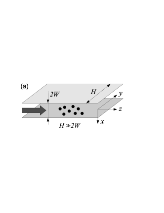
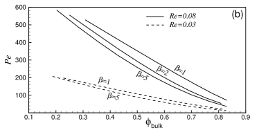
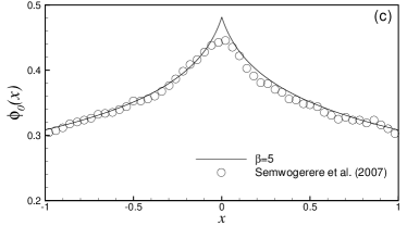
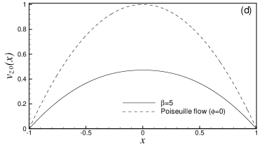
Figure 1: (a) Channel geometry; big arrow indicates flow direction. (b) Variation of Pe versus $\phi_{\rm bulk}$ for several choices of Re and $\beta$. We have set $K_{c}=0.03$. (c) Steady-state solution of the normalized particle concentration $\phi$ for $\beta=5$. Circles show the experimental results of Semwogerere et al. (2007, figures 3). (d) Solid line: the velocity profile $v_{z0}(x)$ corresponding to $\phi_{0}(x)$; dashed line: the velocity profile of Poiseuille flow in the limit of $\phi=0$. Model parameters are $K_{c}=0.03$, $\phi_{0}(\pm 1)=0.21/\phi_{m}$, $W=25\mu{\rm m}$, $a=0.7\mu{\rm m}$, $V_{p}=2.1\times 10^{-3}$m/s, $T=22^{\circ}$, $\eta_{s}=2.18\times 10^{-3}$Pa.s, $\rho=1232.5$kg/m³ and $D=8.4\times 10^{-2}$. The actual velocity is computed as $V_{p}v_{z0}(x)$. Using these parameters, we obtain $Q=16.92$ nl/s, $\mbox{{Pe}}=137$ and $\phi_{\rm bulk}=0.25/\phi_{m}$.

We have used the solution of (5) and plotted Pe versus $\phi_{\rm bulk}$ in figure 1(b) for several choices of Re and $\beta$. Figures 1(c) and 1(d) show the steady-state solutions of a suspension flow with $\beta=5$. The material and geometrical parameters—given in the figure caption—of this example come from Semwogerere et al. (2007) for the solvent cyclohexylbromide/decalin mixture. Using an evolution parameter, they have confirmed the steady state condition of the flow. We find $\phi_{\rm bulk}=0.25/\phi_{m}$ and $\mbox{{Pe}}=137$, which agree with the experimental data within 5% (see Semwogerere et al., 2007, figures 3 and 10c). The solid line in figure 1(c) accurately reproduces the concentration profile in figure 10(c) of Semwogerere et al. (2007) whose own analytical predictions (see also Morris & Boulay, 1999; Miller & Morris, 2006) show remarkable deviations from the measurements at the fully developed stage. This can be due either to electrical stresses, or particle random walks. The impressive match between the results of the steady-state model (5) and experimental data is mainly due to $D\not=0$ and supports the latter possibility. The significance of having a non-zero $D$ had not already been discussed/explored in the original work of Phillips et al. (1992) because they worked with very large Péclet numbers of ${\cal O}(10^{5})$.

2.2 Perturbed equations and eigenvalue problem

The steady concentration of particles in microchannels can easily be disturbed. For instance, unavoidable surface roughness, sedimentation, particle-wall and particle-particle interactions near a wall can induce small amplitude fluctuations on the boundary values of $\phi$ and generate global modes. To understand the transient response of suspensions, we carry out a linear stability analysis by perturbing the concentration and velocity fields as $\phi=\phi_{0}(x)+\tilde{\phi}(x,z,t)$ and $\textit{{v}}=v_{z0}(x)\textit{{e}}_{z}+\tilde{\textit{{v}}}(x,z,t)$. The magnitude of the shear rate and the normalized viscosity then become $\Gamma=\Gamma_{0}(x)+\tilde{\Gamma}(x,z,t)$ and $\eta=\eta_{0}(x)+\eta_{,\phi}(\phi_{0}(x))\,\tilde{\phi}$, where $\tilde{\Gamma}={\rm sign}\left(\partial v_{z0}/\partial x\right)\left(\tilde{v}_{x,z}+\tilde{v}_{z,x}\right)$. It is remarked that the transient response can develop structures in the $y$-direction as well. Since the steady-state quantities do not depend on $y$, the linear response in that direction will include a simple harmonic waveform with a wavelength $\ell_{y}$. The magnitudes of all gradients in the $y$-direction are determined by $1/\ell_{y}$. This study is conducted in the long wavelength limit $\ell_{y}\to\infty$.

The perturbed equations are simplified by assuming the stream function $\psi=\psi_{0}(x)+\tilde{\psi}(x,z,t)$ to express the velocity field: $\textit{{v}}=(\psi_{,z},-\psi_{,x})$. This implies $\textit{{v}}_{0}(x)=(0,-\psi_{0,x})$ and $\tilde{\textit{{v}}}=(\tilde{\psi}_{,z},-\tilde{\psi}_{,x})$, and the continuity equation is satisfied automatically both in the steady and perturbed states. We now take the curl of (4) and remove the pressure $p$ from computations. The resulting equation together with (1) are linearized to obtain:

$${\cal L}_{11}\tilde{\psi}+{\cal L}_{12}\tilde{\phi} = \mbox{{Re}}\left(\nabla^{2}\tilde{\psi}_{,t}+\psi_{0,xxx}\tilde{\psi}_{,z}-\nabla^{2}\tilde{\psi}_{,z}\right),$$ (6)

$$-\epsilon\nabla\cdot(\tilde{J}_{x}\textit{{e}}_{x}+\tilde{J}_{z}\textit{{e}}_{z}) = \tilde{\phi}_{,t}+\phi_{0,x}\tilde{\psi}_{,z}-\psi_{0,x}\tilde{\phi}_{,z},$$ (7)

where the perturbed components of the flux vector defined as $\tilde{J}_{x}={\cal L}_{21}\tilde{\psi}+{\cal L}_{22}\tilde{\phi}$ and $\tilde{J}_{z}={\cal L}_{31}\tilde{\psi}+{\cal L}_{32}\tilde{\phi}$. The linear operators ${\cal L}_{ij}$ are functions of $\psi_{0}(x)$, $\phi_{0}(x)$ and their $x$-derivatives. They are obtained by evaluating

$$\begin{array}[]{lll}{\cal L}_{11}=\left(\nabla\times\nabla\cdot\textsf{{T}}\right)_{,\tilde{\psi}},&{\cal L}_{12}=\left(\nabla\times\nabla\cdot\textsf{{T}}\right)_{,\tilde{\phi}},&{\cal L}_{21}=\left(\textit{{J}}\cdot\textit{{e}}_{x}\right)_{,\tilde{\psi}},\\ {\cal L}_{22}=\left(\textit{{J}}\cdot\textit{{e}}_{x}\right)_{,\tilde{\phi}},&{\cal L}_{31}=\left(\textit{{J}}\cdot\textit{{e}}_{z}\right)_{,\tilde{\psi}},&{\cal L}_{32}=\left(\textit{{J}}\cdot\textit{{e}}_{z}\right)_{,\tilde{\phi}},\end{array}$$ (10)

at $(\tilde{\psi},\tilde{\phi})=0$. The partial derivatives $\partial/\partial\nu$ and $\partial/\partial g$ are noncommutative over the extended space $(\nu,g)$ when $\nu\equiv(x,z,t)$ and $g\equiv(\tilde{\psi},\tilde{\phi})$ are independent and dependent variables, respectively. We have applied the rule $[f(\nu)g(\nu)]_{,\nu g}=f\partial/\partial\nu+\partial f/\partial\nu$ to calculate the partial derivatives in (10); i.e., we first differentiate with respect to independent variables, then perform the partial differentiations $\partial/\partial\tilde{\psi}$ and $\partial/\partial\tilde{\phi}$. The boundary conditions associated with the perturbed equations are $\tilde{\textit{{v}}}(\pm 1,z,t)=0$ and $\tilde{J}_{x}(\pm 1,z,t)=0$. It is remarked that $\tilde{J}_{z}(\pm 1)$ can vary arbitrarily.

We consider $\tilde{\psi}(x,z,t)=\exp({\rm i}kz-{\rm i}\omega t)\Psi(x)$ and $\tilde{\phi}(x,z,t)=\exp({\rm i}kz-{\rm i}\omega t)\Phi(x)$, where $\omega=\Omega+\zeta\,{\rm i}$ (${\rm i}=\sqrt{-1}$) and $\ell_{z}=2\pi/k$ is the wavelength of oscillations along the channel. $\Omega=2\pi/(\lambda t_{B})=2\pi D/\lambda$ is the wave frequency and $\zeta$ is the growth/decay rate. Short-period transient oscillations with $\lambda\ll 1$ are dissolved by thermal fluctuations. Therefore, only long-period oscillations of $\lambda\gtrsim 1$ can exist. The linear solutions are decoupled in the $k$-space, and equations (6) and (7) remain invariant under the transformation $x\to-x$ if $\tilde{\psi}(x,z,t)=\mp\tilde{\psi}(-x,z,t)$ and $\tilde{\phi}(x,z,t)=\pm\tilde{\phi}(-x,z,t)$. This means that both symmetric and anti-symmetric modes are supported by the governing equations, and that degenerate pairs may exist in the eigenspectrum of $\omega$. Equation (6) reduces to Orr-Sommerfeld stability equation when $\phi=0$.

Most microchannels have typical widths of $2W\sim 10^{-4}$m. For $a\sim 10^{-6}$m, we will get $\epsilon\sim{\cal O}(10^{-5})$ and $0.01\lesssim\mbox{{Re}}\lesssim 1$. On the other hand, the response time of $\tilde{\phi}$ to particle migrations is scaled by $\epsilon$, which is understood from equation (7). Therefore, the growth/decay rates of modes supported by diffusion, and not by the perturbations of streamlines, can be as small as $\zeta\sim{\cal O}(\epsilon)\sim 10^{-5}$, which requires a sophisticated numerical procedure to be resolved.

We utilise the Chebyshev tau algorithm (Orszag, 1971; Dongarra et al., 1996) to compute the wave functions $\Psi(x)$ and $\Phi(x)$, and assume $\Psi(x)=\sum p_{n}T_{n}(x)$ and $\Phi(x)=\sum q_{n}T_{n}(x)$ where $T_{n}(x)$ are Chebyshev polynomials defined over the region $-1\leq x\leq+1$. There are six boundary conditions associated with $\tilde{\psi}$ and $\tilde{\phi}$. This suggests to assume six new unknowns, the so-called $\tau$ variables. Introducing a complex vector z, which contains the variables $p_{n}$, $q_{n}$ ($n=0,1,\cdots,N$) and $\tau_{j}$ ($j=1,2,\cdots,6$), and the Galerkin weighting of (6) and (7), leave us with the linear eigensystem $\textsf{{A}}\cdot\textit{{z}}=\omega\textsf{{B}}\cdot\textit{{z}}$ where A and B are complex matrices. In our implementation of the Chebyshev tau method, we use the formula $d^{m}T_{n}(x)/dx^{m}=2^{m-1}n(m-1)!\,C^{m}_{n-m}(x)$ (Gradshteyn & Ryzhik, 2007) where $C^{m}_{n-m}(x)$ are Gegenbauer polynomials. We find the generalized complex eigenvalues $\omega$ and their associated right eigenvectors using the routine zggev.f of LAPACK library. We begin our calculations with $N=20$ and increase $N$ until $\min[|\Omega|,|\zeta|]$ converges within $0.5\%$ for the mode with the smallest $|\zeta|$ in the spectrum. The major source of errors is the numerical evaluation of the inner products $\langle T_{n^{\prime}},{\cal L}_{ij}T_{n}\rangle$, especially when the derivatives of $\phi_{0}(x)$ and $\Gamma_{0}(x)$ with jump discontinuities at $x=0$ appear in the integrand. We compute the inner products using a mid-point rule to avoid $x=0$, and use finer grids in the $x$-domain as $n$ or $n^{\prime}$ increase. A uniform grid helps us simultaneously resolve the strong near-wall features of certain modes and handle the central cusp. Reaching to $0.5\%$ error threshold occasionally needs $N\gtrsim 80$ to capture short wavelength modes when $\zeta\sim{\cal O}(\epsilon)$. To calibrate our code, we have solved the Orr-Sommerfeld stability equation and reproduced the results of Orszag (1971) up to the 8th decimal place. To assure that the physical eigenfrequencies are not sensitive to the choice of basis functions, we used Fourier series to reconstruct $\Phi(x)$ and $\Psi(x)$, and compared the resulting spectra with Chebyshev tau algorithm. The results of two methods match very well for modes that peak near the channel centreline. The Chebyshev tau method, however, gives more accurate results for modes that develop bumps near the walls. Our numerical calculations show that Fourier series increase the number of spurious modes.

Mode	$D$	0Pe	Re	$\phi_{m}\phi_{\rm bulk}$	$k$	0$\beta$	$\omega^{\uparrow\downarrow}=\Omega+\zeta\,{\rm i}$	$\omega^{\uparrow\uparrow}=\Omega+\zeta\,{\rm i}$
${\rm S}1,{\rm S}2$	0$0.084$	0137	0.03	0.24	1.0	05	0$0.017958-0.010418\,{\rm i}$	0$0.017886-0.010543\,{\rm i}$
${\rm S}3$	0$0.084$	0137	0.03	0.24	1.0	05	0$0.482467-0.000397\,{\rm i}$
${\rm S}4$	0$0.084$	0137	0.03	0.24	1.0	05		0$0.471442-0.000425\,{\rm i}$
${\rm U}1,{\rm U}2$	0$0.030$	053.5	0.08	0.55	0.1	02	0$0.000844+0.000282\,{\rm i}$	0$0.000851+0.000303\,{\rm i}$
${\rm U}3$	0$0.030$	053.5	0.08	0.55	0.1	02		0$0.006675+0.000053\,{\rm i}$

Table 1: Eigenfrequencies of long-lived and unstable modes for a suspension flow with $K_{c}=0.03$ and $\epsilon=1.6\times 10^{-5}$. Degenerate pairs appear in a single row. The shape of each mode is identified through the symmetric (^↑↑) or anti-symmetric (^↑↓) shape of $\Phi(x)$.

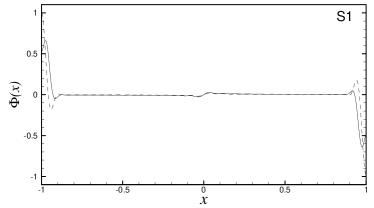
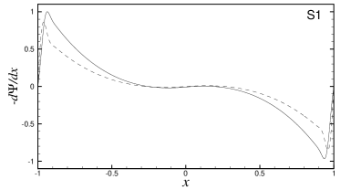
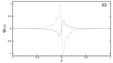
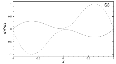
Figure 2: The wave functions $\Phi(x)$ (left) and $-d\Psi(x)/dx$ (right) for the long-lived modes S1 (top row) and S3 (bottom row). Note the strong near-wall features of mode S1. This property is also shared by its symmetric partner S2. Solid and dashed lines correspond to the real and imaginary parts of the wave functions.

3 Long-lived and unstable modes

We first carry out the stability analysis for the steady $\beta=5$ model of §2.1 (see figure 1). The main properties of this model, which we call model A, are (i) relatively low $\phi_{\rm bulk}$; (ii) almost no flattening of the velocity profile near the channel centreline. The matrices A and B depend explicitly on $\epsilon$ and Re. In the limit $\epsilon=0$, the evolution of $\tilde{\phi}$ is only dictated by the deformations of streamlines, and we find only highly-damped, stable discrete modes ($\zeta\ll-1$), which are the characteristics of incompressible Newtonian flows at low Reynolds regimes. Turning on the effect of particle migration, $\epsilon\not=0$, gives birth to new long-lived modes with $-1\ll\zeta<0$. The eigenfrequencies of long-lived modes have been calculated for $k=1$ and given in Table 1. These modes belong to two general families: degenerate and single modes. The oscillation periods and decay rates of modes S1 and S2 are $\approx 26$ times larger than those of modes S3 and S4. We have plotted $\Phi(x)$ and the $x$-dependent part of $\tilde{v}_{z}(x,z,0)=-\exp({\rm i}kz)d\Psi(x)/dx$ in figure 2 for modes S1 and S3. It is seen that the concentration profile of mode S1 has strong peaks near the walls while the dominant peaks of mode S3 have been generated near the channel centreline. Modes S1 and S2 have a better chance for being excited because particle-wall interactions can easily disturb the particle concentration and velocity field near the wall. Modes S3 and S4 are most likely due to collective random motions because they have small periods of $\approx 1.1\,t_{B}$ with $\Omega_{\rm S1}/\Omega_{\rm S3}\sim{\cal O}(D)$, decay slowly so that $\zeta_{{\rm S}_{3}}/\zeta_{{\rm S}_{1}}\sim{\cal O}(D)$, and have wide-spread patterns. S1 and S2 are therefore viscous modes supported by SID.

We now define the actual decay time of mode X as $t^{\rm X}_{d}=-(W/V_{p})\ln(0.1)/\zeta_{\rm X}$, which is the duration that the amplitude of $\tilde{\phi}$ decays to 10% of its initial value. The actual oscillation period of mode X is given by $t^{\rm X}_{p}=(W/V_{p})\lambda_{\rm X}t_{B}$. We find $(t^{\rm S1}_{d},t^{\rm S1}_{p})=(2.63\,{\rm s},4.16\,{\rm s})$. The characteristic times of mode S3 are quite surprising: $(t^{\rm S3}_{d},t^{\rm S3}_{p})=(69.05\,{\rm s},0.15\,{\rm s})$, which indicate an almost quasi-stationary oscillation in laboratory scales. All these modes will exhibit a high signal to noise ratio and can be measured by currently available high-speed imagers. The detection of S1 and S2 requires high spatial resolution, while S3 and S4 need high frame rates due to their small periods. The ripples in the concentration profiles, and the near-wall excess/deficit of particles observed in experiments (see Frank et al., 2003; Semwogerere et al., 2007; Semwogerere & Weeks, 2008; Brown et al., 2009) might be long-lived modes. Since $\zeta_{\rm S3}\approx\zeta_{\rm S4}$, we anticipate the coexistence of modes S3 and S4. The small difference between their frequencies can yield a quasi-periodic oscillation.

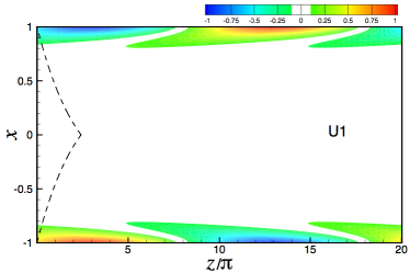
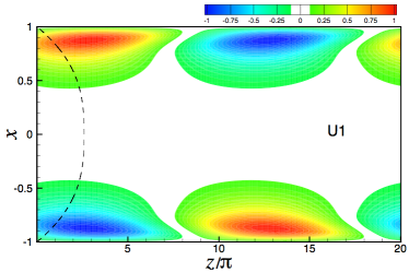
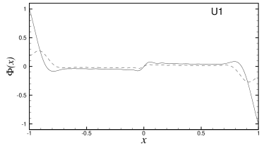
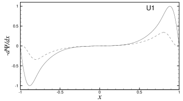
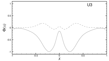
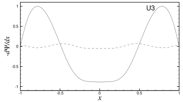
Figure 3: The shapes of the unstable modes U1 and U3. Top panels demonstrate the contour plots of $\tilde{\phi}$ (left) and $\tilde{v}_{z}$ (right) at $t=0$ for mode U1. Dashed lines in the panels of $\tilde{\phi}$ and $\tilde{v}_{z}$ show, respectively, the forms of the associated steady solutions $\phi_{0}(x)$ and $v_{z0}(x)$. The blank region corresponds to the lowest $10\%$ of the mode magnitude, which has not been shaded to highlight the major near-wall features. Middle and bottom panels show the wave functions $\Phi(x)$ (left) and $-d\Psi(x)/dx$ (right) for modes U1 and U3, respectively. Solid and dashed lines correspond to the real and imaginary parts of the wave functions.

Increasing $\phi_{\rm bulk}$ has a significant influence on the velocity profile and flattens it near the channel centreline (e.g., Semwogerere et al., 2007, figure 4). Our calculations show that in models with $\phi(0)<1$ the flattening of the steady velocity curve is mainly controlled by the parameter $\beta$. The flattening of $v_{z0}(x)$ at $x=0$ is quantified by the curvature ${\cal C}=v_{z0,xx}(0)$, which equals $-2$ for Poiseuille flow. To investigate the effect of ${\cal C}$ on the stability of suspension flows, we build another model B, and increase the average concentration to $\phi_{\rm bulk}=0.55/\phi_{m}$. We then set $V_{p}=6\times 10^{-3}$m/s and $\beta=2$ to obtain a mass flow rate $Q=7\,{\rm nl/s}$. In this new flow regime, the curvature at $x=0$ becomes ${\cal C}=-0.02235$ indicating a significant flattening. The perturbed equations now result in three unstable modes (U1, U2 and U3) with $\zeta>0$. They have been reported in Table 1 for $k=0.1$ ($\ell_{z}=20\pi$). We have used this particular long wavelength because it expands the wavelengths of $\Phi(x)$ and $\Psi(x)$ in the $x$-direction, and leads to more visible patterns.

Unstable modes U1 and U2 are degenerate pairs, and U3 is a single symmetric mode. Modes U1 and U2 are the counterparts of S1 and S3. The oscillation periods of long wavelength unstable modes are: $t^{\rm U1}_{p}=31$, $t^{\rm U2}_{p}=30.76$ and $t^{\rm U3}_{p}=3.92$ seconds, and their amplitudes are magnified by a factor of 10 within $32$–$34$ seconds for the degenerate pair and $181.7$ seconds for mode U3. The dominant concentration and velocity peaks of modes U1 and U2 are developed near the channel wall (figure 3). The likelihood of exciting these modes is thus very high because of sedimentation or particle-wall interactions. In figure 3, we have also demonstrated the contours of $\mbox{Re}[\tilde{\phi}]=\mbox{Re}[\exp({\rm i}kz-{\rm i}\omega t)\,\Phi(x)]$ and $\mbox{Re}[\tilde{v}_{z}]=\mbox{Re}[-\exp({\rm i}kz-{\rm i}\omega t)\,d\Psi(x)/dx]$ for mode U1 at $t=0$. Prominent curved tails have been developed in the wave packets of both $\tilde{\phi}$ and $\tilde{v}_{z}$. These features are shared by Kelvin-Helmholtz type instabilities that are usually triggered at interfaces, but our modes have emerged between the central region (where particles move with an almost constant velocity) and highly-sheared zone near the walls.

The channel flow of suspensions with spherical particles involves five parameters (Re, Pe, $\phi_{0}(0)$, $\beta$ and $D$) and it is impractical to survey the entire parameter space and identify its unstable zone. Here we vary only $\beta$, which also controls Pe and the normalized average concentration $\phi_{\rm bulk}$, and attempt to understand how the gradients of $\phi_{0}(x)$ and $v_{z0}(x)$ near the channel centreline (see §2.1) correlate with the instability. We find that by decreasing $\beta$ in model A, the magnitude of $\zeta$ drops for all modes until mode S3 becomes unstable for $\beta\lesssim 1.8$ ($\mbox{{Pe}}\approx 124.3$, $\phi_{\rm bulk}\approx 0.29/\phi_{m}$). Other modes (S1, S2, and S4) are destabilized by further decreasing $\beta$. In another experiment, we gradually increased $\beta$ in the initially unstable model B to obtain more cuspy concentrations and less flattened velocity profiles as $|x|\to 0$. We find that mode U3 is stabilized for $\beta\gtrsim 4.5$ ($\mbox{{Pe}}\approx 65.4$, $\phi_{\rm bulk}\approx 0.52/\phi_{m}$). Modes U1 and U2 resist stabilization until $\beta\approx 4.8$. It is seen that Pe should decrease though mildly and $\phi_{\rm bulk}$ should increase to get instability. Nonetheless, both stable and unstable modes exist for $53\lesssim\mbox{{Pe}}\lesssim 124$, $0.42\lesssim\phi_{\rm bulk}\lesssim 0.8$ and $1.8\lesssim\beta\lesssim 4.8$. The only property shared by all unstable systems is the flattened velocity profile, which constitutes a ‘necessary’ condition for instability.

Varying the wavelength $\ell_{z}=2\pi/k$ has also a notable impact on eigenfrequencies. Our calculations show that $\Omega$ and $|\zeta|$ increase proportional to $k$ in both the stable and unstable models. i.e., unstable modes grow faster for shorter wavelengths. Moreover, we find that the wavelengths of $\Phi(x)$ and $-d\Psi(x)/dx$ are approximately proportional to $\ell_{z}$, and consequently, the wave packets of degenerate modes become more compact near the walls for larger values of $k$ (compare the graphs of $-d\Psi(x)/dx$ in figures 2 and 3). All these suggest that short wavelength instabilities can rapidly ruin the flow structure in the vicinity of the walls. Modes with longer wavelengths and lower oscillation frequencies can survive far from the walls and be observed experimentally. In a full three dimensional excitation with $\ell_{y}<\infty$, we anticipate faster growth and oscillation of unstable modes because clumps in the $y$-direction can probably enhance the migration of particles.

To this end, we argue that unstable modes U1 and U2 are amplified by the Brownian motion of particles. For a relatively low Pe and due to Brownian diffusion, some particles can ‘leak’ from the region with flat velocity curve and move towards the channel walls. Such particles will locally increase the volume fraction and viscosity, while the suspension velocity drops. Note that the positive bumps of $\tilde{\phi}$ and $\tilde{v}_{z}$ are out of phase in the upper panels of figure 3. Particles initially moving close to the channel walls can also penetrate to inner regions through Brownian diffusion. When the overall velocity profile, $v_{z0}(x)+\tilde{v}_{z}(x,z,t)$, is flat near the channel centreline, SID cannot efficiently disperse particles trapped in the cavities of $(\tilde{\phi},\tilde{\textit{{v}}})$. Sustained Brownian migration, back and forth between highly-sheared and central regions, thus amplifies the concentration and velocity anomalies and triggers a mode. This instability mechanism works for mode U3 as well because the shape of $\tilde{v}_{z}$ is sufficiently flat in central regions (bottom panels in figure 3). Modes will be damped when SID becomes dominant due to the steady form of $\Gamma_{0}(x)$. In this condition SID will disperse particles participating in perturbations, and facilitate their migration towards the channel centre. This is why the transition from unstable to stable modes strongly correlates with the value of $\beta$, which controls the flatness of velocity curve.

4 Conclusions

We showed that the steady-state solutions of the model of Phillips et al. (1992) can reproduce recent experimental results of Brownian suspensions with spherical particles. We calculated the eigenmodes of the corresponding perturbed equations, and found new families of long-lived and unstable modes. Unstable modes that we find occur when the fully-developed velocity profile is sufficiently flattened near the channel centreline. The fastest growing modes appear as degenerate pairs, and they live inside the highly-sheared region near the walls. Since our model has not taken particle-wall interactions into account, unstable modes seem to be triggered by the transverse Brownian migrations across the streamlines of the fully developed flow. Mode amplification in models with flattened velocity profiles is mainly due to inefficient shear-induced diffusion that can, in principle, disperse particles and force them to move towards the channel centreline. Rapidly growing unstable modes destruct the flow structure near the walls, and they can explain the experimentally observed excess and/or deficit of particles near the channel walls. The instability mechanism that we suggested operates along the shortest direction of the channel. Therefore, dynamics along the neglected $y$-direction may only affect the wavelength and period of developing patterns, and not their general shapes. The three dimensional response of Brownian suspensions, especially in channels with $2W\sim H$, requires further exploration.

We thank Howard Stone for his insightful comments. A.K. thanks the department of Mechanical and Aerospace Engineering at Princeton University for their hospitality and generous support. We are indebted to anonymous referees whose criticisms helped us to substantially improve the presentation of the paper.

References

- Brown et al. (2009) Brown, J. R., Fridjonsson, E. O., Seymour, J. D. & Codd, S. L. 2009 Nuclear magnetic resonance measurement of shear-induced particle migration in Brownian suspensions. Phys. of Fluids 21, 093301
- Carpen & Brady (2002) Carpen, I. C. & Brady, J. F. 2002 Gravitational instability in suspension flow. J. Fluid Mech. 472, 201-210
- Dongarra et al. (1996) Dongarra, J. J., Straughan, B. & Walker, D. W. 1996 Chebyshev tau/QZ algorithm methods for calculating spectra of hydrodynamic stability problems. Journal of Applied Numerical Mathematics 22, 399-435
- Frank et al. (2003) Frank, M., Anderson, D., Weeks, E. R. & Morris, J. F. 2003 Particle migration in pressure-driven flow of a Brownian suspension. J. Fluid Mech. 493, 363-378
- Govindarajan et al. (2001) Govindarajan, R., Nott, P. R. & Ramaswamy, S. 2001 Theory of suspension segregation in partially filled horizontal rotating cylinders. Phys. Fluids 13, 3517-3520
- Gradshteyn & Ryzhik (2007) Gradshteyn, I.S. & Ryzhik, I.M. 2007 Table of Integrals, Series, and Products. Seventh Edition, Academic Press, Amsterdam
- Helton & Yager (2007) Helton, K. L. & Yager, P. 2007 Interfacial instabilities affect microfluidic extraction of small molecules from non-Newtonian fluids. Lab Chip 7, 1581-1588
- Kauzlarić et al. (2011) Kauzlarić, D., Pastewka, L., Meyer, H., Heldele, R., Schulz, M., Weber, O., Piotter, V., Hausselt, J., Greiner, A. & Korvink, J. G. 2011 Smoothed particle hydrodynamics simulation of shear-induced powder migration in injection moulding. Phil. Trans. R. Soc. A 369, 2320-2328
- Klinkenberg et al. (2011) Klinkenberg, J., de Lange, H. C. & Brandt, L. 2011 Modal and non-modal stability of particle-laden channel flow. Phys. of Fluids 23, 064110
- Kromkamp et al. (2006) Kromkamp, J., van der Padt, A., Schroen, C. G. P. H. & Boom, R. M. 2006 Shear induced fractionation of particles. Patent EP1 673 957 A1, European Patent Office
- Leighton & Acrivos (1987) Leighton, D. & Acrivos, A. 1987 The shear-induced migration of particles in concentrated suspensions. J. Fluid Mech. 181, 415-439
- Merhi et al. (2005) Merhi, D., Lemaire, E., Bossis, G. & Moukalled, F. 2005 Particle migration in a concentrated suspension flowing between rotating parallel plates: Investigation of diffusion flux coefficients. J. Rheol 49, 1429-1448
- Miller & Morris (2006) Miller, R. M. & Morris J. F. 2006 Normal stress-driven migration and axial development in pressure-driven flow of concentrated suspensions. J. Non-Newtonian Fluid Mech. 135, 149 165
- Morris & Boulay (1999) Morris, J. F. & Boulay F. 1999 Curvilinear flows of noncolloidal suspensions: The role of normal stresses. J. Rheol. 43, 1213-1237
- Nott & Brady (1994) Nott, P. R. & Brady, J. F. 1994 Pressure-driven flow of suspensions: simulation and theory. J. Fluid Mech. 275, 157-199
- Orszag (1971) Orszag, S. A. 1971 Accurate solution of the Orr-Sommerfeld stability equation. J . Fluid Mech. 50, 689-703
- Phillips et al. (1992) Phillips, R. J., Armstrong, R. C. & Brown, R. A. 1992 A constitutive equation for concentrated suspensions that accounts for shear-induced particle migration. Phys. Fluids 4, 30-40
- Rao et al. (2007) Rao, R. R., Mondy, L. A. & Altobelli, S. A. 2007 Instabilities during batch sedimentation in geometries containing obstacles: A numerical and experimental study. Int. J. Numer. Meth. Fluids 55, 723-735
- Rudyak et al. (1997) Rudyak, V. Ya., Isakov, E. B. & Bord, E. G. 1997 Hydrodynamic stability of the Poiseuille flow of dispersed fluid. J. Aerosol Sci. 28, 53-66
- Rusconi & Stone (2008) Rusconi, R. & Stone, H. A. 2008 Shear-induced diffusion of platelike particles in microchannels. Phys. Rev. Lett. 101, 254502
- Semwogerere et al. (2007) Semwogerere, D., Morris, J. F. & Weeks, E. R. 2007 Development of particle migration in pressure-driven flow of a Brownian suspension. J. Fluid Mech. 581, 437-451
- Semwogerere & Weeks (2008) Semwogerere, D. & Weeks, E. R. 2008 Shear-induced particle migration in binary colloidal suspensions. Phys. Fluids 20, 043306
- Stickel & Powell (2005) Stickel, J. J. & Powell, R. L. 2005 Fluid mechanics and rheology of dense suspensions. Annual Review of Fluid Mechanics 37, 129-149
- Vollebregt et al. (2010) Vollebregt, H. M., van der Sman, R. G. M. & Boom, R. M. 2010 Suspension flow modelling in particle migration and microfiltration. Soft Matter 6, 6052-6064
- Yurkovetsky & Morris (2008) Yurkovetsky, Y. & and Morris, J. F. 2008 Particle pressure in sheared Brownian suspensions. J. Rheol. 52, 141-164
- Yiantsios (2006) Yiantsios, S. G. 2006 Plane Poiseuille flow of a sedimenting suspension of Brownian hard-sphere particles: Hydrodynamic stability and direct numerical simulations. Phys. of Fluids 18, 054103