Discrete multi-colour random mosaics with an application to network extraction

We introduce a class of random fields that can be understood as discrete versions of multi-colour polygonal fields built on regular linear tessellations. We focus first on consistent polygonal fields, for which we show Markovianity and solvability by means of a dynamic representation. This representation forms the basis for new sampling techniques for Gibbsian modifications of such fields, a class which covers lattice based random fields. A flux based modification is applied to the extraction of the field tracks network from a SAR image of a rural area.
2010 Mathematics Subject Classification: 60D05, 60G60.
Keywords: consistent polygonal field, dynamic representation, linear network extraction, random field.

In memory of Tomasz F. Schreiber.

1 Introduction

In the 1980s, Arak and Surgailis introduced a class of planar Markov fields whose realisations form a coloured tessellation of the plane. The basic idea is to use the lines of an isotropic Poisson line process as a skeleton on which to draw polygonal contours with the restriction that each line cannot be used more than once. Note that many tessellations can be drawn on the same skeleton and that the contours may be nested. The polygons are then coloured randomly subject to the constraint that adjacent ones must have different colours. Formally, the probability distribution of such polygonal Markov fields is defined in terms of a Hamiltonian with respect to the law of the underlying Poisson line process, which can be chosen in such a way that many of the basic properties of the Poisson line process (including consistency, Poisson line transects, and an explicit expression for its probability distribution on the hitting set of bounded domains) carry over and a Markov property holds. Another useful feature is that a dynamic representation in terms of a particle system is available. See [2, 3] for further details and [4] or [27] for alternative point rather than line based models. The special case where all vertices have degree three was studied in [16].

The simplest and most widely studied example of a planar Markov field is the Arak process [1] which consists of self-avoiding closed polygonal contours. Hence interaction is restricted to a hard core condition on the contours, and there are exactly two colourings using the labels ‘black’ and ‘white’ such that adjacent polygons have different colours. For the Arak process, the Hamiltonian is proportional to the total contour length by a factor two. One may introduce further length-interaction by changing the proportionality constant. Doing so, Nicholls [18] and Schreiber [21] consider the separation between the black and white regions as the interaction gets stronger; Van Lieshout and Schreiber [14] develop perfect simulation algorithms for these models. For the more general case in which both length and area terms feature in the Hamiltonian, Schreiber [20] proposes a Metropolis–Hastings scheme based on the dynamic representation of the Arak process, which Kluszczyński et al. [11] adapt and implement to solve foreground/background image segmentation problems. An anisotropic Arak process can be defined through local activity functions instead of the length functional [22, 24] and allows for increased flexibility while preserving desirable basic properties including a dynamic representation. This representation forms the basis of a stochastic optimisation algorithm in the context of image segmentation, implemented by Matuszak and Schreiber [17], and helps to gain insight into the higher order correlation structure [22].

Polygonal Markov field models with contours that may also be joined by a vertex of degree three or four [2, 3] are much less well-understood due to the more complicated interaction structure. Papers in this direction include [7, 12, 19].

In a previous paper [23], we introduced a class of binary random fields that can be understood as discrete counterparts of the two-colour Arak process. The aim of the present paper is to extend this construction to allow for an arbitrary number of colours and to relax the assumption in [23] that no polygons of the same colour can be joined by corners only. Our construction is two-staged: first a collection of lines is fixed to serve as a skeleton for drawing polygonal contours (a regular lattice being the generic example), then the resulting polygons are coloured in such a way that adjacent ones do not have the same colour. The analogy with continuum polygonal Markov fields is exploited to define Hamiltonians that are such that the desirable properties of these processes mentioned above hold. Moreover, we propose new simulations techniques that combine global changes with the usual local update methods employed for random fields on finite graphs [29]. It should be stressed, though, that the discrete models considered in this paper are not versions of continuum polygonal Markov fields conditioned on having their edges fall along a given finite collection of lines.

The plan of this paper is as follows. In Section 2 we define a family of admissible multi-colour polygonal configurations built on regular linear tessellations, and define discrete polygonal fields with special attention to consistent ones. In Section 3 we present a dynamic representation of consistent polygonal fields, which is used to prove the main properties of such models. In Section 4, we exploit the dynamic representation to develop a simulation method for consistent polygonal fields. The method is generalised to arbitrary Gibbs fields with polygonal realisations and applied to the detection of linear networks in images in Section 5. We conclude with a discussion.

2 Random fields with polygonal realisations

First, recall the definition of a regular linear tessellation from [23].

Definition 1.

A regular linear tessellation of the plane is a countable family ${\cal T}$ of straight lines in ${{\mathbb{R}}}^{2}$ such that no three lines of ${\cal T}$ intersect at one point and such that any bounded subset of the plane is hit by at most a finite number of lines from ${\cal T}$.

For a bounded open convex set $D$, ${\cal T}$ induces a partition of $D$ into a finite collection $D_{\cal T}$ of convex cells of polygonal shapes, possibly chopped off by the boundary. Below we shall always assume that the boundary $\partial D$ of $D$ contains no intersection points of lines from ${\cal T}$ and that the intersection of each line $l\in{\cal T}$ with $\partial D$ consists of exactly two points. To each line $l$, we ascribe a fixed activity parameter $\pi_{l}\in(0,1)$ to allow for the possibility to favour some lines over others.

The next step is to assign a colour to each of the convex cells in the partition of $D$ induced by the lines in ${\cal T}$. Write $\{1,\dots,k\}$ for the set of colour labels. In this paper, we concentrate on the case that $k>2$. Such a colouring gives rise to a graph whose edges are formed by the boundaries between cells that have been assigned different colours. For technical convenience, we shall assume that edges are open, that is, they do not contain the vertices in which they intersect. Faces of the graph, which are unions of cells of $D_{\cal T}$, are said to be adjacent if they share a common edge.

Definition 2.

The family $\hat{\Gamma}_{D}({\cal T})$ of admissible coloured polygonal configurations in $D$ built on ${\cal T}$ consists of all coloured planar graphs $\hat{\gamma}$ in the topological closure $\overline{D}=D\cup\partial D$ of $D$ such that

• all edges lie on the lines of ${\cal T}$;

• all interior vertices, i.e. those lying in $D$, are of degree $2$, $3$ or $4$;

• all boundary vertices, i.e. those lying on $\partial D$, are of degree $1$;

• no adjacent faces share the same colour.

Throughout this paper, the notation $\gamma$ is used for (admissible) planar graphs and the hat notation $\hat{\gamma}$ for the graph with colours assigned to its faces. In this notation, $\Gamma_{D}({\cal T})$ stands for the family of all planar graphs $\gamma$ arising as interfaces between differently coloured faces in $\hat{\gamma}\in\hat{\Gamma}_{D}({\cal T})$. Note that for the case $k=2$ treated in [23], all interior vertices have degree two. Vertices of degree two are also known as V-vertices, those of degree three as T-vertices, and vertices of degree four as X-vertices.

To avoid confusion, it is important to distinguish between $D_{\cal T}$ and the members of $\Gamma_{D}({\cal T})$, even though they all partition $D$. In the sequel we shall reserve the terms ‘segments’ and ‘nodes’ for the former, ’edges’ and ’vertices’ for the latter. Thus, nodes are intersection points of lines in ${\cal{T}}$, which are joined by segments. Edges of $\gamma$ are maximal unions of connected collinear segments that are not broken by other such segments lying on the graph (corresponding to vertices of degree three or four). Primary edges are maximal unions of connected collinear segments, possibly consisting of multiple edges due to T- or X-vertices. Likewise, a vertex of $\gamma$ is a point where two edges of $\gamma$ meet or where an edge of $\gamma$ meets the boundary $\partial D$, nodes lying on the interior of graph edges are not considered to be vertices. These concepts are illustrated in Figure 1. The family ${\cal T}$ consists of two orthogonal line bundles and induces diamond shaped cells. One element of $\Gamma_{D}({\cal T})$ is plotted in Figure 1. Consider the polygonal face indicated by ‘C’ that is chopped off by the boundary. There are $2$ boundary vertices and $12$ interior vertices, $5$ of degree $2$, $7$ of degree $3$ and none of degree $4$. We count $17$ nodes on $16$ complete segments, with $2$ segments partly visible due to truncation by the boundary. $C$ has $13$ edges and its boundary lies on $8$ primary edges. Note that in the literature, primary edges are sometimes also known as sides. See e.g. [28] for a discussion on nomenclature for tessellations.

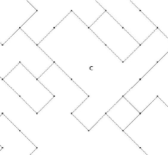
Figure 1: Admissible polygonal configuration.

We are now ready to define (discrete) polygonal fields.

Definition 3.

Let ${\cal T}$ be a regular linear tessellation and ascribe fixed activity parameters $\pi_{l}\in(0,1)$ to the lines $l\in{\cal T}$. For a function ${\cal H}_{D}:\hat{\Gamma}_{D}({\cal T})\mapsto{\mathbb{R}}\cup\{+\infty\}$, the (discrete) polygonal field $\hat{\cal A}_{{\cal H}_{D}}$ with Hamiltonian ${\cal H}_{D}$ is the random element in $\hat{\Gamma}_{D}({\cal T})$ such that

$${\mathbb{P}}\left(\hat{\cal A}_{{\cal H}_{D}}=\hat{\gamma}\right)=\frac{\exp(-{\cal H}_{D}(\hat{\gamma}))\prod_{e\in E^{*}(\gamma)}\pi_{l[e]}}{{\cal Z}[{\cal H}_{D}]}.$$ (1)

Here $E^{*}(\gamma)$ denotes the set of primary edges in $\gamma$ and $l[e]\in{\cal T}$ is the straight line containing the open edge $e$.

The constant

$${\cal Z}[{\cal H}_{D}]=\sum_{\hat{\theta}\in\hat{\Gamma}_{D}({\cal T})}\exp(-{\cal H}_{D}(\hat{\theta}))\prod_{e\in E^{*}(\theta)}\pi_{l[e]}$$ (2)

that ensures that ${\mathbb{P}}$ is a probability distribution is called the partition function. Note that the polygonal field is a Gibbs field with Hamiltonian

$${\cal H}_{D}(\hat{\gamma})-\sum_{e\in E^{*}(\gamma)}\log\pi_{l[e]}.$$

The terms $\log\pi_{l[e]}$ represent the energy needed to create the edges. We prefer to use the term polygonal field since the consistent fields to be considered shortly are inspired by the Arak–Surgailis polygonal Markov fields in the continuum, and, more importantly, because the graph-theoretical formulation leads us to define novel simulation techniques for discrete random fields.

A careful choice of Hamiltonian in (1) leads to consistent polygonal fields. Recall that $k$ is the number of colour labels.

Definition 4.

Let $\alpha_{V}\in[0,1]$ and set

$$\alpha_{X}=1-\alpha_{V};\quad\quad\alpha_{T}=\frac{1}{2}\left(1-\frac{k-2}{k-1}\alpha_{X}\right);\quad\quad\epsilon=\frac{\alpha_{V}}{k-1}+\frac{k-2}{k-1}\alpha_{T}.$$

The polygonal fields (1) defined by Hamiltonians of the form

$${\Phi}_{D}(\hat{\gamma}) = -N_{V}(\gamma)\log\alpha_{V}-N_{T}(\gamma)\log((k-1)\alpha_{T})-N_{X}(\gamma)\log((k-1)\alpha_{X})$$ (3)

$$+ {\rm{card}}(E(\gamma))\log(k-1)$$

$$- \sum_{e\in E(\gamma)}\sum_{l\in{\cal T},\;l\nsim e}\log(1-\epsilon\pi_{l})+\sum_{n(l_{1},l_{2})\in\gamma}\log\left(1-\frac{\alpha_{V}}{k-1}\pi_{l_{1}}\pi_{l_{2}}\right)$$

are referred to as consistent polygonal fields. Here, $N_{V}$, $N_{T}$ and $N_{X}$ denote the number of V-, T- and X-vertices, ${\rm{card}}(E(\gamma))$ is the number of edges in $\gamma$, $n(l_{1},l_{2})\in\gamma$ ranges through the nodes of ${\cal{T}}$ that either lie on edges of $\gamma$ or coincide with one of its vertices, and $l\nsim e$ means that the line $l$ intersects but is not collinear with $e$. We use the convention that $0\times\infty=0$.

A few remarks are in order. The parameter $\alpha_{V}$ controls the relative frequency of $V$-vertices, $\alpha_{T}$ and $\alpha_{X}$ that of vertices of degrees three and four respectively. These parameters are not independent and, given the number of colours $k$, $\alpha_{T}$ and $\alpha_{X}$ are uniquely determined by $\alpha_{V}$. This dependence will become more explicit in the dynamic representation to be derived in Section 3. Typical realisations for $k=3$ and $\alpha_{V}$ equal to $0$, $1/2$ and $1$ are shown in Figure 2. In the left-most panel, $\alpha_{V}=0$ and there no vertices having degree two; in the right-most panel, $\alpha_{X}=0$ so that no vertices have degree four. The central panel displays a coloured configuration with vertices of all degrees. Visually, the three patterns are strikingly different.

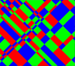
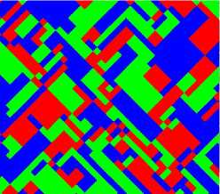
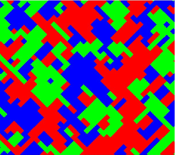
Figure 2: Realisations of $\hat{\cal{A}}_{\Phi_{D}}$ with $\alpha_{V}=0$ (left), $\alpha_{V}=1/2$ (centre) and $\alpha_{V}=1$ (right). In all panels, the number of colour labels $k=3$.

For now, let us consider the special case $k=2$ and $\alpha_{V}=1$. First note that the family $\hat{\Gamma}_{D}({\cal{T}})$ of admissible coloured polygonal configurations does not include any member with an interior vertex of degree three. Therefore $N_{T}\equiv 0$ almost surely. Moreover, as $\alpha_{X}=1-\alpha_{V}=0$, the probability of any $\hat{\gamma}$ that contains X-vertices is zero. Hence, almost surely all interior vertices have degree two and $E^{*}(\gamma)=E(\gamma)$. Moreover, $\log(k-1)=\log\alpha_{V}=0$, and (3) simplifies to

$${\Phi}_{D}(\hat{\gamma})=-\sum_{e\in E(\gamma)}\sum_{l\in{\cal T},\;l\nsim e}\log(1-\pi_{l})+\sum_{n(l_{1},l_{2})\in\gamma}\log\left(1-\pi_{l_{1}}\pi_{l_{2}}\right),$$

cf. [23].

The nomenclature in Definition 4 is justified by the following result.

Theorem 1.

The polygonal field $\hat{\cal{A}}_{\Phi_{D}}$ is consistent: For bounded open convex $D^{\prime}\subseteq D\subseteq{\mathbb{R}}^{2}$, the field $\hat{\cal A}_{\Phi_{D}}\cap D^{\prime}$ coincides in distribution with $\hat{\cal A}_{\Phi_{D^{\prime}}}.$

By letting $D$ increase to ${\mathbb{R}}^{2}$, Kolmogorov’s theorem allows us to construct the whole plane extension of the process $\hat{\cal A}_{\Phi}$ such that the distribution of $\hat{\cal A}_{\Phi_{D}}$ coincides with that of $\hat{\cal A}_{\Phi}\cap D$ for all bounded open convex $D\subseteq{\mathbb{R}}^{2}.$ The proof of Theorem 1 relies on a dynamic representation, which is the topic of the next section.

3 Dynamic representation of consistent polygonal fields

Below, we present a dynamic representation for discrete consistent polygonal fields in analogy with the corresponding representation in [2, Sections 4 and 5]. The idea underlying this construction is to represent the edges of the polygonal field as the trajectory of a one-dimensional particle system evolving in time. More specifically, we interpret $D$ as a set of time-space points $(t,y)\in D$ and refer to $t$ as the time coordinate, to $y$ as the spatial coordinate of a particle. In this language, a straight line segment in $D$ stands for a piece of the time-space trajectory of a moving particle. Compared to the bi-coloured case discussed in [23], note that in the current multi-colour context, in general it is not sufficient to consider colourless graphs only and assign colourings with equal probability afterwards. Moreover, the interaction structure is not restricted to a hard core condition.

For convenience, we assume that no line in ${\cal{T}}$ or segment of $\partial D$ is parallel to the spatial axis. Since we might simply rotate the coordinate system otherwise, these assumptions do not lead to a loss of generality. Recall that by assumption, each line $l$ of ${\cal T}$ intersects the boundary at two points. The two intersection points are ordered according to time and the one with the smaller time coordinate is denoted ${\rm{in}}(l,D)$. Furthermore, no three lines of a regular linear tessellation intersect in a single point.

To define the dynamics, the left-most point of $\bar{D}$ is assigned a random colour chosen uniformly from the $k$ possibilities. Let particles be born independently of other particles

• with probability $\alpha_{V}\pi_{l_{1}}\pi_{l_{2}}/(k-1)$ at each node $n(l_{1},l_{2})$, that is, the intersection of two lines $l_{1}$ and $l_{2}$ in ${\cal T}$, which falls in $D$ (interior birth site),

• with probability ${\pi_{l}}/{(1+\pi_{l})}$ at each entry point ${\rm{in}}(l,D)$ of a line $l\in{\cal T}$ into $D$ (boundary birth site).

Each interior birth site $n(l_{1},l_{2})$ emits two particles moving with initial velocities such that the initial segments of their trajectories lie on the lines $l_{1}$ and $l_{2}$ of the tessellation that emanate from the birth site, unless another particle (either a single one or two colliding particles) previously born hits the site, in which case the birth does not occur. Each boundary birth site ${\rm{in}}(l,D)$ emits a single particle moving with initial velocity such that the initial segment of its trajectory lies on $l$. Note that no precaution similar to the one for interior birth sites above is needed because boundary birth sites cannot be hit by previously born particles. The initial trajectory or trajectories of a birth event bound a new polygonal region, the colour of which is chosen uniformly from the $k-1$ colours that differ from that of the polygon just prior to the birth, or in other words, lying to the left of the birth site.

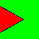
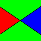
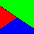
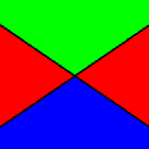
Figure 3: Top row ((E3) [a]): In the left-most panel, both particles die; they survive in the panel on the right and create a new polygon coloured blue. Bottom row ((eE3) [b]): In the left-most panel, one particles survives; both particles survive in the panel on the right and create a new polygon coloured red.

All particles evolve independently in time according to the following rules.

(E1) Between the critical moments listed below each particle moves freely with constant velocity.

(E2) When a particle hits the boundary $\partial D,$ it dies.

(E3) In case of a collision of two particles, that is, equal spatial coordinates $y$ at some time $t$ with $(t,y)=n(l_{i},l_{j})\in D$, distinguish the following cases.

a

If the colours above and below $(t,y)$ are identical, say $i$, with probability $\alpha_{V}$ both particles die. With probability $\alpha_{X}$ both particles survive to create a new polygon whose colour is chosen uniformly from those not equal to $i$ (cf. Figure 3).

b

If the colours above and below $(t,y)$ are different, say $i$ and $j$, with probability $\alpha_{T}$, each of the two particles survives while the other dies. With probability $(k-2)\alpha_{X}/(k-1)=1-2\alpha_{T}$, both particles survive to create a new polygon whose colour is chosen uniformly from those not equal to either $i$ or $j$ (cf. Figure 3).

Recall that a collision prevents a birth from happening at the node.

(E4) Whenever a particle moving in time-space along $l_{i}\in{\cal T}$ reaches a node $n(l_{i},l_{j}),$ it changes its velocity so as to move along $l_{j}$ with probability $\alpha_{V}\pi_{l_{j}}/(k-1)$, it splits into two particles moving along $l_{i}$ and $l_{j}$ with probability $(k-2)\alpha_{T}\pi_{l_{j}}/(k-1)$ and keeps moving along $l_{i}$ otherwise (with probability $1-\epsilon\pi_{l_{j}}$). In case of a split, a new polygon is created whose colour is chosen uniformly from the $k-2$ possibilities. See Figure 4.

The dynamics described above define a random coloured polygonal configuration $\hat{\cal{D}}_{D}$. The key observation is that its distribution is identical to that of $\hat{\cal{A}}_{\Phi_{D}}$.

Theorem 2.

The random elements $\hat{\cal{A}}_{\Phi_{D}}$ and $\hat{\cal{D}}_{D}$ coincide in distribution.

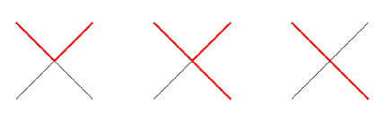
Figure 4: (E4): Velocity update (left), split (middle) and continuation (right) of a trajectory outlined in red.

Proof: In order to calculate the probability that some $\hat{\gamma}\in\hat{\Gamma}_{D}({\cal T})$ is generated by the particle dynamics E1–E4, observe that

• each edge $e\in E(\gamma)$ whose initial (lower time coordinate) vertex lies on $\partial D$ yields a factor ${\pi_{l[e]}}/(1+\pi_{l[e]})$ (boundary birth site) times $\prod_{l\in{\cal T},\;l\nsim e}(1-\epsilon\pi_{l})$ (no velocity/split updates along $e$) times $1/(k-1)$ for the colour;

• the two edges $e_{1},e_{2}\in E(\gamma)$ emanating from a common interior birth site $n(l_{1},l_{2})$ yield a factor $\alpha_{V}\pi_{l_{1}}\pi_{l_{2}}/(k-1)$ (the birth probability) times $\prod_{i=1}^{2}\prod_{l\in{\cal T},\;l\nsim e_{i}}(1-\epsilon\pi_{l})$ (no velocity/split updates along $e_{i}$) times $1/(k-1)$ for the colour;

• each edge $e\in E(\gamma)$ arising due to a velocity update yields a factor $\alpha_{V}\pi_{l[e]}/(k-1)$ (velocity update probability) times $\prod_{l\in{\cal T},\;l\nsim e}(1-\epsilon\pi_{l})$ (no velocity/split updates along $e$);

• the two edges $e_{1},e_{2}\in E(\gamma)$ arising from a split at node $n(l_{1},l_{2})$ where $e_{1}$ is a continuation and $e_{2}$ a new direction yield a factor $(k-2)\alpha_{T}\pi_{l_{2}}/(k-1)$ (the split probability) times $\prod_{i=1}^{2}\prod_{l\in{\cal T},\;l\nsim e_{i}}(1-\epsilon\pi_{l})$ (no velocity/split updates along $e_{i}$) times $1/(k-2)$ for the colour;

• the two edges $e_{1},e_{2}\in E(\gamma)$ arising due to an X-collision contribute a factor $\alpha_{X}/(k-1)$ times $\prod_{i=1}^{2}\prod_{l\in{\cal T},\;l\nsim e_{i}}(1-\epsilon\pi_{l})$ (no velocity/split updates along $e_{i}$);

• each edge $e$ emanating from a T-collision contributes a factor $\alpha_{T}$ times $\prod_{l\in{\cal T},\;l\nsim e}(1-\epsilon\pi_{l})$ (no velocity/split updates along $e$);

• each collision of V-type contributes a factor $\alpha_{V}$;

• the initial colour choice contributes a factor $1/k$;

• the absence of birth sites in nodes $n(l_{1},l_{2})\in D$ that do not belong to $\gamma$ yields the factor $\prod_{n(l_{1},l_{2})\in D\setminus\gamma}(1-\alpha_{V}\pi_{l_{1}}\pi_{l_{2}}/(k-1))$ ;

• the absence of boundary birth sites at those entry points into $D$ of lines of ${\cal T}$ which do not give rise to an edge of $\gamma$ yields the factor $\prod_{l\in{\cal T},\;l\cap D\neq\emptyset,\;{\rm{in}}(l,D)\not\in\gamma}(1+\pi_{l})^{-1}.$

Collecting all factors implies that the probability of $\hat{\gamma}$ is

$$\left(\prod_{e\in E(\gamma)}\prod_{l\in{\cal T},\;l\nsim e}(1-\epsilon\pi_{l})\right)\left(\prod_{n(l_{1},l_{2})\in D\setminus\gamma}\left(1-\frac{\alpha_{V}}{k-1}\pi_{l_{1}}\pi_{l_{2}}\right)\right)\times\left(\prod_{l\in{\cal T},\;l\cap D\neq\emptyset}\frac{1}{1+\pi_{l}}\right)$$

times

$$\frac{1}{k}\,\alpha_{V}^{N_{V}}\,\left(\alpha_{T}(k-1)\right)^{N_{T}}\,\left(\alpha_{X}(k-1)\right)^{N_{X}}\prod_{e\in E^{*}(\gamma)}\pi_{l[e]}\times\prod_{e\in E(\gamma)}\frac{1}{k-1},$$

which completes the proof. $\square$

As an immediate consequence of the proof of Theorem 2, we obtain an explicit and simple expression for the partition function of consistent polygonal fields.

Corollary 1.

The partition function (2) is given by

$$k\prod_{l\in{\cal T},\;l\cap D\neq\emptyset}(1+\pi_{l})\prod_{n(l_{1},l_{2})\in D}\left(1-\frac{\alpha_{V}}{k-1}\pi_{l_{1}}\pi_{l_{2}}\right)^{-1}$$

Having established a proper dynamic representation, Theorem 1 follows from Theorem 2 in complete analogy with the proof of [2, Thm. 5.1] as in [23, Thm. 1]. A discrete analogue of the Poisson line transect property [2, Thm. 5.1.c] holds as well. Indeed, combining consistency with the boundary birth mechanism of the dynamical representation, we obtain the following.

Corollary 2.

Let $l$ be a straight line that contains no nodes of ${\cal T}$. Then, the intersection points and intersection directions of $l$ with the edges of the polygonal field $\hat{\cal A}_{\Phi}$ coincide in distribution with the intersection points and directions of $l$ with the line field $\Lambda_{\cal T}$ defined to be the random sub-collection of ${\cal T}$ where each straight line $l^{*}\in{\cal T}$ is chosen to belong to $\Lambda_{\cal T}$ with probability ${\pi_{l^{*}}}/(1+\pi_{l^{*}})$ and rejected otherwise, and all these choices are made independently.

To conclude this section, we turn to Markov properties that are direct consequences of the dynamic representation.

A spatial Markov property reminiscent of that enjoyed by the Arak–Clifford–Surgailis model in the continuum is the following. For a piece wise smooth simple closed curve $\theta\subset{\mathbb{R}}^{2}$ containing no nodes of ${\cal T}$, the conditional distribution of $\hat{\cal A}_{\Phi}$ in the interior of $\theta$ depends on the configuration exterior to $\theta$ only through the intersections of $\theta$ with the edges of the polygonal field and through the colouring of the field along $\theta.$

To relate our model to Gibbs fields commonly used in image analysis, assume for the remainder of this section that ${\cal{T}}$ forms a regular lattice and $D$ is an $m\times n$ rectangle. In this case, $D$ is divided by ${\cal{T}}$ in square cells, known as pixels. There is a one-to-one correspondence between a coloured polygonal configuration $\hat{\gamma}$ and the array of pixel colours. Indeed, the colour of a pixel is that of the face of $\hat{\gamma}$ that it falls in, and, reversely, the edges of $\gamma$ are composed of the segments between pixels of different colours. In this dual framework, we obtain the following local Markov factorisation.

Corollary 3.

Let $D$ be an $m\times n$ array and let ${\cal{T}}=\{l_{1},\dots,l_{m+n-2}\}$ be the corresponding regular linear tessellation with the indices chosen in such a way that for $i=1,\dots,n-1$, $l_{i}$ is the horizontal line between the $i$-th and $(i+1)$-st row and for $i=1,\dots,m-1$, $l_{n+i-1}$ is the vertical line between the $i$-th and $(i+1)$-st column. Then the random element $\hat{A}_{\Phi_{D}}$ is the dual of a random vector $X=(X_{1},\dots,X_{mn})$ of pixel values indexed in column major order with a joint probability mass function ${\mathbb{P}}(\hat{\gamma})={\mathbb{P}}(X_{1}=x_{1};\cdots;X_{mn}=x_{mn})$ that factorises as

$${\mathbb{P}}(X_{1}=x_{1})\prod_{i=2}^{n}{\mathbb{P}}(X_{i}=x_{i}\mid X_{i-1}=x_{i-1})\prod_{i=1}^{m-1}{\mathbb{P}}(X_{in+1}=x_{in+1}\mid X_{(i-1)n+1}=x_{(i-1)n+1})$$

$$\times\prod_{i=1}^{m-1}\prod_{j=2}^{n}{\mathbb{P}}(X_{in+j}=x_{in+j}\mid X_{(i-1)n+j-1}=x_{(i-1)n+j-1};$$

$$\quad\quad\quad\quad X_{(i-1)n+j}=x_{(i-1)n+j};X_{in+j-1}=x_{in+j-1})$$

for $x_{i}\in\{1,\dots,k\}$, $i=1,\dots,mn$.

Proof: Choose the time direction in the dynamic representation in such a way that the chronological order of the nodes coincides with the column major order and recall that the conditional behaviour at a node depends only on the colours and trajectories immediately to its ‘left’, i.e. immediately prior to it in time. For the first pixel, ${\mathbb{P}}(X_{1}=x_{1})$ is the probability that the initial colour is $x_{1}$, which is $1/k$ as this colour is chosen uniformly from the set $\{1,\dots,k\}$. Next, the probabilities of the pixel values in the first column are derived from the boundary birth mechanism. Thus, for $x_{i},x_{i-1}\in\{1,\dots,k\}$ and $i=2,\dots,n$,

$${\mathbb{P}}(X_{i}=x_{i}\mid X_{i-1}=x_{i-1})=\left\{\begin{array}[]{ll}\frac{1}{k-1}\,\frac{\pi_{l_{i-1}}}{1+\pi_{l_{i-1}}}&\mbox{ if }x_{i}\neq x_{i-1};\\ \frac{1}{1+\pi_{l_{i-1}}}&\mbox{ if }x_{i}=x_{i-1}.\end{array}\right.$$

Similarly, for $x_{in+1},x_{(i-1)n+1}\in\{1,\dots,k\}$ and $i=1,\dots,m-1$,

$${\mathbb{P}}(X_{in+1}=x_{in+1}\mid X_{(i-1)n+1}=x_{(i-1)n+1})=\left\{\begin{array}[]{ll}\frac{1}{k-1}\,\frac{\pi_{l_{i+n-1}}}{1+\pi_{l_{n+i-1}}}&\mbox{ if }x_{in+1}\neq x_{(i-1)n+1};\\ \frac{1}{1+\pi_{l_{n+i-1}}}&\mbox{ if }x_{in+1}=x_{(i-1)n+1}.\end{array}\right.$$

Use the shorthand notation ${\mathbb{P}}_{ij}(x\mid u,v,w)$ for

$${\mathbb{P}}(X_{in+j}=x_{in+j}\mid X_{(i-1)n+j-1}=u;X_{(i-1)n+j}=v;X_{in+j-1}=w).$$

Then, for $u\neq v\neq w\neq u$,

$${\mathbb{P}}_{ij}(x\mid u,v,v)=\left\{\begin{array}[]{ll}\alpha_{V}&\mbox{ if }x=v\\ \alpha_{X}/(k-1)&\mbox{ if }x\neq v\end{array}\right.$$

by (E3a), and

$${\mathbb{P}}_{ij}(x\mid u,v,w)=\left\{\begin{array}[]{ll}\alpha_{T}&\mbox{ if }x\in\{v,w\}\\ \alpha_{X}/(k-1)&\mbox{ if }x\not\in\{v,w\}\end{array}\right.$$

by (E3b) regardless of $i,j$. Furthermore, the interior birth mechanism implies that

$${\mathbb{P}}_{ij}(x\mid u,u,u)=\left\{\begin{array}[]{ll}\alpha_{V}\pi_{l_{j-1}}\pi_{l_{n+i-1}}/(k-1)^{2}&\mbox{ if }x\neq u\\ 1-\alpha_{V}\pi_{l_{j-1}}\pi_{l_{n+i-1}}/(k-1)&\mbox{ if }x=u\end{array}\right.$$

and finally (E4) determines the probabilities

$${\mathbb{P}}_{ij}(x\mid u,u,v)=\left\{\begin{array}[]{ll}1-\epsilon\pi_{l_{j-1}}&\mbox{ if }x=v\\ \alpha_{V}\pi_{l_{j-1}}/(k-1)&\mbox{ if }x=u\\ \alpha_{T}\pi_{l_{j-1}}/(k-1)&\mbox{ if }x\not\in\{u,v\}\end{array}\right.$$

and

$${\mathbb{P}}_{ij}(x\mid u,v,u)=\left\{\begin{array}[]{ll}1-\epsilon\pi_{l_{n+i-1}}&\mbox{ if }x=v;\\ \alpha_{V}\pi_{l_{n+i-1}}/(k-1)&\mbox{ if }x=u;\\ \alpha_{T}\pi_{l_{n+i-1}}/(k-1)&\mbox{ if }x\not\in\{u,v\}.\end{array}\right.$$

Collecting all terms completes the proof. $\square$

Models for which the above factorisation holds have been dubbed mutually compatible Gibbs random fields by Goutsias [9]. In particular, the interior birth mechanism, as well as the collisions and path propagation described in the dynamical representation’s (E3)–(E4) correspond to the local transfer function in [9], see also[5].

Note that we have chosen the time direction so as to conform to column major order. A fortiori, such models are Markov random fields with the second order neighbourhood structure in which horizontally, vertically, and diagonally adjacent pixels are neighbours. A similar factorisation holds for any choice of the time axis. Moreover, there is no need for $D$ to be a rectangle. Indeed, because of the assumptions on ${\cal{T}}$, every interior node is hit by exactly two segments that are adjacent to three, not necessarily rectangular, pixels. See Figure 6 for an example. The notation, however, becomes more cumbersome. For this reason, we prefer to use the graph-theoretical formulation with its neater formulae.

4 Birth and death dynamics

In this section, we use the dynamic representation of Section 3 to propose dynamics that are reversible and leave the law of $\hat{\cal{A}}_{\Phi_{D}}$ invariant. These dynamics will serve as stepping stone for building Metropolis–Hastings dynamics for the general polygonal field models (1). For the two-colour case, algorithms inspired by dynamic representations can be found in [11, 20, 23, 17]. In that case, however, it is sufficient to focus on colour blind polygonal configurations as the colouring is completely determined by the colour at a single point. For $k>2$, this is no longer the case and we have to explicitly incorporate colours in our dynamics. Moreover, particles do not necessarily die upon collision and the disagreement loop principle of Schreiber [20] no longer applies.

The basic continuous time dynamics we propose consist of adding and deleting particle birth sites. In order to fully explore the state space, recolouring will also be necessary, at some fixed rate $\tau>0$. We work with a constant death rate $1$. The birth rate at a boundary entry point ${\rm{in}}(l,D)$ and a vacant internal node $n(l_{1},l_{2})$ are set to $\pi_{l}$ and $\alpha_{V}\pi_{l_{1}}\pi_{l_{2}}/(k-1-\alpha_{V}\pi_{l_{1}}\pi_{l_{2}})$ to satisfy the detailed balance equations

$$\frac{\pi_{l}}{1+\pi_{l}}\times 1=\left(1-\frac{\pi_{l}}{1+\pi_{l}}\right)\times\mbox{birth rate}({\rm{in}}(l,D))$$

respectively

$$\frac{\alpha_{V}}{k-1}\pi_{l_{1}}\pi_{l_{2}}\times 1=\left(1-\frac{\alpha_{V}}{k-1}\pi_{l_{1}}\pi_{l_{2}}\right)\times\mbox{birth rate}(n(l_{1},l_{2})).$$

Recall that if $n(l_{1},l_{2})$ is hit by some previously born particle, the birth is discarded. For computational convenience, we shall keep track of the discarded births during the dynamics.

In case of a birth update, the particle(s) emitted by the birth site are given trajectories in accordance with E4. Upon collisions, E3 is invoked. Whenever possible, existing trajectories are re-used. A dual reasoning is applied to deaths.

To make the above ideas precise, suppose that the current state is $\hat{\gamma}$, understood here to include the knowledge of all discarded birth sites, which we modify by adding or deleting a (discarded) birth site to obtain $\hat{\gamma}^{\prime}$. We shall use the following segment classification:

plus

the segment does not lie on any edge of $\gamma$ but it does lie on some edge of $\gamma^{\prime}$;

minus

the segment lies on some edge of $\gamma$ but it does not lie on any edge of $\gamma^{\prime}$;

changed

the segment lies on some common edge of $\gamma$ and $\gamma^{\prime}$ but the colour of at least one of its adjacent polygonal faces has changed, or the segment lies in the interior of faces of $\hat{\gamma}$ and $\hat{\gamma}^{\prime}$ having different colours.

The dynamics are now as follows. In case of a birth at node $n(l_{1},l_{2})$ with coordinates $(t,y)$, two plus segments arise along $l_{1}$ and $l_{2}$ forward in time. In case of a boundary birth, a single plus segment is generated. Similarly, in case of a death, one or two minus segments arise. We order the nodes with first coordinate larger than $t$ in chronological order and update them one at a time until some further time $t^{\prime}>t$ for which the intersections of $\hat{\gamma}$ and $\hat{\gamma}^{\prime}$ with the vertical line specified by first coordinate $t^{\prime}$ are identical.

At each node, we first check whether the node is hit either by some segment marked ‘plus’ or ‘minus’, or by some ‘changed’ segment of $\gamma$. When using the word ‘hit’ we shall always mean that the tail of the segment has a smaller time coordinate than the node at its head. We shall use the phrase ‘emanating segments’ for those segments whose tail is at the node and whose head has a larger time coordinate than the node. If no such segment exists, we need to check whether the node is a non-discarded birth site. If it is, due to e.g. nesting, the colour just prior to the birth site may be different in $\hat{\gamma}$ and $\hat{\gamma}^{\prime}$. In this case, a new colour is chosen for the region to the right of the node from those not equal to the colour just prior to the node. Otherwise, the status quo is propagated.

If the node is hit by two marked segments (‘plus’, ‘minus’ or ‘changed’ and belonging to $\gamma$), or by one such segment and one that is an unchanged common edge of $\gamma$ and $\gamma^{\prime}$ (which we label ‘old’) a collision update is made as outlined in Table 1.

minus/minus	label emanating segments;
at vacant node
minus/minus	implement birth by choosing new colour from those
at discarded birth site	not equal to that prior to the discarded birth site;
	label emanating segments;
minus/old	invoke E4;
minus/plus	label emanating segments;
minus/changed
plus/old	invoke E3;
plus/changed	label emanating segments;
old/changed
plus/plus at
vacant node
plus/plus	discard the birth;
at birth site	invoke E3 and label emanating segments;
changed/changed	check whether the colours above and below the face
	bounded by the two hitting segments agree in $\hat{\gamma}$ and $\hat{\gamma}^{\prime}$;
	if so, do nothing;
	otherwise invoke E3 and label emanating segments.

Table 1: Collision updates.

In the remaining case that the node is hit by a single segment marked either ‘plus’ or ‘minus’ or by a segment of $\gamma$ labelled ‘changed’, the path is updated as outlined in Table 2.

plus path	discard the birth;
at birth site	invoke E4;
	label emanating segments;
plus path	invoke E4;
at vacant site	label emanating segments;
minus path	implement birth by choosing new colour from those
at discarded birth site	not equal to that prior to the discarded birth site;
	label emanating segments;
minus path	label emanating segments;
at vacant site
changed path	in case the path splits, choose a new colour
	from those not equal to the colours above and below the path;
	label emanating segments.

Table 2: Path updates.

An illustration is given in Figure 5. The current node $n$ to be updated is in the middle of the panels. In $\hat{\gamma}$, the node is a birth site: no segments hit $n$ and there are two emanating segments. In the new polygonal configuration $\hat{\gamma}^{\prime}$, the node is hit by a segment separating the green from the blue face which is therefore labelled ‘plus’. According to Table 2, in $\hat{\gamma}^{\prime}$, the birth gets discarded and we invoke E4, say resulting in the decision to split. Hence, we must also choose a colour other than green or blue for the region to the right, that is, forwards in time, for example red. The labels of the two emanating segments are ‘changed’ for the one separating the blue and red faces, and ‘old’ for the one forming the boundary between the red and green faces.

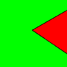
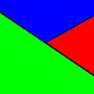
Figure 5: Left: $\hat{\gamma}$. Right: $\hat{\gamma}^{\prime}$.

For recolouring, classic local colour switches are used, as detailed in for example [29]. As for the two-colour case in [23], we obtain the following result.

Theorem 3.

The distribution of the consistent polygonal field $\hat{\cal{A}}_{\Phi_{D}}$ is the unique invariant probability distribution of the birth-death-recolour dynamics described above upon ignoring discarded birth attempts, to which they converge in total variation from any initial state $\hat{\gamma}\in\hat{\Gamma}_{D}({\cal{T}})$ for which ${\mathbb{P}}(\hat{\cal{A}}_{\Phi_{D}}=\hat{\gamma})>0$.

Proof: The case $k=2$ was considered in [23]. Hence assume $k>2$. The total transition rate is bounded from above by a positive constant. Indeed, for each internal birth site $n(l_{1},l_{2})$, the rate

$$\frac{\alpha_{V}\pi_{l_{1}}\pi_{l_{2}}/(k-1)}{1-\alpha_{V}\pi_{l_{1}}\pi_{l_{2}}/(k-1)}\leq\frac{1/(k-1)}{1-1/(k-1)}=\frac{1}{k-2}\leq 1.$$

The death rate for a (discarded) birth at $n(l_{1},l_{2})$ is equal to $1$. Similarly, the birth rate $\pi_{l}$ at entry points $\rm{in}(l,D)=\pi_{l}\leq 1$ and the death rate is again equal to $1$. Therefore, an upper bound is the sum of $\tau$, the number of nodes and the number of lines hitting $D$. Thus, our dynamics can be algorithmically generated by a Poisson clock of constant rate, and an embedded Markov transition matrix that governs the transitions. This transition matrix restricted to admissible coloured polygonal configurations with positive probability under the putative invariant probability distribution is irreducible, since any state can be reached from any other state by successively removing all birth attempts, choosing an appropriate initial colour and then building the target state by successively adding particles. Hence the dynamics constitute a finite state space irreducible Markov process and there exists a unique invariant probability distribution. See for example Theorem 20.1 in [13]. The same theorem also yields the converge in total variation. The invariance of the distribution including discarded birth attempts follows from the invariance of the Bernoulli birth site probabilities under the dynamics, the fact that the trajectories preserve E1–E4 by design, and the well-known invariance of the local colour switches [29, Section 10.2]. Summing over any discarded birth attempts completes the proof. $\square$

In fact, the dynamics are reversible. Consider for example the collision of a positive path with a birth site as in Figure 5. In this example, the transition rate is multiplied by $(k-2)\alpha_{T}\pi_{l_{j}}/(k-1)$ for the split and $1/(k-2)$ for the colour, amounting to $\alpha_{T}\pi_{l_{j}}/(k-1)$ whereas the probability of $\hat{\gamma}$ including the knowledge of discarded births gains a factor $(k-1)\alpha_{T}\pi_{l_{j}}/(k-1)=\alpha_{T}\pi_{l_{j}}$ (the first term $k-1$ to compensate for the choice of colour in $\hat{\gamma}$, the second for the split and colour in $\hat{\gamma}^{\prime}$). The reverse collision of a minus path with a discarded birth site yields a factor $1/(k-1)$ for the rate. Thus, this type of collision is reversible. Similar calculations can be made for the other types of collision and are left to the reader.

For general polygonal field models (1) with a Hamiltonian that is the sum of (3) and some other term ${\cal{H}}_{D}$, we propose a Metropolis–Hastings algorithm. The algorithm has the same birth, death and recolour rates as the dynamics presented in Section 4. The difference is that a new state $\hat{\gamma}^{\prime}$ is accepted with probability

$$\min\left(1,\exp\left[{\cal{H}}_{D}(\hat{\gamma})-{\cal{H}}_{D}(\hat{\gamma}^{\prime})\right]\right),$$ (4)

whereas the old state is kept with the complementary probability. An example of ${\cal{H}}_{D}$ will be presented in Section 5.

Theorem 4.

Let ${\cal{H}}_{D}:\hat{\Gamma}_{D}({\cal T})\mapsto{\mathbb{R}}$ be finite. Then the distribution of the polygonal field $\hat{\cal{A}}_{\Phi_{D}+{\cal{H}}_{D}}$ is the unique invariant probability distribution of the Metropolis–Hastings dynamics. Moreover, these dynamics converge in total variation to $\hat{\cal{A}}_{\Phi_{D}+{\cal{H}}_{D}}$ from any initial state $\hat{\gamma}\in\hat{\Gamma}_{D}({\cal{T}})$ for which ${\mathbb{P}}(\hat{\cal{A}}_{\Phi_{D}}=\hat{\gamma})>0$.

Proof: By the assumption on the Hamiltonian and arguments analogous to those in the proof of Theorem 3, the embedded Markov transition matrix that governs the transitions is irreducible. Hence the dynamics constitute a finite state space irreducible Markov process and there exists a unique invariant probability distribution, cf. Theorem 20.1 in [13], to which they converge in total variation. By Theorem 3, the birth-death-recolour dynamics leave the distribution of $\hat{\cal{A}}_{\Phi_{D}}$ invariant. The modification by the acceptance probabilities (4) yields that the target distribution $\hat{\cal{A}}_{\Phi_{D}+{\cal{H}}}$ is left invariant by the Metropolis–Hastings dynamics. $\square$

5 Application to linear network extraction

The goal of this section is to apply the model presented in Section 2 to the extraction of a network of tracks in between crop fields from image data. The left-most panel in Figure 6, obtained from the collection of publicly released SAR (Synthetic Aperture Radar) images at the NASA/JPL web site http://southport.jpl.nasa.gov shows an agricultural region in Ukraine. A pattern of fields separated by tracks is visible, broken by some hamlets. The image was previously analysed by Stoica et al. [25] by means of a Markov line segment process.

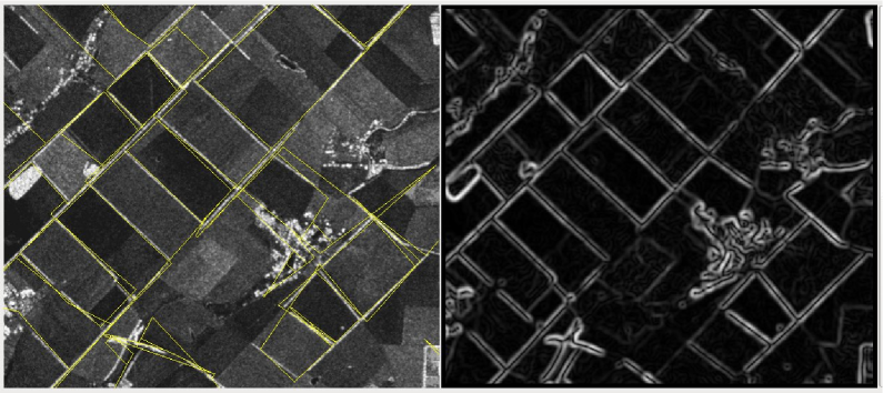
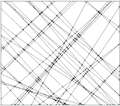
Figure 6: Polygonal configuration (in yellow) overlaid on a SAR image of fields in rural Ukraine (top left panel), the corresponding edge map (top right panel) and a regular linear tessellation extracted from the Hough accumulation array (bottom row).

Note that the tracks that run between adjacent fields show up in the image as whitish lines against the darker fields. Thus, a track is associated with a high image gradient. To find a suitable family ${\cal{T}}$ of straight lines, we therefore begin by computing the gradient of the data image after convolution with a radially symmetric Gaussian kernel with standard deviation $\sigma=3$ to suppress noise. The right-most panel in Figure 6 shows the gradient length thus obtained. We then compute the Hough transform [8, 10] in an $80\times 80$ accumulation array and select the $8$ lines corresponding to the bins with the largest number of accumulated votes. This collection is augmented by lines parametrised by the largest local extrema in the accumulation array to yield the $42$ lines shown in the bottom panel of Figure 6. The resulting set is finite and contains no three lines that intersect in a common point, in other words, it is a regular linear tessellation. Regarding the choice of $\alpha_{V}$, a comparison of the data with the simulations shown in Figure 2 suggests $\alpha_{V}=1/2$. Since the lines are selected on the basis of a high gradient value, there seems to be no particular reason to favour one line over another, so we may set the line activity to a constant value.

To quantify how well a polygonal configuration fits the data, recall that an edge should be present when there is a large gradient, and absent when the gradient is small. This desirable property is captured by the Hamiltonian

$${\cal{H}}_{D}(\hat{\gamma})=-\beta\sum_{e\in E(\gamma)}\left[f(e)-c(e)\right],$$ (5)

where $f(e)$ is the integrated absolute gradient flux along edge $e$, $c(e)$ a threshold to discourage spurious edges, and $\beta>0$. We take $c(e)$ proportional to the number of segments along the edge with proportionality constant $c>0$. For this choice, (5), being a sum of segment contributions, is local in nature, which is convenient from a computational perspective.

To find an optimal polygonal configuration, we use simulated annealing applied to the Metropolis–Hastings algorithm of Section 3 for $\hat{\cal{A}}_{\Phi_{D}+{\cal{H}}_{D}}$ with $\Phi_{D}$ given by (3) and ${\cal{H}}_{D}$ defined by (5) and recolour rate $100$. Starting at temperature $1/\beta=10$, the inverse temperature parameter $\beta$ is slowly increased to $100$ according to a geometric cooling schedule. The result for $c=2$, line activity $1/2$ and $k=4$ is shown in Figure 6. There are no false negatives; a few false positives occur near the hamlets and are connected to the track network. The precision of the line placement is clearly linked to the precision of the underlying regular linear tessellation.

6 Summary and discussion

In this paper, a new class of consistent random fields was introduced whose realisations are coloured mosaics with not necessarily convex polygonal tiles. The vertices of the polygonal tiles may have degrees two, three or four. The construction, inspired by the Arak–Clifford–Surgailis polygonal Markov fields in the continuum [2, 3, 4], extends our previous construction [23] of consistent polygonal random fields with tile vertices of degree two only. The latter case is substantially simpler due to the fact that interactions are restricted to a hard core constraint only, and, moreover, for a given realisation, there are only two equally likely admissible colourings. We developed a dynamic representation for consistent multi-colour polygonal fields, which was used to prove the basic properties of the model including consistency and an explicit expression for the partition function. Local and spatial Markov properties were also considered. The dynamic representation provided the foundation on which to build Metropolis–Hastings style samplers for Gibbsian modifications of these fields. Finally, we applied the model to the detection of linear networks in rural scenes. A modification of our models would consist in ascribing activity parameters to segments rather than lines, cf. [17]. A disadvantage seems to be that the dynamic representation would depend on the direction of time, in other words, the model would be anisotropic.

To conclude, we should stress that, although the model was inspired by those of Arak et al.  there are striking differences inherent to the discrete set-up. Notably, in the continuum collinear edges are not allowed, in the discrete set-up they are. Indeed, if one were to forbid collinear edges, this would lead to a forbidden line whose influence would be felt at arbitrarily large distance from its single edge, hence ruling out any meaningful Markovianity. This is not true in the continuum as the dynamic representation there ensures that collinear edges occur with probability zero. As a consequence, our consistent random fields are not Arak–Surgailis fields conditional on having their edges along the lines of ${\cal{T}}$. More fruitfully, our models provide a graph-theoretical interpretation of mutually compatible Gibbs random fields that inspires novel simulation algorithms as an alternative to the usual local tile updating schemes [29].

References

- [1] Arak, T. (1982). On Markovian random fields with finite number of values. 4th USSR-Japan symposium on probability theory and mathematical statistics, Abstracts of Communications, Tbilisi.
- [2] Arak, T., and Surgailis, D. (1989). Markov fields with polygonal realisations. Probab. Theory Related Fields 80, 543–579.
- [3] Arak, T., and Surgailis, D. (1991). Consistent polygonal fields. Probab. Theory Related Fields 89, 319–346.
- [4] Arak, T., Clifford, P., and Surgailis, D. (1993). Point-based polygonal models for random graphs. Adv. in Appl. Probab. 25, 348–372.
- [5] Champagnat, F., Idier, J., and Goussard, Y. (1998). Stationary Markov random fields on a finite rectangular lattice. IEEE Trans. Inform. Theory 44, 2901–2916.
- [6] Clifford, P., and Middleton, R.D. (1989). Reconstruction of polygonal images. J. Appl. Stat. 16, 409–422.
-
[7]
Clifford, P., and Nicholls, G. (1994).
A Metropolis sampler for polygonal image reconstruction.
Available at:
http://www.stats.ox.ac.uk/clifford/papers/met_poly.html - [8] Duda, R.O., and Hart, P.E. (1972). Use of the Hough transformation to detect lines and curves in pictures. Commun. ACM 15, 11–15.
- [9] Goutsias, J.K. (1989). Mutually compatible Gibbs random fields. IEEE Trans. Inform. Theory 35, 1233–1249.
- [10] Hough, P.V.C. (1962). Method and means for recognizing complex patterns. US Patent 3069654.
- [11] Kluszczyński, R., Lieshout, M.N.M. van, and Schreiber, T. (2005). An algorithm for binary image segmentation using polygonal Markov fields. In: F. Roli and S. Vitulano (Eds.), Image Analysis and Processing, Proceedings of the 13th International Conference on Image Analysis and Processing. Lecture Notes in Comput. Sci. 3615, 383–390.
- [12] Kluszczyński, R., Lieshout, M.N.M. van, and Schreiber, T. (2007). Image segmentation by polygonal Markov fields. Ann. Inst. Stat. Math. 59, 465–486.
- [13] Levin, D.A., Peres, Y., and Wilmer, E.L. (2008). Markov chains and mixing times. American Mathematical Society, Providence.
- [14] Lieshout, M.N.M. van, and Schreiber, T. (2007). Perfect simulation for length-interacting polygonal Markov fields in the plane. Scand. J. Statist. 34, 615–625.
- [15] Lieshout, M.N.M. van (2012). An introduction to planar random tessellation models. Spatial Statistics 1, 40–49.
- [16] Mackisack, M.S., and Miles, R.E. (2002). A large class of random tessellations with classical Poisson polygon distributions. Forma 17, 1–17.
- [17] Matuszak, M., and Schreiber, T. (2012). Locally specified polygonal Markov fields for image segmentation. In: L. Florack, R. Duits, G. Jongbloed, M.-C. van Lieshout and L. Davies (Eds.), Mathematical Methods for Signal and Image Analysis and Representation. Computational Imaging and Vision 41, 261–274.
- [18] Nicholls, G.K. (2001). Spontaneous magnetization in the plane. J. Stat. Phys. 102, 1229–1251.
- [19] Paskin, M.A., and Thrun, S. (2005). Robotic mapping with polygonal random fields. In: Proceedings in Artificial Intelligence UAI-05.
- [20] Schreiber, T. (2005). Random dynamics and thermodynamic limits for polygonal Markov fields in the plane. Adv. in Appl. Probab. 37, 884–907.
- [21] Schreiber, T. (2006). Dobrushin–Kotecký–Shlosman theorem for polygonal Markov fields in the plane. J. Stat. Phys. 123, 631–684.
- [22] Schreiber, T. (2008). Non-homogeneous polygonal Markov fields in the plane: graphical representations and geometry of higher order correlations. J. Stat. Phys. 132, 669–705.
- [23] Schreiber, T., and Lieshout, M.N.M. van (2010). Disagreement loop and path creation/annihilation algorithms for binary planar Markov fields with applications to image segmentation. Scand. J. Statist. 37, 264–285.
- [24] Schreiber, T. (2010). Polygonal web representation for higher order correlation functions of consistent polygonal Markov fields in the plane. J. Stat. Phys. 140, 752–783.
- [25] Stoica, R.S., Descombes, X., Lieshout, M.N.M. van, and Zerubia, J. (2002). An application of marked point processes to the extraction of linear networks from images. In: J. Mateu and F. Montes (Eds.), Spatial Statistics: Case Studies, pp. 287–312. WIT Press, Southampton.
- [26] Surgailis, D. (1991). The thermodynamic limit of polygonal models. Acta Appl. Math. 22, 77–102.
- [27] Tha̋le, C. (2011). Arak–Clifford–Surgailis tessellations. Basic properties and variance of the total edge length. J. Stat. Phys. 144, 1329–1339.
- [28] Weiss, V., and Cowan, R. (2011). Topological relationships in spatial tessellations. Adv. in Appl. Probab. 43, 963–984.
- [29] Winkler, G. (2003). Image analysis, random fields and Markov chain Monte Carlo methods, A mathematical introduction, 2nd ed. Applications of Mathematics, Stochastic Modelling and Applied Probability 27. Springer-Verlag, Berlin.