Predicting the Fate of Binary Red Giants Using the Observed Sequence E Star Population: Binary Planetary Nebula Nuclei and Post-RGB Stars

Abstract

Sequence E variables are close binary red giants that show ellipsoidal light variations. They are likely the immediate precursors of planetary nebulae (PNe) with close binary central, stars as well as other binary post-AGB and binary post-RGB stars. We have made a Monte Carlo simulation to determine the fraction of red giant binaries that go through a common envelope (CE) event leading to the production of a close binary system or a merged star. The novel aspect of this simulation is that we use the observed frequency of sequence E binaries in the LMC to normalize our calculations. This normalization allows us to produce predictions that are relatively independent of model assumptions. In our standard model, and assuming that the relative numbers of PNe of various types are proportional to their birthrates, we find that in the LMC today the fraction of PNe with close binary central stars is 7–9%, the fraction of PNe with intermediate period binary central stars having separations capable of influencing the nebula shape (orbital periods less than 500 years) is 23–27%, the fraction of PNe containing wide binaries that are unable to influence the nebula shape (orbital period greater than 500 years) is 46–55%, the fraction of PNe derived from single stars is 3–19% and 5-6% of PNe are produced by previously merged stars. We also predict that the birthrate of post-RGB stars is $\sim$4% of the total PN birthrate, equivalent to $\sim$50% of the production rate of PNe with close binary central stars. These post-RGB stars most likely appear initially as luminous low-mass helium white dwarf binaries. The average lifetime of sequence E ellipsoidal variability with amplitude more than 0.02 magnitudes is predicted to be $\sim$0.95 Myr. We use our model and the observed number of red giant stars in the top one magnitude of the RGB in the LMC to predict the number of PNe in the LMC. We predict 548 PNe in good agreement with the 541$\pm$89 PNe observed by Reid & Parker (2006). Since most of these PNe come from single or non-interacting binary stars in our model, this means that most such stars produce PNe contrary to the “Binary Hypothesis” which suggests that binary interaction is required to produce a PN.

1 Introduction

In the LMC and SMC, red giant variables follow at least five Period-Luminosity relations, originally named sequences A to E (Wood et al., 1999). Sequence A, B and C are radial pulsation sequences and sequence D, which is parallel to sequences A, B and C but of longer period, is still of unknown physical origin (Wood, Olivier, & Kawaler, 2004; Nicholls et al., 2009; Nie, Zhang, & Jiang, 2010). Sequence E stars follow a loose Period-Luminosity relation between sequences C and D, but they extend to lower luminosities. Sequence E stars are widely accepted to be binaries (Wood et al., 1999; Soszyński et al., 2004). The orbital periods of the sequence E red giants are typically 100–600 days and the full light curve amplitudes are less than 0.6 mag in the MACHO red ($M_{R}$) band. They lie on the first giant branch in the case of low-mass stars, or the equivalent pre-core helium burning giant phase of intermediate mass stars (Wood et al., 1999). Some of the sequence E stars also extend to the AGB (Soszyński et al., 2004; Soszyński, 2007). As a whole, sequence E stars make up approximately 0.5–2% of the RGB and AGB stars in the Large Magellanic Cloud (LMC).

Sequence E variables show ellipsoidal light variations (Soszyński et al., 2004). In these systems, the primary star has evolved to the red giant phase and substantially filled its Roche lobe. Because the orbital separation of the system is similar to the size of the red giant, the red giant is distorted from spherical symmetry to an ellipsoid or pear-like shape by tidal interactions with its unseen companion. It is the orbital rotation of this shape that gives rise to the ellipsoidal light variations. About 7% of sequence E variables show eclipses in addition to the ellipsoidal light variations (Soszyński et al., 2004).

The first radial velocity curves of sequence E stars were presented in Nicholls, Wood, & Cioni (2010) and from their observations, the mean full velocity amplitude is about 43 km s^-1. This is consistent with the amplitudes expected for close red giant binaries with roughly solar-mass components. The velocity variation of the ellipsoidal variable is regular, dominated by its orbital motion. For every single cycle of the velocity variation there are two cycles of light variation, the latter being caused by the change in apparent surface area.

In past and ongoing radial velocity studies of sequence E stars in the LMC, we have obtained spectra for 110 systems. In none of these systems do we see the emission lines characteristic of symbiotic stars. This means that the companion is unlikely to be a white dwarf or neutron star. It is presumably a main-sequence star so that the red giant is usually the primary star in the binary system.

As the Roche lobe of the sequence E red variables is already substantially filled, further expansion of the red giant as it evolves is expected to soon cause Roche lobe overflow. The binary system will suffer a common envelope (CE) event (except in the rare case that the red giant has previously lost sufficient mass that mass transfer is stable). A CE event will lead to the ejection of the red giant envelope and the termination of RGB or AGB evolution. If the two stellar cores do not merge in the CE event, a luminous compact close binary system will be left. In the case of a CE event occurring on the RGB, the compact system will be a low mass white dwarf binary; while on the AGB, the remnant stellar core will be the central star of a planetary nebula (PN). If the two stellar cores do merge they should form a rapidly rotating red giant of the FK Comae class (Webbink, 1976; Bopp & Stencel, 1981; Bopp & Rucinski, 1981). The fraction of the rapidly rotating red giants is about 2% (Carlberg et al., 2011), although many of these stars may be tidally locked binaries rather than single stars.

The most common morphology of PNe is nonspherical and there are several theories attempting to explain the underlying mechanisms responsible for the shaping. Among all the mechanisms, the binary hypothesis is most favoured (Bond & Livio, 1990; Yungelson, Tutukov, & Livio, 1993; Soker, 1997; Bond, 2000; Zijlstra, 2007; De Marco, 2009) and it has been confirmed by observations in some cases. In fact, the shape of PNe with close binary central stars is definitely observed to be asymmetric. It has been suggested that binary interaction plays a major role in the formation and shaping of many (Bond & Livio, 1990; Iben & Livio, 1993), or even most PNe (Bond, 2000; De Marco, 2009).

At the present time, the actual fraction of PNe with close binary central stars is not clear. The short periods of the known central stars of binary PNe mean that these stars have been through a CE phase since the companion currently lies well within the radius of the precursor star when it was a red giant. It seems fairly clear that the brighter sequence E stars are indeed the immediate precursors of the known binary PNe central stars. At lower luminosities, the low mass white dwarf binaries, which are produced from RGB binaries (e.g. Paczynski, 1976; Webbink, 1984), should be descendants of sequence E stars. It is our aim to use the observed fraction of sequence E stars among all red giants to estimate the fraction of PNe with close binary central stars. We also use the sequence E fraction and the overall population of RGB stars in the LMC to estimate the birthrate and population of all PNe there, along with the birthrate of low mass white dwarf binaries.

In a study using MACHO light curves of stars in a central part of the LMC bar, Wood et al. (1999) found that $\sim$0.5% of the red giants in the top one magnitude of the RGB were detected as sequence E variables in the $M_{R}$ band. Similarly, Soszyński et al. (2004) and Soszyński (2007) using OGLE II data found that 1–2% of red giants were detected as sequence E variables. These numbers provide the calibrating input for the fractions of close binary PNe and low mass helium white dwarfs produced by CE events. Simultaneously, with this calibration, we can also estimate the fraction of red giants that are in wider binaries which reach the AGB tip without Roche lobe filling, and the fraction of PNe that are descended from single stars.

2 The Simulation Model

The prediction of the evolutionary fate of binary and single red giants is made by a Monte Carlo simulation. One million red giant binary systems are generated using orbital element distributions derived from observations of stars in the solar vicinity. The evolutionary fate of these binary systems is then examined. Single stars are added to the total stellar population in order to reproduce the observed fraction of sequence E stars on the red giant branch. Details of the standard simulation model are described in Section 2.1. Besides the standard model, we adjust the inputs to see how dependent the results are on the model assumptions. Results obtained by varying one or multiple parameters are described in Section 4. Since we will be utilizing the observed sequence E population in the LMC, our model uses inputs from LMC sources when available.

2.1 The standard model

2.1.1 Generating the binary system

1. The initial mass of the primary star
   Initially we require the red giant to be the primary star in the binary systems. The primary mass is drawn from the initial mass distribution $h(m,t)$ defined by

   $$dN=h(m,t)dmdt~{}~{},$$ (1)

   where $h(m,t)$ is the number of stars born per unit mass per unit time. To obtain $h(m,t)$, we consider the Initial Mass Function (IMF) as well as the star formation history. Let $g(m)$ be the IMF (assumed independent of time) and let $f(t)$ be the total star formation rate at time $t$, then $h(m,t)$ is expressed as:

   $$h(m,t)=g(m)\times f(t)~{}~{}.$$ (2)

   Here, $g(m)$ is assumed to follow the Salpeter (1955) power law: $g(m)=m^{-2.35}$. An observationally-based approximation to the LMC star formation history (Bertelli et al., 1992) has a star burst which starts $\sim$4 Gyrs ago and ceases $\sim$0.5 Gyrs ago, with the ratio of burst to quiescent star formation rate $R_{\rm burst}$ being 10. Thus, $f(t)$ is expressed as:

   $$f(t)=\left\{\begin{array}[]{cc}0~{},&t<0.5\\ R_{\rm burst}\times{b}~{},&0.5<t<4~{}~{},\\ b~{},&t>4\end{array}\right.$$

   where $R_{\rm burst}$=10, $b$ is a constant, and $t$ is in Gyrs from the present time. According to the evolutionary tracks of Girardi et al. (2000) appropriate for the LMC (Z=0.008), after converting the ages of red giants to initial masses, we have:

   $$f(t(m))=k(m)=\left\{\begin{array}[]{cc}0~{},&m>3.0\\ R_{\rm burst}\times{b}~{},&3.0>m>1.3~{}~{},\\ b~{},&m<1.3\end{array}\right.$$ (3)

   where $m$ is in solar masses.

   With the initial mass distribution, the cumulative probability distribution of the mass, $H(m)$, is expressed by:

   $$H(m)=\int_{m_{0}}^{m}{g(m)\times k(m)dm}~{}~{},$$ (4)

   where $m_{0}$ corresponds to the oldest stars currently on the giant branch.

   As we only consider red giant stars, the mass range should be that of RGB and AGB stars. The evolutionary tracks of Girardi et al. (2000) show that the minimum mass of low-mass stars in the LMC that are currently on the first giant branch is about $\rm{0.9~{}M_{\odot}}$. Stars with $m<\rm{0.9~{}M_{\odot}}$ have not yet evolved to the RGB since such stars have a main sequence lifetime longer than the time since the first stars formed. Hence, in Equation (4) we set $m_{0}$ to $\rm{0.9~{}M_{\odot}}$. The upper limiting mass for RGB stars which develop electron degenerate helium cores on the first ascent of giant branch, is about $\rm{1.85~{}M_{\odot}}$. Stars with mass larger than this do not reach the high luminosities of the observed sequence E stars in the LMC until they enter the early-AGB (EAGB). As the LMC star formation is assumed to cease 0.5 Gyrs ago, the maximum mass for AGB stars is $\rm{3.0~{}M_{\odot}}$. In the Monte Carlo simulation, we adjust ‘$b$’ so that $H(3.0)=1$, and draw the primary mass from the normalized $H(m)$.

2. The initial mass ratio
   We define $q=m_{2}/m_{1}$ as the mass ratio, where $m_{1}$ is the mass of the primary star and $m_{2}$ is the mass of the secondary star.

   The initial mass ratio is drawn from the distribution given in Duquennoy & Mayor (1991) who give orbital element distributions for binary stars in the solar vicinity. The mass ratio distribution follows a Gaussian-type relation, with a peak at 0.23. The reason we use the distribution from the solar vicinity (as well as the orbital period distribution described below) is that the mass ratio distribution is unknown observationally in the LMC.

   Given that we now know both masses in the binary system, we can decide which component is ‘currently’ being seen as the red giant. This is done by randomly assigning the primary or the secondary as the current red giant with probabilities that are proportional to the star formation rate at the time the system would have been born if the primary or secondary, respectively, was the current red giant. In the case where the secondary is the current red giant, the full evolution of the primary is followed before the evolution of the secondary is considered.

3. The orbital period
   The initial orbital period ($P$) is drawn from the distribution given in Duquennoy & Mayor (1991). The period distribution follows a Gaussian-type relation, with a peak of log$P$=4.8, in unit of days.

   Note that some binaries with long periods are too wide to influence the shape of PNe. Soker, Rappaport, & Harpaz (1998) suggest $P<$ 500–2000 years if a wide binary is to influence a PN shape. Mastrodemos & Morris (1999) similarly give a gravitational focusing fraction $\alpha_{foc}$ greater than 0.03 for a binary to produce a shell more distorted than “quasi-spherical”. If we apply this to low-mass stars with masses of $\sim$$1.5~{}\rm{M_{\odot}}$ and wind velocities of $\sim$10 km s^-1, we find $P<$ several hundred years is required. Based on the above, we adopt 500 years as the upper limiting period $P_{\rm max}$ for a wide binary to influence the shape of a PN. Hereinafter, we refer to binaries with $P>P_{\rm max}$ as ‘wide binaries’ and binaries with $P<P_{\rm max}$ but with periods large enough to avoid Roche lobe overflow on the RGB and AGB as ‘intermediate period’ binaries.

4. Eccentricity and stellar separation
   About 90% of the observed light curves of sequence E stars indicate zero or small eccentricity (Soszyński et al., 2004), so we assume zero eccentricity. Given the primary mass, mass ratio and orbital period, and assumed zero eccentricity, we can calculate the separation of the stellar centres $a$ via the equation of orbital motion.

5. Orbital inclination
   The orbital inclination $i$ is obtained assuming a random orientation of the orbital pole so that $dN=\sin i\,di$.

2.1.2 Luminosity limits for RGB and AGB stars

According to observational studies (Frogel, Cohen, & Persson, 1983; Wood et al., 1999; Kiss & Bedding, 2003) and the the evolutionary tracks of Girardi et al. (2000) for a typical LMC metallicity of Z=0.008, the bolometric magnitude for the RGB tip (TRGB) is close to $-3.6$ mag. Thus, we set ${\emph{M}}_{\rm{bol}}{\rm(TRGB)}=-3.6$ as the maximum luminosity of sequence E stars on the RGB. In our simulation we compare the observed and simulated ratio of sequence E stars to all red giants at luminosities corresponding to the brightest one magnitude of the RGB, i.e. $-2.6>M_{\rm bol}>-3.6$. We consider the evolution of stars once they become brighter than the base of the RGB.

AGB stars extend in luminosity up to the point at which a superwind rapidly terminates the AGB evolution. The luminosity at the tip of the AGB, $M_{\rm bol}\rm{(TAGB)}$, is calculated from:

$$M_{\rm{bol}}\rm{(TAGB)}=-5.1-0.6(\emph{m}_{\rm 1,0}-1.55)~{}~{}.$$ (5)

Here, the zero point $-5.1$ is obtained from the maximum luminosity for AGB stars in the rich intermediate-age LMC cluster NGC 1978 (Kamath et al., 2010). In this cluster, the mass of the O-rich stars on the RGB is $\sim$1.55 $\rm{M_{\odot}}$ (Kamath et al., 2010). In Equation (5), $m_{\rm 1,0}$ is the initial mass of the red giant. The slope 0.6 is the AGB tip magnitude change per solar mass for stars in the range of 1.0–3.0 $\rm{M_{\odot}}$ (Frogel, Mould, & Blanco, 1990; Vassiliadis & Wood, 1994). Binary stars that evolve to the AGB tip without filling their Roche lobes are assumed to eject their envelopes rapidly by a superwind, in the same way as a single star.

2.1.3 Mass loss from the red giants

We consider stellar mass loss for all evolving stars. We use the empirical formulation by Reimers (1975) to calculate the mass loss rate, but with the rate multiplied by a parameter $\eta$ which is set equal to 0.33 (Iben & Renzini, 1983; Lebzelter & Wood, 2005).

According to Tout & Eggleton (1988), the mass loss rate may be tidally enhanced by a factor of:

$$1+B\times min[(\frac{R}{R_{L}})^{6},\frac{1}{2^{6}}]~{}~{},$$

where $R$ is the radius of the primary star, $R_{L}$ is the equivalent radius of the Roche lobe. Tout & Eggleton (1988) suggest $B$=10000. However, it is unlikely that such enhanced mass loss rates are realistic for a wide range of binary systems (see the references in Section 4), so we treat ‘$B$’ as a variable parameter. In our standard model it is set to zero.

In order to calculate the amount of mass lost per magnitude of evolution up the giant branch, and to calculate the lifetimes of the sequence E stars, we need the evolution rate d$M_{\rm{bol}}$/d$t$. For low-mass stars with $m<1.85$ M_⊙ on the RGB, the evolutionary rate in the tracks of Bertelli et al. (2008) is well approximated (in mag/Myr) by

$$\frac{dM_{\rm bol}}{dt}=-7.58\times 10^{-3}-2.96\times 10^{-4}\frac{L}{{\rm L}_{\odot}}+4.73\times 10^{-8}\left(\frac{L}{{\rm L}_{\odot}}\right)^{2}~{}.$$ (6)

On the EAGB, where the helium burning shell alone supplies most of the star’s luminosity, the evolution rate for all initial masses considered here (0.9–3.0  M_⊙) is approximated by

$$\frac{dM_{\rm bol}}{dt}=1.15+0.75M_{\rm bol}~{}~{}~{}.$$ (7)

On the AGB ($M_{\rm bol}<-3.6$), the average evolution rate of the full AGB calculations of Vassiliadis & Wood (1994) for LMC metallicity is approximated for all masses in the range 0.9–3.0  M_⊙ by

$$\frac{dM_{\rm bol}}{dt}=1/(0.456-0.085M_{\rm bol}^{2})~{}~{}~{}.$$ (8)

Although these formulae are derived from evolutionary models for single stars, they also apply for red giants in binary systems since the nuclear evolution of the red giant core is independent of the conditions in the convective envelope (Refsdal & Weigert, 1970; Wood & Faulkner, 1986).

Many binary stars in the simulation reach luminosities on the AGB where a superwind causes AGB termination, just as happens for a single star. This termination is assumed to occur over a brief interval and it is treated by specifying an AGB termination luminosity (see Section 2.1.2).

Since the primary star loses mass in a wind, the secondary star can accrete some of the material as it orbits through it. We include wind accretion by the Bondi & Hoyle (1944) mechanism, as given by equation (6) of Hurley, Tout, & Pols (2002) with $\alpha_{W}=3/2$ and $\beta_{W}=1/2$. The orbital evolution resulting from mass loss and accretion is calculated using equation (20) in Hurley et al. (2002).

2.1.4 Tidal effects

When a red giant substantially fills its Roche lobe, tides induced in the red giant by the orbiting companion cause the conversion of orbital angular momentum into spin angular momentum of the red giant. We treat this process using the equations in Section 2.3.1 of Hurley et al. (2002). In particular, the rate of change of spin angular momentum is given by equations (26) and (35) of Hurley et al. (2002), with the spin angular momentum change being extracted from orbital angular momentum of the binary system. We also include the loss of spin angular momentum from the red giant by stellar wind mass loss using equation (11) of Hurley et al. (2002).

2.1.5 Light variation of an ellipsoidal variable

For an ellipsoidal binary system containing a red giant, the amplitude of the light variation depends on the fractional filling of the Roche lobe by the red giant, the mass ratio and the orbital inclination.

Rather than using an analytic approximation to the ellipsoidal light variations (e.g. Morris, 1985), we use the program nightfall to model the observed ellipsoidal light variations of partial-Roche lobe filling systems as a function of binary parameters. In these models, the effective temperature of the red giant is set to 4000 K, as most of our sequence E stars are K or M type stars. A blackbody flux distribution is assumed. Since the companions of the sequence E stars are expected to be mostly main sequence stars, the radius and luminosity of the secondary star are set to small values so they do not affect the light variation . As noted in Section 2.1.1, we assume zero eccentricity. We then use nightfall to create light curves for ellipsoidal variables with a range of values for the Roche lobe radius filling factor $f$, mass ratio $q$ and inclination $i$. Then full light amplitudes in the $M_{R}$ and $I$ bands are derived, and a fit to the input parameters is made. We find the full light variation amplitude in $M_{R}$ band is well approximated by:

$$\Delta{M_{R}}=(0.221f^{4}+0.005)\times(1.44956q^{0.25}-0.44956)\times{sin^{2}i}~{}~{},$$ (9)

for $0.5<f<0.9,~{}0.1<q<1.5,~{}0<i<\frac{\pi}{2}$. We also find the relation between $\Delta{M_{R}}$ and $\Delta{I}$ is well approximated by:

$$\Delta{I}=0.87\times{\Delta{M_{R}}}~{}~{},$$ (10)

where $\Delta{I}$ is the full light curve amplitude in the $I$ band. The lines in Fig. 1 show fits to the factors in equations (9) and (10).

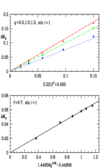
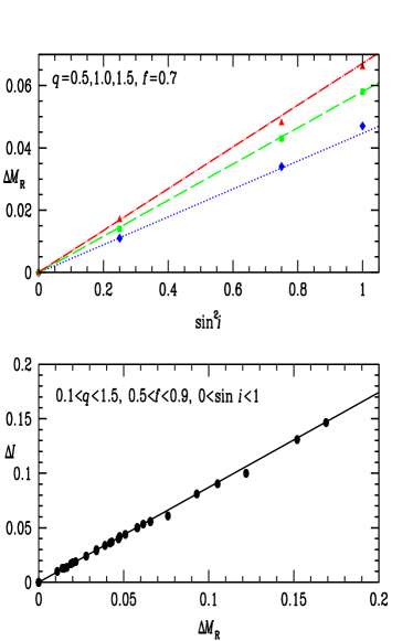
Figure 1: Fits of $\Delta M_{R}$ to the factors in Equation (9) (top three panels) and the relation between $\Delta I$ and $\Delta M_{R}$ (bottom panel). In the first and third panels, blue diamonds denote the values of $\Delta M_{R}$ when $q=0.5$, green squares denote the values of $\Delta M_{R}$ when $q=1.0$, and the red triangles denote the values of $\Delta M_{R}$ when $q=1.5$. Line fits according to Equation (9) are also shown, blue dotted lines correspond to blue diamonds, green long dashed lines correspond to green squares, and the red dot-long dashed lines correspond to red triangles. In other panels, solid circles denote the values obtained from the nightfall program and the corresponding black lines are the fits.

2.1.6 Radii during the ellipsoidal phase of the red giant evolution

Given a minimum amplitude for detectable light variations (see Section 2.1.9), the minimum radius filling factor $f_{\rm min}$ of a red giant in a binary system with detectable ellipsoidal light variation can be determined from Equations (9) and (10) after $q$ and $i$ have been selected. The corresponding minimum red giant radius $R_{\rm min}$ is given by

$$R_{\rm{min}}=R_{\rm{L}}\times{f_{\rm min}}~{}~{},$$ (11)

where $R_{\rm{L}}$ is the equivalent radius of the Roche lobe (Eggleton, 1983):

$$\frac{R_{\rm{L}}}{a}=\frac{0.49q^{-2/3}}{0.6q^{-2/3}+ln(1+q^{-1/3})}~{}.$$

The maximum stellar radius $R_{\rm{max}}$, corresponding to the Roche lobe being filled, will be

$$R_{\rm{max}}=R_{\rm{L}}~{}~{}.$$ (12)

2.1.7 Roche lobe overflow

The further expansion of a Roche lobe-filling red giant as it evolves will cause Roche lobe overflow. Then, provided the mass ratio $q=m_{2}/m_{1}$ is smaller than the critical mass ratio $q_{\rm crit}=(m_{2}/m_{1})_{\rm crit}$ for the unstable mass transfer (see below), the binary components will come into contact and undergo a CE event.

In binaries that undergo a CE event, there are two possible outcomes – a close binary system or a single coalesced star. Following widely used procedures (e.g. see Section 2.7.1 of Hurley et al., 2002), we assume that the orbital energy dissipated in the interaction process goes into overcoming the binding energy of the red giant envelope which is thus lost. If neither the remnant red giant core nor the companion main sequence star fills its Roche lobe at the end of this process, a close binary containing a white dwarf (the red giant core) and a main sequence star will be left. However, if the main sequence star fills its Roche lobe, then Roche lobe overflow will cause the main sequence star to mix with the common envelope. The red giant core thus gains H-rich material and the result will be a single, merged red giant whose further evolution will produce a PN with a single-star nucleus. Note that as the red giant core is much more compact than the main sequence star, it is unlikely that this core will fill its Roche lobe.

The above possibilities are treated in our model using equations (69)–(77) of Hurley et al. (2002), with $\lambda=0.5$ and $\alpha_{\rm CE}=1$ in our standard model. According to de Kool (1990, 1992); Yungelson et al. (1993) and Han, Podsiadlowski, & Eggleton (1995a), $\alpha_{\rm CE}=1$ gives the best fit to observations (we also try lower values - see Section 4). We assume the mass of the red giant core is given by the formulae $L/{\rm L_{\odot}}=59250\times(M_{\rm c}/{\rm M_{\odot}}-0.48)$ for AGB stars and $L/{\rm L_{\odot}}=5.3\times 10^{5}(M_{\rm c}/{\rm M_{\odot}})^{6.667}$ for RGB stars, which are the fits to the core mass–luminosity relation on the red giant branch shown by the evolutionary tracks of Bertelli et al. (2008) at metallicity Z=0.008.

To check when stable mass transfer rather than a CE event occurs, we use equation (57) of Hurley et al. (2002) to calculate $q_{\rm crit}$. Note that this equation assumes conservative mass transfer which we also assume. Except for small envelope masses (less than 20% of the red giant mass), the critical mass ratio $(m_{2}/m_{1})_{\rm crit}$ given by the above equation is greater than 1.0 and very few of red giants end up with stable mass transfer in our standard model. Very high mass loss rates or different values of $q_{\rm crit}$ can give larger numbers of red giants with stable mass transfer (see Section 4 where we run models with a lower value for $q_{\rm crit}$).

In binaries that undergo stable mass transfer, the red giant evolves closely filling its Roche lobe and transferring matter to its companion. Roche lobe filling is maintained in the models by enforcing a large mass transfer rate when the red giant radius exceed its Roche lobe radius. This is done using equation (2) of Chen & Han (2008).

2.1.8 Effective temperature and bolometric magnitude

Low-mass stars evolve through the RGB and later ascend the EAGB and AGB. When stars enter the EAGB and AGB they are oxygen rich. However, after several thermal pulses, which lead to dredge–up of carbon to the stellar atmosphere, the O-rich stars are converted to C-rich stars. This leads to a decrease in effective temperature $T_{\rm eff}$. Owing to this, $T_{\rm eff}$ values are calculated separately for these two sub-types.

We use the intermediate age LMC globular cluster NGC 1978 as a template for LMC red giant properties. According to the data of Kamath et al. (2010), the giant branch slope in the HR diagram for O-rich stars is given by $d\log T_{\rm eff}$/$dM_{\rm bol}=0.035$. Moreover, from the evolutionary tracks of Girardi et al. (2000), we find $d\log T_{\rm eff}$/$dm=0.03$ (with $m$ in solar masses). The effective temperature of O-rich stars is thus given by

$$\log\emph{T}_{\rm eff}=\log\emph{T}_{\rm eff,0}+0.035M_{\rm bol}+0.03m_{1}~{}~{}.$$ (13)

To find the zero point $\log\emph{T}_{\rm eff,0}$ for the effective temperature, we fit Equation (13) to the observed HR diagram (Fig. 2) for LMC sequence E stars in Soszyński et al. (2004). The effective temperatures of the observed sequence E stars are calculated by converting their $(J-K)_{0}$ to $T_{\rm{eff}}$ using the transforms in Houdashelt et al. (2000a, b). We adopt $E(B-V)$=0.08 (Keller & Wood, 2006), $E(J-K)=0.52E(B-V)$ and $A(K)=0.35E(B-V)$ (Rieke & Lebofsky, 1985). The bolometric correction $BC_{K}$ is calculated from $(J-K)_{0}$ with the transforms in Houdashelt et al. (2000a, b). The $J$ and $K$ magnitudes were obtained from the 2MASS catalogue (Cutri et al., 2003). Fitting the RGB given by Equation (13) for masses between 0.9 $\rm{M_{\odot}}$ and 1.85 $\rm{M_{\odot}}$ to the densest part of the observed RGB in Fig. 2 gives $\log\emph{T}_{\rm eff,0}=3.648$. Note that 0.9 and 1.85 $\rm{M_{\odot}}$ are the lower and upper mass limits, respectively, for low mass RGB stars (see Section 2.1.1).

There are substantial numbers of sequence E red giants in Fig. 2 which are brighter than $M_{\rm bol}=-3$ and which have $\log\emph{T}_{\rm eff}$ about 0.08 larger than that of the low mass RGB stars. These red giants are intermediate mass stars ($M>1.85\,\rm{M_{\odot}}$) with non-degenerate He cores evolving to the point of He core burning or perhaps on the EAGB. Other sequence E red giants with large deviations in $\log\emph{T}_{\rm eff}$ from the main locus of the RGB in Fig. 2, such as those in the lower right of the figure, presumably have photometry contaminated by spatially coincident field stars of the LMC or the Galaxy or they may be high mass loss rate AGB stars with thick obscuring circumstellar shells.

Because C-rich stars are often surrounded by substantial dust shells that cause an unknown amount of reddening, it is not possible to use observed photometric colors to derive the photospheric temperature. We therefore use red giant models to obtain the position of the C-rich star giant branch. For C-rich stars, the slope of the giant branch in the HR diagram is obtained from Table 5 in Kamath et al. (2010). The models in this table were computed to fit the O-rich giant branch in NGC 1978, as well as allowing for C/O ratios to increase from unity at luminosities brighter than the transition luminosity for O to C-rich stars. The models predict that $d\rm{log~{}\emph{T}_{eff}}$/$d\rm{\emph{M}_{bol}}$=0.125 for C-rich stars of mass $\sim$1.55 $\rm{M_{\odot}}$. If we adopt the distant modulus to the LMC of 18.54 (Keller & Wood, 2006), the transition luminosity from the O-rich to C-rich stars is

$$M_{\rm{bol}}=-3.57-0.6m_{1}~{},$$

based on the data of Frogel et al. (1990) and Vassiliadis & Wood (1994). Matching the effective temperature for O-rich and C-rich stars at the transition luminosity, the effective temperature of C-rich stars becomes

$$\rm{log~{}\emph{T}_{eff}=3.969+0.084\emph{m}_{1}+0.125\emph{M}_{bol}}~{}~{}.$$ (14)

With $L=4\pi\sigma R^{2}T_{\rm{eff}}^{4}$ and $\rm{log~{}{\emph{L}/L_{\odot}}=-0.4{(\emph{M}_{bol}-4.75)}}$, we can derive the bolometric magnitude for O-rich and C-rich stars as a function of stellar radius $R$ from Equations (13) and (14). For O-rich stars,

$$M_{\rm{bol}}=4.362-0.222m_{1}-3.704\rm{log}\emph{R}~{}~{},$$ (15)

and for C-rich stars,

$$M_{\rm{bol}}=1.189-0.373m_{1}-2.222\rm{log}\emph{R}~{}~{}.$$ (16)

If we substitute $R$ with $R_{\rm{min}}$ or $R_{\rm{max}}$, then we get the minimum or maximum bolometric magnitude of the red giants with just-detectable light variations or with Roche lobes that are just full, respectively. We note that the formulae given above for $T_{\rm eff}$ are derived from single star observations. However, these formulae should also give good results for red giants in binary systems as stellar radii are not greatly affected by the presence of a binary companion (Paczyński, 1971, and references therein).

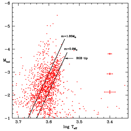
Figure 2: The HR diagram of the sequence E stars. The red points are the observation data, while the black lines are the red giant branch fits for masses of $0.9~{}\rm{M_{\odot}}$ and $1.85~{}\rm{M_{\odot}}$. Typical observational error bars are shown at three magnitude levels. The maximum luminosity of each black line corresponds to the transition luminosity from O-rich to C-rich stars. The luminosity of the RGB tip is also marked.

2.1.9 The MACHO and OGLE comparison data

As noted in the introduction, Wood et al. (1999) and Soszyński et al. (2004) found that the fraction of red giants which have detectable ellipsoidal variability is $\sim$0.5% and 1–2%, respectively. The higher fraction found by Soszyński et al. (2004) is due to the smaller photometric errors of the OGLE observations and hence the ability of OGLE to detect smaller ellipsoidal variations than MACHO. The fraction of stars that show ellipsoidal variability is an important input to our calculations, so we recompute these fractions accurately. We also investigate the amplitude required for detectability of ellipsoidal variability in each of these two studies.

Using the MACHO data of Wood et al. (1999) and selecting the top one magnitude of the RGB, we find that the fraction of red giants with detectable ellipsoidal variability is 0.61%. Similarly, using the OGLE II ellipsoidal variables on the top one magnitude of the RGB from Soszyński et al. (2004) and the corresponding total red giant population from Udalski et al. (2000), we find an ellipsoidal fraction of 1.33%.

The distributions of full light amplitude for the MACHO and OGLE II ellipsoidal variables are shown in Fig. 3. It is clear that the OGLE II observations detect variability at considerably lower amplitude than the MACHO observations. Also shown in Fig. 3 are the corresponding distributions of ellipsoidal light amplitudes on the top one magnitude of the RGB computed from our Monte Carlo model. We take the detectability limits for ellipsoidal variability to be the light amplitude at which the observed number of stars has fallen to 50% of the estimated true number. These limits are 0.055 magnitudes for the $M_{R}$ band data and 0.019 magnitudes for the OGLE $I$ band data. We use these detectability limits and the observed relative fractions of ellipsoidal variables to calibrate our Monte Carlo model.

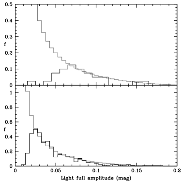
Figure 3: The relative distribution of full light amplitude for ellipsoidal variables on the top one magnitude of the RGB. Grey lines are estimates from the Monte Carlo simulation and the black lines are the observed OGLE II distribution from Soszyński et al. (2004) (bottom panel) and the observed MACHO distribution from Wood et al. (1999) (top panel). The histograms in the top panel apply for the MACHO red band while the histograms in the bottom panel apply for the OGLE II $I$ band.

2.1.10 A summary of evolutionary outcomes

We aim to predict the fractions of binary and single red giant stars that suffer each of the various possible evolutionary fates. The possible evolutionary outcomes are itemized below.

1. The star reaches the AGB tip without filling its Roche lobe. Single stars will follow this path and produce a single PN. Wide and intermediate period binaries will also follow this path, producing a PN with its nucleus in a wide or intermediate period binary.

2. The star fills its Roche lobe on the AGB but above the RGB tip. There are three possible outcomes.

   1. A CE event leads to the formation of a close binary consisting of an AGB star core and a secondary star. In this case, evolution of the AGB star core leads to creation of a PN with a close binary nucleus.

   2. A CE event leads to a merger of the two stars with the secondary star merging into the red giant envelope. The merged star will then evolve to the AGB tip as a single star.

   3. Stable mass transfer occurs leading to the formation of an intermediate period binary. If all the mass lost from the red giant was transferred to the secondary, no PN would be visible. However, there is likely to be some mass lost from the system and we assume a PN will be seen in the rare cases that stable mass transfer occurs.

3. The star fills its Roche lobe below the RGB tip. For stars with initial masses $m<1.85~{}\rm{M_{\odot}}$, the Roche lobe filling will occur on the RGB. However, for stars with $m>1.85~{}\rm{M_{\odot}}$, this will occur on the EAGB. There are three possible outcomes of such CE events.

   1. A CE event leads to the formation of a close binary consisting of a red giant core and a secondary star. In this case, evolution of the red giant core to high effective temperatures is too slow to lead to creation of a PN (see the post-RGB evolution tracks of Driebe et al. (1998) but note the comments at the beginning of Section 3; the cores of EAGB stars also evolve slowly as they are burning He in a shell). We will generally call these stars post-RGB stars even though some of them come from the EAGB. Theoretical considerations suggest that the outcome of a CE event in a close binary on the RGB (or EAGB) is likely to be a post-CE binary consisting of a low-mass He-core (or CO-core) white dwarf and a basically unaltered low-mass secondary (Paczynski, 1976; Webbink, 1984). We suggest that some Population II Cepheids, UU Herculis variables and RV Tauri stars with luminosities below the RGB tip are also formed in this way. Most, if not all, RV Tauri stars are binary systems that have mid-infrared dust emission and circumbinary disks (de Ruyter et al., 2005; Lloyd Evans & van Winckel, 2007), as expected from terminating red giant evolution on the RGB or AGB by Roche lobe filling. Observationally, some of the Population II Cepheids, UU Herculis variables and RV Tauri stars in the LMC have luminosities below the RGB tip luminosity (Alcock et al., 1998).

   2. A CE event leads to a merger of the two stars with the secondary star merging into the red giant envelope. The merged star will then evolve to the AGB tip as a single star.

   3. Stable mass transfer occurs leading to the formation of an intermediate period binary. Some of the binary Population II Cepheids, UU Herculis variables and RV Tauri stars with dust disks could be produced in this way.

2.1.11 Simulation normalization

We use the well determined fractions of the sequence E stars on the top one magnitude of the RGB (Section 2.1.9, Wood’s 0.61% and Soszyński’s 1.33%) to normalize our calculations. Given our adopted IMF, period distribution and mass ratio distributions, some binary stars will have parameters such that the Roche lobe fills or nearly fills at these luminosities ($-2.6>M_{\rm bol}>-3.6$), and the star will exhibit detectable ellipsoidal light variations characteristic of sequence E stars over a luminosity sub-interval of one magnitude. The lifetime as a sequence E star, corresponding to this luminosity sub-interval, is calculated by using the evolutionary rate described in Section 2.1.3. Some of the other binaries will have their evolution terminated by interaction before reaching $M_{\rm bol}=-2.6$ and some will evolve through the full interval without showing any detectable light variations. In the latter case, the lifetime is also calculated using the evolutionary rate described in Section 2.1.3. We calculate and sum the sequence E lifetimes of all RGB and EAGB stars in the interval $-2.6>M_{\rm bol}>-3.6$ and we also calculate and sum the total lifetimes of all red giants as they pass through this interval. The ratio of the summed sequence E lifetimes of those binaries showing detectable ellipsoidal variations to the total summed lifetimes of all binaries gives the apparent fraction of sequence E stars. This apparent fraction due to binaries alone is always greater than the observed fraction. Therefore, after we have considered $10^{6}$ binary stars in the Monte Carlo simulation, we add single stars to the population of stars, assuming they evolve through the full interval $-2.6>M_{\rm bol}>-3.6$, until the predicted and observed sequence E fractions match. Note that we are implicitly assuming here that the ratio of binary to single stars in the LMC is a free parameter and that it can differ from the ratio estimated for stars in the solar vicinity. According to Duquennoy & Mayor (1991) the percentage of solar-type stars that are single is $\sim$33% while Raghavan et al. (2010), who derive a period distribution quite similar to that of Duquennoy & Mayor (1991), estimate the percentage of single solar-type stars to be $\sim$56%.

We emphasize that our main purpose in this study is to use the observed sequence E star population, which has initial orbital periods of $\sim$100-600 days, to estimate the population of red giants whose evolution is affected by binary interactions. These interacting stars typically have initial orbital periods of $\la$3000 days. The observed period distribution of binary stars (Duquennoy & Mayor, 1991; Raghavan et al., 2010) is very broad with a peak at $\sim$$10^{5}$ days and the stars we are primarily concerned with occupy only a small part of the overall period distribution. Our predictions related to red giant evolution should thus be relatively insensitive to the overall period distribution (provided it is smooth). However, estimates of the numbers of stars with periods $>>$3000 days, and the number of single stars, will depend more sensitively on the overall period distribution.

3 Results for the standard model

In this section, we present the results for our standard model using both the Wood and Soszyński frequencies for sequence E stars. The models produce the relative birthrates of stars that terminate their AGB or RGB evolution. The numbers in Table 1 give these relative birthrates.

Throughout this paper we make some assumptions. Firstly, we assume that all stars that leave the AGB produce a PN. Secondly, when we compare ratios of populations of different types of PNe (for example close binaries PNe and all PNe) we assume that the PN lifetimes is independent of the AGB termination process (CE event or wind) although this may not be the case (e.g. Moe & De Marco, 2006) . Similar considerations apply for the post-RGB stars. It should be kept in mind that we are really comparing birth rates.

An example of how evolution rates could be different for post-CE stars and single or non-interacting binaries is provided by the class of post-AGB (perhaps post-RGB) star that consists of a binary system with a dusty circumbinary disk, an orbital period of a few hundred days or more, and a large eccentricity (van Winckel, 2007). These stars could result from AGB or RGB termination by stable mass transfer. Alternatively, their evolutionary path could be caused by the high eccentricity of their orbits. The disks around these stars may provide a reservoir of hydrogen that can be accreted back onto the high luminosity star to fuel nuclear burning for an extended period, at the same time keeping the hydrogen envelope thick enough to maintain a relatively low $T_{\rm eff}$ which is insufficient to excite a PN.

At the other extreme is the possibility that a common envelope event in a RGB star can remove enough of the hydrogen above the burning shell that the star comes out of the CE event with $T_{\rm eff}$ large enough to excite a PN almost immediately (Moe & De Marco, 2006). In our modelling, we assume that this does not happen and that the evolution of post-RGB stars is so slow that the circumstellar shell has dispersed before $T_{\rm eff}$ reaches values high enough to produce a PN (see Section 2.1.10, item 3a).

3.1 Fractions of binary planetary nebula nuclei and post-RGB stars

With the standard inputs and the evolutionary scenarios described above, we examine which binary systems form close binary PNe, intermediate period binary PNe, wide binary PNe, single binary PNe, and post-RGB binaries. The predicted PNe fractions of the standard model are listed in the first two lines of Table 1. In the total population of planetary nebula nuclei (PNNe), close binaries make up 9% or 7%, intermediate period binaries make up 27% or 23%, wide binaries make up 55% or 46%, and single stars make up 3% or 19%, using Wood’s (0.61%) or Soszyński’s (1.33%) frequency, respectively. The ratio of post-RGB star births to close binary PNNe births is $\sim$50%. Of those binaries undergoing a CE event on the AGB, we find $\sim$1.4% suffer a merger while the remainder produce a close binary. Due to the relatively higher binding energy of stars on the RGB, the frequency of mergers happening on the RGB is much higher than that on the AGB. Below $M_{\rm bol}\sim-1.5$, essentially all red giants with a main sequence companion merge when Roche lobe overflow occurs. However, if the companion is a white dwarf, a double degenerate binary can be produced down to low luminosities. Our standard model predicts that merged stars, which are likely to be rapidly rotating red giants, would make up about 5% of the red giants on the RGB above $M_{\rm bol}\sim-1.5$. Lower on the giant branch, the merged fraction will be less than 5%. Carlberg et al. (2011) estimate the observed fraction of rapidly rotating red giants to be $\sim$2%.

Our results can be compared to the binary evolution models of Han et al. (1995a). Their models 4 and 11 have input parameters similar to our standard model except that our initial period distribution is different from theirs (they assume a constant number of binaries per interval of $\log a$, where $a$ is the binary separation). In our standard model, we find that about 8% of PNNe are close binaries whereas Han et al. (1995a) predict that about 4–5% of PNNe are close binaries (see the column “CE Ejection (AGB)” in Table 1 of Han et al. (1995a) and column “Binary PNNe / CE” in this paper). The reason for our higher fraction can be traced to the different initial period distributions. Binary systems that undergo CE ejections on the AGB have initial orbital periods of about 230–1400 days or separations of about 230–760 R_⊙ (assuming the binary component masses are $\sim$1.5 M_⊙). All binary systems with initial periods (or separations) greater than these values will produce PNe through wind mass loss, as will single stars. The number of binaries with initial periods (or separations) that lead to a CE event on the AGB, relative to the number of all binaries plus single stars that produce PNe, is roughly twice as large in our standard model as in models 4 and 11 of Han et al. (1995a). This explains the higher fraction of close binary PNNe produced in our standard model. (We note that our models 15 and 16, described in Section 4, have similar period distributions to models 4 and 11 of Han et al. (1995a). Both sets of models predict that about 4–5% of PNNe are close binaries indicating similar outcomes for similar input physics.)

Finally, we note that the fractions of close binary PNNe given by Han et al. (1995a) are somewhat arbitrary since these fraction depends on the maximum binary separation allowed for their binary systems (they adopt, without giving justification, a maximum separation of $5.75\times 10^{6}$ R_⊙). They also make the assumption that there are no single stars. In our models, the fraction of stars that are single or in wide or intermediate period binaries is observationally constrained by the fraction of stars showing ellipsoidal variability on the RGB.

We now examine observational estimates of the fraction of close binary PNe. Searches carried out by Bond and collaborators for close binary central stars of PNe using photometric variability techniques obtained a fraction of 10–15% for close binary PNe (Bond & Grauer, 1987; Bond, Ciardullo, & Meakes, 1992; Bond, 1994, 2000). However, the survey bias is not well understood since the PNe samples were monitored over 30 years with many different observing campaigns (De Marco, Hillwig, & Smith, 2008). A new survey for close binary central stars by Miszalski et al. (2009) got a fraction of 12–21% for close binary PNe. This survey is more efficient and was carried out in a relatively uniform manner, by searching for periodic photometric variability of homogeneous PNe samples. However, their 12–21% is not a definitive fraction for close binary central stars. For example, the four close binary central stars PHR 1744-3355, PHR 1801-2718, PHR 1804-2645 and PHR 1804-2913 in the Miszalski et al. (2009) sample of 22 have been subsequently questioned and excluded by Miszalski et al. (2011) which would reduce their close binary fraction to 10–16%. On the other hand, accounting for the effect of orbital inclination on the light curve amplitude, the derived close binary fraction could increase.

Our standard model prediction of $\sim$7–9% for close binary PNe, is lower than the fractions estimated from the observations mentioned above. However, our simulation is strongly constrained by the observed fractions of sequence E stars. In addition, our model reproduces the observed light amplitude, period and velocity amplitude distributions of sequence E stars as well as the fraction of low mass He white dwarfs in the total white dwarf population (see Section 3.3.2). This suggests that our estimated fraction of PNe with close binary central stars is reliable.

Table 1: Model parameters and relative birthrates of red giant progeny

Model parameters										PNNe (%)									Post-RGB stars (%)
										Single PNNe					Binary PNNe				Binaries
No	$\alpha_{\rm CE}$	$P_{\rm max}$	$R_{\rm burst}$	IMF	Pdist	$q_{\rm dist}$	B	$q_{\rm crit}$		Single	Wide	MgAGB	MgRGB		IntP	Stable	CE		CE	Stable	PRGB/PN
Standard model
1	1.0	500	10	S1955	DM1991	DM1991	0	H57	w	3.31	54.90	0.12	5.71		27.20	0.01	8.74		100.00	0.00	0.0448
									s	18.52	46.24	0.11	4.83		22.97	0.01	7.31		100.00	0.00	0.0375
One parameter variation models
2	0.6	500	10	S1955	DM1991	DM1991	0	H57	w	1.67	55.00	0.55	7.28		27.21	0.01	8.28		100.00	0.00	0.0275
									s	17.18	46.28	0.46	6.10		22.95	0.01	7.01		100.00	0.00	0.0233
3	0.3	500	10	S1955	DM1991	DM1991	0	H57	w	0.00	54.99	1.83	8.81		27.31	0.01	7.05		100.00	0.00	0.0101
									s	16.62	45.97	1.50	7.29		22.73	0.01	5.88		100.00	0.00	0.0085
4	1.0	$+\infty$	10	S1955	DM1991	DM1991	0	H57	w	19.77	0.00	0.13	5.89		65.38	0.01	8.81		100.00	0.00	0.0461
									s	33.00	0.00	0.11	4.86		54.59	0.01	7.44		100.00	0.00	0.0388
5	1.0	100	10	S1955	DM1991	DM1991	0	H57	w	0.00	68.71	0.13	5.80		16.62	0.01	8.72		100.00	0.00	0.0441
									s	14.55	59.29	0.11	4.80		13.93	0.01	7.31		100.00	0.00	0.0370
6	1.0	500	1	S1955	DM1991	DM1991	0	H57	w	3.08	55.46	0.07	5.71		27.99	0.08	7.61		100.00	0.00	0.0650
									s	18.67	46.68	0.06	4.78		23.35	0.07	6.41		100.00	0.00	0.0546
7	1.0	500	10	Reid02	DM1991	DM1991	0	H57	w	1.10	56.35	0.19	5.59		27.63	0.01	9.12		100.00	0.00	0.0407
									s	15.48	48.04	0.17	4.75		23.72	0.01	7.83		100.00	0.00	0.0342
8	1.0	500	10	S1955	Flat	DM1991	0	H57	w	62.15	3.91	0.11	10.45		16.37	0.01	6.99		100.00	0.00	0.0480
									s	66.87	3.42	0.11	9.10		14.39	0.01	6.11		100.00	0.00	0.0419
9	1.0	500	10	S1955	DM1991	$n(q)=q^{-0.4}$	0	H57	w	11.40	41.73	0.20	6.61		30.57	0.02	9.47		100.00	0.00	0.0533
									s	23.55	36.11	0.17	5.68		26.32	0.02	8.15		100.00	0.00	0.0461
10	1.0	500	10	S1955	DM1991	$n(q)=1$	0	H57	w	27.55	34.43	0.09	4.93		25.37	0.03	7.61		100.00	0.00	0.0447
									s	35.73	30.60	0.08	4.37		22.50	0.02	6.70		100.00	0.00	0.0398
11	1.0	500	10	S1955	DM1991	$n(q)=q$	0	H57	w	37.00	30.58	0.03	3.69		22.62	0.04	6.05		100.00	0.00	0.0439
									s	41.04	28.62	0.02	3.43		21.13	0.04	5.71		100.00	0.00	0.0411
12	1.0	500	10	S1955	DM1991	DM1991	500	H57	w	8.16	52.63	0.10	5.33		27.32	0.73	5.74		99.30	0.70	0.0478
									s	19.65	45.97	0.09	4.71		23.96	0.63	4.98		99.28	0.72	0.0420
13	1.0	500	10	S1955	DM1991	DM1991	0	0.8	w	23.07	43.35	0.10	4.42		21.79	0.72	6.55		92.18	7.82	0.0367
									s	26.68	41.35	0.10	4.26		20.74	0.68	6.19		92.02	7.98	0.0351
Multiple parameter variation models
14	1.0	500	10	S1955	R2010	$n(q)=1$	0	H57	w	16.38	42.63	0.10	4.77		28.20	0.03	7.88		100.00	0.00	0.0450
									s	26.15	37.63	0.08	4.23		24.92	0.02	6.96		100.00	0.00	0.0399
15	1.0	100	1	MS1979	Flat	$n(q)=1$	0	H57	w	63.43	8.96	0.05	11.00		10.79	0.10	5.67		100.00	0.00	0.0720
									s	66.63	8.13	0.05	10.12		9.73	0.12	5.23		100.00	0.00	0.0650
16	1.0	100	1	MS1979	Flat	$n(q)=q$	0	H57	w	71.36	7.44	0.01	7.96		8.91	0.13	4.19		100.00	0.00	0.0654
									s	71.99	7.29	0.02	7.71		8.66	0.13	4.21		100.00	0.00	0.0630
17	1.0	500	10	S1955	DM1991	DM1991	500	0.8	w	26.15	42.00	0.08	4.24		22.16	1.59	3.77		86.64	13.36	0.0420
									s	28.44	40.62	0.08	4.17		21.44	1.56	3.68		86.06	13.94	0.0396

Model parameters: $\alpha_{\rm CE}$ is the orbital energy transfer efficiency (see Section 2.1.7); $P_{\rm max}$ is the maximum initial period (in years) for which a binary is assumed to influence the shape of PNe; $R_{\rm burst}$ is the star formation rate burst factor (see Section 2.1.1); IMF is the assumed initial mass function (‘S1955’ from Salpeter 1955, ‘Reid02’ from Reid et al. 2002, ‘MS1979’ from Miller & Scalo 1979); P_dist is the initial period distribution (‘DM1991’ from Duquennoy & Mayor 1991, ‘R2010’ from Raghavan et al. 2010, ‘Flat’ means $dN\propto d{\rm log}P$); $q_{\rm dist}$ is the initial mass ratio distribution $n(q)\propto dN/dq$; B is the parameter in the tidally enhanced mass loss rate formula (see Section. 2.1.3); $q_{\rm crit}$ = ($m_{2}/m_{1}$)_crit is the critical mass ratio above which Roche lobe overflow is stable (‘H57’ is the value given by equation (57) of Hurley et al. 2002).
Model results: Lines containing ‘w’/‘s’ use Wood’s/Soszyński’s sequence E frequency to normalize the results. The numbers in columns 11–19 give the relative birth rates for PNNe and post-RGB stars (as a percentage). The sum of all PNNe birthrates is 100%, as is the sum of the post-RGB star birthrates. The ratio of the total post-RGB star birthrate to the total of the PNNe birth rate is given column 20. PNNe types are: stars that are born single (Single); wide binaries which have $P>P_{\rm max}$ and which do no influence the shape of their PNe (Wide); binary stars that merge on the AGB (MgAGB) or the RGB (MgRGB); intermediate period binaries that never fill their Roche lobes but which have $P<P_{\rm max}$ (IntP); binary stars that fill their Roche lobes and then undergo stable mass transfer (Stable); and binary stars that fill their Roche lobes and then undergo a CE event leaving a close binary (CE). Post-RGB are: those that result from CE events (CE); those that result from stable mass transfer (Stable).

3.2 Properties of sequence E stars

To further test our simulation, we predict the binary properties of sequence E stars and compare them with observations where possible. The main available data are the photometric variations from MACHO and OGLE experiments, which provide a probe into the period distribution. Nicholls et al. (2010) provide radial velocity observations of sequence E stars, although only 11 binary systems were studied.

3.2.1 Period distribution

In Fig. 4, we present the orbital period distribution of sequence E stars, predicted with Wood’s and Soszyński’s frequencies. The orbital period contribution of a single binary to the distribution is the average of the periods at onset and end of detectable sequence E variability on the RGB, weighted by the sequence E lifetime for the system: note that the orbital period typically changes by less than 3% during the sequence E phase (due to mass loss and tidal interaction). We also show the distribution of the observed periods, using the sample of Soszyński et al. (2004). We only consider the sequence E stars on the top one magnitude of the RGB, so the stars in the observed period distribution are selected based on their luminosity. Fig. 4 shows that the simulation reproduces the observation very well: not only are the total numbers of sequence E stars reproduced, as required, but their period distribution is reproduced as well. We also note that the shape of the light amplitude distribution is reproduced well by the model (Fig. 3).

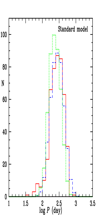
Figure 4: The orbital period distribution of sequence E stars. The red solid line denotes the distribution from the observations of Soszyński et al. (2004), the green dotted line denotes the distribution from the model using Wood’s frequency, and the blue short dashed line denotes the distribution from the model using Soszyński’s frequency.

3.2.2 Full velocity amplitude distribution

In Fig. 5, we show the full velocity amplitude distributions from our model and the radial velocity observations by Nicholls et al. (2010). The expected full velocity amplitude concentrates in the range of $\sim$5 to 50 km s^-1, with a peak at $\sim$22.5 km s^-1. It shows a reasonable agreement with the observations, although the observed number is small.

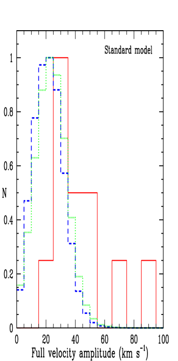
Figure 5: The full velocity amplitude distribution of sequence E stars. The red solid line denotes the distribution from the observation of Nicholls et al. (2010) with 11 stars, the green dotted line denotes the distribution from the model using Wood’s frequency, and the blue short dashed line denotes the distribution from the model using Soszyński’s frequency. The distribution peaks are normalized to 1.

3.2.3 Mass distribution

In Fig. 6, we show the mass distribution of the sequence E stars. The mass range is from 0.85–3.0 $\rm{M_{\odot}}$, with the LMC star burst beginning at 1.3 $\rm{M_{\odot}}$. The lower limiting mass of 0.85 $\rm{M_{\odot}}$ is set by the mass of the oldest stars and stellar wind mass loss. There are a large number of stars in the range of 1.3–1.85 $\rm{M_{\odot}}$, where the latter mass is the maximum mass for stars that ascend the RGB with an electron degenerate core. The more massive stars in Fig. 6 are EAGB stars at luminosities corresponding to the top magnitude of the RGB.

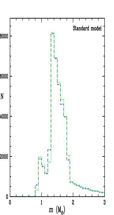
Figure 6: The mass distribution of the sequence E stars. The green dotted line denotes the distribution from the model when using Wood’s frequency while the blue short dashed line denotes the distribution from the model when using Soszyński’s frequency.

3.2.4 Mass ratio distribution

In Fig. 7, we show the mass ratio distribution of sequence E stars. The mass ratio is less than 1.1, with a peak at $\sim$0.5. Mass loss from the red giant is the reason that some systems have mass ratio slightly greater than 1.

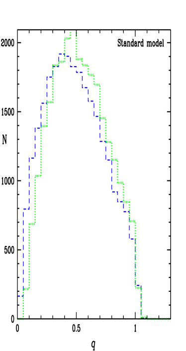
Figure 7: The same as Fig. 6 but for the mass ratio.

3.2.5 Orbital separation distribution

In Fig. 8, we show the orbital separation distribution of sequence E stars. The separation is in the range of $\sim$100–600 $\rm{R_{\odot}}$, with a narrow peak at $\sim$200 $\rm{R_{\odot}}$.

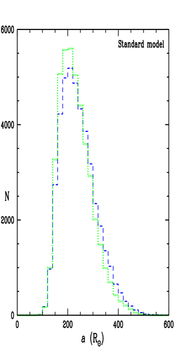
Figure 8: The same as Fig. 6 but for the orbital separation.

3.2.6 Ellipsoidal variability lifetime

We show the predicted ellipsoidal variability lifetime of sequence E stars in Fig. 9. The distribution starts at a peak of $\sim$0.2 Myr due to the contribution of EAGB stars with $m>1.85~{}\rm{M_{\odot}}$, and then falls to zero at 2 or 4 Myr. Longer lifetimes are predicted in the Soszyński case than the Wood case. The reason is that OGLE II has a more sensitive detection limit for photometric variations ($\sim$0.02 mag) than MACHO ($\sim$0.05 mag) (see Fig. 3), so Soszyński’s stars are detected initially with less-filled Roche lobes and it then takes longer before the lobe is filled and RGB evolution is terminated. The average lifetime for sequence E stars is $\sim$0.95 Myr, when the ellipsoidal variation amplitude is more than 0.02 magnitudes.

Mikołajewska (2007, 2011) claims that in symbiotic stars, the red giant radius is often close to half the Roche lobe radius yet ellipsoidal light variations are seen in these stars with an amplitude that suggests the Roche lobe is almost filled. If this claim is correct, then it suggests some unidentified source of light variation that simulates an ellipsoidal variation. The sequence E stars are not as extreme as the symbiotic stars where the red giant is usually a semi-regular or Mira variable with a large mass loss rate and the companion is a hot accreting white dwarf whose radiation may affect the facing surface of the red giant. We therefore do not expect our ellipsoidal light curve calculations for sequence E stars to be affected by an unidentified source of ellipsoidal-like light variation. Nevertheless we investigate how such an extra source would alter our results if it did exist. To simulate the extra light amplitude suggested in symbiotic stars, we replaced the Roche lobe filling factor $f$ in Equation (9) by $2f$. The effect of this is to make detectable ellipsoidal variability occur when the radius of the red giant is half the usual value. Note that this does not affect the evolution of any star, it simply means that ellipsoidal variability is detectable in red giants with wider orbits than in our usual calculations. This in turn causes a larger fraction of binaries to appear as sequence E stars. Now, in order to reproduce the observed fractions of sequence E stars, a much larger population of single stars is required than in our usual models. For example, in our standard model, about 10% of stars are single and 90% are in binaries whereas in the models with the modified Equation (9) about 80% of stars are single and 20% are in binaries. This means that the fraction of all stars that undergo CE events or mergers is reduced by a factor of $90/20=4.5$. In particular, the fraction of close binary PNNe is reduced from $\sim$8% to $\sim$1.8%. (We also note that in our modified models the ellipsoidal light amplitudes of stars nearly filling their Roche lobes are increased by a factor of 16 giving rise to ellipsoidal light curve amplitudes up to 3 magnitudes, which are never observed (see Fig. 3). Of course, the modified Equation (9) has no physical basis so we cannot really say what the ellipsoidal amplitudes should be.)

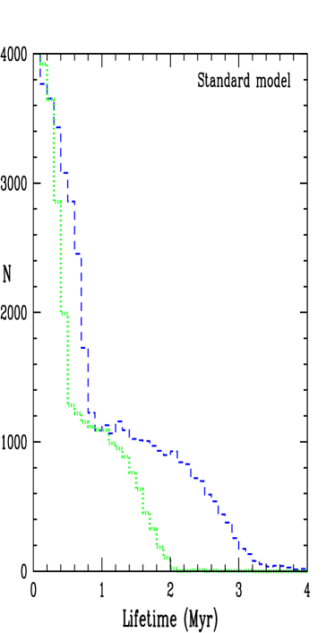
Figure 9: The same as Fig. 6 but for the lifetime of the ellipsoidal variability.

3.3 Properties of binary PNNe and post-RGB stars

3.3.1 Luminosity distribution

In Fig. 10, we show the luminosity distributions of the outcomes of the binary red giants according to the standard model. As expected, intermediate period binary PNNe have luminosities of the AGB tip, close binary PNNe have AGB luminosities above the RGB tip, and EAGB and RGB binaries undergoing a CE event but not merging have luminosities below the RGB tip. Mergers occur preferentially at luminosities lower than the luminosities of CE events that lead to binaries. The RGB binaries formed at $M_{\rm bol}\ga-1.5$ are double degenerates. In these systems, the small radius of the companion white dwarf allows them to avoid a merger.

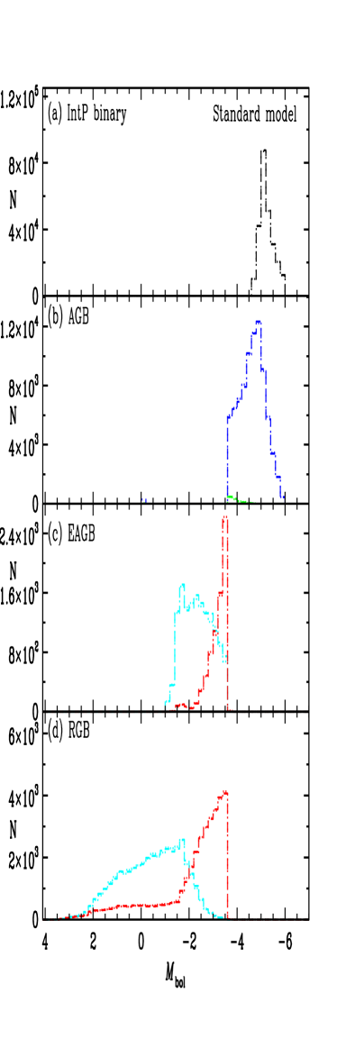
Figure 10: Luminosity distributions of binary red giants at the termination of their red giant evolution. Panel (a): intermediate period binary PNNe with $P<500$ years. Panel (b): close binary PNNe (blue) and merged AGB stars (green). Panel (c): EAGB binaries (red) and merged EAGB stars (cyan/grey). Panel (d): RGB binaries (red) and merged RGB stars (cyan/grey). In all panels, dotted lines denote the distributions from the model when using Wood’s frequency, short dashed lines denote the distributions from the model when using Soszyński’s frequency.

3.3.2 Mass distribution

In Fig. 11, we show the mass distributions of the binary red giants at their termination luminosities. As expected, stars in intermediate period binaries lose a significant amount of their mass via the Reimers-like stellar wind. Mergers occur preferentially at lower luminosity so such systems have the least mass loss.

At the end of the superwind phase or a CE event, a red giant has lost its whole envelope, leaving a He (or CO) core as a remnant. In Fig. 12, we present the mass distribution after the red giant envelope has been lost. The mass of the close binary PNNe is in the range of $\sim$0.50–0.80 $\rm{M_{\odot}}$, with most of the stars concentrated between 0.50–0.65 $\rm{M_{\odot}}$. For the post-RGB binaries, the mass is lower, with a range of $\sim$0.2–0.45 $\rm{M_{\odot}}$. The post-EAGB CO-cores concentrate around 0.50 $\rm{M_{\odot}}$. The mass distributions of intermediate period binary PNNe are also shown in Fig. 12. The masses are in the range of $\sim$0.55–0.85 $\rm{M_{\odot}}$, with a strong peak at $\sim$0.6$~{}\rm{M_{\odot}}$.

Mass determination of 86 PNNe by Stasińska & Tylenda (1990) shows a mass distribution similar to our prediction: the mass range is 0.55–0.75 $\rm{M_{\odot}}$, and most of the PNNe concentrate between 0.55–0.65 $\rm{M_{\odot}}$. Similarly, Zhang & Kwok (1993) determined the mass of 303 PNNe, reporting a mass distribution from 0.55–0.85 $\rm{M_{\odot}}$, with a narrow peak at 0.6 $\rm{M_{\odot}}$. The population synthesis model results of Yungelson et al. (1993) and Han et al. (1995a) give mass distributions of close binary PNNe (with $\alpha_{\rm CE}=1$) that are similar to ours.

For the post-RGB stars, the predicted masses are consistent with observations of low-mass white dwarf binaries. For example, Liebert, Bergeron, & Holberg (2005) and Rebassa-Mansergas et al. (2011) determined the mass distribution of local white dwarfs and found a distribution with a peak at 0.4 $\rm{M_{\odot}}$ as well as a more dominant peak around 0.6 $\rm{M_{\odot}}$ which corresponds to CO white dwarfs produced by evolution off the AGB. The low mass peak is produced predominantly by CE events on the RGB, although some of these stars ($<$30%) may be single (Kilic, Brown, & McLeod, 2010; Brown et al., 2011; Rebassa-Mansergas et al., 2011, and references therein) which requires an exotic type of evolution such as an unusually high wind mass loss on the RGB, or ejection of the envelope by a giant planet, or mergers of two He white dwarfs (we do not find any such events). The studies of Liebert et al. (2005) and Rebassa-Mansergas et al. (2011) suggest that the birth rate of low mass He white dwarfs is about 4-10% of the total white dwarf birth rate. Our standard model predicts this relative birth rate to be 9.6%, in good agreement with the observations. Our predicted mass distribution is also consistent with the observations and the simulations of Yungelson et al. (1993) and Han et al. (1995a). Note that the He white dwarfs with masses from 0.2–0.3 $\rm{M_{\odot}}$ in Fig. 12 are nearly all double degenerates and they form about 19% of the He white dwarfs. Some He white dwarfs are known to be in double degenerate systems (Marsh, Dhillon, & Duck, 1995) although the observed fraction is very poorly known (Kilic, Stanek, & Pinsonneault, 2007). Our models predict that only $\sim$0.1% of sequence E stars will have a white dwarf companion (on the way to producing a double degenerate), consistent with our finding mentioned in the introduction that there is no evidence for degenerate companions in a sample of 110 sequence E stars.

Finally, we note that our adopted star formation history means that there are no stars with initial masses greater than 3.0 M_⊙. Even if we were to allow recent star formation by (say) using $f(t)=b$ for $t<0.5$, the relative number of stars with $M>3.0$ M_⊙ would be tiny because of the combined effects of the IMF and the star formation history. We would not simply be extending the plots in Figs. 11 to higher masses according to the IMF. We would be extending the plots at a level reduced by a factor of 10 in height since the stars with mass 1.3–3.0  M_⊙ were produced during the burst.

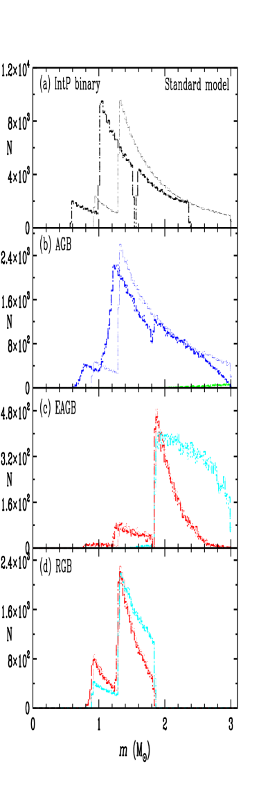
Figure 11: Mass distributions of the binary red giants according to their evolutionary fates. Thin lines are for the initial mass distributions. Thick lines are for the mass distribution at the termination luminosity: the top panel shows the mass for intermediate period binaries at the AGB tip and just before the beginning of the superwind phase; the other panels show the mass at the start of the CE event. Colors are as in Fig. 10.

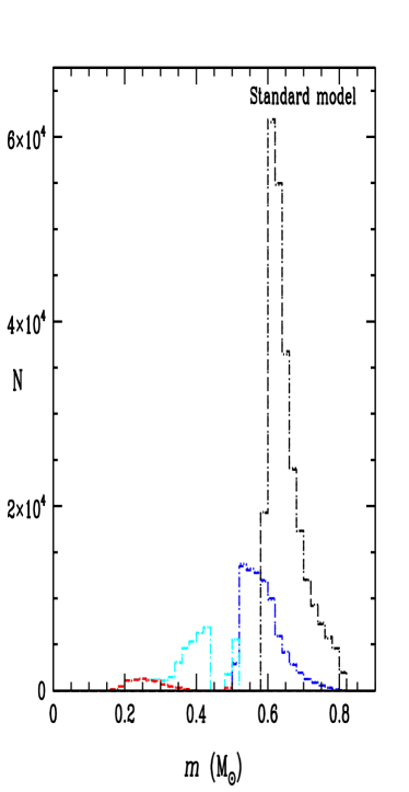
Figure 12: Mass distributions of intermediate period binary PNNe (black), close binary PNNe (blue), post-RGB and post-EAGB binaries (cyan/grey) and double degenerate secondaries (red). Note that the cyan curves include the double degenerate component.

3.3.3 Period distribution

In Fig. 13, we present the orbital period distribution of the close binary PNNe and post-RGB binaries. The orbital periods of the close binary PNNe have a range from 0.01–1000 days, and a peak at $\sim$4 days. The orbital periods of post-RGB binaries are between 0.01–10 days, and have a narrow peak at $\sim$0.3 days.

Orbital period distributions of close binary PNNe predicted by Yungelson et al. (1993) and Han et al. (1995a) have a similar distribution to ours, showing a period range of few hours to 1000 days. Observationally, periods of close binary PNNe are all less than 16 days (Bond, 2000; De Marco, 2009; Miszalski et al., 2009) with the current period distributions peaking at or below $P\sim 1$ day. This peak is at shorter periods than predicted by the model (the blue curve in Fig. 13). The absence of the long period PNNe in the current sample could be due to the observational bias against long period stars: in variability searches such as that of Miszalski et al. (2009), short periods in close binaries are needed to get the detectable light amplitudes from ellipsoidal and reflection effects; and in radial velocity searches, close binaries with short periods are needed to get the high velocity variations needed for these hot compact stars which have relatively broad lines. Alternatively, the current observed period distribution and the model period distributions can be brought into better agreement by using a lower value of $\alpha_{\rm CE}$ (see Section 4).

The orbital period distribution of local binary white dwarfs (e.g. Rebassa-Mansergas et al., 2008; Zorotovic et al., 2010) also peaks at periods less than or near 1 day. The model prediction given by the cyan line in Fig. 13 has a peak around 1 day but more stars with periods longer than 1 day than the current observational estimates.

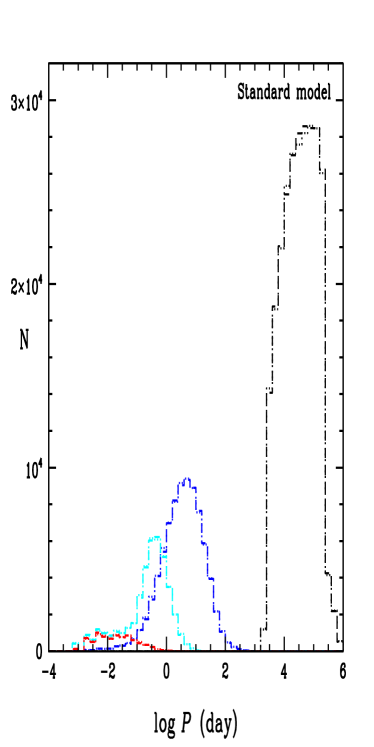
Figure 13: Orbital period distributions of the objects shown in Fig. 12. Line types are the same as in that figure.

3.3.4 Mass ratio distribution

In Fig. 14 we show the mass ratio distributions of close PNNe and post-RGB binaries. This is similar to the prediction of Han et al. (1995a).

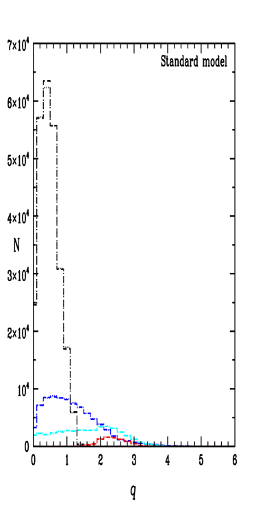
Figure 14: Mass ratio distributions of the objects shown in Fig. 12. Line types are the same as in that figure.

3.4 The population of PNe in the LMC

We use our model to predict the number of PNe in the inner 25 square degrees of the LMC searched for PNe by Reid & Parker (2006). As part of our modelling procedure to estimate the apparent fraction of sequence E stars in the top one magnitude of the RGB ($-2.6>M_{\rm bol}>-3.6$), we compute the average lifetime $\tau_{\rm 1mag}$ in this magnitude interval for all RGB and EAGB stars which evolve into this interval. We find $\tau_{\rm 1mag}=2.77\times 10^{6}$ years for the standard model, with a deviation from this value of less than 3% for other models. The average lifetime is determined by the evolution rate and variation in the average lifetime is caused by the small fraction of stars whose lives are terminated by CE events in this interval. From the SAGE catalog (Meixner et al., 2006), we obtained the near and mid-infrared photometric observations of all stars in the area searched by Reid & Parker (2006). Using the position of the giant branch in the (J,J$-$[3.6]) diagram, we selected all the stars (RGB and EAGB) in a parallelogram corresponding to the top one magnitude of the RGB. The parallelogram has sides J=13.25, J=14.25, J$-$[3.6]=$3.828-0.17{\rm J}$ and J$-$[3.6]=$3.328-0.17{\rm J}$ (see Blum et al. (2006) for SAGE colour-magnitude diagrams for the whole LMC). We found the total number of stars $n_{\rm RGB+EAGB}=58356$ and estimate an error of less than 5% in this number. The uncertainty is due to scattering of stars into and out of the parallelogram in the (J,J$-$[3.6]) diagram because of observational errors and contamination by stars at the red end of core helium burning loops. Confusion is not a problem for these relatively bright stars (see Nikolaev & Weinberg, 2000; Blum et al., 2006).

The final quantity we need in order to estimate the number of PNe in the inner 25 square degrees of the LMC is the average lifetime $\tau_{\rm PN}$ of LMC PNe. We note that there is a steep drop in the number of LMC PNe with diameters between 7 and 8 arcsec (see Fig. 16 of Reid & Parker, 2006) so we adopt 7.5 arcsec as a typical maximum diameter for LMC PNe. If we use a distance modulus to the LMC of 18.54 (Keller & Wood, 2006) and a PN expansion velocity $v_{\rm exp}$ of 34.5 km s^-1 (the median for the 94 LMC PNe in Dopita et al., 1988) then we find $\tau_{\rm PN}=2.6\times 10^{4}$ years. Using the above numbers, we predict that the number of PNe in the region surveyed by Reid & Parker (2006) will be $n_{\rm RGB+EAGB}\times\tau_{\rm PN}/\tau_{\rm 1mag}=548$ PNe. The estimated number of PNe is in good agreement with the 541$\pm$89 PNe observed by Reid & Parker (2006). Since more than 90% of these PNe come from single or non-interacting binary stars in our model, this means that most such stars produce a PN. This is contrary to the “Binary Hypothesis” (Moe & De Marco, 2006; De Marco, 2009) which suggests that binary interaction is required to produce a PN.

There are a small number of AGB star terminations that may not produce a detectable PN. Most of the single or non-interacting binary stars in our model terminate their AGB evolution by a superwind. However, some have their evolution terminated by the low mass loss rate Reimers wind. These are the stars with the lowest initial mass $0.9<{\rm M}/M_{\odot}<0.92$ which make up only 0.7% of the AGB terminations. It is these stars that may not produce a detectable PN (Soker & Subag, 2005).

4 Results for models with varied input assumptions

In order to investigate how dependent the results are on the model parameters (e.g. $\alpha_{\rm CE}$, IMF, period and mass ratio distribution), as well as to compare the results with other population synthesis calculations, we have run models with adjusted input parameters. Models have been made varying one, two or three of the parameters described above and the results are shown in Table 1. We discuss the effects on each model of varying the model parameters. For selected models, distributions of final masses and periods are plotted in Figs. 15 and 16, which are similar to Figs. 12 and 13, respectively.

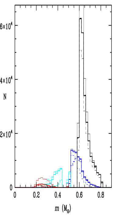
Figure 15: Mass distributions of intermediate period binary PNNe (black), close binary PNNe (blue), post-RGB and post-EAGB binaries (cyan/grey) and double degenerate secondaries (red) in models 1 (thick solid lines), 3 (thick dashed lines), 11 (thin solid lines) and 12 (thin dashed lines). Results are shown only for the models using Wood’s sequence E frequency.

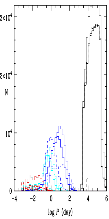
Figure 16: Orbital period distributions of the objects shown in Fig. 15. Line types are the same as in that figure.

Models 2 and 3: the energy efficiency parameter $\alpha_{\rm CE}$.
The value of the energy efficiency parameter $\alpha_{\rm CE}$ is controversial and there is no consensus for its value. As noted in Section 2.1.7, a value of 1.0 seems consistent with some observational constraints. However, smaller values of $\alpha_{\rm CE}$ have also been derived along with estimates of dependency on the parameters of the binary (Politano & Weiler, 2007; Zorotovic et al., 2010; De Marco et al., 2011; Davis, Kolb, & Knigge, 2011). To investigate the effect of changes to $\alpha_{\rm CE}$ on our modelling results, the standard value of 1.0 was changed to 0.6 and 0.3 in models 2 and 3, respectively. As expected, decreasing $\alpha_{\rm CE}$ causes more mergers to occur at the expense of fewer CE events (Table 1). Reducing $\alpha_{\rm CE}$ from 1 to 0.3 changes the fraction of close binary PN produced from $\sim 8$% to $\sim 6.5$%. The results for model 3 are shown in Figs. 15 and 16. The most interesting thing about these plots is that the periods of the close binary PNNe now peak just shortward of 1 day, in much better agreement with the current observed period distribution. A lower value of $\alpha_{\rm CE}$ is a way of removing the discrepancy between the observed period distribution and the period distribution predicted by our standard model.

Models 4 and 5: The upper limiting period $P_{\rm max}$.
$P_{\rm max}$ has been changed from the standard value of 500 years to infinity or 100 yrs. The latter value was used by Han et al. (1995a). The main effect of this parameter is to shift stars between the intermediate period, wide and single categories.

Model 6: The star burst ratio $R_{\rm burst}$.
In this model, the star burst ratio $R_{\rm burst}$ in Section 2.1.1 was changed to 1.0 to simulate a constant star formation rate, which is often used in models (de Kool, 1990, 1992; Yungelson et al., 1993; Han et al., 1995a; Politano & Weiler, 2007). The change produces more stars of mass less than 1.3 M_⊙ relative to higher mass stars. The effect is a small reduction in the number of CE events on the AGB and an increase in the number of CE events on the RGB. This is probably due to the smaller initial orbital separations of the lower mass binaries, given that the same period distribution is assumed at all masses.

Model 7:The IMF.
Here the Salpeter IMF was changed to the Reid, Gizis, & Hawley (2002) power law (with an exponent of $-1.3$). The effect on the birthrate ratios is small, with slightly more CE events on the AGB and fewer on the RGB.

Model 8: The period distribution $P_{\rm dist}$.
Here a flat period distribution with $dN\propto{d\,\rm{log}\emph{P}}$ was used. This period distribution has been commonly used (see de Kool, 1990, 1992; Han et al., 1995a). The period distribution has a large influence on the relative birthrates of single, wide and intermediate period PNNe. Since the flat period distribution has far fewer stars born at long periods relative to the periods of the sequence E stars, it is necessary to add many more single stars than in the standard model in order the get the fraction of sequence E stars on the top magnitude of the RGB to agree with the observational value. The fraction of stars undergoing CE events is slightly lower than in the standard case. This model is a good indicator of the fact that using sequence E stars to normalize our results keeps the fraction of CE events in our simulations fairly constant when model parameters are changed.

Models 9 to 11: Mass ratio distributions $q_{\rm dist}$.
Initial mass ratio distributions $n(q)=Cq^{a}$ with $a=-0.4$, 0 or 1 were tried. The first exponent was that found by Kouwenhoven et al. (2007) for main-sequence A and B stars ($M\sim 2-15$ M_⊙) in the Sco OB2 association. The higher the fraction of high mass companions, the fewer the number of mergers, as might be expected from the higher orbital energy available to eject the red giant envelope. The higher the fraction of high mass companions also gives a smaller percentage of CE events in our model. This is probably because, for a given fraction of sequence E stars, a higher mass companion can give a detectable ellipsoidal light variation at a larger orbital separation, reducing the likelihood of a CE event occurring. The final mass and period distributions for model 11 are shown in Figs. 15 and 16. These plots clearly show an increase in the fraction of double degenerates produced when the number of high mass companions is increased. The periods of the close binary PNNe are also increased slightly.

Model 12: Tidally enhanced mass loss.
The tidally enhanced mass loss rate of Tout & Eggleton (1988) was tried, with the free parameter ‘$B$’ set to 500, although its actual value is very uncertain (Han et al., 1995b; Han, 1998; Soker et al., 1998; Karakas, Tout, & Lattanzio, 2000; Frankowski & Tylenda, 2001; Hurley et al., 2002). The main effect is an increase in the number of stars undergoing stable mass transfer (because of the increase in $m_{2}/m_{1}$ resulting from mass loss from the red giant) and a decrease in the number of CE events. The final mass and period distributions for model 12 are shown in Figs. 15 and 16. The reduced number of CE events on the AGB is clearly evident in the figures. There is also an extension of the period distribution of close binary PNNe to higher values, further increasing the discrepancy between the observed and predicted period distributions. The enhanced mass loss also significantly increased the minimum period of intermediate period PNNe.

Models 13 and 17: Critical mass ratio $q_{\rm crit}$.
The critical mass ratio $q_{\rm crit}=(m_{2}/m_{1})_{\rm crit}$, above which mass transfer from a Roche lobe filling red giant is stable, has some uncertainty. Chen & Han (2008) investigated the value of $q_{\rm crit}$ appropriate for mass transfer from red giants under various conditions. For the more luminous stars and for mass transfer efficiencies more than 0.5, the value of $q_{\rm crit}$ is mostly similar to that used here in our standard model. However, values as low as $(m_{2}/m_{1})_{\rm crit}=0.8$ are found by Chen & Han (2008) in some cases. In order to see how dependent our models are on $q_{\rm crit}$, we ran a simulation with $q_{\rm crit}=0.8$. We also ran a simulation with $q_{\rm crit}=0.8$ and ‘$B$’ = 500 to see how the extra reduction in the red giant mass from the enhanced mass loss would affect the number of stars undergoing stable mass transfer. As expected, the number of stars undergoing stable mass transfer is greatly increased, especially on the RGB. The fraction of binaries undergoing CE events is decreased because of the alternative evolutionary path for Roche lobe filling stars. Changing $q_{\rm crit}$ to 0.8 makes no significant difference to the mass and period distributions.

Model 14: The Raghavan et al. (2010) distributions.
Here we use the period and mass ratio distributions of Raghavan et al. (2010) which can be considered as updated versions of the distributions of Duquennoy & Mayor (1991). Raghavan et al. (2010) have a period distribution similar to that of Duquennoy & Mayor (1991) but they have a flat mass ratio distribution. The results are very similar to those of model 10 which also has a flat mass ratio distribution.

Models 15 and 16: The Miller & Scalo (1979) IMF.
Here we use the Miller & Scalo (1979) lognormal IMF appropriate for low-mass stars, combined with a flat period distribution, and $n(q)=1$ or $q$. Our model 15 has similar parameters to model 4 of Han et al. (1995a). As with model 8, the flat period distribution leads to a high single star fraction in our simulation. The combined effect of all parameters is to decrease the number of CE events on the AGB and increase the number on the RGB.

5 Conclusions

We have used the population of red giants that are ellipsoidal variables in the LMC to predict the fates of binary red giants. In our standard model, we found 7–9% of PNe contain close binaries, 23–27% contain intermediate period binaries ($P<500$ years) capable of influencing the shape of a PN, 46–55% contain wide binaries, 5–6% are from merged stars and 3–19% are from single stars. The production rate of post-RGB stars, consisting of a He white dwarf and a low-mass secondary, is $\sim$50% of the production rate of close binary PNNe.

Our predicted fraction of close binary PNe (7-9%) is somewhat lower than current observational estimates of 10-20%. Similarly, the observed orbital period distribution for close binary central stars of PNe has few stars with periods more than 1 day whereas the models predict that there should be a significant population of binaries with periods out to 100 days. The periods predicted by the models can be brought into better agreement with the currently observed periods by reducing $\alpha_{\rm CE}$. The current observational samples are small and detection techniques work best for short period systems. Larger samples and different detection techniques are needed to improve the significance of the current observational estimates.

The mass distribution of all white dwarfs produced shows two peaks around 0.4 and 0.6 M_⊙ corresponding to He and CO white dwarfs, respectively. The birth rate of He white dwarfs is predicted to be about 10% of the total white dwarf birth rate, in agreement with the observed birth rate ratio.

We estimate that about one third of PNe contain binaries capable of influencing the shape of the nebula (the close and intermediate period binaries), a significantly smaller fraction than the observed fraction of non-spherical PNe which is $\sim$80%. This indicates that mechanisms other than binarity are responsible for shaping PNe, such as stellar rotation, magnetic fields or planets (see De Marco, 2009, for a review).

Using our model and the observed number of red giant stars on the top one magnitude of the RGB, we predict that the number of PNe in the central 25 square degrees of the LMC should be 548. This is in good agreement with the 541$\pm$89 PNe observed by Reid & Parker (2006). This result suggests that nearly all low mass stars produce a PN in contrary to the “Binary Hypothesis” (Moe & De Marco, 2006; De Marco, 2009) which suggests that binary interaction is required to produce a PN.

We have also predicted the orbital element distributions of sequence E stars. The predicted light amplitude, orbital period and full velocity amplitude distributions agree well with the observations, thus providing support for our modelling procedure.

References

- Alcock et al. (1998) Alcock C. et al., 1998, AJ, 115, 1921
- Bertelli et al. (1992) Bertelli G., Mateo M., Chiosi C.,Bressan A., 1992, ApJ, 388, 400
- Bertelli et al. (2008) Bertelli G., Girardi L., Marigo P., Nasi E., 2008, A&A, 484, 815
- Blum et al. (2006) Blum R. D., et al., 2006, AJ, 132, 2034
- Bond (1994) Bond H. E., 1994, ASPC, 56, 179
- Bond (2000) Bond H. E., 2000, ASPC, 199, 115
- Bond & Grauer (1987) Bond H. E., Grauer A. D., 1987, fbs..conf, 221
- Bond & Livio (1990) Bond H. E., Livio M., 1990, ApJ, 355, 568
- Bond et al. (1992) Bond H. E., Ciardullo R., Meakes M. G., 1992, IAUS, 151, 517
- Bondi & Hoyle (1944) Bondi H., Hoyle F., 1944, MNRAS, 104, 273
- Bopp & Stencel (1981) Bopp B. W., Stencel R. E., 1981, ApJ, 247, L131
- Bopp & Rucinski (1981) Bopp B. W., Rucinski S. M., 1981, IAUS, 93, 177
- Brown et al. (2011) Brown J. M., Kilic M., Brown W. R., Kenyon S. J., 2011, ApJ, 730, 67
- Carlberg et al. (2011) Carlberg J. K., Majewski S. R., Patterson R. J., Bizyaev D., Smith V. V., Cunha K., 2011, ApJ, 732, 39
- Chen & Han (2008) Chen X., Han Z., 2008, MNRAS, 387, 1416
- Cutri et al. (2003) Cutri R. M., et al., 2003, yCat, 2246, 0
- Davis, Kolb, & Knigge (2011) Davis P. J., Kolb U., Knigge C. ., 2011, ASPC, 447, 115
- de Kool (1990) de Kool M., 1990, ApJ, 358, 189
- de Kool (1992) de Kool M., 1992, A&A, 261, 188
- De Marco (2009) De Marco O., 2009, PASP, 121, 316
- De Marco et al. (2008) De Marco O., Hillwig T. C., Smith A. J., 2008, AJ, 136, 323
- De Marco et al. (2011) De Marco O., Passy J.-C., Moe M., Herwig F., Mac Low M.-M., Paxton B., 2011, MNRAS, 411, 2277
- de Medeiros, Melo, & Mayor (1996) de Medeiros J. R., Melo C. H. F., Mayor M., 1996, A&A, 309, 465
- de Ruyter et al. (2005) de Ruyter S., van Winckel H., Dominik C., Waters L. B. F. M., Dejonghe H., 2005, A&A, 435, 161
- Dopita et al. (1988) Dopita M. A., Meatheringham S. J., Webster B. L., Ford H. C., 1988, ApJ, 327, 639
- Dorren & Guinan (1984) Dorren J. D., Guinan E. F., 1984, NASCP, 2349, 391
- Driebe et al. (1998) Driebe T., Schoenberner D., Bloecker T., Herwig F., 1998, A&A, 339,123
- Duquennoy & Mayor (1991) Duquennoy A., Mayor M., 1991, A&A, 248, 485
- Eggleton (1983) Eggleton P. P., 1983, ApJ, 268, 368
- Frankowski & Tylenda (2001) Frankowski A., Tylenda R., 2001, A&A, 367, 513
- Frogel, Cohen, & Persson (1983) Frogel J. A., Cohen J. G., Persson S. E., 1983, ApJ, 275, 773
- Frogel et al. (1990) Frogel J. A., Mould J., Blanco V. M., 1990, ApJ, 352, 96
- Gielen et al. (2009) Gielen C., et al., 2009, A&A, 508, 1391
- Girardi et al. (2000) Girardi L., Bressan A., Bertelli G., Chiosi C., 2000, A&AS, 141, 371
- Glebocki& Stawikowski (2000) Glebocki R., Stawikowski A., 2000, AcA, 50, 509
- Han (1998) Han Z., 1998, MNRAS, 296, 1019
- Han et al. (1995a) Han Z., Podsiadlowski P., Eggleton P. P., 1995a, MNRAS, 272, 800
- Han et al. (1995b) Han Z., Eggleton P. P., Podsiadlowski P., Tout C. A., 1995b, MNRAS,277,1443
- Houdashelt et al. (2000a) Houdashelt M. L., Bell R. A., Sweigart A. V., Wing R. F., 2000a, AJ, 119, 1424
- Houdashelt et al. (2000b) Houdashelt M. L., Bell R. A., Sweigart A. V., 2000b, AJ, 119, 1448
- Hurley et al. (2002) Hurley J. R., Tout C. A., Pols O. R., 2002, MNRAS, 329, 897
- Iben & Renzini (1983) Iben I., Jr., Renzini A., 1983, ARA&A, 21, 271
- Iben & Livio (1993) Iben I., Jr., Livio M., 1993, PASP, 105, 1373
- Kamath et al. (2010) Kamath D., Wood P. R., Soszyński I., Lebzelter T., 2010, MNRAS, 408, 522
- Karakas, Tout, & Lattanzio (2000) Karakas A. I., Tout C. A., Lattanzio J. C., 2000, MNRAS, 316, 689
- Keller & Wood (2006) Keller S. C., Wood P. R., 2006, ApJ, 642, 834
- Kilic, Stanek, & Pinsonneault (2007) Kilic M., Stanek K. Z., Pinsonneault M. H., 2007, ApJ, 671, 761
- Kilic, Brown, & McLeod (2010) Kilic M., Brown W. R., McLeod B., 2010, ApJ, 708, 411
- Kiss & Bedding (2003) Kiss L. L., Bedding T. R., 2003, MNRAS, 343, L79
- Kouwenhoven et al. (2007) Kouwenhoven M. B. N., Brown A. G. A., Portegies Zwart S. F., Kaper L., 2007, A&A, 474, 77
- Lebzelter & Wood (2005) Lebzelter T., Wood P. R., 2005, A&A, 441, 1117
- Liebert et al. (2005) Liebert J., Bergeron P., Holberg J. B., 2005, ApJS, 156, 47
- Lloyd Evans & van Winckel (2007) Lloyd Evans T., van Winckel H., 2007, IAUS, 240, 682
- Lutz et al. (2010) Lutz J., Fraser O., McKeever J., Tugaga D., 2010, PASP, 122, 524
- Marsh et al. (1995) Marsh T. R., Dhillon V. S., Duck S. R., 1995, MNRAS, 275, 828
- Massarotti et al. (2008) Massarotti A., Latham D. W., Stefanik R. P., Fogel J., 2008, AJ, 135, 209
- Mastrodemos & Morris (1999) Mastrodemos N., Morris M., 1999, ApJ, 523, 357
- Meixner et al. (2006) Meixner M., et al., 2006, AJ, 132, 2268
- Mikołajewska (2007) Mikołajewska J., 2007, BaltA, 16, 1
- Mikołajewska (2011) Mikołajewska J., 2011, arXiv, arXiv:1110.2361
- Miller & Scalo (1979) Miller G. E., Scalo J. M., 1979, ApJS, 41, 513
- Miszalski et al. (2009) Miszalski B., Acker A., Moffat A. F. J., Parker Q. A., Udalski A., 2009, A&A, 496, 813
- Miszalski et al. (2011) Miszalski B., Corradi R. L. M., Jones D., Santander-García M., Rodríguez-Gil P., Rubio-Díez M. M., 2011, apn5.confE.328M
- Moe & De Marco (2006) Moe M., De Marco O., 2006, ApJ, 650, 916
- Morris (1985) Morris S. L., 1985, ApJ, 295, 143
- Nicholls et al. (2009) Nicholls C. P., Wood P. R., Cioni M.-R. L., Soszyński I., 2009, MNRAS, 399, 2063
- Nicholls et al. (2010) Nicholls C. P., Wood P. R., Cioni M.-R. L., 2010, MNRAS, 405, 1770
- Nie, Zhang, & Jiang (2010) Nie J. D., Zhang X. B., Jiang B. W., 2010, AJ, 139, 1909
- Nikolaev & Weinberg (2000) Nikolaev S., Weinberg M. D., 2000, ApJ, 542, 804
- Paczyński (1971) Paczyński B., 1971, ARA&A, 9, 183
- Paczynski (1976) Paczynski B., 1976, IAUS, 73, 75
- Politano & Weiler (2007) Politano M., Weiler K. P., 2007, ApJ, 665, 663
- Raghavan et al. (2010) Raghavan D., et al., 2010, ApJS, 190, 1
- Rebassa-Mansergas et al. (2008) Rebassa-Mansergas A., et al., 2008, MNRAS, 390, 1635
- Rebassa-Mansergas et al. (2011) Rebassa-Mansergas A., Nebot Gómez-Morán A., Schreiber M. R., Girven J., Gänsicke B. T., 2011, MNRAS, 413, 1121
- Refsdal & Weigert (1970) Refsdal S., Weigert A., 1970, A&A, 6, 426
- Reid et al. (2002) Reid I. N., Gizis J. E., Hawley S. L., 2002, AJ, 124, 2721
- Reid & Parker (2006) Reid W. A., Parker Q. A., 2006, MNRAS, 373, 521
- Reimers (1975) Reimers D., 1975, MSRSL, 8, 369
- Rieke & Lebofsky (1985) Rieke G. H., Lebofsky M. J., 1985, ApJ, 288, 618
- Salpeter (1955) Salpeter E. E., 1955, ApJ, 121, 161
- Soker (1997) Soker N., 1997, ApJS, 112, 487
- Soker & Subag (2005) Soker N., Subag E., 2005, AJ, 130, 2717
- Soker et al. (1998) Soker N., Rappaport S., Harpaz A., 1998, ApJ, 496, 842
- Soszyński (2007) Soszyński I., 2007, ApJ, 660, 1486
- Soszyński et al. (2004) Soszyński I., et al., 2004, AcA, 54, 347
- Stasińska & Tylenda (1990) Stasińska G., Tylenda R., 1990, A&A, 240, 467
- Tout & Eggleton (1988) Tout C. A., Eggleton P. P., 1988, MNRAS, 231, 823
- Tout et al. (1996) Tout C. A., Pols O. R., Eggleton P. P., Han Z., 1996, MNRAS, 281, 257
- Udalski et al. (2000) Udalski A., Szymański M., Kubiak M., Pietrzynski G., Soszyński I., Wozniak P., Zebruń K., 2000, AcA, 50, 307
- van Winckel (2007) van Winckel H., 2007, BaltA, 16, 112
- van Winckel, et al. (2009) van Winckel H., et al., 2009, A&A, 505, 1221
- Vassiliadis & Wood (1994) Vassiliadis E., Wood P. R., 1994, ApJS, 92, 125
- Webbink (1976) Webbink R. F., 1976, ApJ, 209, 829
- Webbink (1984) Webbink R. F., 1984, ApJ, 277, 355
- Wood et al. (1999) Wood P. R., et al., 1999, IAUS, 191, 151
- Wood & Faulkner (1986) Wood P. R., Faulkner D. J., 1986, ApJ, 307, 659
- Wood, Olivier, & Kawaler (2004) Wood P. R., Olivier E. A., Kawaler S. D., 2004, ApJ, 604, 800
- Yungelson et al. (1993) Yungelson L. R., Tutukov A. V., Livio M., 1993, ApJ, 418, 794
- Zhang & Kwok (1993) Zhang C. Y., Kwok S., 1993, ApJS, 88, 137
- Zijlstra (2007) Zijlstra A. A., 2007, BaltA, 16, 79
- Zorotovic et al. (2010) Zorotovic M., Schreiber M. R., Gänsicke B. T., Nebot Gómez-Morán A., 2010, A&A, 520, A86