Variational procedure for nuclear shell-model calculations and energy-variance extrapolation

Abstract

We discuss a variational calculation for nuclear shell-model calculations and propose a new procedure for the energy-variance extrapolation (EVE) method using a sequence of the approximated wave functions obtained by the variational calculation. The wave functions are described as linear combinations of the parity, angular-momentum projected Slater determinants, the energy of which is minimized by the conjugate gradient method obeying the variational principle. The EVE generally works well using the wave functions, but we found some difficult cases where the EVE gives a poor estimation. We discuss the origin of the poor estimation concerning shape coexistence. We found that the appropriate reordering of the Slater determinants allows us to overcome this difficulty and to reduce the uncertainty of the extrapolation.

I Introduction

The role of large-scale shell-model calculation has been increasing in nuclear structure physics with the recent development of faster parallel-computing capabilities. The most popular method to perform shell-model calculations is the Lanczos method and its variants, which can handle $O(10^{11})$ configurations. However, the feasibility of this method is still hampered by the exponential increase of the Hilbert space of the model space as a function of the number of nucleons. To overcome this difficulty, much effort has been given to developing approximation schemes to an exact shell-model diagonalization method ppnp_schmid ; mcsm_1995 ; ppnp_mcsm ; fda ; hybrid_h2 ; horoi_pci ; pittel_dmrg ; roth_importance . These approximation methods truncate the whole Hilbert space to a relatively small subspace which is determined by various sophisticated methods. Therefore, the approximated energy in the subspace always provides us with an upper limit to the exact energy because of the variational principle, and an unavoidable small gap remains between the approximated energy and the exact energy.

This gap can be removed by extrapolation, which has been intensively studied from various perspectives horoi_conv ; papenbrock_factorize ; shen_zhao ; extrap_eqs ; extrap_2ndorder ; extrap_slater ; ncsm_extrap ; mcsm_extrap ; mizusaki_vmcsm . The fundamental ingredient of these studies is the extrapolation of the approximated eigenenergy by expanding the subspace into full Hilbert space. One realization of this spirit is the Exponential Convergence Method (ECM) horoi_conv , in which the approximated eigenenergy is extrapolated as an exponential function of the dimension of the truncated subspace. Another scheme of the extrapolation is utilizing the energy variance of a sequence of the approximated wave functions extrap_2ndorder . In this scheme, the approximated eigenenergy is extrapolated as a polynomial function of the corresponding energy variance because the energy variance of the exact wave function vanishes. The uncertainty of the extrapolated energy is expected to be small because the function used for extrapolation is a first- or second-order polynomial, while the corresponding function is exponential in the ECM. This energy-variance extrapolation (EVE) was introduced in condensed matter physics imada_pirg and applied to various approximations in nuclear shell-model calculations extrap_2ndorder ; extrap_slater ; ncsm_extrap ; mcsm_extrap ; mizusaki_vmcsm .

In this article, we report how the EVE method works with the approximated wave function represented by the linear combination of the parity, angular-momentum projected Slater determinants, such as the Monte Carlo Shell Model (MCSM) mcsm_extrap . A case in which the EVE is difficult is reported in Ref. okinawa_shimizu . We discuss the origin of this case with relation to shape coexistence and how the case is solved by choosing an appropriate reordering of the Slater determinants.

We explain the variational calculation to generate a sequence of approximated wave functions using the MCSM and conjugate gradient (CG) method num_recipe in Sect.II. In Sect.III, we discuss how the simple EVE method works. We also show a typical case in which the EVE shows a poor result. In Sect.IV, we introduce the reordering technique of the extrapolation method to remedy this difficulty, and demonstrate the feasibility of the method.

II Approximated wave functions

We briefly describe how to construct the truncated subspace to the full Hilbert space in the nuclear shell-model calculations. The approximated wave function is written as a linear combination of angular-momentum-projected, parity-projected Slater determinants,

$$|\Psi_{N}\rangle=\sum_{n=1}^{N}\sum_{K=-J}^{J}f^{N}_{n,K}P^{J\pi}_{MK}|\phi_{n}\rangle.$$ (1)

where $N$ is the number of the basis states, which corresponds to the “MCSM dimension” in Ref.okinawa_tabe . $P^{J\pi}_{MK}$ is the angular-momentum, parity projector defined as

$$P^{J\pi}_{MK}=\frac{1+\pi\Pi}{2}\frac{2I+1}{8\pi^{2}}\int d\Omega\ {D^{I}_{MK}}^{*}(\Omega)e^{i\alpha\hat{J}_{z}}e^{i\beta\hat{J}_{y}}e^{i\gamma\hat{J}_{z}},$$ (2)

where $\Omega\equiv(\alpha,\beta,\gamma)$ represents the Euler angles, and $D^{I}_{MK}$ denotes Wigner’s $D$-function. $\Pi$ denotes the parity transformation. Each $|\phi_{n}\rangle$ is a deformed Slater determinant,

$$|\phi_{n}\rangle=\prod_{k}\left(\sum_{l}D^{(n)}_{lk}c^{\dagger}_{l}\right)|-\rangle,$$ (3)

where $c^{\dagger}_{i}$ denotes a creation operator of single particle state $i$ and $|-\rangle$ denotes an inert core. The coefficient $f^{N}_{n,K}$ is determined by the diagonalization of the Hamiltonian matrix in the subspace spanned by the projected Slater determinants, $P^{J\pi}_{MK}|\phi_{n}\rangle$. This diagonalization also determines the energy, $E_{N}\equiv\langle\Psi_{N}|H|\Psi_{N}\rangle$, as a function of $N$. Note that the dimension of the subspace is the product of the number of states, $N$, and the degree of freedom of the $z$-component of angular momentum, $2J+1$. We increase $N$ until $E_{N}$ converges enough, or the extrapolated energy converges.

The coefficient $D^{(n)}$ is given by a variational calculation utilizing the auxiliary field Monte Carlo technique and the CG method. Each $D^{(n)}$ is determined by minimizing $E_{N=n}$ while keeping $D^{(1)},D^{(2)},...D^{(n-1)}$, in a manner similar to the MCSM ppnp_mcsm , the few-dimensional basis approximation fda , and the Hybrid Multideterminant method hybrid_h2 . We perform the MCSM procedure in a small number of steps to get the initial states of the CG process in order to avoid a trap by local minima. Since the $D^{(n)}$ is determined sequentially, hereafter, we call this procedure the Sequential Conjugate Gradient (SCG) method.

The energy variance of the approximated wave function $|\Psi_{N}\rangle$ is also evaluated as $\langle\Delta H^{2}\rangle_{N}=\langle\Psi_{N}|H^{2}|\Psi_{N}\rangle-E_{N}^{2}$. The energy, energy gradient, and energy variance are evaluated under the angular-momentum, parity projection technique throughout this work. In this sense, our method is a “variation after projection”.

III Anomalous kink in the EV plot

The ⁷²Ge is a typical case such that the relation between the energy and its variance is not monotonic, which is reported in Ref.okinawa_shimizu . This nucleus exhibits a feature of shape coexistence due to the $N=40$ magicity jun45 , and this is considered to be a main reason for ill-behavior as will be discussed later. In the ⁷²Ge shell-model calculation, we take the $f_{5}pg_{9}$-shell, which consists of $0f_{5/2}$, $1p_{3/2}$, $1p_{1/2}$, and $0g_{9/2}$ single-particle orbits, as a model space and the effective interaction JUN45 is used jun45 . The $m$-scheme dimension of ⁷²Ge reaches 140,050,484, which can be handled directly by recent shell-model diagonalization codes. The exact values in Fig. 1 represent the results of the shell-model diagonalization utilizing the code MSHELL64 mshell64 .

Figure 1 shows the energy and energy variance of $|\Psi_{N}\rangle$ with $1\leq N\leq 100$ for the $0^{+}_{1}$ state. The $|\Psi_{N}\rangle$ is obtained by the SCG method. Hereafter, we call the plot of the energy as a function of a variance “EV plot”. In the EV plot concerning the $0^{+}_{1}$ state, one can find a similar anomalous kink in the case of the MCSM okinawa_shimizu . This kink reduces the region available for the second order fit, and deteriorates the certainty of the extrapolation, resulting in a $50$ keV overestimation. To obtain the $0^{+}_{2}$ energy, additional 100 bases are generated by the SCG method for minimizing $E_{N}(0^{+}_{2})$. The dashed line in Fig. 1 is fitted for the points concerning $J=0^{+}_{2}$, whose extrapolation agrees with the exact energy well, but a small underestimation remains.

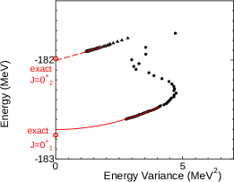
Figure 1: (Color online) Energy vs. energy variance plot of the ground state and $0^{+}_{2}$ state of ⁷²Ge by the SCG method. The circles and triangles show the energies and energy variances of $0^{+}_{1}$ and $0^{+}_{2}$, respectively. The lines are fitted for these points using a second-order polynomial.

Figure 2 shows the total energy surface provided by the $Q$-constrained Hartree-Fock calculation ringschuck using the same shell-model Hamiltonian. There are two low-energy regions corresponding to the shape coexistence phenomenon jun45 . In order to discuss the intrinsic structures of the $0^{+}_{1}$ and $0^{+}_{2}$ wave functions, we plot the deformation of each unprojected basis state $|\phi_{n}\rangle$ of the SCG wave function $|\Psi_{N}\rangle$ in Fig. 2. The location of the scattered circles shows the quadrupole deformation, namely, $\langle\phi_{n}|Q_{0}|\phi_{n}\rangle$ and $\langle\phi_{n}|Q_{2}|\phi_{n}\rangle$ where $Q_{M}$ is an $M$-component of the mass quadrupole operator and $|\phi_{n}\rangle$ is rotated so that $\langle\phi_{n}|Q_{\pm 1}|\phi_{n}\rangle=0$. It is interesting to see that the circles scatter in a broad region of the energy surface, not near the local minima, but on the hillside and triaxially deformed regions due to the effect of the configuration mixing and the “variation after projection”.

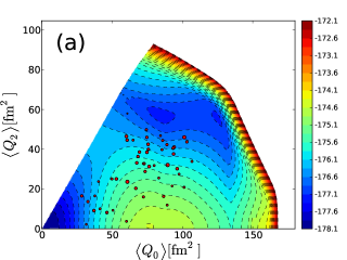
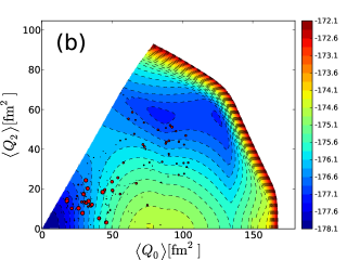
Figure 2: (Color online) Total energy surface of the ⁷²Ge by the $Q$-constrained Hartree-Fock calculation. The scattered circles denote the deformation of the basis states of the SCG wave functions for (a) $0^{+}$ ground state, and (b) second $0^{+}$ state. The contour width is 250 keV.

The area of each scattered circle on Figs. 2 (a) and (b) is proportional to the overlap probability of each projected basis state with the resulting many basis states, $\frac{1}{\cal N}|\langle\Psi_{N}|P^{J}|\phi_{n}\rangle|^{2}$, where $\cal N$ is the normalization factor, ${\cal N}=\langle\phi_{n}|P^{J}|\phi_{n}\rangle$. Concerning the $0^{+}_{1}$ state shown in Fig. 2 (a), the overlap probability is rather small and 0.54 at most. The circles with relatively large overlap scatters in a broad region of the energy surface. The overlap probability with $P^{J}|\phi_{1}\rangle$, e.g. the Hartree-Fock solution with the variation after projection is 0.32, which is modest. This overlap implies that the $0^{+}_{1}$ state is described by a linear combination of a relatively large number of basis states essentially, or the effect of the configuration mixing plays an important role. On the other hand, in Fig. 2 (b), the points of the large overlap concentrate near the spherical region concerning the $0^{+}_{2}$ state. The overlap probabilities corresponding to these points are large with the $0^{+}_{2}$ many-basis state, and the probability is 0.67 at most. This means that the wave function can be well approximated by a few number of projected Slater determinants, or mean-field description works far better than in the case of the $0^{+}_{1}$ state. This property makes the first few SCG basis states for minimizing $0^{+}_{1}$ energy dominated by the $0^{+}_{2}$ state, not by the $0^{+}_{1}$ state. These different properties of the $0^{+}_{1}$ and $0^{+}_{2}$ wave functions give rise to the different behavior of energy convergence as a function of the number of basis states, which makes extrapolation with a number of basis states difficult okinawa_shimizu .

In Fig. 1, the variance shows the local minimum at $E=-182$ MeV, which is near the energy of the $0^{+}_{2}$ state. This figure indicates that the wave function comprised of the first 10 bases are dominated by the true $0^{+}_{2}$ state, not the $0^{+}_{1}$ state. This is consistent with the discussion using the energy surface in the previous paragraph.

Such an anomalous kink in the EV plot is also seen in the $8^{+}_{1}$ state of ⁵⁶Ni with the FPD6 effective interaction fpd6 . ⁵⁶Ni is known to have shape coexistence ni_coex_mcsm , which is consistent with the previous discussion. This situation may occur in the case where the next lowest energy eigenvalue is close to the target one and the mean-field solution favors the next lowest state.

IV EVE and reordering of basis states

The emergence of the anomalous kink discussed in Sect.III gives rise to a large uncertainty of the EVE. In order to remove such a kink and to improve the precision, we introduce the reordering of basis states of the SCG wave function, represented in Eq.(1).

The SCG wave function comprises a set of $N_{m}$ basis states, $|\phi_{n}\rangle$ with $1\leq n\leq N_{m}$. These basis states also give us a sequence of approximated wave functions, $|\Psi_{N}\rangle$ with $1\leq N\leq N_{m}$, which is used for the simple EVE method. Meanwhile, reordering these $N_{m}$ basis states using a permutation, $\sigma(n)$, yields another sequence of approximated wave functions,

$$|\Psi_{N}^{\rm(ro)}\rangle=\sum_{n=1}^{N}\sum_{K=-J}^{J}f^{N{\rm(ro)}}_{n,K}P^{J\pi}_{MK}|\phi^{\rm(ro)}_{n}\rangle$$ (4)

where $|\phi^{\rm(ro)}_{n}\rangle=|\phi_{\sigma(n)}\rangle$. The corresponding energy $E^{\rm(ro)}_{N}$, and the energy variance $\langle\Delta H^{2}\rangle^{\rm(ro)}_{N}$ provide us with a new EV plot. By reordering the basis states with $\sigma(n)$, we can simulate another truncation scheme. Because the behavior of the fitted line in the EV plot depends on the truncation scheme extrap_eqs , we remove an anomalous behavior of the EV plot and make the extrapolation stable by using an appropriate $\sigma(n)$. We describe the way how to obtain an appropriate order of basis states in this section.

IV.1 Procedure of reordering technique

The relation of the energy and its variance is usually assumed to be expressed as a second-order polynomial. Because a second-order-term error is roughly estimated as $\delta c_{2}(\langle\Delta H^{2}\rangle_{N})^{2}$, where $\delta c_{2}$ is a second-order-term error of $\chi$-square fitting, the uncertainty of the second order term often causes a relatively large error of the extrapolated value in case $\langle\Delta H^{2}\rangle_{N}$, is not small enough. If we can find an order of the basis states in which the fitted curve is a first-order polynomial, the error of the extrapolation will come mainly from the coefficient of the first-order term, which can be estimated as roughly proportional to $\delta c_{1}\langle\Delta H\rangle_{N}$, where $\delta c_{1}$ is the first-order-term error of $\chi$-square fitting. This error should be far smaller than that of second-order polynomial if $\langle\Delta H^{2}\rangle_{N}$ is large. Thus, our strategy is to select the order of the basis states, in which the fitted curve is close to linear, by changing the order of the basis states.

Now, we discuss the relation between energy difference and energy variance following the idea of Ref.extrap_eqs . We define the energy difference $\delta E$ between the energy expectation value $E=\langle\Psi|H|\Psi\rangle$ of the approximated wave function $|\Psi\rangle$ and the lowest exact energy eigenvalue $E_{0}$ as

$$\delta E=\langle\Psi|H|\Psi\rangle-E_{0},$$ (5)

and the energy variance of the approximated wave function as

$$\langle\Delta H^{2}\rangle=\langle\Psi|H^{2}|\Psi\rangle-\langle\Psi|H|\Psi\rangle^{2}.$$ (6)

An approximate ground state $|\Psi\rangle$ can be decomposed into the exact eigenstate, $|\psi_{0}\rangle$, and the rest of the component, $|\psi_{r}\rangle$ as

$$|\Psi\rangle=c|\psi_{0}\rangle+d|\psi_{r}\rangle,$$ (7)

where $c^{2}+d^{2}=1$. $|\psi_{r}\rangle$ is expanded by the exact excited states such as

$$|\psi_{r}\rangle=\sum_{n\neq 0}c_{n}|\psi_{n}\rangle.$$ (8)

By defining the moments $D_{j}$ as

$$D_{j}=\sum_{n\neq 0}c_{n}^{2}(E_{n}-E_{0})^{j},$$ (9)

we obtain

$$\delta E=d^{2}D_{1},$$ (10)

$$\langle\Delta H^{2}\rangle=d^{2}D_{2}-(d^{2}D_{1})^{2}.$$ (11)

By eliminating $d^{2}$, we obtain

$$\langle\Delta H^{2}\rangle=\frac{D_{2}}{D_{1}}\delta E-(\delta E)^{2}.$$ (12)

In Eq. (11), $\langle\Delta H^{2}\rangle$ is written as a second-order polynomial of $\delta E$, which explains the parabola shape of the EV plot in Fig. 1 (circles below -182MeV). The authors of Ref.extrap_eqs solve $\delta E$ as a function of $\langle\Delta H^{2}\rangle$, which is shown to be approximated as a second-order polynomial. Now, we assume $\delta E$ is proportional to $\langle\Delta H^{2}\rangle$, which is realized in case $\frac{D_{2}}{D_{1}}\rightarrow\infty$. Because of $\frac{\partial(\delta E)}{\partial\langle\Delta H^{2}\rangle}|_{\delta E=0}=\frac{D_{1}}{D_{2}}$, we reorder the basis states so that $\frac{\partial(\delta E)}{\partial\langle\Delta H^{2}\rangle}$ is as small as possible, resulting in linear proportionality.

In practice, we perform the following procedure:

1. A fixed number, $N_{m}$, of the basis states is obtained by the SCG method.

2. Choose the $N_{m}$-th basis state $|\phi^{\rm(ro)}_{N_{m}}\rangle$ from $N_{m}$ candidates by minimizing $\frac{E^{\rm(ro)}_{N_{m}-1}-E^{\rm(ro)}_{N_{m}}}{\langle\Delta H^{2}\rangle^{\rm(ro)}_{N_{m}-1}-\langle\Delta H^{2}\rangle^{\rm(ro)}_{N_{m}}}$ .

3. Set $N$ as $N_{m}-1$. Choose the $N$-th basis state, $|\phi^{\rm(ro)}_{N}\rangle$ from $N$ candidates (basis states except for already fixed states, $|\phi^{\rm(ro)}_{N^{\prime}}\rangle$ with $N+1\leq N^{\prime}\leq N_{m}$ ) by minimizing $\frac{E^{\rm(ro)}_{N-1}-E^{\rm(ro)}_{N}}{\langle\Delta H^{2}\rangle^{\rm(ro)}_{N-1}-\langle\Delta H^{2}\rangle^{\rm(ro)}_{N}}$ .

4. Set $N$ as $N-1$. The previous step is iterated recursively up to determining the first state, $|\phi^{\rm(ro)}_{1}\rangle$.

Note that this procedure needs no additional heavy computation to the SCG, because the matrix elements of energy and its variances are evaluated once and stored, and we only require the diagonalization of the matrix whose dimension is $N\leq N_{m}\simeq 100$ for each candidate order of the basis states.

As a result, we obtain a fitted line which is closest to linear in the provided set of basis states. Because the reordering makes the gradient of the EV plot as small as possible, the anomalous kink discussed in Sect. III vanishes, which is demonstrated in the following subsection.

IV.2 ⁷²Ge in $f_{5}pg_{9}$-shell

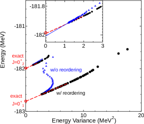
Figure 3: (Color online) Energy vs. energy variance plot for the ground state and $0^{+}_{2}$ state of ⁷²Ge in $f_{5}pg_{9}$-shell. The open triangles are obtained by the CG method without reordering and the solid circles are with reordering. The inset shows a magnified view for the $0^{+}_{2}$ energy around $\langle\Delta H^{2}\rangle\simeq 0$. See text for detail.

We apply the reordering technique to the ⁷²Ge in $f_{5}pg_{9}$-shell. The filled circles in Fig. 3 shows the EV plot with the reordering technique. The anomalous kink of the $0^{+}_{1}$ state vanishes in the plot with reordering, and the point moves smoothly and approaches the exact energy on the $y$-axis as usual mcsm_extrap . These points are fitted by a first-order polynomial, which is shown as a dashed line. Unlike the fit without reordering, these points are on the line in a large range of the energy variance which can be used for the fitting. This makes the extrapolation procedure stable.

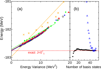
Figure 4: (Color online) (a) Energy vs. energy variance plot of the ground state energy of ⁷²Ge in the $f_{5}pg_{9}$-shell with the SCG wave function and reordering. $N_{m}=10$ (orange crosses), $20$ (green diamonds), $30$ (red triangles), $40$ (blue squares), and $50$ (open black circles). (b) Extrapolated value vs. the number of basis states, $N_{m}$. The exact energy is also shown by the dotted line. The solid points and open blue triangles denote the extrapolated energies with first-order fitting and reordering, and those with second-order fitting without reordering, respectively.

Figure 4(a) shows the EV plot provided by the SCG method with a various number of basis states, $N_{m}=10,20,30,40$ and $50$. At each $N_{m}$, the last 10 points are used to make the fitted line. While the extrapolated values of $N_{m}=10$ apparently underestimate the ground state energy, the value converges as a function of $N_{m}$ for $N_{m}\geq 30$.

Discussing the stability of the extrapolated value is difficult because all the energy-variance points with reordering change by increasing the $N$. To discuss this stability, we show the extrapolated energy itself with the reordering technique as a function of $N_{m}$. Figure 4 (b) shows the convergence property of the extrapolated energy as a function of $N_{m}$. The extrapolated energy with reordering using the last 10 points, or $(N_{m}-9)$-th, $(N_{m}-8)$-th, … $N_{m}$-th points, converges well within a few keV for $N_{m}>40$. On the other hand, the extrapolated value without reordering shows a large fluctuation due to the kink in the EV plot.

The inset of Fig. 3 shows the EV plot concerning $J=0^{+}_{2}$. The open triangles and the fitted line show the energy and variance without reordering. Its extrapolation underestimates 20 keV, the exact value, while the extrapolated value with the reordering technique agrees with the exact one within the 6 keV error. The reordering technique reduces the error of the extrapolation even in the case of the simple EVE without reordering, and works well.

IV.3 ⁶⁴Ge in $pfg9$-shell

In Ref. mcsm_extrap , we show a demonstration of the validity of the MCSM and energy-variance by ⁶⁴Ge in the $pf+g_{9/2}$-shell model space, which consists of $0f_{7/2},0f_{5/2},1p_{3/2},1p_{1/2}$ and $0g_{9/2}$ single-particle orbits. We use the PFG9B3 effective interaction pfg9b3 , which was also used in Refs. horoi_leveldens ; mcsm_extrap . The $m$-scheme dimension of the system reaches $1.7\times 10^{14}$, which cannot be reached by the conventional Lanczos diagonalization technique. In the present work, this nucleus is taken as an example again. We show the results using the SCG method and by extrapolation with the reordering technique in Fig. 5. As you can see, the extrapolated energies with reordering technique well converge in a relatively small number of basis states. In this case, the energies with reordering agree well with those without reordering, and those of the MCSM method which are shown in Ref.mcsm_extrap .

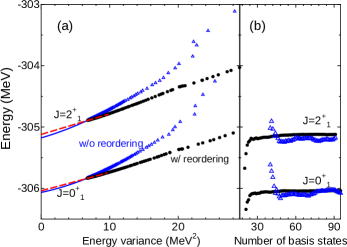
Figure 5: (Color online) (a) Energy vs. energy variance plot for the $0^{+}_{1}$ and $2^{+}_{1}$ states of ⁶⁴Ge in the $pfg9$-shell obtained by the SCG method. (b) Extrapolated energies with reordering (filled circles) and without reordering (open triangles) as functions of $N_{m}$.

V Summary

We have discussed variational procedures, the SCG method, for nuclear shell-model calculations. Based on the SCG wave functions, we propose a new procedure of energy variance extrapolation, which can solve a complex problem due to shape coexistence.

For example, the simple EVE is difficult to solve at the $0^{+}_{1}$ state of ⁷²Ge with the JUN45 interaction. In this case, the anomalous kink appears in the EV plot, which shows the transition of the approximated wave function from the second lowest state to the lowest state. We discussed its origin in view of shape coexistence, and found that the reordering technique of the basis states allows us to extrapolate the eigenenergy successfully even in this case.

We demonstrated that the reordering technique in the EV plot allows us to make a linear fit; and therefore, the reordering of the basis states makes the extrapolation procedure stable and suppresses the uncertainties of the extrapolated value. This procedure is expected to be quite useful into performing the precise estimate of nuclear energies based on large-scale shell-model calculations and no-core shell-model calculations okinawa_tabe . For the estimatation of observables other than energy, such as quadrupole moment, the order which was used in the present work is not suitable for the extrapolation procedure. We are investigating a way to determine an order suitable for the extrapolation of these observables.

- (1) M. Honma, T. Mizusaki, and T. Otsuka, Phys. Rev. Lett. 75, 1284 (1995).
- (2) T. Otsuka, M. Honma, T. Mizusaki, N. Shimizu, and Y. Utsuno, Prog. Part. Nucl. Phys. 47, 319 (2001).
- (3) M. Honma, B. A. Brown, T. Mizusaki, and T. Otsuka, Nucl. Phys. A 704, 134c (2002), M. Honma, T. Otsuka, B.A. Brown and T. Mizusaki, Phys. Rev. C 65, 061301(R) (2002).
- (4) K. W. Schmid, Prog. Part. Nucl. Phys. 52, 565 (2004).
- (5) S. Pittel and N. Sandulescu, Phys. Rev. C 73, 014301 (2006).
- (6) G. Puddu, J. of Phys. G: Nucl. Part. Phys. 32 321 (2006), G. Puddu, Eur. Phys. J. A 34, 413 (2007).
- (7) R. Roth, and P. Navratil, Phys. Rev. Lett. 99 092501 (2007)
- (8) Z.-C. Gao, M. Horoi, and Y. S. Chen, Phys. Rev. C 80, 034325 (2009)
- (9) M. Horoi, A. Volya, and V. Zelevinsky, Phys. Rev. Lett. 82, 2064 (1999); M. Horoi, B. A. Brown, and V. Zelevinsky, Phys. Rev. C 67 034303 (2003).
- (10) T. Papenbrock and D. J. Dean, Phys. Rev. C 67, 051303(R) (2003).
- (11) J.J. Shen, Y. M. Zhao, A. Arima, and N. Yoshinaga, Phys. Rev. C 83, 044322 (2011).
- (12) T. Mizusaki and M. Imada, Phys. Rev. C 65, 064319 (2002).
- (13) T. Mizusaki and M. Imada, Phys. Rev. C 67, 041301 (2003).
- (14) T. Mizusaki and N. Shimizu, Phys. Rev. C 85, 021301(R) (2012).
- (15) T. Mizusaki, Phys. Rev. C 70, 044316 (2004).
- (16) H. Zhan, A. Nogga, B.R. Barrett, J.P. Vary and P. Navratil, Phys. Rev. C 69, 034302 (2004).
- (17) N. Shimizu, Y. Utsuno, T. Mizusaki, T. Otsuka, T. Abe, and M. Honma, Phys. Rev. C 82, 061305(R) (2010).
- (18) M. Imada and T. Kashima, J. Phys. Soc. Jpn. 69 2723 (2000).
- (19) N. Shimizu, Y. Utsuno, T. Mizusaki, T. Otsuka, T. Abe and M. Honma, AIP Conf. Proc. 1355, 138 (2011).
- (20) Numerical Recipes in Fortran 77, the Art of Scientific Computing, 2nd ed., Cambridge University Press: Cambridge, (1992).
- (21) T. Abe, P. Maris, T. Otsuka, N. Shimizu, Y. Utsuno, and J. P. Vary, AIP Conf. Proc. 1355, 138 (2011).
- (22) M. Honma, T. Otsuka, T. Mizusaki, and M. Hjorth-Jensen, Phys. Rev. C 80, 064323 (2009).
- (23) T. Mizusaki, N. Shimizu, Y. Utsuno, and M. Honma, code MSHELL64, unpublished.
- (24) P. Ring and P. Schuck, The Nuclear Many-Body Problem, Springer-Verlag, New York, 1980.
- (25) W.A. Richter, M.G. van der Merwe, R.E. Julies and B.A. Brown, Nucl. Phys. A523, 325, (1991).
- (26) T. Mizusaki, T. Otsuka, Y. Utsuno, M. Honma and T. Sebe, Phys. Rev. C 59 R1846 (1999).
- (27) M. Honma et al., unpublished.
- (28) R. A. Sen’kov and M. Horoi, Phys. Rev. C 82 024304 (2010).