Thawing Versus. Tracker Behaviour: Observational Evidence
Abstract
Currently there are a variety of scalar field models that attempt to explain the late time acceleration of the Universe. This includes the standard canonical and non-canonical scalar field models together with recently proposed Galileon scalar field models. One can divide all these scalar field models into two broad categories, namely the thawing and the tracker classes. In this work we investigate the evidence for these models with the presently available observational data using the Bayesian approach. We use the Generalized Chaplygin Gas (GCG) parametrization for dark energy equation of state (EoS) as it exhibits both the thawer and tracker like behaviours for different values of the parameters. Subsequently we use the SnIa ( SN) measurements, the recent measurements of the Hubble parameter at different redshifts (H(z)), measurements of the lookback time at different redshifts (Lookback), measurements of the linear growth factor in large scale structure (GR) from various redshift surveys and finally the measurement of the anisotropies in the cosmic microwave background radiation by WMAP-7 observations. The analysis of data from SN+H(Z)+Lookback does not favour either the tracker or thawer classes. Inclusion of data from GR+WMAP-7 favours the thawer class of models if one assumes the dark energy to be a smooth component. But if we consider the dark energy perturbation, both tracker and thawer type of models are equally favoured by the data.
keywords:
Cosmology:Dark Energy, scalar fields, GCG, WMAP, SnIa .1 Introduction
It is now firmly established that the present Universe is going through a phase of accelerated expansion. This has been confirmed by different observational results including Type-Ia supernovae ( Riess et al. (1998), Perlmutter et al. (1999), Tonry et al. (2003), Knop et al. (2003), Riess et al.(2004), Amanullah et al. (2010), Suzuki et al. (2011)), cosmic microwave background radiation ( Komatsu et al. (2011)) as well as the latest surveys of the large scale structue ( Eisenstein et al. (2005)). The challenge is now to explain the possible cause for this late time acceleration and there has been a wide range of proposals for this. One of the possible sources for this accelerated expansion could be an exotic type of matter with an equation of state parameter . Such sources are collectively called Dark Energy. [see ( Bean et al. (2005), Copeland et al. (2006), Li et al. (2011), Padmanabhan(2003), Peebles & Ratra (2003), Sahni & Starobinsky (2000)) for review on dark energy models].
The simplest example for this dark energy is a cosmological constant (CC) , but the need for an extreme fine tuning and the cosmic coincidence problem make an unattractive choice from a theoretical perspective. The scalar field models are a natural alternative. Different scalar field models including quintessence ( Ratra & Peebles (1988), Caldwell et al. (1998), Liddle & Scherrer (1999), Steinhardt et al. (1999)), tachyon ( Abramo & Finelli (2003), Bagla et al. (2003), Aguirregabiria & Lazkoz (2004), Copeland et al. (2005)), phantom ( Caldwell (2002)) and k-essence ( Armendariz et al. (2001), Scherrer (2004), Sen (2006), Vikman (2005)) as well as Galileons ( Nicolis et al. (2009), Ali et al. (2010), Gannouji & Sami (2010), Appleby & Linder (2011), Linder (2012), De. Felice & Tsujikawa (2010)) have been thoroughly investigated in recent time to explain the late time acceleration of the Universe. In addition to circumvent the problem like cosmic coincidence, the advantage of using these fields is that they also mimic CC at late times. Moreover, as the equation of state (EoS) for these scalar fields in general vary with time, it is expected that these scalar field models can be distinguished from CDM with observational data from higher redshifts which are expected to become available in near future.
Scalar field models in general, can be divided into two broad classes: the fast roll and slow roll models, also termed as tracking and thawing models, respectively ( Caldwell & Linder (2005), Linder (2003)). Tracker models with steep potentials usually mimic the background matter/radiation in the early time and remains subdominant. Only at late times, the field leaves the tracker regime and starts behaving like a component with large negative pressure and thereby behaves like dark energy. On the other hand, thawing models are similar to inflaton, where the scalar field is initially frozen due to the large Hubble friction in the flat part of the potential and hence behaves close to CC. At late times, the scalar field slowly thaws from this frozen state and departs from this CC behaviour. In both these cases, a certain degree of fine tuning (whether in the form of the potentials or in the initial conditions) is always necessary to get the required late time evolution.
With the high level of precision that exists in current observational techniques, the question naturally arises as to whether the available observational data indicate any clear preference of one of these models over the other. In the present exercise, we attempt to answer this question using the Bayesian approach. To do so, it is important to look for a parametrization for the dark energy behaviour which interpolates between the tracker and the thawer behaviour. It has been however pointed out that general barotropic models described by can not fully mimic the scalar field models and in particular the tracker type of models ( Scherrer (2006), Linder & Scherrer (2009)). However, the attempt in this paper is to have a single model that broadly mimics the two overall behaviours, namely: 1) the equation of state is frozen initially at and then at late times it slowly thaws out from this frozen state which is similar to thawer type of scalar fields and 2) the equation of state is that of matter initially and later on starts behaving like cosmological constant which is similar to tracker type of scalar fields. Fortunately a widely studied form, known as ”Generalized Chaplygin Gas” (GCG) ( Kamenshchik et.al. (2001), Bento et al. (2002), Sen & Scherrer (2005)), can provide such a parametrization scheme [ See also ( Aviles & Cervantes-Cota (2011))]. This single parametrization for the EoS of the dark energy can not only mimic both of these two behaviours, it can also act as dark energy with constant EoS (including which is the same as CC). Using this parametrization we show that considering only the homogenous background cosmology and applying it to analyze observational data does not discriminate between thawing and tracker type of behaviours. However, if we include the data from the growth of matter perturbations as well as those from CMBR anisotropies, thawing type models are preferred if we do not consider the perturbation in the GCG fluid. But including perturbations in the GCG fluid results no preference of thawer over tracker type of behaviour.
2 GCG
We start by discussing the equation of state for GCG given by,
| (1) |
where and are two arbitrary constants ( Bento et al. (2002)). Assuming Friedmann-Robertson-Walker metric, this equation of state implies that the density evolves with redshift as
| (2) |
where
| (3) |
with being the present value of . The choice of the constants, and uniquely determines the dark energy behaviour in the GCG model.
One can easily show that . As our primary goal is to compare the thawing and tracking behaviours which primarily arise in the scalar field models, we confine ourselves to non-phantom region i.e . For , GCG exactly behaves as CC at all times and in this case the parameter is redundant. For , GCG behaves exactly as a non-relativistic pressureless matter fluid at all times.
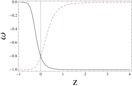
For , the parameter determines the how the equation of state changes with time. For , the GCG behaves as a fluid with constant equation state . For , at early times GCG behaves as matter while at late times it behaves as a fluid with negative equation of state and asymptotically tends to a Cosmological Constant like behaviour in the future. This is exactly what we need for a tracking behaviour. On the other hand, for , GCG behaves as a cosmological constant to start with and then as the Universe evolves, it starts deviating from this CC behaviour ( Sen & Scherrer (2005)). This is similar to the thawing behaviour. Further, in this case, GCG always approaches to matter behaviour assymptotically in the future (). Hence, in this model, accelerated expansion is a transient feature. All these different behaviours are shown in Figure 1.
To summarise, GCG behaves as a tracking model for whereas it behaves as thawing model for . For , GCG behaves as a fluid with a constant equation of state
| (4) |
It demarcates the thawing from the tracking regime.
 |
 |
 |
 |
Considering the fact that GCG can effectively represent both the thawing as well as the tracking behaviour by suitable parametrization, we use this feature to discriminate between these two models on the basis of Bayesian analysis using the current observational data.
3 Data
We consider the Supernovae Type Ia observation which is a direct probe for the cosmic expansion. These observations measure the apparent luminosity of the Supernovae as observed by an observer on earth. It is related to the luminosity distance defined as
| (5) |
Using this, we evaluate the distance modulus (which is an observable quantity) as
| (6) |
where m and M are, respectively, the apparent and absolute magnitudes of the Supernovae. We consider the latest Union2.1 data compilation ( Suzuki et al. (2011)) consisting of 580 data points for the observable .
We also use determinations of the cosmic expansion history from red-envelope galaxies by Stern et al. ( Stern et al. (2010)). They have obtained a high-quality spectra of red-envelope galaxies in 24 galaxy clusters in the redshift range using the Keck-LRIS spectrograph. Subsequently they have complemented these with high-quality, archival spectra as obtained by the SPICES and VVDS surveys. With this, we get 12 measurements of the Hubble parameter H(z) at different redshifts. The measurement of the Hubble parameter at present (i.e. ) is obtained from the HST Key project.
The observational data of SNe Ia and Hubble(H(z)), mentioned above relies on the measurements of cosmological distances at certain redshifts. On the other hand, the lookback time to high redshift objects, as proposed by ( Dalal et al. (2001)) depends on the measurement of age of the Universe at a particular redshift. The test based on the lookback time when combined with the distance measurements can be very useful to constrain cosmological models.
Lookback time is defined as the difference between the present age of the Universe and its age at redshift z, and is given by ( Cappzziello et al. (2004))
| (7) | |||
| (8) |
where represents the set of model parameters, and .
The observed lookback time of an object at redshift is defined as
| (9) |
where is the observed age of the Universe. We use the value of billion years for ( MacTavish et al (2005)). The incubation time has been denoted by and it is different for different objects. It is taken to be a nuisance parameter in our study and we marginalize over this parameter ( Dantes et al. (2007)). The data for lookback time is obtained from ( Simon et al. (2005)).
 |
 |
 |
 |
We further use the measurement of CMB anisotropy by WMAP-7 observations ( Komatsu et al. (2011)). Using the publicly available code CAMB ( Lewis et al. (2000)), we calculate the expected CMB anisotrpy spectrum for GCG as a function of its two model parameters and and the cosmological parameter . To incorporate the dark energy perturbation, we use publicly available PPF Module for CAMB ( Fang et al (2008a), Fang et al. (2008b)). In this case, GCG fluid is used as a dark energy with equation of state given in eqn (4) and the speed of sound as this fluid represents a parametrization of the scalar field models ( For detail calculation and relevant equations in PPF module, see ( Fang et al. (2008b))).
The other cosmological parameters are equated to their best fit values as derived from the data from WMAP-7. We compare our theoretical results with the data and do the likelihood analysis using the likelihood code provided by the WMAP team ( Komatsu et al. (2011) ).
The growth of large scale structures is another useful observational probe to distinguish between different dark energy models. The growth rate of large scale structures is calculated from matter density perturbation in the linear regime and subhorizon scales . On these scales where one measures the growth, one can safely ignore the dark energy perturbations as it only affects the fluctuations comparable to Hubble scales. The effect of dark energy is only through the background expansion and one can use the Newtonian limit for the evolution of the matter density fluctuation satisfying the equation:
| (10) |
The growth factor is related to the linear density contrast by . The compilation of data for growth factor measurements from different redshift surveys can be found in ( Gupta et al. (2011)) ( See also references therein).
4 Results
Using observational data mentioned above we calculate the joint likelihood for the GCG model as:
| (11) |
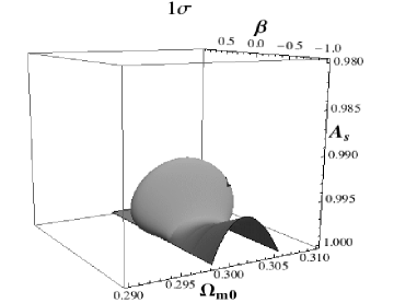
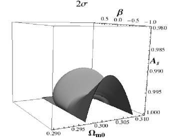
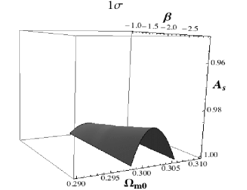
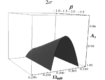
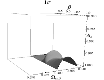
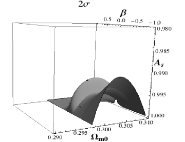
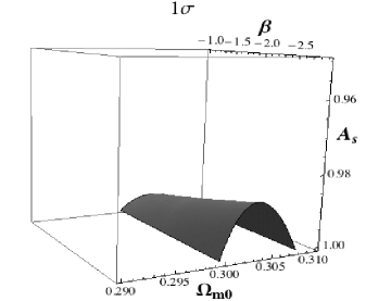
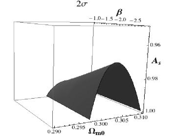
Before calculating the Bayesian Evidence for thawing type and tracker type of models, we maximise the likelihood function and calculate the allowed region in the parameter space of and for both thawing type and tracking type of models. The results are shown in Figure (2) and Figure (3). In these figures we show the 3-D contours in the region. For the tracker type of models ( shown in Figure (2 and 3)), it is clear that upto confidence level, the allowed behaviours are extremely close to C.C. This is apparent from the bound on which varies negligibly from , behaviour. The constraint on parameter is also extremely tight, . Also, in this case, all the values of are allowed. But for two specific values of , the allowed value of is maximum. These are for which GCG behaves as a DE with constant equation of state and for for which GCG itself behaves as a combination of and matter fluid. For only is allowed which is similar to C.C.
For thawing case ( shown in Figure (2 and 3)), the variation of parameter is marginally higher than the tracking case, but here also the constraint on is extremely tight. Also in this case, all values of are allowed, but as one increases , the allowed values for get decreased.
To summarise, with all the data, the GCG parametrization puts extremely tight constraint on the dark energy behaviour and the cosmological parameter .
We now proceed to substantiate this conclusion. In order to do this we calculate the Bayesian Evidence for both the thawing as well as tracking behaviour. This is defined as ( Liddle et al. (2006))
| (12) |
where represents the set of model parameters, represents the Likelihood function and is the prior probability distribution for parameter . In our case, we have three parameters and . As we have no prior knowledge about these parameters, we assume uniform prior for these three parameters.We get a thawing behaviour for and tracking for . For the thawing case we assume that is uniformly distributed in the range while for tracking case we assume that is uniformly distributed in the range . fixes the equation of state for dark energy at present () and we assume that it is uniformly distributed between and for both thawing as well as tracking case. We also assume that for both the cases, is uniformly distributed between and .
According to Jeffrey’s interpretation ( Jeffreys(1998)), if between and , it is a significant evidence for a model with higher while the same between and is a strong to very strong evidence. If is more than , the model with higher is decisively favoured.
We calculate assuming thawing () and tracking () as two different models. We get the following results:
| (13) |
| (14) |
with D.E. perturbation
| (15) |
without D.E. perturbation
From these results, it is clear that although observational data from the smooth background cosmology cannot discriminate between thawing and tracking behaviour, when these are complemented with the information from the inhomogenous universe but assuming uniform dark energy distribution there is significant evidence in favour of thawing behaviour ( with odds ratio 5:1). However, when we take into account the perturbation in the dark energy component while calculating the CMBR spectra, this preference over thawing type of models is lost and there is no Bayesian evidence to prefere any type of behaviours.
We should also mention that although we choose a specific prior for and as mentioned above, the results are only weakly sensitive to these priors. In order to verify this we have varied these priors and we found that the above results remain almost the same. This makes our result sufficiently robust.
5 Discussion and Conclusions
Several observed features of the Universe depend on the precise nature of cosmological expansion. Broadly the evolution of Universe with a dark energy can be classified in two categories. In one case the DE equation of state is frozen at the in the early universe due to large Hubble friction but in the late time as the Hubble friction eases out, the equation of state slowly thaws out of this frozen state. This is so called thawing behaviour and can be modelled by the scalar field with slow-roll potentials. In the other case, the DE equation equation of state mimics the background matter in the early universe and in the late time it starts behaving like a C.C. This type of behaviour is called tracker type and can be mimicked by the scalar fields with steeper potentials. Here we parametrize these two overall behaviours by the GCG type of equation of state and investigate whether the observational data prefer any one of them.
Towards this end we have first used data pertaining to the background cosmology. In particular, we have considered three types of data: (i) Supernova Type 1A, (ii) Hubble parameter evolution with redshift, and (iii) Lookback time of Galaxies. For the Supernova Data we have used the Union2.1 data. The data from Keck-LRIS, SPICE and VVDS has been used for the evolution of hubble parameter while for the present redshift hubble parameter HST Key project has been used. For the look back time calculation, the incubation time of the galaxies has been marginalized over as we do not have definitive information about it.
We have then complemented these with the information from inhomogeneous universe. For this we have used the results of CMB Anisotropy (as given in the WMAP-7 data) and the growth of large-scale structures.
Our results indicate that if we take into account only the smooth background cosmology, then the data is insufficient to give a clear verdict either way. On the other hand, if we complement this with the information from inhomogeneities in the Universe then there seems to be a preference for the thawing model if one does not consider the dark energy perturbations while calculating the CMBR spectra. In terms of Bayesian evidence, this preference for thawing behaviour is significant. However, we find that incorporating the dark energy perturbation to calculate the CMBR spectra, this preferance for thawing type of behaviour is lost.
We stress that the GCG cannot represent the full scalar field dynamics for tracker type of models in particular and this weakens our conclusion. Nevertheless, our analysis is the first one to investigate whether observational data prefer a thawing or tracking type of behaviour.
6 Acknowledgement
A.A.S. and T.R.S. acknoweldge the financial support provided by C.S.I.R. Govt. of India through the research grant (Grant No:03(1187)/11/EMR-II). S.T is fully funded by C.S.I.R. Govt. of India. S.T. and T.R.S. acknowledge facilities provided by Inter University for Astronomy and Astrophysics, Pune, India through IUCAA Resource Centre (IRC) at Department of Physics and Astrophysics, University of Delhi, New Delhi, India. S.T. acknowledges the computational facilities provided by the CTP, JMI, New Delhi, India. Part of the numerical computations were performed using the Cluster computing facility at the Harish-Chandra Research Institute,Allahabad, India (http://cluster.hri.res.in/index.html).
We thank the LAMBDA project for providing the data and likelihood code for WMAP7 (http://lambda.gsfc.nasa.gov/product/map/current/). We thank A. Lewis and A. Challinor for the publicly available CAMB code. We also thank W. Fang for the publicly available PPF module for CAMB.
References
- Abramo & Finelli (2003) Abramo L.R.W.,& Finelli F.,2003, Phys.Lett.B, 575,165
- Aguirregabiria & Lazkoz (2004) Aguirregabiria J.M. & Lazkoz R., 2004, Phys.Rev.D, 69, 123502
- Ali et al. (2010) Ali A., Gannouji R., Sami M., 2010, Phys.Rev.D 82, 103015
- Amanullah et al. (2010) Amanullah R., et al., 2010, ApJ 716, 712
- Appleby & Linder (2011) Appleby S.A., Linder E., 2011, arXiv:1112.1981
- Armendariz et al. (2001) Armendariz-Picon C., Mukhanov V. & Steinhardt P.J., 2001, Phys.Rev.D 63, 103510
- Aviles & Cervatnes-cota (2011) Aviles A & Cervantes-Cota J. L, 2011, Phys. Rev. D 84, 083515
- Bagla et al. (2003) Bagla J.S, Jassal H.K & Padmanabhan T., 2003, Phys. Rev.D 67, 063504
- Bean et al. (2005) Bean R., Carroll S. & Trodden M., 2005, arXiv:astro-ph/0510059
- Bento et al. (2002) Bento M.C., et al., 2002, Phys. Rev. D 66, 043507
- Caldwell et al. (1998) Caldwell R. R., Dave R. & Steinhardt P. J., 1998, Phys. Rev. Lett. 80, 1582
- Caldwell (2002) Caldwell R.R., 2002, Phys. Lett. B 545, 23
- Caldwell & Linder (2005) Caldwell R. R. & Linder E. V., 2005, Phys. Rev. Lett. 95, 141301
- Cappoziello et al. (2009) Cappoziello S. et al., 2004, Phys. Rev. D 70, 123501
- Copeland et al. (2005) Copeland E.J, Garousi M.R , Sami M. & Tsujikawa S., 2005, Phys. Rev. D 71, 043003
- Copeland et al. (2006) Copeland E.J., Sami M.& Tsujikawa S., 2006, Int. J. Mod. Phys. D 15, 1753
- Dalal et al. (2001) Dalal N., Abazajian K., Jenkins E. & Manohar A.V., 2001, Phys. Rev. Lett. 87, 141302
- Dantes et al. (2007) Dantes M.A., Alcaniz J.S., Jain D. & Dev A. 2007, Astron. Astrophysics 467, 421
- De. Felice & Tsujikawa (2010) De.Felice A, & Tsujikawa, S., 2010 Phys. Rev. Lett. 105, 111301
- Eisenstein et al. (2005) Eisenstein D.J. et al., 2005, Astrophys.J. 633, 560
- Fang et al. (2008a) Fang W., Hu W. & Lewis A., 2008a, Phys. Rev. D 78, 087303
- Fang et al. (2008b) Fang W. et al., 2008b, Phys. Rev. D 78, 103509; http://camb.info/ppf.
- Gannouji & Sami (2010) Gannouji R. & Sami M., 2010, Phys. Rev. D 82, 024011
- Gupta (2011) Gupta Gaveshna, Sen Somasri & Sen Anjan.A., 2011, arxiv:1110.0956 [astro.ph]
- Jeffreys (1998) Jeffreys H.,1998, Theory of Probablity, 3rd Edition [OUP, Oxford]
- Kamenshchik et al. (2001) Kamenshchik A. Y, Moschella U. & Pasquier V. 2001, Phys. Lett. B 511, 265
- Knop et al. (2003) Knop R. A., et al., 2003, Astrophys.J. 598, 102
- Komatsu et al. (2011) Komatsu E., et al., 2011, Astrophys. J. Suppl. 192, 18
- Lewis et al. (2011) Lewis A.,Challinor A.& Lasenby A.,2000, Astrophys. J. 538, 473.; http://camb.info
- Li et al. (2011) Li M., Li X.D. & Wang S., 2011, arXiv:1103.5870 [astro-ph,CO]
- Liddle et al. (2006) Liddle A.R., Mukherjee P. & Parkinson D., 2006, Astron. Geophys. 47, 4.30
- Liddle & Scherrer (1999) Liddle A. R. & Scherrer R. J, 1999, Phys. Rev. D, 59, 023509
- Linder (2003) Linder E.V., 2003, Phys. Rev. Lett. 90, 091301
- Linder (2012) Linder E., 2012, arXiv:1201.5127
- Linder & Scherrer (2009) Linder E. & R. J. Scherrer, 2009, Phys. Rev. D, 80 023008
- MacTavish (2005) MacTavish C.J. et al. 2005 astro-ph/0507503
- Nicolis et al. (2009) Nicolis A., Rattazzi R. & Trincherini E., 2009, Phys. Rev. D 79, 064036
- Padmanabhan (2003) Padmanabhan T., 2003, Phys.Rep. 380, 235
- Peebles & Ratra (2003) Peebles P.J.E. & Ratra B., 2003, Rev. Mod. Phys. 75, 554
- Perlmutter et al. (1999) Perlmutter S. et al., 1999, Astrophys.J. 517, 565
- Ratra & Peebles (1988) Ratra B. & Peebles P.J.E., 1988, Phys. Rev. D 37, 3406
- Riess et al. (1998) Riess A. G., et al., 1998, Astron. J. 116, 1103
- Riess et al. (2004) Riess A.G., et al., 2004, Astrophys. J. 607, 665
- Sahni & Starobinsky (2000) Sahni V. & Starobinsky A., 2000, Int. J. Mod. Phys. D 9, 373
- Scherrer (2004) Scherrer R.J., 2004, Phys.Rev.Lett 93, 011301
- Scherrer (2006) Scherrer R.J., 2006, Phys. Rev. D, 73, 043502
- Sen (2006) Sen A.A., 2006, JCAP 0603:010
- Sen & Scherrer (2005) Sen A.A. & Scherrer R.J., 2005, Phys. Rev. D 72, 063511
- Simon et al (2005) Simon J., Verde L. & Jimenez R., 2005 Phys.Rev.D 71, 123001
- Steinhardt et al. (1999) Steinhardt P. J., Wang L. & Zlatev I., 1999, Phys. Rev. D, 59, 123504
- Stern et al. (2010) Stern D. et al., 2010, JCAP 1002, 008
- Suzuki et al. (2011) Suzuki N., et al., 2011, arXiv:1105.3470
- Tonry et al. (2003) Tonry J.L., et al., 2003, Astrophys.J. 594, 1
- Vikman (2005) Vikman A., 2005, Phys.Rev.D 71, 023515