Stability analysis for pitchfork bifurcations of solitary waves in generalized nonlinear Schrödinger equations

Abstract

Linear stability of both sign-definite (positive) and sign-indefinite solitary waves near pitchfork bifurcations is analyzed for the generalized nonlinear Schrödinger equations with arbitrary forms of nonlinearity and external potentials in arbitrary spatial dimensions. Bifurcations of linear-stability eigenvalues associated with pitchfork bifurcations are analytically calculated. It is shown that the smooth solution branch switches stability at the bifurcation point. In addition, the two bifurcated solution branches and the smooth branch have the opposite (same) stability when their power slopes have the same (opposite) sign. One unusual feature on the stability of these pitchfork bifurcations is that the smooth and bifurcated solution branches can be both stable or both unstable, which contrasts such bifurcations in finite-dimensional dynamical systems where the smooth and bifurcated branches generally have opposite stability. For the special case of positive solitary waves, stronger and more explicit stability results are also obtained. It is shown that for positive solitary waves, their linear stability near a bifurcation point can be read off directly from their power diagram. Lastly, various numerical examples are presented, and the numerical results confirm the analytical predictions both qualitatively and quantitatively.

1 Introduction

Bifurcation of solitary waves is an important phenomenon in nonlinear wave equations. One type of bifurcation is the so-called pitchfork bifurcation, where a smooth branch of solitary waves exists on both sides of the bifurcation point, but two additional solution branches bifurcate out to only one side of the bifurcation point. The most common pitchfork bifurcation of solitary waves is the symmetry-breaking bifurcation, where solitary waves on the smooth branch have certain symmetry, but solitary waves on the bifurcated branches lose that symmetry and become asymmetric. This symmetry-breaking bifurcation occurs frequently in various nonlinear wave models originating from diverse physical disciplines (such as nonlinear optics and Bose-Einstein condensates). For instance, this bifurcation has been reported in the nonlinear Schrödinger (NLS) equations with external potentials [2, 3, 4, 5, 6, 7, 8, 9, 10, 11, 12]. Physically these NLS equations govern nonlinear light propagation in refractive-index-modulated optical media [13, 14] and atomic interaction in Bose-Einstein condensates loaded in magnetic or optical traps (in the latter community these equations are called the Gross-Pitaevskii equations [15]). This symmetry-breaking bifurcation has also been reported in the linearly-coupled NLS equations which govern light transmission in dual-core couplers [16, 17]. Analytical studies of symmetry-breaking bifurcations have also been made, mostly for the NLS equations with special types of nonlinearities and potentials (see [2, 5, 7, 9, 10, 12] for instance). In [2] the authors considered a one-dimensional NLS equation with focusing cubic nonlinearity and a Dirac-type symmetric double-well potential, and showed the presence of symmetry breaking bifurcation as well as the exchange of dynamical stability from the symmetric branch to the asymmetric branch at the bifurcation point. In [5] the authors considered a class of multi-dimensional NLS equations with focusing cubic nonlinearity and symmetric potentials, and showed that symmetry-breaking bifurcation occurs when the power (also called the squared norm in mathematics and particle numbers in Bose-Einstein condensation) of the symmetric solitary waves increases above a certain threshold, provided that the first two eigenvalues of the linear potential are sufficiently close to each other (such as in double-well potentials with large separation between the two wells). In addition, the authors showed that above this power threshold, the symmetric states become unstable, and a pair of orbitally stable asymmetric states appear. In [7], the author considered a class of multi-dimensional NLS equations with defocusing power nonlinearity and symmetric double-well potentials in the semiclassical limit, and showed that symmetry-breaking bifurcations occur for antisymmetric solitary waves. In [9], the authors considered a class of one-dimensional NLS equations with focusing power nonlinearity and a symmetric potential, and showed that symmetry-breaking bifurcation occurs for positive symmetric solitary waves if the potential satisfies certain requirements. In addition, they showed that the symmetric branch changes stability at the bifurcation point, and the asymmetric branches can be orbitally stable or unstable under different conditions. In [10], the authors considered the same class of equations as in [9] and obtained normal forms for these symmetry-breaking bifurcations. In [12], this author considered the general class of NLS equations with arbitrary forms of nonlinearities and potentials in arbitrary spatial dimensions, and derived the general analytical conditions for pitchfork bifurcations as well as the power formulae for solitary-wave branches near the pitchfork bifurcation point.

In this paper, we consider the general nonlinear Schrödinger equations with arbitrary forms of nonlinearity and potentials in arbitrary spatial dimensions (as in [12]). These equations include the Gross-Pitaevskii equations in Bose-Einstein condensates with attractive or repulsive atomic interactions and nonlinear light-transmission equations in linear potentials or nonlinear lattices with power or non-power nonlinearities as special cases [13, 14, 15, 18]. For this large class of equations, we determine the linear stability of both sign-definite (positive) and sign-indefinite solitary waves near pitchfork bifurcations. Our strategy is to explicitly calculate the bifurcation of linear-stability eigenvalues from the origin, which always takes place whenever a pitchfork bifurcation occurs (see Theorem 3 in Sec. 3). Based on this eigenvalue bifurcation and assuming no other instabilities interfere, linear stability of solitary waves near pitchfork bifurcations is then obtained (see Theorem 4 in Sec. 3). We show that the smooth solution branch always switches stability at the bifurcation point. In addition, the bifurcated solution branches and the smooth branch have opposite (same) stability when their power slopes have the same (opposite) sign. One unusual feature on the linear stability of these pitchfork bifurcations is that the smooth and bifurcated solution branches (on the same side of the bifurcation point) can be both stable or both unstable, which contrasts such bifurcations in finite-dimensional dynamical systems where the smooth and bifurcated branches generally have opposite stability [19]. For the special case of positive solitary waves, stronger and more explicit stability results are also obtained (see Theorem 5 in Sec. 3). We show that for positive solitary waves, their linear stability near a pitchfork bifurcation point can be read off directly from their power diagram. Specifically, their linear stability is simply determined by which side of the bifurcation point the bifurcated solutions appear and whose power slope of the smooth and bifurcated solutions is larger. Lastly, we present various numerical examples, and show that the numerical results confirm the analytical predictions both qualitatively and quantitatively.

Compared with the earlier analytical results on stability of pitchfork bifurcations (such as in [2, 5, 7, 9]), our stability results have the following three distinctive features. First, our results apply to the general NLS equations with no restriction on the nonlinearity, potential or spatial dimensions. Second, we made a direct link between linear stability and the power diagram (especially for positive solitary waves whose linear stability can be read off entirely from the power diagram). Third, we derived explicit analytical formulae for linear-stability eigenvalues of solitary waves, which can be useful when quantitative prediction of linear instability is needed.

2 Preliminaries

We consider the generalized nonlinear Schrödinger (GNLS) equations with arbitrary forms of nonlinearity and external potentials in arbitrary spatial dimensions. These equations can be written as

$$iU_{t}+\nabla^{2}U+F(|U|^{2},\mathbf{x})\hskip 1.70709ptU=0,$$ (2.1)

where $\nabla^{2}=\partial^{2}/\partial x_{1}^{2}+\partial^{2}/\partial x_{2}^{2}+\cdots+\partial^{2}/\partial x_{N}^{2}$ is the Laplacian in the $N$-dimensional space $\textbf{x}=(x_{1},x_{2},\cdots,x_{N})$, and $F(\cdot,\cdot)$ is a general real-valued function which includes nonlinearity as well as external potentials. These GNLS equations include the Gross-Pitaevskii equations in Bose-Einstein condensates [15] and nonlinear light-transmission equations in linear potentials and nonlinear lattices [13, 14, 18] as special cases. Notice that these equations are conservative and Hamiltonian.

For a large class of nonlinearities and potentials, this equation admits stationary solitary waves

$$U(\mathbf{x},t)=e^{i\mu t}u(\mathbf{x}),$$ (2.2)

where $u(\mathbf{x})$ is a real and localized function in the square-integrable functional space which satisfies the equation

$$\nabla^{2}u-\mu u+F(u^{2},\mathbf{x})\hskip 1.42271ptu=0,$$ (2.3)

and $\mu$ is a real-valued propagation constant. Examples of such solitary waves can be found in numerous books and articles (see [13, 14] for instance). In these solitary waves, $\mu$ is a free parameter, and $u(\mathbf{x})$ depends continuously on $\mu$. Under certain conditions, these solitary waves undergo bifurcations at special values of $\mu$. Three major types of bifurcations have been classified [12]. Of these bifurcations, stability of solitary waves near saddle-node bifurcations has been analyzed in [20, 21]. It was shown that no stability switching takes place at a saddle-node bifurcation, which dispels a pervasive misconception that such stability switching should occur. In this paper, we study the stability of solitary waves near pitchfork bifurcations.

A pitchfork bifurcation in Eq. (2.1) is where on one side of the bifurcation point $\mu=\mu_{0}$, there is a single solitary wave branch $u^{0}(\mathbf{x};\mu)$; but on the other side of $\mu_{0}$, three distinct solitary-wave branches appear. One of them is a smooth continuation of the $u^{0}(\mathbf{x};\mu)$ branch, but the other two branches $u^{\pm}(\mathbf{x};\mu)$ are new and they bifurcate out at $\mu=\mu_{0}$.

To present conditions for pitchfork bifurcations, we introduce the linearization operator of Eq. (2.3),

$$L_{1}=\nabla^{2}-\mu+\partial_{u}[F(u^{2},\mathbf{x})u],$$ (2.4)

which is a self-adjoint linear Schrödinger operator. We also introduce the standard inner product of functions,

$$\langle f,g\rangle=\int_{-\infty}^{\infty}f^{*}(\mathbf{x})\hskip 1.42271ptg(\mathbf{x})\hskip 1.9919ptd\mathbf{x},$$ (2.5)

where the superscript ‘*’ represents complex conjugation. In addition, we define the power of a solitary wave $u(\mathbf{x};\mu)$ as

$$P(\mu)=\langle u,u\rangle=\int_{-\infty}^{\infty}u^{2}(\mathbf{x};\mu)\hskip 1.9919ptd\mathbf{x},$$ (2.6)

and denote the power functions of the smooth and bifurcated solution branches as

$$P_{0}(\mu)\equiv\langle u^{0}(\mathbf{x};\mu),u^{0}(\mathbf{x};\mu)\rangle,\quad P_{\pm}(\mu)\equiv\langle u^{\pm}(\mathbf{x};\mu),u^{\pm}(\mathbf{x};\mu)\rangle.$$ (2.7)

If a bifurcation occurs at $\mu=\mu_{0}$, by denoting the corresponding solitary wave and the $L_{1}$ operator as

$$u_{0}(\mathbf{x})\equiv u(\mathbf{x};\mu_{0}),\quad L_{10}\equiv L_{1}|_{\mu=\mu_{0},\ u=u_{0}},$$ (2.8)

then $L_{10}$ should have a discrete zero eigenvalue. This is a necessary condition for all bifurcations, not just for pitchfork bifurcations. In [12], the following sufficient conditions for pitchfork bifurcations were derived.

Theorem 1  Assume that zero is a simple discrete eigenvalue of $L_{10}$. Denote the real eigenfunction of this zero eigenvalue as $\psi(\mathbf{x})$, and denote

$$G(u;\mathbf{x})\equiv F(u^{2};\mathbf{x})\hskip 1.13791ptu,\quad G_{k}(\mathbf{x})\equiv\partial_{u}^{k}G|_{u=u_{0}},\ k=2,3.$$ (2.9)

Then if

$$\langle u_{0},\psi\rangle=\langle G_{2},\psi^{3}\rangle=0,$$ (2.10)

$$R\equiv\langle 1-G_{2}L_{10}^{-1}u_{0},\psi^{2}\rangle\neq 0,$$ (2.11)

and

$$S\equiv\langle G_{3},\psi^{4}\rangle-3\langle G_{2}\psi^{2},L_{10}^{-1}(G_{2}\psi^{2})\rangle\neq 0,$$ (2.12)

a pitchfork bifurcation occurs at $\mu=\mu_{0}$. The new solitary waves $u^{\pm}(\mathbf{x};\mu)$ bifurcate to the right (left) side of $\mu=\mu_{0}$ if the constants $R$ and $S$ have the same (opposite) sign.

In addition, slopes of power functions for the smooth and bifurcated solitary-wave branches at the pitchfork bifurcation point were also derived in [12].

Theorem 2  Suppose the conditions in Theorem 1 hold and a pitchfork bifurcation occurs at $\mu=\mu_{0}$. Then power slopes of the smooth and bifurcated solitary-wave branches at the bifurcation point are given as

$$P_{0}^{\prime}(\mu_{0})=2\hskip 0.85355pt\langle u_{0},L_{10}^{-1}u_{0}\rangle,$$ (2.13)

and

$$P_{+}^{\prime}(\mu_{0})=P_{-}^{\prime}(\mu_{0})=P_{0}^{\prime}(\mu_{0})+\frac{6R^{2}}{S}.$$ (2.14)

Here (and in later text) the prime represents the derivative.

In this article, we consider pitchfork bifurcations in the GNLS equations (2.1) where the bifurcation conditions in Theorem 1 hold.

The main goal of this paper is to determine the linear stability of solitary waves near these pitchfork bifurcations. To study this linear stability, we perturb the solitary waves as [14]

$$U(\textbf{x},t)=e^{i\mu t}\left\{{u(\textbf{x})+[{v}(\textbf{x})+w(\textbf{x})]e^{\lambda t}+[{v}^{*}(\textbf{x})-w^{*}(\textbf{x})]e^{\lambda^{*}t}}\right\},$$ (2.15)

where $v,w\ll 1$ are normal-mode perturbations, and $\lambda$ is the mode’s eigenvalue. Inserting this perturbed solution into (2.1) and linearizing, we obtain the following linear eigenvalue problem

$${\cal L}\Phi=-i\lambda\Phi,$$ (2.16)

where

$${\cal L}=\left[\begin{array}[]{cc}0&L_{0}\\ L_{1}&0\end{array}\right],\quad\Phi=\left[\begin{array}[]{c}v\\ w\end{array}\right],$$ (2.17)

$$L_{0}=\nabla^{2}-\mu+F(u^{2},\mathbf{x}),$$ (2.18)

and $L_{1}$ is as defined in Eq. (2.4). Both $L_{0}$ and $L_{1}$ are linear Schrödinger operators and are Hermitian. In the later text, operator ${\cal L}$ will be called the linear-stability operator. The eigenvalue problem (2.16) can also be written as

$$L_{0}w=-i\lambda v,\quad L_{1}v=-i\lambda w.$$ (2.19)

If this linear-stability eigenvalue problem admits eigenvalues $\lambda$ whose real parts are positive, then the corresponding normal-mode perturbation in Eq. (2.15) exponentially grows, hence the solitary wave $u(\mathbf{x})$ is linearly unstable. Otherwise it is linearly stable. Notice that eigenvalues of this linear-stability problem always appear in quadruples $(\lambda,-\lambda,\lambda^{*},-\lambda^{*})$ when $\lambda$ is complex, or in pairs $(\lambda,-\lambda)$ when $\lambda$ is real or purely imaginary.

Using the $L_{0}$ operator, the solitary wave equation (2.3) can be written as

$$L_{0}u=0.$$ (2.20)

Differentiating this equation with respect to $\mu$, we find that

$$L_{1}u_{\mu}=u,$$ (2.21)

where $u_{\mu}\equiv\partial u/\partial\mu$. These two relations will be useful in later analysis. Due to (2.20), the linear-stability eigenvalue problem (2.19) admits a zero eigenmode for every solitary wave $u(\mathbf{x};\mu)$:

$$\lambda=0,\quad v=0,\quad w=u.$$ (2.22)

This zero eigenmode is related to the phase invariance of the GNLS equation (2.1), which says that if $U(\mathbf{x},t)$ is a solution of (2.1), so is $U(\mathbf{x},t)\hskip 1.42271pte^{i\theta}$ for any real phase constant $\theta$.

The GNLS equations (2.1) may be viewed as an infinite-dimensional dynamical system, with solitary waves (2.2) being its fixed points. In this view, it is tempting to deduce the stability of pitchfork bifurcations in the GNLS equations (2.1) from those in finite-dimensional dynamical systems. In finite-dimensional dynamical systems, it has been shown that at a pitchfork bifurcation point, the smooth fixed-point branch changes its stability. In addition, the two bifurcated fixed-point branches have the opposite stability of the smooth fixed-point branch (on the same side of the bifurcation point) [19]. However, these stability results were derived under the assumption that zero is a simple eigenvalue of the Jacobian (linearization) matrix of the system at the bifurcation point (see Ref. [19], Theorem 3.4.1, Hypothesis SN1). For the GNLS equations (2.1), the counterpart of the Jacobian matrix is the linear-stability operator ${\cal L}$ defined in Eq. (2.17), but zero is not a simple eigenvalue of ${\cal L}$ at the bifurcation point (see Eq. (3.5) below). This means that we cannot apply the above stability results from finite-dimensional dynamical systems to pitchfork bifurcations in the GNLS equations (2.1). Instead we have to analyze this stability for Eq. (2.1) separately. As we will see, stability for pitchfork bifurcations in Eq. (2.1) shows some novel features which do not exist in finite-dimensional dynamical systems. It is relevant to mention that the same situation arises for saddle-node bifurcations as well, where it was shown in [20, 21] that no stability switching occurs in the GNLS equations (2.1) even though such stability switching generally takes place in finite-dimensional dynamical systems [19].

3 Main results

Our stability analysis starts with the basic fact that, at a pitchfork bifurcation point $\mu=\mu_{0}$, $L_{10}$ has a discrete zero eigenvalue (see earlier text). With the eigenfunction of this zero eigenvalue denoted as $\psi(\mathbf{x})$ (see Theorem 1), we have

$$L_{10}\psi=0.$$ (3.1)

Thus at the bifurcation point $\mu=\mu_{0}$, in addition to the phase-invariance-induced zero eigenmode (2.22), the linear-stability eigenvalue problem (2.19) also admits another bifurcation-induced zero eigenmode,

$$\lambda=0,\quad v=\psi,\quad w=0.$$ (3.2)

Away from the bifurcation point ($\mu\neq\mu_{0}$), while the phase-related zero eigenvalue (2.22) persists at the origin, the bifurcation-induced zero eigenvalue (3.2) bifurcates out since this zero eigenmode does not exist in $L_{1}$ any more. Thus our approach is to determine how this bifurcation-induced zero eigenvalue moves out of the origin when $\mu$ moves away from $\mu_{0}$. We will show that this zero eigenvalue only bifurcates out along the real or imaginary axis as a $\pm\lambda$ pair. Bifurcation along the real axis creates instability, while bifurcation along the imaginary axis does not create instability. Thus, based on which direction this zero eigenvalue bifurcates and assuming no other instabilities interfere, linear-stability behaviors of solitary waves near the bifurcation point will be analytically obtained. In the special case of positive solitary waves, we will show that there is indeed no other instabilities interfering near a pitchfork bifurcation, hence stronger and more explicit stability results will be derived.

For later analysis, we introduce two additional notations,

$$L_{00}\equiv L_{0}|_{\mu=\mu_{0},\ u=u_{0}},\quad{\cal L}_{0}\equiv{\cal L}_{\mu=\mu_{0},\ u=u_{0}}.$$ (3.3)

In view of Eq. (2.20), we have

$$L_{00}u_{0}=0,$$ (3.4)

thus zero is a discrete eigenvalue of $L_{00}$. From Eqs. (2.22) and (3.2), we have

$${\cal L}_{0}\left[\begin{array}[]{c}0\\ u_{0}\end{array}\right]={\cal L}_{0}\left[\begin{array}[]{c}\psi\\ 0\end{array}\right]=0,$$ (3.5)

so zero is also a (multifold) discrete eigenvalue of ${\cal L}_{0}$.

On the bifurcation of the zero eigenvalue in the linear-stability operator ${\cal L}$ when $\mu\neq\mu_{0}$, we have the following main results.

Theorem 3  Assume that zero is a simple discrete eigenvalue of $L_{00}$ and $L_{10}$. Near a pitchfork bifurcation point $\mu=\mu_{0}$ in Theorem 1, if

$$\langle\psi,L_{00}^{-1}\psi\rangle\neq 0,\quad P_{0}^{\prime}(\mu_{0})\neq 0,\quad P_{\pm}^{\prime}(\mu_{0})\neq 0,$$ (3.6)

then a single pair of non-zero eigenvalues $\pm\lambda$ in ${\cal L}$ bifurcate out along the real or imaginary axis from the origin when $\mu\neq\mu_{0}$;

1. on the smooth solution branch $u^{0}(\mathbf{x};\mu)$, the bifurcated eigenvalues $\lambda^{0}$ are given asymptotically by

   $$(\lambda^{0})^{2}\to\alpha\hskip 1.70709pt(\mu-\mu_{0}),\quad\mu\to\mu_{0},$$ (3.7)

   where the real constant $\alpha$ is

   $$\alpha=\frac{R}{\langle\psi,L_{00}^{-1}\psi\rangle}\neq 0;$$ (3.8)

2. on the two bifurcated solution branches $u^{\pm}(\mathbf{x};\mu)$, the bifurcated eigenvalues $\lambda^{\pm}$ are given asymptotically by

   $$(\lambda^{\pm})^{2}\to\beta\hskip 1.13791pt(\mu-\mu_{0}),\quad\mu\to\mu_{0},$$ (3.9)

   where the real constant $\beta$ is

   $$\beta=-2\alpha\frac{P_{\pm}^{\prime}(\mu_{0})}{P_{0}^{\prime}(\mu_{0})}\neq 0.$$ (3.10)

Remark 1  Due to the assumption in this theorem, the discrete zero eigenvalue in ${\cal L}_{0}$ is not embedded inside its continuous spectrum. This fact allows us to calculate eigenvalue bifurcations from the origin in $\cal L$ when $0<|\mu-\mu_{0}|\ll 1$ by perturbation series expansions (without worrying about continuous-wave tails in the eigenfunctions beyond all orders of the perturbation expansion [14, 22, 23, 24]).

Remark 2  In this theorem, the assumption of zero being a simple discrete eigenvalue of $L_{00}$ and $L_{10}$ is satisfied in all one-dimensional bifurcations and many higher-dimensional bifurcations.

A direct consequence of Theorem 3 is the following Theorem 4 which summarizes the qualitative linear-stability properties of solitary waves near a pitchfork bifurcation point.

Theorem 4  Suppose at a pitchfork bifurcation point $\mu=\mu_{0}$, the solitary wave $u_{0}(\mathbf{x})$ is linearly stable (i.e., all its eigenvalues are either zero or purely imaginary); and when $\mu$ moves away from $\mu_{0}$, no complex eigenvalues bifurcate out from non-zero points on the imaginary axis. Then under the same conditions of Theorem 3, the smooth solution branch $u^{0}(\mathbf{x};\mu)$ undergoes stability switching at the bifurcation point [with the right (left) side being unstable if the constant $\alpha$ in (3.8) is positive (negative)]. Near the bifurcation point, the two bifurcated solution branches $u^{\pm}(\mathbf{x};\mu)$ and the smooth solution branch (on the same side of the bifurcation point) have opposite (same) linear stability when their power slopes $P_{0}^{\prime}(\mu_{0})$ and $P_{\pm}^{\prime}(\mu_{0})$ have the same (opposite) sign.

Based on this theorem, there are four types of pitchfork bifurcations in the GNLS equations (2.1), and their schematic diagrams are displayed in Fig. 1 (note that horizontal flips of these bifurcation diagrams are also admissible, but we will not distinguish them from the ones in Fig. 1 for brevity). The bifurcations in Fig. 1(a,b) are qualitatively the same as the supercritical and subcritical pitchfork bifurcations in finite-dimensional dynamical systems [19]. In these two cases, the bifurcated solution branches and the smooth solution branch have opposite stability. The bifurcations in Fig. 1(c,d), however, are different. In these two cases, the bifurcated solution branches and the smooth branch have the same stability (all stable or all unstable), which seems to have no counterpart in the classical dynamical-system theory [19]. Note that the bifurcation in Fig. 1(c) has been reported in [9], but the bifurcation in Fig. 1(d) has not been discovered before to the author’s best knowledge.

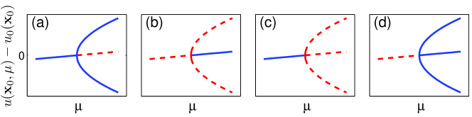
Figure 1: Schematic diagrams for the four types of pitchfork bifurcations in the GNLS equations (2.1). Plotted in this figure are deviations $u(\mathbf{x}_{0};\mu)-u_{0}(\mathbf{x}_{0})$ versus $\mu$ at a representative $\mathbf{x}_{0}$ position. Solid blue and dashed red lines indicate stable and unstable branches respectively.

Remark 3  In Theorem 4, the sign of $\alpha$ plays a critical role for the stability outcome. This sign can be determined as follows. From formula (3.8), we see that the sign of $\alpha$ is determined by the signs of $R$ and $\langle\psi,L_{00}^{-1}\psi\rangle$. We know from Theorem 1 that $R$ and $S$ have the same (opposite) sign if the bifurcated solitary waves appear on the right (left) side of $\mu=\mu_{0}$. We also know from formula (2.14) that $S$ and $P_{\pm}^{\prime}(\mu_{0})-P_{0}^{\prime}(\mu_{0})$ have the same sign. Using this information, the sign of $\alpha$ can be determined as follows.

1. If the bifurcated solitary waves appear on the right side of $\mu=\mu_{0}$, then the sign of $\alpha$ is equal to the sign of $\langle\psi,L_{00}^{-1}\psi\rangle$ multiplying the sign of $P_{\pm}^{\prime}(\mu_{0})-P_{0}^{\prime}(\mu_{0})$;

2. If the bifurcated solitary waves appear on the left side of $\mu=\mu_{0}$, then the sign of $\alpha$ is opposite of the sign of $\langle\psi,L_{00}^{-1}\psi\rangle$ multiplying the sign of $P_{\pm}^{\prime}(\mu_{0})-P_{0}^{\prime}(\mu_{0})$.

From this remark, we see that if the sign of $\langle\psi,L_{00}^{-1}\psi\rangle$ is known, then the sign of $\alpha$ can be read off from the structure of the power diagram (i.e., from which side of $\mu=\mu_{0}$ the bifurcated solutions reside and which of the power slopes $P_{\pm}^{\prime}(\mu_{0})$ and $P_{0}^{\prime}(\mu_{0})$ is larger). After the sign of $\alpha$ is obtained, stability of all the solution branches can then be read off again from the power diagram by Theorem 4. For instance, when $\langle\psi,L_{00}^{-1}\psi\rangle<0$ and the bifurcated solutions appear on the right side of the bifurcation point $\mu=\mu_{0}$, schematic power diagrams of all six possible bifurcation scenarios (with stability information indicated) are displayed in Fig. 2. This list of power diagrams is compiled according to the signs of $P_{0}^{\prime}(\mu_{0})$, $P_{\pm}^{\prime}(\mu_{0})$, and $P_{\pm}^{\prime}(\mu_{0})-P_{0}^{\prime}(\mu_{0})$. If $\langle\psi,L_{00}^{-1}\psi\rangle>0$, these power diagrams remain the same, but the stability of all branches is flipped (with “stable” changed to “unstable” and vise versa). If the bifurcated solutions appear on the left side of the bifurcation point $\mu=\mu_{0}$, their power diagrams (with stability information) can be similarly obtained.

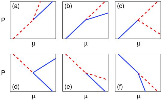
Figure 2: Six possible scenarios of the power diagram (with stability indicated) for pitchfork bifurcations in the GNLS equations (2.1) when $\langle\psi,L_{00}^{-1}\psi\rangle<0$ and the bifurcated solutions reside on the right side of the bifurcation point. Solid blue and dashed red lines indicate stable and unstable branches respectively.

One might notice that the power diagrams of pitchfork bifurcations in Fig. 2 split out to two rather than three branches at the bifurcation point, which is different from the solution-bifurcation diagrams in Fig. 1. The reason is that power slopes of the two bifurcated solution branches $u^{\pm}(\mathbf{x};\mu)$ are the same at the bifurcation point (see Theorem 2), thus one sees only two power branches instead of three [12].

The above results (i.e., Theorems 1–4) are valid for all real-valued solitary waves $u(\mathbf{x};\mu)$ in the GNLS equations (2.1), including both sign-definite (positive) and sign-indefinite (sign-changing) solitary waves. If the solitary waves are positive, then our stability results can be made stronger and more explicit. For positive solitary waves in Eq. (2.1), it is known that all eigenvalues in the linear-stability operator ${\cal L}$ are either purely real or purely imaginary (see Ref. [14], Theorem 5.2). In addition, linear stability of the solitary wave $u_{0}(\mathbf{x})$ at the bifurcation point can be determined by the generalized Vakhitov-Kolokolov stability criterion [14]. Furthermore, zero is the largest eigenvalue of $L_{0}$ and is simple [25], and $\langle\psi,L_{00}^{-1}\psi\rangle<0$ since operator $L_{00}$ is semi-negative definite. Using this information, together with Theorem 4 and Remark 3, we can obtain the following stronger and more explicit theorem for the linear stability of positive solitary waves near a pitchfork bifurcation point. This theorem derives linear stability of these solitary waves almost exclusively from their power diagram.

Theorem 5  Suppose solitary waves in the GNLS equations (2.1) are positive near a pitchfork bifurcation point $\mu=\mu_{0}$. If $P_{0}^{\prime}(\mu_{0})<0$, or zero is the $n$-th largest discrete eigenvalue of $L_{10}$ with $n\geq 3$, then these solitary waves (near the bifurcation point) are linearly unstable. If $P_{0}^{\prime}(\mu_{0})>0$, $P_{\pm}^{\prime}(\mu_{0})\neq 0$, and zero is the second largest and simple discrete eigenvalue of $L_{10}$, then

1. when the bifurcated solitary-wave branches $u^{\pm}(\mathbf{x};\mu)$ appear on the right side of $\mu=\mu_{0}$ and $P_{\pm}^{\prime}(\mu_{0})<P_{0}^{\prime}(\mu_{0})$, the smooth solution branch $u^{0}(\mathbf{x};\mu)$ is linearly stable for $\mu<\mu_{0}$ and unstable for $\mu>\mu_{0}$, whereas the bifurcated branches are linearly stable if $P_{\pm}^{\prime}(\mu_{0})>0$ and unstable if $P_{\pm}^{\prime}(\mu_{0})<0$;

2. when the bifurcated solitary waves appear on the right side of $\mu=\mu_{0}$ and $P_{\pm}^{\prime}(\mu_{0})>P_{0}^{\prime}(\mu_{0})$, the smooth solution branch is linearly unstable for $\mu<\mu_{0}$ and stable for $\mu>\mu_{0}$, whereas the bifurcated branches are always linearly unstable;

3. when the bifurcated solitary waves appear on the left side of $\mu=\mu_{0}$ and $P_{\pm}^{\prime}(\mu_{0})<P_{0}^{\prime}(\mu_{0})$, the smooth solution branch is linearly unstable for $\mu<\mu_{0}$ and stable for $\mu>\mu_{0}$, whereas the bifurcated branches are linearly stable if $P_{\pm}^{\prime}(\mu_{0})>0$ and unstable if $P_{\pm}^{\prime}(\mu_{0})<0$;

4. when the bifurcated solitary waves appear on the left side of $\mu=\mu_{0}$ and $P_{\pm}^{\prime}(\mu_{0})>P_{0}^{\prime}(\mu_{0})$, the smooth solution branch is linearly stable for $\mu<\mu_{0}$ and unstable for $\mu>\mu_{0}$, whereas the bifurcated branches are always linearly unstable.

In terms of solution-bifurcation diagrams, case (1) in this theorem belongs to pitchfork bifurcations of type (a) or (c) in Fig. 1, case (2) belongs to pitchfork bifurcations of type (b) in Fig. 1, case (3) belongs to pitchfork bifurcations of type (a) or (c) in Fig. 1 with the horizontal axis flipped, and case (4) belongs to pitchfork bifurcations of type (b) in Fig. 1 with the horizontal axis flipped. Thus for positive solitary waves in the GNLS equations (2.1), pitchfork bifurcations of type (d) in Fig. 1 (and its horizontal flip) cannot occur.

In terms of power-bifurcation diagrams, case (1) belongs to pitchfork bifurcations of type Fig. 2(b,c), case (2) belongs to pitchfork bifurcations of type Fig. 2(a), case (3) belongs to pitchfork bifurcations of type Fig. 2(d,e) with horizontal-axis flipping as well as branch-stability flipping, and case (4) belongs to pitchfork bifurcations of type Fig. 2(f) with horizontal-axis flipping as well as branch-stability flipping.

Remark 4  For positive solitary waves, pitchfork bifurcation cannot occur when the largest discrete eigenvalue of $L_{10}$ is zero. The reason is that for any linear Schrödinger operator, the eigenfunction of its largest eigenvalue is always positive (sign-definite) [25]. Thus for this largest zero eigenvalue of $L_{10}$, its eigenfunction $\psi$ is positive. Since $u_{0}(\mathbf{x})$ is also positive, then $\langle u_{0},\psi\rangle\neq 0$, which violates the conditions of pitchfork bifurcations in Theorem 1. Thus this case is not mentioned in Theorem 5.

4 Proofs of the main results

Proof of Theorem 3  The basic idea of the proof is that we first show the algebraic multiplicity of the zero eigenvalue in the linear-stability operator $\cal L$ is four at the bifurcation point $\mu=\mu_{0}$ and drops to two away from it, thus a pair of eigenvalues bifurcate out from the origin when $\mu\neq\mu_{0}$. This pair of eigenvalues must bifurcate along the real or imaginary axis since eigenvalues of $\cal L$ would appear as quadruples if this bifurcation were not along these two axes. Then we calculate this pair of eigenvalues near the bifurcation point $\mu=\mu_{0}$ by perturbation methods. We show that the perturbation series for these bifurcated eigenvalues can be constructed to all orders, with the leading-order terms given by Eqs. (3.7) and (3.9) for solitary waves on the smooth and bifurcated branches respectively.

At the pitchfork bifurcation point $\mu=\mu_{0}$ in Theorem 1, $(0,u_{0})^{T}$ and $(\psi,0)^{T}$ are eigenfunctions of the zero eigenvalue in ${\cal L}_{0}$ in view of Eq. (3.5). Here the superscript ‘$T$’ represents the transpose of a vector. Under the assumption in Theorem 3, ${\cal L}_{0}$ does not admit any additional eigenfunctions at the zero eigenvalue, thus the geometric multiplicity of this zero eigenvalue is two. Next we determine the algebraic multiplicity of this zero eigenvalue by examining its generalized eigenfunctions.

First, evaluating the relation (2.21) along the smooth solution branch $u^{0}(\mathbf{x};\mu)$ at $\mu=\mu_{0}$, we get

$$L_{10}\hskip 0.56917ptu^{0}_{\mu 0}=u_{0},$$ (4.1)

where $u^{0}_{\mu 0}$ is equal to $u^{0}_{\mu}$ evaluated at $\mu=\mu_{0}$. Thus,

$${\cal L}_{0}\left[\begin{array}[]{c}u^{0}_{\mu 0}\\ 0\end{array}\right]=\left[\begin{array}[]{c}0\\ u_{0}\end{array}\right],$$ (4.2)

which means that $(u^{0}_{\mu 0},0)^{T}$ is a generalized eigenfunction of the zero eigenvalue. The next-order generalized eigenfunction $(f_{2},g_{2})^{T}$ satisfies the equation

$${\cal L}_{0}\left[\begin{array}[]{c}f_{2}\\ g_{2}\end{array}\right]=\left[\begin{array}[]{c}u^{0}_{\mu 0}\\ 0\end{array}\right],$$ (4.3)

so the equation for $g_{2}$ is

$$L_{00}g_{2}=u^{0}_{\mu 0}.$$ (4.4)

Since $u_{0}$ is a homogeneous solution of this equation, $L_{00}$ is self-adjoint, and $\langle u_{0},u^{0}_{\mu 0}\rangle=P_{0}^{\prime}(\mu_{0})/2\neq 0$ by conditions (3.6), according to the Fredholm alternative theorem, Eq. (4.4) does not admit localized solutions for $g_{2}$, thus there are no additional generalized eigenfunctions for $(0,u_{0})^{T}$.

Next, we consider generalized eigenfunctions of ${\cal L}_{0}$ for $(\psi,0)^{T}$. The lowest-order generalized eigenfunction $(f_{1},g_{1})$ satisfies the equation

$${\cal L}_{0}\left[\begin{array}[]{c}f_{1}\\ g_{1}\end{array}\right]=\left[\begin{array}[]{c}\psi\\ 0\end{array}\right].$$ (4.5)

According to the assumption in Theorem 3, the kernel of $L_{00}$ contains a single localized function $u_{0}$, and $\langle u_{0},\psi\rangle=0$ in view of the conditions for pitchfork bifurcations in Theorem 1. Thus from the Fredholm alternative theorem, there exists a real localized function $L_{00}^{-1}\psi$. Consequently,

$${\cal L}_{0}\left[\begin{array}[]{c}0\\ L_{00}^{-1}\psi\end{array}\right]=\left[\begin{array}[]{c}\psi\\ 0\end{array}\right],$$ (4.6)

i.e., $(0,L_{00}^{-1}\psi)^{T}$ is a generalized eigenfunction of ${\cal L}_{0}$. The next-order generalized eigenfunction $(f_{2},g_{2})^{T}$ for $(\psi,0)^{T}$ satisfies the equation

$${\cal L}_{0}\left[\begin{array}[]{c}f_{2}\\ g_{2}\end{array}\right]=\left[\begin{array}[]{c}0\\ L_{00}^{-1}\psi\end{array}\right],$$ (4.7)

so the equation for $f_{2}$ is

$$L_{10}f_{2}=L_{00}^{-1}\psi.$$ (4.8)

Since $\psi$ is a homogeneous solution of this equation and $\langle\psi,L_{00}^{-1}\psi\rangle\neq 0$ by conditions (3.6), Eq. (4.8) does not admit any localized solutions by the Fredholm alternative theorem. Thus there are no additional generalized eigenfunctions for $(\psi,0)^{T}$.

The above analysis shows that ${\cal L}_{0}$ has two eigenfunctions and two generalized eigenfunctions at the zero eigenvalue, thus the algebraic multiplicity of the zero eigenvalue in ${\cal L}_{0}$ (at the bifurcation point) is four.

When $\mu\neq\mu_{0}$, on any solitary-wave branch $u^{0}(\mathbf{x};\mu)$ or $u^{\pm}(\mathbf{x};\mu)$, Eqs. (2.20)-(2.21) hold, thus $(0,u)^{T}$ is an eigenfunction of the zero eigenvalue in ${\cal L}$ (see Eq. (2.22)), and $(u_{\mu},0)^{T}$ is its generalized eigenfunction. This eigenfunction and generalized eigenfunction at $\mu\neq\mu_{0}$ are the counterparts of $(0,u_{0})^{T}$ and $(u^{0}_{\mu 0},0)^{T}$ at $\mu=\mu_{0}$ (see above), and they are induced by the phase invariance of Eq. (2.1). Under conditions in Theorem 3, we can further show, by similar analysis as above, that when $0<|\mu-\mu_{0}|\ll 1$, ${\cal L}$ does not admit any additional eigenfunctions or generalized eigenfunctions at the zero eigenvalue, thus the algebraic multiplicity of this zero eigenvalue in $\cal L$ is two.

Since the algebraic multiplicity of the zero eigenvalue in $\cal L$ is four at $\mu=\mu_{0}$ and drops to two when $\mu\neq\mu_{0}$, this means that when $\mu$ moves away from $\mu_{0}$, a pair of linear-stability eigenvalues must bifurcate out from the origin. Notice that the two multiplicities of the zero eigenvalue associated with the phase-invariance mode (2.22) persist when $\mu\neq\mu_{0}$ (see above), it is then clear that the two non-zero eigenvalues must bifurcate out from the bifurcation-induced zero eigenmode (3.2). Since eigenvalues of the linear-stability operator $\cal L$ always appear in quadruples (when they are complex) or in pairs (when they are real or purely imaginary) (see discussions below Eq. (2.19)), this bifurcated pair of eigenvalues then must be real or purely imaginary and be opposite of each other as a $\pm\lambda$ pair.

Next, we calculate this pair of bifurcated eigenvalues on the solution branches $u^{0}(\mathbf{x};\mu)$ and $u^{\pm}(\mathbf{x};\mu)$. Since at the bifurcation point the zero eigenvalue of ${\cal L}_{0}$ is not embedded inside ${\cal L}_{0}$’s continuous spectrum, this allows us to calculate this eigenvalue bifurcation by the perturbation methods (see Remark 1).

(a) Eigenvalue bifurcation along the smooth solution branch

We first calculate this eigenvalue bifurcation along the smooth solution branch $u^{0}(\mathbf{x};\mu)$. These solitary waves near the bifurcation point $\mu=\mu_{0}$ have the following perturbation series expansion

$$u^{0}(\mathbf{x};\mu)=\sum_{k=0}^{\infty}(\mu-\mu_{0})^{k}u_{k}(\mathbf{x}),$$ (4.9)

where $u_{1},u_{2},\dots$ are all real functions [12]. As a consequence, operators $L_{0}$ and $L_{1}$ on this smooth solution branch can be expanded as

$$L_{0}^{0}=\sum_{k=0}^{\infty}(\mu-\mu_{0})^{k}L_{0k},\quad L_{1}^{0}=\sum_{k=0}^{\infty}(\mu-\mu_{0})^{k}L_{1k}.$$ (4.10)

The linear-stability eigenmodes $(v,w,\lambda)$ bifurcated from the zero eigenmode (3.2) have the following perturbation series expansions:

$$v^{0}(\mathbf{x};\mu)=\sum_{k=0}^{\infty}(\mu-\mu_{0})^{k}v_{k}(\mathbf{x}),$$ (4.11)

$$w^{0}(\mathbf{x};\mu)=\lambda_{0}(\mu-\mu_{0})^{1/2}\sum_{k=0}^{\infty}(\mu-\mu_{0})^{k}w_{k}(\mathbf{x}),$$ (4.12)

$$\lambda^{0}(\mu)=i\lambda_{0}(\mu-\mu_{0})^{1/2}\left(1+\sum_{k=1}^{\infty}(\mu-\mu_{0})^{k}\lambda_{k}\right).$$ (4.13)

Below we construct these perturbation series solutions to all orders, and show that the leading-order expressions for the bifurcated eigenvalues $\lambda^{0}(\mu)$ are given by the formula (3.7).

We start by substituting the above perturbation expansions into the linear-stability eigenvalue problem (2.19). From these equations at various orders of $\mu-\mu_{0}$, we get a sequence of linear equations for $(v_{k},w_{k})$:

$$L_{10}v_{0}=0,$$ (4.14)

$$L_{00}w_{0}=v_{0},$$ (4.15)

$$L_{10}v_{1}=\lambda_{0}^{2}w_{0}-L_{11}v_{0},$$ (4.16)

$$L_{00}w_{1}=v_{1}+\lambda_{1}v_{0}-L_{01}w_{0},$$ (4.17)

$$L_{10}v_{2}=\lambda_{0}^{2}(w_{1}+\lambda_{1}w_{0})-(L_{11}v_{1}+L_{12}v_{0}),$$ (4.18)

$$L_{00}w_{2}=v_{2}+\lambda_{1}v_{1}+\lambda_{2}v_{0}-(L_{01}w_{1}+L_{02}w_{0}),$$ (4.19)

$$\dots\dots\dots$$

$$L_{10}v_{n+1}=\lambda_{0}^{2}\left(w_{n}+\sum_{k=1}^{n}\lambda_{k}w_{n-k}\right)-\sum_{k=1}^{n+1}L_{1k}v_{n+1-k},$$ (4.20)

$$L_{00}w_{n+1}=v_{n+1}+\sum_{k=1}^{n+1}\lambda_{k}v_{n+1-k}-\sum_{k=1}^{n+1}L_{0k}w_{n+1-k},$$ (4.21)

$$\dots\dots\dots$$

All these equations are inhomogeneous except the first equation for $v_{0}$. From the assumption in Theorem 3, the $v_{n}$ equations have a single homogeneous solution $\psi$, and the $w_{n}$ equations have a single homogeneous solution $u_{0}$. Since operators $L_{00}$ and $L_{10}$ in these equations are self-adjoint, the Fredholm alternative theorem says that the inhomogeneous equations above are solvable if and only if their right hand sides are orthogonal to their homogeneous solution. These orthogonality conditions, together with a scaling of the eigenfunction $(v,w)$, will determine the eigenvalue coefficients $\lambda_{n}$ as well as functions $(v_{n},w_{n})$ for all $n\geq 0$, as will be demonstrated below.

First we consider the $v_{0}$ equation (4.14). In view of the assumption in Theorem 3, the only solution to this equation (after eigenfunction scaling) is

$$v_{0}=\psi.$$ (4.22)

For the $w_{0}$ equation (4.15), due to the condition of $\langle u_{0},\psi\rangle=0$ for pitchfork bifurcations in Theorem 1, the Fredholm condition is satisfied, thus this equation admits a real localized solution $L_{00}^{-1}\psi$, and its general solution is

$$w_{0}=L_{00}^{-1}\psi+c_{0}u_{0},$$ (4.23)

where $c_{0}$ is a constant to be determined from the solvability condition of the $w_{1}$ equation later.

For the $v_{1}$ equation (4.16), it is solvable if and only if its right hand side is orthogonal to $\psi$. Utilizing the $v_{0}$ and $w_{0}$ solutions derived above, this orthogonality condition yields the formula for the eigenvalue coefficient $\lambda_{0}$ as

$$\lambda_{0}^{2}=\frac{\langle\psi,L_{11}\psi\rangle}{\langle\psi,L_{00}^{-1}\psi\rangle}.$$ (4.24)

According to our conditions (3.6), the denominator in the above formula is non-zero, thus $\lambda_{0}^{2}$ is well defined and is real. Later in this proof, we will derive a more explicit expression for $\lambda_{0}^{2}$ and show that it is non-zero as well [see Eq. (4.41)]. The above equation (4.24) gives two real or purely imaginary $\lambda_{0}$ values as a ‘$\pm$’ pair.

With the eigenvalue coefficient $\lambda_{0}$ given in (4.24), the orthogonality condition of the $v_{1}$ equation (4.16) is satisfied, thus the general solution for $v_{1}$ is

$$v_{1}=\widehat{v}_{1}+\lambda_{0}^{2}c_{0}L_{10}^{-1}u_{0}+d_{1}\psi,$$ (4.25)

where $\widehat{v}_{1}$ is a real and localized particular solution to the $v_{1}$ equation (4.16) but without the $c_{0}$ term in $w_{0}$ on its right hand side (see (4.23)). This $c_{0}$ term induces its own particular solution in $v_{1}$, which is the middle term in (4.25). In this term, $L_{10}^{-1}u_{0}$ is a real localized function which exists since $u_{0}$ is orthogonal to the function $\psi$ in the kernel of $L_{10}$. The last term in (4.25) is the homogeneous solution, where $d_{1}$ is a free real constant. Since this homogeneous term in $v_{1}$ can be lumped to the $v_{0}$ term as $v_{0}=[1+d_{1}(\mu-\mu_{0})]\psi$ and then eliminated by a scaling of the eigenfunction $(v,w)$, we will set $d_{1}=0$. A similar treatment will be applied to all higher $v_{n}$ solutions.

Now we consider the $w_{1}$ equation (4.17). Its solvability condition is that its right hand side be orthogonal to the homogeneous solution $u_{0}$. Noticing that $v_{0}$ is orthogonal to $u_{0}$ and $L_{01}$ is a real function, this solvability condition then reduces to

$$\langle u_{0},v_{1}\rangle-\langle L_{01}u_{0},w_{0}\rangle=0.$$ (4.26)

To simplify this condition, we recall the relation $L_{0}u^{0}(\mathbf{x};\mu)=0$. By inserting the expansions (4.9) and (4.10) for $L_{0}$ and $u^{0}(\mathbf{x};\mu)$ into this relation and collecting terms of $O(\mu-\mu_{0})$, we get

$$L_{01}u_{0}=-L_{00}u_{1}.$$ (4.27)

When this relation and the solutions of $w_{0}$ and $v_{1}$ are substituted into the solvability condition (4.26) and after simple algebra, this solvability condition then reduces to

$$c_{0}\lambda_{0}^{2}\langle u_{0},L_{10}^{-1}u_{0}\rangle=-\langle u_{0},\widehat{v}_{1}\rangle-\langle u_{1},\psi\rangle.$$ (4.28)

From Eq. (2.13) and conditions (3.6), $\langle u_{0},L_{10}^{-1}u_{0}\rangle\neq 0$. In addition, we will see from Eq. (4.41) later that $\lambda_{0}^{2}\neq 0$ as well. Thus the solvability condition (4.28) yields a unique real value for $c_{0}$ as

$$c_{0}=-\frac{\langle u_{0},\widehat{v}_{1}\rangle+\langle u_{1},\psi\rangle}{\lambda_{0}^{2}\langle u_{0},L_{10}^{-1}u_{0}\rangle}.$$ (4.29)

Consequently, the $w_{0}$ and $v_{1}$ solutions are now fully determined and are both real. In addition, with this $c_{0}$ value, the $w_{1}$ equation (4.17) is solvable, and its solution is

$$w_{1}=\widehat{w}_{1}+\lambda_{1}L_{00}^{-1}\psi+c_{1}u_{0},$$ (4.30)

where $\widehat{w}_{1}$ is a real and localized particular solution to the $w_{1}$ equation (4.17) but without the $\lambda_{1}$ term on its right hand side, and $c_{1}$ is a constant. The eigenvalue coefficient $\lambda_{1}$ and the constant $c_{1}$ will be determined from the solvability conditions of the $v_{2}$ and $w_{2}$ equations (4.18)-(4.19).

Next we use the method of induction to show that all higher-order terms in the perturbation series expansions (4.11)-(4.13) of $(v,w,\lambda)$ can be successively determined and are all real-valued. Suppose the $v_{0},v_{1},\dots,v_{n}$ and $w_{0},w_{1},\dots,w_{n-1}$ solutions have been fully obtained and are all real. In addition, suppose the $v_{n}$ solution is of the form

$$v_{n}=\widehat{v}_{n}+\lambda_{0}^{2}c_{n-1}L_{10}^{-1}u_{0},$$ (4.31)

where $\widehat{v}_{n}$ is a real and localized function, and $c_{n-1}$ is a real constant. Furthermore, suppose the $w_{n}$ solution is of the form

$$w_{n}=\widehat{w}_{n}+\lambda_{n}L_{00}^{-1}\psi+c_{n}u_{0},$$ (4.32)

where $\widehat{w}_{n}$ is a known real and localized function but the coefficients $\lambda_{n}$ and $c_{n}$ are not known yet. These assumptions are satisfied when $n=1$ (see above), and we now show if they hold for $n$ then they would still hold for $n+1$ as well. To determine $\lambda_{n}$, we use the solvability condition of the $v_{n+1}$ equation (4.20). Inserting (4.32) into this solvability condition, we readily find that

$$\lambda_{n}=\frac{\langle\psi,\sum_{k=1}^{n+1}L_{1k}v_{n+1-k}\rangle-\lambda_{0}^{2}\langle\psi,\widehat{w}_{n}+\sum_{k=1}^{n}\lambda_{k}w_{n-k}\rangle}{\lambda_{0}^{2}\langle\psi,L_{00}^{-1}\psi\rangle},$$ (4.33)

which is real. For this $\lambda_{n}$ value, the $v_{n+1}$ equation (4.20) is solvable, and its solution is of the form

$$v_{n+1}=\widehat{v}_{n+1}+\lambda_{0}^{2}c_{n}L_{10}^{-1}u_{0},$$ (4.34)

where $\widehat{v}_{n+1}$ is a real and localized particular solution to the $v_{n+1}$ equation but without the $c_{n}$ term in $w_{n}$ on its right hand side (see (4.32)). Notice that this $v_{n+1}$ solution is of the same form as $v_{n}$ in (4.31) but with the index $n$ changed to $n+1$.

To determine the constant $c_{n}$ in the above $w_{n}$ and $v_{n+1}$ solutions, we use the solvability condition of the $w_{n+1}$ equation (4.21), which is that its right hand side be orthogonal to the homogeneous solution $u_{0}$. Inserting the above $w_{n}$ and $v_{n+1}$ solutions into this solvability condition and utilizing the relation (4.27), we find that this solvability condition yields the $c_{n}$ value as

$$c_{n} = \frac{1}{\lambda_{0}^{2}\langle u_{0},L_{10}^{-1}u_{0}\rangle}\left[\langle u_{0},L_{01}\widehat{w}_{n}+\sum_{k=2}^{n+1}L_{0k}w_{n+1-k}\rangle\right.$$ (4.35)

$$\left.\hskip 14.22636pt-\langle u_{0},\widehat{v}_{n+1}+\sum_{k=1}^{n}\lambda_{k}v_{n+1-k}\rangle-\lambda_{n}\langle u_{1},\psi\rangle\right],$$

which is a real constant. With this $c_{n}$ value, the $w_{n}$ and $v_{n+1}$ solutions are now fully determined and are both real. In addition, the $w_{n+1}$ equation (4.21) is now solvable, and its general solution is

$$w_{n+1}=\widehat{w}_{n+1}+\lambda_{n+1}L_{00}^{-1}\psi+c_{n+1}u_{0},$$ (4.36)

where $\widehat{w}_{n+1}$ is a real and localized particular solution to the $w_{n+1}$ equation (4.21) but without the $\lambda_{n+1}$ term on its right hand side, and $c_{n+1}$ is a constant. This $w_{n+1}$ solution is of the same form as $w_{n}$ in (4.32) but with the index $n$ changed to $n+1$. This completes the induction process.

It is noted that in the above construction of the bifurcated eigenmodes, while $\lambda_{0}$ has two solutions $\lambda_{0\pm}$ (with $\lambda_{0+}=-\lambda_{0-}$) in view of Eq. (4.24), the higher coefficients $\lambda_{1},\lambda_{2},\dots$ as well as all $(v_{n},w_{n})$ functions in the expansions (4.11)-(4.13) depend on $\lambda_{0}^{2}$ only and are thus the same for both values of $\lambda_{0\pm}$. It is then clear that the above construction yields two eigenmodes $(v^{0}_{\pm},w^{0}_{\pm},\lambda^{0}_{\pm})$ which correspond to the two choices of the $\lambda_{0}$ values, and these two eigenmodes are related as

$$\lambda^{0}_{+}=-\lambda^{0}_{-},\quad v^{0}_{+}=v^{0}_{-},\quad w^{0}_{+}=-w^{0}_{-}.$$ (4.37)

In addition, $v^{0}_{\pm}$ is always real, and $w^{0}_{\pm}$, $\lambda^{0}_{\pm}$ are either real or purely imaginary. The asymptotic formula for the eigenvalues $\lambda^{0}_{\pm}$ is

$$(\lambda^{0})^{2}\to-\lambda_{0}^{2}\hskip 1.70709pt(\mu-\mu_{0}),\quad\mu\to\mu_{0},$$ (4.38)

where $\lambda_{0}^{2}$ is given in (4.24).

Finally, we simplify the $\lambda_{0}^{2}$ formula (4.24) and show that $-\lambda_{0}^{2}$ is equal to $\alpha$ as given in Eq. (3.8). To do so, we expand operator $L_{1}$ in (2.4) around $\mu=\mu_{0}$. Recalling the notations (2.9), we readily find $L_{11}$ in the expansion (4.10) of $L_{1}$ as

$$L_{11}=G_{2}u_{1}-1,$$ (4.39)

where $u_{1}$ is the $O(\mu-\mu_{0})$ term in $u^{0}(\mathbf{x};\mu)$’s expansion (4.9). The expression for $u_{1}$ has been obtained in Ref. [12] as

$$u_{1}=L_{10}^{-1}u_{0}+b_{1}\psi,$$ (4.40)

where $b_{1}$ is a real constant. Inserting the above two expressions into (4.24) and recalling the condition of $\langle G_{2},\psi^{3}\rangle=0$ for pitchfork bifurcations in Theorem 1 as well as the definition of constant $R$ in Eq. (2.11), we get a more explicit formula for $\lambda_{0}^{2}$ as

$$\lambda_{0}^{2}=-\frac{R}{\langle\psi,L_{00}^{-1}\psi\rangle}.$$ (4.41)

In view of the conditions for pitchfork bifurcations in Theorem 1, we see that $\lambda_{0}^{2}\neq 0$ as was mentioned before. Inserting this $\lambda_{0}^{2}$ formula into (4.38), the final asymptotic expression (3.7) for the bifurcated eigenvalues $\lambda^{0}(\mu)$ is then derived, with the constant $\alpha$ given by Eq. (3.8).

(b) Eigenvalue bifurcation along the bifurcated solution branches

Now we calculate eigenvalue bifurcations along the bifurcated solution branches $u^{\pm}(\mathbf{x};\mu)$. For convenience, we assume that these bifurcated solutions appear on the right side of $\mu=\mu_{0}$ (when $RS>0$, see Theorem 1). The other case of these bifurcated solutions appearing on the left side of $\mu=\mu_{0}$ can be similarly treated with trivial modifications, and both cases yield the same eigenvalue formula given in Eq. (3.9).

The bifurcated solitary waves near the bifurcation point $\mu=\mu_{0}$ have the following perturbation series expansion [12]

$$u^{\pm}(\mathbf{x};\mu)=\sum_{k=0}^{\infty}(\mu-\mu_{0})^{k/2}u_{k}(\mathbf{x}).$$ (4.42)

Since these solutions are assumed to exist on the right side of $\mu=\mu_{0}$, all functions $u_{1},u_{2},\dots$ in this expansion are real-valued. Operators $L_{0}$ and $L_{1}$ on these bifurcated solution branches are expanded as

$$L_{0}^{\pm}=\sum_{k=0}^{\infty}(\mu-\mu_{0})^{k/2}L_{0k},\quad L_{1}^{\pm}=\sum_{k=0}^{\infty}(\mu-\mu_{0})^{k/2}L_{1k},$$ (4.43)

and all terms in these expansions are real-valued too. Note that quantities $u_{k},L_{0k},L_{1k},k=1,2,\dots$ in these expansions are different from those in previous expansions (4.9)-(4.10). The linear-stability eigenmodes $(v,w,\lambda)$ bifurcated from the zero eigenmode (3.2) now have the perturbation series expansions

$$v^{\pm}(\mathbf{x};\mu)=\sum_{k=0}^{\infty}(\mu-\mu_{0})^{k/2}v_{k}(\mathbf{x}),$$ (4.44)

$$w^{\pm}(\mathbf{x};\mu)=\lambda_{0}\sum_{k=0}^{\infty}(\mu-\mu_{0})^{k/2}w_{k}(\mathbf{x}),$$ (4.45)

$$\lambda^{\pm}(\mu)=i\lambda_{0}(\mu-\mu_{0})^{1/2}\left(1+\sum_{k=1}^{\infty}(\mu-\mu_{0})^{k/2}\lambda_{k}\right).$$ (4.46)

Below we construct these perturbation series solutions to all orders.

Before this construction, we first derive a few relations on functions $u_{0},u_{1},u_{2}$ and $u_{3}$ in (4.42), which will be needed in later calculations. By inserting expansions (4.42) and (4.43) into equations (2.20) and (2.21) and at suitable orders, we get the following relations

$$L_{01}u_{0}=-L_{00}u_{1},$$ (4.47)

$$L_{02}u_{0}=-L_{01}u_{1}-L_{00}u_{2},$$ (4.48)

$$L_{11}u_{1}=2(u_{0}-L_{10}u_{2}),$$ (4.49)

$$L_{12}u_{1}=2u_{1}-2L_{11}u_{2}-3L_{10}u_{3}.$$ (4.50)

In addition,

$$u_{1}=b_{1}\psi,$$ (4.51)

where $b_{1}=\pm\sqrt{6R/S}$ which is non-zero [12]. Notice that $b_{1}$ is also real-valued here since $RS>0$ by our earlier assumption.

We now substitute the perturbation expansions (4.44)-(4.46) into the linear-stability eigenvalue problem (2.19). From various orders of $(\mu-\mu_{0})^{1/2}$, we get a sequence of linear equations for $(v_{k},w_{k})$ as

$$L_{10}v_{0}=0,$$ (4.52)

$$L_{00}w_{0}=0,$$ (4.53)

$$L_{10}v_{1}=\lambda_{0}^{2}w_{0}-L_{11}v_{0},$$ (4.54)

$$L_{00}w_{1}=v_{0}-L_{01}w_{0},$$ (4.55)

$$L_{10}v_{2}=\lambda_{0}^{2}(w_{1}+\lambda_{1}w_{0})-(L_{11}v_{1}+L_{12}v_{0}),$$ (4.56)

$$L_{00}w_{2}=v_{1}+\lambda_{1}v_{0}-(L_{01}w_{1}+L_{02}w_{0}),$$ (4.57)

$$\dots\dots\dots$$

$$L_{10}v_{n+1}=\lambda_{0}^{2}\left(w_{n}+\sum_{k=1}^{n}\lambda_{k}w_{n-k}\right)-\sum_{k=1}^{n+1}L_{1k}v_{n+1-k},$$ (4.58)

$$L_{00}w_{n+1}=v_{n}+\sum_{k=1}^{n}\lambda_{k}v_{n-k}-\sum_{k=1}^{n+1}L_{0k}w_{n+1-k},$$ (4.59)

$$\dots\dots\dots$$

In view of the assumption in Theorem 3, the solution to the $v_{0}$ equation (4.52), after eigenfunction rescaling, can be taken as

$$v_{0}=u_{1},$$ (4.60)

where $u_{1}$ is given in (4.51). The solution to the $w_{0}$ equation (4.53) is

$$w_{0}=c_{0}u_{0},$$ (4.61)

where $c_{0}$ is a constant to be determined. When these $(v_{0},w_{0})$ solutions are inserted into the $(v_{1},w_{1})$ equations (4.54)-(4.55) and relations (4.47), (4.49) utilized, we find that the solvability conditions of the $(v_{1},w_{1})$ equations are automatically satisfied due to the condition of $\langle u_{0},\psi\rangle=0$ for pitchfork bifurcations in Theorem 1, and these $(v_{1},w_{1})$ equations admit localized solutions of the form

$$v_{1}=2(u_{2}-L_{10}^{-1}u_{0})+c_{0}\lambda_{0}^{2}L_{10}^{-1}u_{0},$$ (4.62)

and

$$w_{1}=L_{00}^{-1}u_{1}+c_{0}u_{1}+c_{1}u_{0},$$ (4.63)

where $L_{10}^{-1}u_{0}$ and $L_{00}^{-1}u_{1}$ are localized functions and $c_{1}$ is another constant. It is noted that the homogeneous solution (in proportion to $u_{1}$) to the $v_{1}$ equation is not included in the above $v_{1}$ solution since this term can be lumped into the $v_{0}$ term and then eliminated by a rescaling of the eigenfunction $(v,w)$ — the same treatment we have applied previously in case (a) (see Eq. (4.25)).

Now we consider the $(v_{2},w_{2})$ equations (4.56)-(4.57). Inserting the above $(v_{0},v_{1},w_{0},w_{1})$ solutions into the right hand side of the $v_{2}$ equation, utilizing the relations (4.47)-(4.50) and after simple algebra, the solvability condition of this $v_{2}$ equation, which requires that its right hand side be orthogonal to the homogeneous solution $u_{1}$, yields

$$\lambda_{0}^{2}=(2-c_{0}\lambda_{0}^{2})\frac{\langle u_{1},u_{1}\rangle+2\langle u_{0},u_{2}\rangle-2\langle u_{0},L_{10}^{-1}u_{0}\rangle}{\langle u_{1},L_{00}^{-1}u_{1}\rangle}.$$ (4.64)

It is noted that $u_{1}$ is proportional to $\psi$ and is nonzero, see Eq. (4.51). Thus due to the conditions (3.6), the denominator in the above equation is nonzero, i.e., $\langle u_{1},L_{00}^{-1}u_{1}\rangle\neq 0$. From the expansion (4.42) of the solutions $u^{\pm}(\mathbf{x};\mu)$ and the condition $\langle u_{0},\psi\rangle=0$, we see that the expansion for the power function $P_{\pm}(\mu)$ is

$$P_{\pm}(\mu)=\langle u_{0},u_{0}\rangle+P_{\pm}^{\prime}(\mu_{0})(\mu-\mu_{0})+O[(\mu-\mu_{0})^{3/2}],$$ (4.65)

where

$$P_{\pm}^{\prime}(\mu_{0})=\langle u_{1},u_{1}\rangle+2\langle u_{0},u_{2}\rangle$$ (4.66)

is the power slope at the bifurcation point $\mu=\mu_{0}$. From Eq. (2.14) in Theorem 2, we also know that

$$P_{+}^{\prime}(\mu_{0})=P_{-}^{\prime}(\mu_{0})=2\langle u_{0},L_{10}^{-1}u_{0}\rangle+\frac{6R^{2}}{S}.$$ (4.67)

Using these relations as well as Eq. (4.51), the solvability condition (4.64) of the $v_{2}$ equation reduces to

$$\lambda_{0}^{2}=(2-c_{0}\lambda_{0}^{2})\,\frac{R}{\langle\psi,L_{00}^{-1}\psi\rangle}.$$ (4.68)

From the conditions for pitchfork bifurcations in Theorem 1, $R\neq 0$, thus $\lambda_{0}^{2}\neq 0$.

Carrying similar calculations to the $w_{2}$ equation (4.57) and recalling the formula (2.13), the solvability condition of this $w_{2}$ equation yields

$$2-c_{0}\lambda_{0}^{2}=\frac{2P_{\pm}^{\prime}(\mu_{0})}{P_{0}^{\prime}(\mu_{0})}.$$ (4.69)

When this equation is inserted into (4.68), an expression for $\lambda_{0}^{2}$ is then obtained as

$$\lambda_{0}^{2}=\frac{2P_{\pm}^{\prime}(\mu_{0})}{P_{0}^{\prime}(\mu_{0})}\,\frac{R}{\langle\psi,L_{00}^{-1}\psi\rangle},$$ (4.70)

which is real and nonzero. Inserting this $\lambda_{0}^{2}$ formula into (4.69), the constant $c_{0}$ can be obtained and is also real.

When $\lambda_{0}$ and $c_{0}$ are given by Eqs. (4.69)-(4.70), the solvability conditions of the $(v_{2},w_{2})$ equations (4.56)-(4.57) are satisfied. Utilizing the relation (4.47), the $(v_{2},w_{2})$ solutions are of the form

$$v_{2}=\widehat{v}_{2}+\lambda_{0}^{2}(c_{1}+\lambda_{1}c_{0})L_{10}^{-1}u_{0},$$ (4.71)

and

$$w_{2}=\widehat{w}_{2}+\lambda_{1}L_{00}^{-1}u_{1}+c_{1}u_{1}+c_{2}u_{0},$$ (4.72)

where $\widehat{v}_{2}$ and $\widehat{w}_{2}$ are localized functions which satisfy equations (4.56)-(4.57) but without the $c_{1}$ and $\lambda_{1}$ terms on their right hand sides, and $c_{2}$ is another constant. These constants $\lambda_{1},c_{1}$ and $c_{2}$ will be determined from the solvability conditions of the higher $(v_{n},w_{n})$ equations.

Using the method of induction and after straightforward algebra, we can show that the perturbation series solution (4.44)-(4.46) for the eigenmode $(v,w,\lambda)$ can be determined to all orders. In addition, the $(v_{n},w_{n})$ terms for $n\geq 2$ are of the form

$$v_{n}=\widehat{v}_{n}+\lambda_{0}^{2}(c_{n-1}+\lambda_{n-1}c_{0})L_{10}^{-1}u_{0},\quad n\geq 2,$$ (4.73)

and

$$w_{n}=\widehat{w}_{n}+\lambda_{n-1}L_{00}^{-1}u_{1}+c_{n-1}u_{1}+c_{n}u_{0},\quad n\geq 2,$$ (4.74)

where $\widehat{v}_{n}$ and $\widehat{w}_{n}$ are certain localized functions, and $\lambda_{n-1},c_{n-1},c_{n}$ are constants. Since this induction calculation is analogous to that for case (a) in the earlier text, the details are omitted here.

In the above construction of the bifurcated eigenmodes, since $\lambda_{0}$ has two solutions from Eq. (4.70), two eigenmodes are then obtained. The eigenvalues of these two modes are either real or purely imaginary and are opposite of each other. From the perturbation expansion of these eigenvalues in Eq. (4.46) as well as Eq. (4.70), we see that the asymptotic formula for these eigenvalues near the bifurcation point is

$$(\lambda^{\pm})^{2}\to-\frac{2P_{\pm}^{\prime}(\mu_{0})}{P_{0}^{\prime}(\mu_{0})}\,\frac{R}{\langle\psi,L_{00}^{-1}\psi\rangle}\,(\mu-\mu_{0}),\quad\mu\to\mu_{0},$$ (4.75)

which is the same as the formula (3.9) in Theorem 3. This completes the proof of Theorem 3. $\Box$

Proof of Theorem 4  From the assumptions in Theorem 4, the solitary wave $u_{0}(\mathbf{x})$ at the bifurcation point $\mu=\mu_{0}$ is linearly stable; and when $0<|\mu-\mu_{0}|\ll 1$, the only instability-inducing eigenvalue bifurcation is from the origin. In Theorem 3, we have shown that from the origin, a single pair of eigenvalues $\pm\lambda$ in ${\cal L}$ bifurcate out along the real or imaginary axis. Thus the linear stability of these solitary waves near $\mu=\mu_{0}$ is determined entirely by whether this pair of eigenvalues are real or purely imaginary. On the smooth solitary wave branch $u^{0}(\mathbf{x};\mu)$, this pair of eigenvalues are given asymptotically by Eq. (3.7). Thus if $\alpha>0$, these eigenvalues are real when $\mu>\mu_{0}$ and imaginary when $\mu<\mu_{0}$, hence the solitary waves are linearly unstable when $\mu>\mu_{0}$ and linearly stable when $\mu<\mu_{0}$. If $\alpha<0$, the situation is just the opposite. In both cases, stability switches at the bifurcation point. On the bifurcated solitary branches $u^{\pm}(\mathbf{x};\mu)$, the bifurcated eigenvalues are given asymptotically by Eq. (3.9). The formula (3.10) for the constant $\beta$ shows that when the two power slopes $P_{0}^{\prime}(\mu_{0})$ and $P_{\pm}^{\prime}(\mu_{0})$ have the same sign, $\beta$ and $\alpha$ would have the opposite sign, meaning that eigenvalues for the $u^{\pm}(\mathbf{x};\mu)$ and $u^{0}(\mathbf{x};\mu)$ branches bifurcate along perpendicular directions from the origin, hence these solution branches have opposite linear stability. On the other hand, if the two power slopes $P_{0}^{\prime}(\mu_{0})$ and $P_{\pm}^{\prime}(\mu_{0})$ have the opposite sign, $\beta$ and $\alpha$ would have the same sign, hence the $u^{\pm}(\mathbf{x};\mu)$ and $u^{0}(\mathbf{x};\mu)$ branches would have the same linear stability. This completes the proof of Theorem 4. $\Box$

Proof of Theorem 5  If zero is the $n$-th largest discrete eigenvalue of $L_{10}$ with $n\geq 3$, then $L_{10}$ has two positive eigenvalues, hence the positive solitary wave $u_{0}(\mathbf{x})$ at the bifurcation point $\mu=\mu_{0}$ is linearly unstable by the generalized Vakhitov-Kolokolov stability criterion [14]. If zero is the second-largest discrete eigenvalue of $L_{10}$, then $L_{10}$ has one positive eigenvalue. Meanwhile, by the conditions of pitchfork bifurcations in Theorem 1, $\langle u_{0},\psi\rangle=0$. In this case, if $P_{0}^{\prime}(\mu_{0})<0\ (>0)$, then the positive solitary wave $u_{0}(\mathbf{x})$ is linearly unstable (stable) by the generalized Vakhitov-Kolokolov stability criterion [14]. When $u_{0}(\mathbf{x})$ is linearly unstable, solitary waves near the bifurcation point $\mu=\mu_{0}$ are clearly also linearly unstable.

Next we consider the case when $P_{0}^{\prime}(\mu_{0})>0$, $P_{\pm}^{\prime}(\mu_{0})\neq 0$ and zero is the second largest and simple discrete eigenvalue of $L_{10}$. In this case, $u_{0}(\mathbf{x})$ at the bifurcation point is linearly stable (see above). In addition, for positive solitary waves, all eigenvalues in ${\cal L}$ are real or purely imaginary (see Ref. [14], Theorem 5.2), thus no complex eigenvalues can bifurcate out when $\mu\neq\mu_{0}$. So the assumptions in Theorem 4 are satisfied. Since $u_{0}(\mathbf{x})$ is positive, zero is then the largest eigenvalue of $L_{00}$ and is simple [25], and $\langle\psi,L_{00}^{-1}\psi\rangle<0$ as $L_{00}$ is semi-negative definite and $\psi\neq 0$. In addition, zero is a simple eigenvalue of $L_{10}$, $P_{0}^{\prime}(\mu_{0})\neq 0$ and $P_{\pm}^{\prime}(\mu_{0})\neq 0$ by our assumptions above. Thus the conditions of Theorem 4 are also met. Hence Theorem 4 can be applied. Using this theorem, together with Remark 3 and the fact of $\langle\psi,L_{00}^{-1}\psi\rangle<0$, we can then prove the results in the four cases of Theorem 5 as below.

1. When the bifurcated solitary waves $u^{\pm}(\mathbf{x};\mu)$ appear on the right side of $\mu=\mu_{0}$ and $P_{\pm}^{\prime}(\mu_{0})<P_{0}^{\prime}(\mu_{0})$, $\alpha$ is positive by Remark 3. Then by Theorem 4, the smooth solution branch $u^{0}(\mathbf{x};\mu)$ is stable for $\mu<\mu_{0}$ and unstable for $\mu>\mu_{0}$. Regarding the bifurcated branches, they and the unstable smooth branch (on the right side of $\mu=\mu_{0}$) should have the opposite (same) stability when $P_{0}^{\prime}(\mu_{0})$ and $P_{\pm}^{\prime}(\mu_{0})$ have the same (opposite) sign. Since $P_{0}^{\prime}(\mu_{0})>0$, these bifurcated branches are then stable when $P_{\pm}^{\prime}(\mu_{0})>0$ and unstable when $P_{\pm}^{\prime}(\mu_{0})<0$.

2. When the bifurcated solitary waves appear on the right side of $\mu=\mu_{0}$ and $P_{\pm}^{\prime}(\mu_{0})>P_{0}^{\prime}(\mu_{0})>0$, $\alpha$ is negative by Remark 3. Thus the smooth solution branch is unstable for $\mu<\mu_{0}$ and stable for $\mu>\mu_{0}$. Since $P_{\pm}^{\prime}(\mu_{0})$ and $P_{0}^{\prime}(\mu_{0})$ are now both positive, the bifurcated branches then have the opposite stability of the stable smooth branch (on the right side of $\mu=\mu_{0}$) are thus always unstable.

3. When the bifurcated solitary waves appear on the left side of $\mu=\mu_{0}$ and $P_{\pm}^{\prime}(\mu_{0})<P_{0}^{\prime}(\mu_{0})$, $\alpha$ is negative by Remark 3. Then by Theorem 4, the smooth solution branch is unstable for $\mu<\mu_{0}$ and stable for $\mu>\mu_{0}$. The bifurcated branches (with $\mu<\mu_{0}$) are stable (opposite of the unstable smooth branch) if $P_{\pm}^{\prime}(\mu_{0})>0$ and unstable (same as the unstable smooth branch) if $P_{\pm}^{\prime}(\mu_{0})<0$.

4. When the bifurcated solitary waves appear on the left side of $\mu=\mu_{0}$ and $P_{\pm}^{\prime}(\mu_{0})>P_{0}^{\prime}(\mu_{0})>0$, $\alpha$ is positive by Remark 3; hence by Theorem 4, the smooth solution branch is stable for $\mu<\mu_{0}$ and unstable for $\mu>\mu_{0}$. Since both $P_{\pm}^{\prime}(\mu_{0})$ and $P_{0}^{\prime}(\mu_{0})$ are now positive, the bifurcated branches are always unstable (opposite of the stable smooth branch on the left side of $\mu=\mu_{0}$). This completes the proof of Theorem 5. $\Box$

5 Numerical examples

In this section, we use a few numerical examples to illustrate and confirm the above analytical stability results. These examples contain both positive and sign-indefinite solitary waves under various self-focusing and self-defocusing nonlinearities in one and higher spatial dimensions.

Example 1  Our first example is the one-dimensional GNLS equation (2.1) with a symmetric double-well potential and cubic-quintic nonlinearity,

$$iU_{t}+U_{xx}-V(x)U+|U|^{2}U-0.25|U|^{4}U=0,$$ (5.1)

where the symmetric double-well potential $V(x)$ is taken as

$$V(x)=-2.8\left[\mbox{sech}^{2}(x+1.5)+\mbox{sech}^{2}(x-1.5)\right]$$ (5.2)

and is shown in Fig. 3(a). Pitchfork bifurcations of positive solitary waves in this equation have been reported in [12], and the power diagram for these bifurcations is displayed in Fig. 3(b). This power diagram shows that two pitchfork bifurcations occur at points ‘A,B’ of the power diagram. At positions ‘c,d,e’, profiles of solitary waves are shown in Fig. 3(c,d,e) respectively. It is seen that solitary waves at positions ‘c,d’ are symmetric, while solitary waves at position ‘e’ are asymmetric. Thus symmetry-breaking bifurcations occur at both ‘A,B’ points. In particular, the c-d power branch is the symmetric (smooth) branch, and the e-branch is the asymmetric (bifurcated) branch.

Since solitary waves in this example are positive, Theorem 5 applies. It is known that for both pitchfork bifurcations at points ‘A,B’, zero is the second largest eigenvalue of $L_{10}$ [12]. In addition, the power diagram in Fig. 3(b) shows that at both ‘A,B’ points, $0<P_{\pm}^{\prime}(\mu_{0})<P_{0}^{\prime}(\mu_{0})$. Thus Theorem 5 predicts that near the bifurcation point ‘A’, the smooth (symmetric) branch is linearly stable on the left side of ‘A’ and unstable on the right side of ‘A’, and the bifurcated (asymmetric) branch (which is on the right side of ‘A’) is linearly stable. Regarding the bifurcation point ‘B’, Theorem 5 predicts that the symmetric branch is unstable on the left side of ‘B’ and stable on the right side of ‘B’, and the bifurcated asymmetric branch (which is on the left side of ‘B’) is linearly stable.

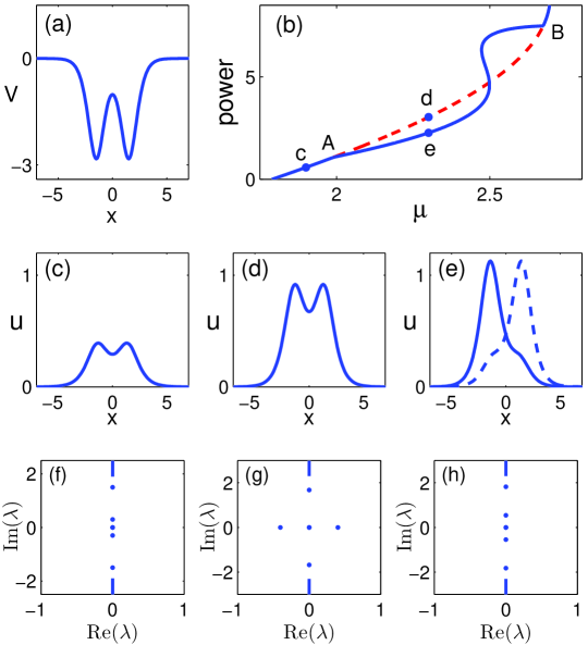
Figure 3: Pitchfork bifurcations of solitary waves and their linear-stability behaviors in Example 1. (a) The potential (5.2); (b) the power diagram (solid blue and dashed red indicate stable and unstable solutions respectively); (c,d,e) profiles of solitary waves at positions of the same letters in (b); the two asymmetric solitary waves in (e) are mirror images of each other with respect to $x$; (f,g,h) linear-stability spectra of the solitary waves in (c,d,e) respectively.

Numerically we have found that these analytical predictions are entirely correct. Specifically, we have found numerically that the segment of the symmetric branch between points ‘A,B’ is linearly unstable, and the other segments/branches of the power diagram are all linearly stable. This stability information is indicated by the solid blue and dashed red lines in Fig. 3(b) for stable and unstable parts respectively. To support this stability result, the linear-stability spectra for solitary waves at locations ‘c,d,e’ of the power diagram are numerically computed by the Fourier collocation method [14], and the results are displayed in Fig. 3(f,g,h). It is seen that the spectrum at ‘d’ contains a positive eigenvalue, hence its symmetric solitary wave is linearly unstable. The spectra at ‘c,e’, on the other hand, lie entirely on the imaginary axis, thus those solitary waves are linearly stable. These numerical stability results agree completely with the above analytical predictions.

The reader may notice that the asymmetric ‘e’-branch in Fig. 3(b) contains two additional saddle-node (fold) bifurcations. As was explained in [20, 21], there is no stability switching at saddle-node bifurcations in the GNLS equations (2.1), thus it is not surprising that the entire asymmetric ‘e’-branch in Fig. 3(b) is linearly stable despite these saddle-node bifurcations.

Example 2  Our second example is the one-dimensional GNLS equation (2.1) with self-focusing cubic nonlinearity and a periodic potential,

$$iU_{t}+U_{xx}-V(x)U+|U|^{2}U=0,$$ (5.3)

where the potential $V(x)$ is

$$V(x)=6\sin^{2}x.$$ (5.4)

This equation admits a family of sign-indefinite solitary waves of the form (2.2) in the semi-infinite bandgap [11], and its power diagram is shown in Fig. 4(a). This power diagram contains three branches which are connected with each other. At the intersection point ‘A’ between the lower and middle branches, a pitchfork bifurcation occurs. This pitchfork bifurcation is better seen in Fig. 4(b), which shows an amplification of the power diagram in Fig. 4(a) around this intersection point. Solitary waves on the lower power branch are anti-symmetric (see Fig. 4(c)), whereas solitary waves on the middle power branch are asymmetric (see Fig. 4(d)), hence a symmetry-breaking bifurcation occurs at point ‘A’.

At this bifurcation point ‘A’, we have checked numerically that $\langle\psi,L_{00}^{-1}\psi\rangle<0$. In addition, the power diagram in Fig. 4(b) shows that the bifurcated (asymmetric) solitary waves appear on the right side ‘A’, and $P_{\pm}^{\prime}(\mu_{0})>P_{0}^{\prime}(\mu_{0})>0$. Thus, Remark 3 gives $\alpha<0$. We have also checked that the solitary wave at point ‘A’ is linearly stable, and near this point no complex eigenvalues appear. Then Theorem 4 predicts that the lower branch is unstable on the left side of ‘A’ and stable on the right side of ‘A’. In addition, the bifurcated asymmetric branch is unstable.

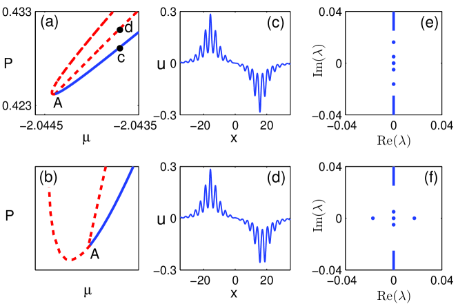
Figure 4: Pitchfork bifurcations of solitary waves and their linear-stability behaviors in Example 2. (a) The power diagram (solid blue for stable branches and dashed red for unstable ones); (b) amplification of the power diagram in (a) near the pitchfork bifurcation point ‘A’; (c,d) profiles of solitary waves at locations ‘c,d’ of the power diagram in (a); (e,f) linear-stability spectra for solitary waves in (c,d) respectively.

Numerically we have found that these analytical predictions are again all correct. Specifically, we have determined the stability of these solitary waves through computation of their linear-stability spectra, and the stability results are indicated on the power diagram in Fig. 4(a,b), where the stable and unstable branches are marked as solid blue and dashed red lines respectively. We see that these stability results are in full agreement with the above analytical predictions. To corroborate these stability results, the full linear-stability spectra for solitary waves at locations ‘c,d’ of Fig. 4(a) are displayed in Fig. 4(e,f). These spectra confirm that the anti-symmetric solitary wave [Fig. 4(c)] at location ‘c’ of the lower power branch is indeed linearly stable, whereas the asymmetric solitary wave [Fig. 4(d)] at location ‘d’ of the middle branch is indeed linearly unstable. The unstable eigenvalue at location ‘d’ is real positive, and it bifurcates out from the pitchfork bifurcation point ‘A’, in agreement with our theory.

Example 3  Our third example is the seventh-power GNLS equation with a symmetric double-well potential,

$$iU_{t}+U_{xx}-V(x)U+|U|^{6}U=0,$$ (5.5)

where the potential $V(x)$ is

$$V(x)=-3\>\mbox{sech}^{2}(x+1)-3\>\mbox{sech}^{2}(x-1),$$ (5.6)

which is shown in Fig. 5(b). This equation admits a family of positive solitary waves whose power diagram is displayed in Fig. 5(a). This power diagram shows that a pitchfork bifurcation occurs at the point ‘A’. On the upper b-$c_{1}$ branch, solitary waves are symmetric (see Fig. 5(b,c)), whereas on the lower $c_{2}$ branch, solitary waves are asymmetric (see Fig. 5(c)).

At the pitchfork bifurcation point ‘A’, we have checked that zero is the second largest eigenvalue of $L_{10}$. Thus from the power diagram in Fig. 5(a), Theorem 5 predicts that the symmetric b-$c_{1}$ branch is stable on the left side of ‘A’ and unstable on the right side of ‘A’. In addition, the asymmetric $c_{2}$ branch is unstable. These analytical predictions fully agree with the numerical stability results in Fig. 5(a) (where the stable and unstable solutions are indicated). These stability results are further corroborated in Fig. 5(d,e,f), where linear-stability spectra for solitary waves at locations ’b, $c_{1}$, $c_{2}$’ are displayed.

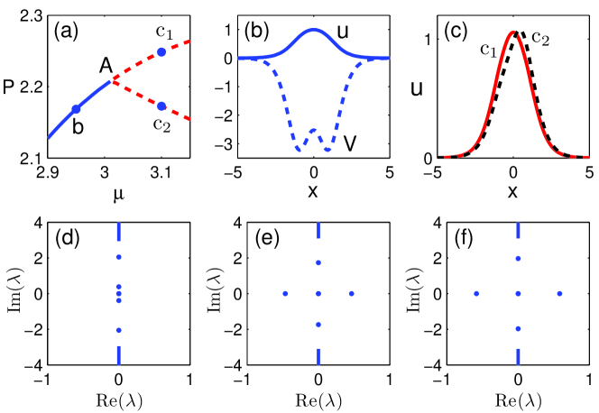
Figure 5: Pitchfork bifurcations of solitary waves and their linear-stability behaviors in Example 3. (a) The power diagram (solid blue is stable and dashed red unstable); (b) profiles of the potential $V(x)$ (dashed) and the solitary wave (solid) at location ‘b’ of the power diagram; (c) solitary wave profiles at locations ‘$c_{1}$’ (solid) and ‘$c_{2}$’ (dashed) of the power diagram; (e,f,g) linear-stability spectra for solitary waves at locations ‘b, $c_{1}$, $c_{2}$’ respectively.

In this example, after the pitchfork bifurcation occurs (i.e., on the right side of ‘A’), both the symmetric and asymmetric solution branches are linearly unstable. A similar bifurcation was reported numerically in [9] for the eleventh-power nonlinearity but was not found for the present seventh-power nonlinearity.

Example 4   Our last example is the two-dimensional GNLS equation with self-defocusing cubic nonlinearity and a symmetric double-well potential,

$$iU_{t}+U_{xx}+U_{yy}-V(x,y)U-|U|^{2}U=0,$$ (5.7)

where the potential $V(x,y)$ is

$$V(x,y)=-6\left(e^{-[(x+1.5)^{2}+y^{2}]}+e^{-[(x-1.5)^{2}+y^{2}]}\right),$$ (5.8)

which is shown in Fig. 6(a). This equation admits a family of sign-indefinite solitary waves (2.2) whose power diagram is given in Fig. 6(b). It is seen that a pitchfork bifurcation occurs at the point ‘A’. At positions ’d,e,f’ of the power diagram, profiles of the solitary waves are displayed in Fig. 6(d,e,f). Solitary waves at ‘d,e’ are anti-symmetric in $x$ and symmetric in $y$, whereas the solitary wave at ‘f’ is asymmetric in $x$ and symmetric in $y$. Thus this pitchfork bifurcation is also a symmetry-breaking bifurcation.

At this bifurcation point, we have checked numerically that zero is the largest eigenvalue of $L_{10}$, and $\langle\psi,L_{00}^{-1}\psi\rangle>0$. In addition, the solitary wave at point ‘A’ is linearly stable, and the solitary waves nearby do not possess complex eigenvalues. Thus from Remark 3 and the power diagram in Fig. 6(b), Theorem 4 predicts that the anti-symmetric solution branch is unstable on the left side of ‘A’ and stable on the right side of ‘A’, and the bifurcated asymmetric branch is stable. These predictions agree with our numerical stability results shown in Fig. 6(b). The numerical-stability results are further illustrated in Fig. 6(g,h,i), where the stability spectra for solitary waves in Fig. 6(d,e,f) are plotted. These spectra corroborate the numerical-stability results in the power diagram of Fig. 6(b) and support our analytical predictions.

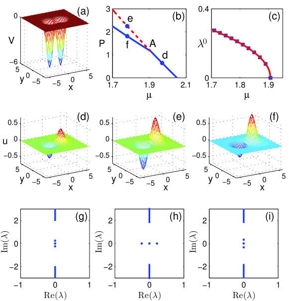
Figure 6: Pitchfork bifurcations of solitary waves and their linear-stability behaviors in Example 4. (a) The two-dimensional double-well potential (5.8); (b) the power diagram (solid blue is stable and dashed red unstable); (c) the unstable eigenvalue $\lambda^{0}$ versus $\mu$ on the anti-symmetric solution branch of (b) [squares: numerical values; solid red line: analytical prediction from formula (3.7)]; (d,e,f) profiles of solitary waves at locations ‘d,e,f’ of the power diagram in (b); (g,h,i) stability spectra for solitary waves in (d,e,f) respectively.

In the previous examples, our comparison between analytical and numerical stability results was qualitative. Here for this example 4, we will also make a quantitative comparison on unstable eigenvalues in order to completely verify our eigenvalue formulae in Theorem 3. Specifically, we notice that the anti-symmetric solution branch in Fig. 6(b) is unstable on the left side of ‘A’, and this instability is induced by a positive eigenvalue which is predicated analytically by the formula (3.7) in Theorem 3. Numerically we have determined this unstable eigenvalue $\lambda^{0}$ for various values of $\mu$ by the highly-accurate Newton-conjugate-gradient method [14], and these numerical eigenvalues are plotted in Fig. 6(c) as blue squares. Further examination of this numerical data shows that as $\mu\to\mu_{0}$, where $\mu_{0}\approx 1.9072149$ is the propagation-constant value at the bifurcation point ‘A’, the numerical eigenvalue $\lambda^{0}$ behaves as

$$(\lambda^{0})^{\hskip 0.85355pt2}_{num}\to\alpha_{num}\hskip 1.42271pt(\mu-\mu_{0}),\qquad\mu\to\mu_{0},$$ (5.9)

where the numerical coefficient is

$$\alpha_{num}\approx-0.3788744.$$

In the analytical eigenvalue formula (3.7), the coefficient $\alpha$ from formula (3.8) is found to be

$$\alpha_{anal}\approx-0.3788744.$$

We see that the numerical eigenvalue formula (5.9) and the analytical formula (3.7) are in complete quantitative agreement.

On the bifurcated asymmetric solution branch in Fig. 6(b), the solitary waves possess a pair of purely imaginary discrete eigenvalues which are predicted analytically by the formula (3.9) in Theorem 3. We have quantitatively compared the numerical values of those imaginary eigenvalues against the analytical formula (3.9) and found complete agreement as well. Thus both eigenvalue formulae (3.7) and (3.9) in Theorem 3 are numerically verified.

6 Summary

In this article, linear stability of both sign-definite (positive) and sign-indefinite solitary waves near pitchfork bifurcations has been analyzed for the generalized nonlinear Schrödinger equations (2.1) with arbitrary forms of nonlinearity and external potentials in arbitrary spatial dimensions. Bifurcations of linear-stability eigenvalues associated with these pitchfork bifurcations have been analytically calculated, and their expressions are given by the formulae (3.7) and (3.9). Based on these eigenvalue formulae, linear stability of solitary waves near pitchfork bifurcations is then determined. We have shown that the smooth solution branch $u^{0}(\mathbf{x};\mu)$ always switches stability at the bifurcation point. In addition, the bifurcated solution branches $u^{\pm}(\mathbf{x};\mu)$ and the smooth branch have opposite (same) stability when their power slopes $P_{0}^{\prime}(\mu_{0})$ and $P_{\pm}^{\prime}(\mu_{0})$ have the same (opposite) sign. One unusual feature of these pitchfork bifurcations in the GNLS equations is that the smooth and bifurcated solution branches can be both stable or both unstable, which contrasts such bifurcations in finite-dimensional dynamical systems where the smooth and bifurcated branches generally have opposite stability [19]. For the special case of positive solitary waves, strong and very explicit stability results have also been obtained. We have shown that for positive solitary waves, their linear stability near a pitchfork bifurcation point can be read off directly from their power diagram. Lastly, a number of numerical examples of pitchfork bifurcations in Eq. (2.1) have been presented, and the numerical results fully support the analytical predictions both qualitatively and quantitatively.

References

- [1] O
- [2] R.K. Jackson and M.I. Weinstein, “Geometric analysis of bifurcation and symmetry breaking in a Gross-Pitaevskii equation,” J. Statist. Phys. 116, 881 -905 (2004).
- [3] P.G. Kevrekidis, Z. Chen, B.A. Malomed, D.J. Frantzeskakis, and M.I. Weinstein, “Spontaneous symmetry breaking in photonic lattices: Theory and experiment,” Phys. Lett. A 340, 275–280 (2005).
- [4] M. Matuszewski, B.A. Malomed, and M. Trippenbach, “Spontaneous symmetry breaking of solitons trapped in a double-channel potential”, Phys. Rev. A 75, 063621 (2007).
- [5] E.W. Kirr, P.G. Kevrekidis, E. Shlizerman, and M.I. Weinstein, “Symmetry-breaking bifurcation in nonlinear Schrödinger/Gross- Pitaevskii equations,” SIAM J. Math. Anal. 40, 56 -604 (2008).
- [6] M. Trippenbach, E. Infeld, J. Gocalek, M. Matuszewski, M. Oberthaler, and B.A. Malomed, “Spontaneous symmetry breaking of gap solitons and phase transitions in double-well traps”, Phys. Rev. A 78, 013603 (2008).
- [7] A. Sacchetti, “Universal critical power for nonlinear Schrodinger equations with symmetric double well potential,” Phys. Rev. Lett. 103, 194101 (2009).
- [8] C. Wang, G. Theocharis, P.G. Kevrekidis, N. Whitaker, K.J.H. Law, D.J. Frantzeskakis, and B.A. Malomed, “Two-dimensional paradigm for symmetry breaking: the nonlinear Schrödinger equation with a four-well potential,” Phys. Rev. E 80, 046611 (2009).
- [9] E.W. Kirr, P.G. Kevrekidis, and D.E. Pelinovsky, “Symmetry-breaking bifurcation in the nonlinear Schrodinger equation with symmetric potentials”, Commun. Math. Phys. 308, 795 -844 (2011).
- [10] D.E. Pelinovsky and T. Phan, “Normal form for the symmetry-breaking bifurcation in the nonlinear Schrodinger equation,” arXiv:1101.5402 [nlin.PS] (2011).
- [11] T.R. Akylas, G. Hwang and J. Yang, “From nonlocal gap solitary waves to bound states in periodic media”, Proc. Roy. Soc. A 468, 116–135 (2012).
- [12] J. Yang, “Classification of solitary wave bifurcations in generalized nonlinear Schrödinger equations”, to appear in Stud. Appl. Math. (2012) (see also arXiv:1203.5148 [nlin.PS]).
- [13] Y. S. Kivshar and G. P. Agrawal, Optical Solitons: From Fibers to Photonic Crystals (Academic Press, San Diego, 2003).
- [14] J. Yang, Nonlinear Waves in Integrable and Nonintegrable Systems (SIAM, Philadelphia, 2010).
- [15] L.P. Pitaevskii and S. Stringari, Bose-Einstein Condensation (Oxford University Press, Oxford, 2003).
- [16] N. Akhmediev and A. Ankiewicz, “Novel soliton states and bifurcation phenomena in nonlinear fiber couplers”, Phys. Rev. Lett. 70, 2395–2398 (1993).
- [17] H. Sakaguchi and B.A. Malomed, “Symmetry breaking of solitons in two-component Gross-Pitaevskii equations”, Phys. Rev. E 83, 036608 (2011).
- [18] Y. V. Kartashov, B. A. Malomed, and L. Torner, “Solitons in nonlinear lattices”, Rev. Mod. Phys. 83, 247–306 (2011).
- [19] J. Guckenheimer and P. Holmes, Nonlinear Oscillations, Dynamical Systems, and Bifurcations of Vector Fields (Springer-Verlag, New York 1990).
- [20] J. Yang, “No stability swtching at saddle-node bifurcations of solitary waves in generalized nonlinear Schrödinger equations”, Phys. Rev. E 85, 037602 (2012).
- [21] J. Yang, “Conditions and stability analysis for saddle-node bifurcations of solitary waves in generalized nonlinear Schrödinger equations”, chapter in book ”Spontaneous Symmetry Breaking, Self-Trapping, and Josephson Oscillations in Nonlinear Systems”, B.A. Malomed, ed. (Springer, Berlin, to appear in 2012).
- [22] Y. Pomeau, A. Ramani, and B. Grammaticos, “Structural stability of the Korteweg de Vries solitons under a singular perturbation”, Physica D 31, 127–134 (1988).
- [23] R. Grimshaw, “Weakly nonlocal solitary waves in a singularly perturbed nonlinear Schrödinger equation”, Stud. Appl. Math. 94, 257–270 (1995).
- [24] D.C. Calvo and T.R. Akylas, “On the formation of bound states by interacting nonlocal solitary waves”, Physica D 101, 270–288 (1997).
- [25] M. Struwe, Variational Methods: Applications to Nonlinear Partial Differential Equations and Hamiltonian Systems (3rd ed.), Springer, Berlin, 2000. [Specifically the paragraph just below Theorem B.4 on page 246.]