The WISE view of the disc–torus connection in $z\sim$0.6 Active Galactic Nuclei

Abstract

We selected all radio–quiet AGN in the latest release of the Sloan digital sky survey quasar catalog, with redshift in the range 0.56–0.73. About 4000 ($\sim$80%) of these have been detected in all four IR–bands of WISE (Wide–field Infrared Survey Explorer). This is the largest sample suitable to study the disc–torus connection. We find that the torus reprocesses on average $\sim$1/3–1/2 of the accretion disc luminosity.

1 Introduction

Since the observations of NGC 1068 in polarized light by Antonucci & Miller (1985), showing the presence of broad permitted lines in emission, the idea of the unification scheme of radio–quiet Seyfert galaxies and quasars emerged (for reviews see Antonucci 1993; Robson 1996; Peterson 1997; Wills 1999; Krolik 1999). The simplest version of the scheme assumes the presence of a dusty “torus” surrounding the central regions of the Active Galactic Nucleus (AGN) intercepting a fraction of the illuminating accretion disc radiation and re–emitting it in the infrared. If the absorption is due to dust, there is a natural temperature scale in the system, since dust sublimates for temperatures greater than $\sim 1500$ K, corresponding to a peak in the corresponding black body spectrum at $\nu_{\rm p}=3.93\ kT/h\sim 1.2\times 10^{14}$ Hz (or $\lambda_{\rm p}\sim 2\mu$m; the 3.93 factor is appropriate for the peak in the $\nu L_{\nu}$ spectrum). The torus origin, stability, structure (see e.g. Krolik & Begelman 1988) and its very presence in both highly luminous radio–quiet quasars and in low luminosity radio loud sources is under debate. The amount of reprocessed IR radiation seems to become smaller for larger optical luminosity in radio–quiet objects (i.e. “receding torus”, Lawrence 1991), while, for radio sources, the absence of broad emission lines in low power FR I radio–galaxies (and BL Lacs) could be intrinsic, and not due to an obscuring torus (Chiaberge, Capetti & Celotti 1999). Along the years, the idea of a simple and uniform “doughnut” around the accretion disc has been replaced by a clumped material, possibly outflowing (or inflowing), as envisaged and modeled by many authors (see e.g. Elvis 2000; Risaliti, Elvis & Nicastro 2002; Elitzur & Shlosman 2006; Nenkova 2008).

The existence of the unifying scenario based upon intrinsically equal but observationally different AGN is also at the base of synthesis models of the X–ray background (Setti & Woltjer 1989; Madau, Ghisellini & Fabian 1994; Comastri et al. 1995; Gilli, Comastri & Hasinger 2007), since also the X–rays are partly absorbed, and partly (Compton) reflected by the torus (Ghisellini, Haardt & Matt 1994): for large viewing angles, the observed X–ray emission becomes very hard, as required to fit the X–ray background.

The covering factor of the absorbing material forming the “torus” is not well known. Estimates come from direct observations of optical and IR AGN, as well from statistical considerations concerning the number of type 1 and type 2 AGN. In the first case, the studies were hampered up to now by the relatively small samples of objects (especially in the IR) suitable for a combined study (see e.g. Landt et al. 2011 for a sample of 23 objects observed spectroscopically in the optical and in the IR, down to $\sim 3\mu$m).

In order to study the accretion disc–torus connection in AGN, we need to collect the largest group of radio–quiet AGN with reliable detections of the IR luminosity and an optical spectrum to characterize the accretion disc features. The Sloan Digital Sky Survey (SDSS; York et al. 2000) and the Wide–field Infrared Survey Explorer (WISE; Wright et al. 2010) are the catalogs with the widest number of objects in these two bands, hence they are the most appropriate for our study. WISE provided photometric observations in 4 IR bands (3.4, 4.6, 12 and 22 $\mu$m) for half a billion sources (all sky) with fluxes larger than 0.08, 0.11, 1 and 6 mJy in unconfused regions on the ecliptic in the four bands. The sensitivity improves toward the ecliptic poles due to denser coverage and lower zodiacal background.

We adopt a flat cosmology with $H_{0}=71$ km s^-1 Mpc^-1 and $\Omega_{\rm M}=0.27$.

2 Sample selection

We consider the fifth edition of the SDSS Quasar Catalog (Schneider et al. 2010), containing 105,783 quasars with magnitude smaller than $M_{i^{\prime}\,\rm band}=-22$ (i.e. $\nu L_{\nu}(5100$Å$)\sim 10^{44}{\rm\thinspace erg\thinspace s^{-1}}$), at least an emission line with FWHM$>1000{\rm\thinspace km\thinspace s^{-1}}$ and a reliable spectroscopical redshift. Continuum and line luminosities (as well as many other spectral properties) in SDSS spectra have been measured by Shen et al. (2011; hereafter S11). We will use these data to estimate optical bolometric luminosity of the sources, following two independent methods. The first one relies on the 3000Å continuum luminosity: $L_{\rm bol}^{\rm iso}=5.16\times\nu L_{\nu}(3000$Å) (e.g. Elvis et al. 1994; Richards et al. 2006). The second one will be used for a consistency check of our results, and relies on H$\beta$ and MgII line luminosities (§3.1). In the following we will assume that the bolometric luminosity equals the accretion disc luminosity. The superscript “iso” reminds that they are derived under the assumption of isotropic emission.

The requirement that all sources are observed in the rest frame 2500–5500 Å range (to comprise both the H$\beta$ and MgII lines and the continuum at 3000 Å) sets our first selection criterion. Given the wavelength coverage of the SDSS, we require a corresponding redshift range: $0.56<z<0.73$. The S11 catalog has also been cross–correlated with the Faint Images of the Radio Sky at Twenty–centimeter survey (FIRST; Becker et al. 1995) and hence S11 include in their sample the radio fluxes. The flux limit of the FIRST sample is $\sim$1 mJy at 1.4 GHz. Therefore, we can select the radio–quiet quasars as those objects observed by the FIRST without a detectable radio flux. The radio–quiet requirement ensures the absence of a contamination from the jet in the wavelength intervals of interest. After the radio–quietness and the redshift selections, we are left with 5122 sources. We have cross–correlated this sample with the WISE All–Sky source catalog requiring that the optical and IR positions are closer than 2 arcsec (5082 sources), and selecting only those objects with detections in all the four WISE IR–bands, to have the most complete IR luminosity information. This last selection leaves us with a sample of 3965 WISE–detected, radio–quiet type 1 AGN in a redshift range $z$=0.56–0.73.

3 Data analysis and results

For all the 3965 sources in our sample we computed the IR flux in the four WISE bands by first transforming the observed (Vega) magnitudes in the AB systems setting $m_{\rm AB}=m+\Delta m$, with $\Delta m$ given in Tab. 1. In the AB system, the flux–magnitude relation is simply:

$$\log F\,=\,-\,{m_{\rm AB}+48.6\over 2.5}$$ (1)

where the flux density is measured in erg s^-1 cm^-2 Hz^-1.

Table 1: Center wavelengths and frequencies of the four WISE bands, and value of $\Delta m$ needed to transform the magnitudes given in the Vega system to the AB one. See Cutri et al. (2012) in http://wise2.ipac.scaltech.edu/docs/release/allsky .

band	$\lambda$ [$\mu$m]	log Freq [Hz]	$\Delta m$
1	3.435	13.35	2.699
2	4.6	13.63	3.339
3	11.56	14.03	5.174
4	22.08	14.16	6.620

The integrated IR luminosity is computed by assuming a power law spectrum between two contiguous bands, and summing the contributions in all the three intervals. The slopes of the power laws are given by:

$$\alpha_{\rm i+1,i}={m_{\rm AB,i}-m_{\rm AB,i+1}\over 2.5\log(\lambda_{\rm i+1}/\lambda_{\rm i})}$$ (2)

The integrated luminosity in each interval is:

$$L_{\rm i+1,i}={\nu_{\rm i}L_{\nu_{\rm i}}\over 1-\alpha_{\rm i,i+1}}\,\left[1-(\nu_{\rm i+1}/\nu_{\rm i})^{1-\alpha_{\rm i,i+1}}\right]$$ (3)

Table 2: Mean and standard deviation of IR luminosities and spectral slopes in the four WISE bands for the whole sample, and the three subsample described in §3. Luminosities are in units of erg s^-1.

	Band	log$\,\nu L_{\nu}$	$\alpha$
Whole	1	44.87$\pm$0.26	1.3$\pm$0.5
sample	2	44.92$\pm$0.29	0.9$\pm$0.3
	3	44.87$\pm$0.29	1.4$\pm$0.5
	4	44.99$\pm$0.27	–
Sub A	1	44.88$\pm$0.20	1.2$\pm$0.4
	2	44.74$\pm$0.17	0.9$\pm$0.3
	3	44.77$\pm$0.15	1.5$\pm$0.4
	4	44.74$\pm$0.15	–
Sub B	1	45.01$\pm$0.20	1.4$\pm$0.4
	2	44.91$\pm$0.19	0.9$\pm$0.2
	3	44.96$\pm$0.16	1.4$\pm$0.4
	4	44.91$\pm$0.15	–
Sub C	1	45.15$\pm$0.22	1.6$\pm$0.3
	2	45.09$\pm$0.17	0.8$\pm$0.2
	3	45.16$\pm$0.15	1.2$\pm$0.4
	4	45.09$\pm$0.13	–

Finally, the integrated luminosity is $L_{\rm IR}^{\rm iso}=L_{2,1}+L_{3,2}+L_{4,3}$. As discussed in §2, the bolometric luminosity is computed as $L_{\rm bol}^{\rm iso}=5.16\times\nu L_{\nu}(3000$Å). Again, the “iso” superscript reminds that these quantities are computed assuming isotropic emission.

The ratio $R=L_{\rm IR}^{\rm iso}/L_{\rm bol}^{\rm iso}$ is approximately constant ($\sim 0.3$, Tab. 3, Fig. 2) and will be used in §4 to estimate the torus covering factor. The bolometric and IR luminosities of all sources show a well defined correlation over at least 1.5 dex, as shown in Fig. 1. We performed two least squares fits by taking at first $x=\log L_{\rm bol}^{\rm iso}$ and $y=\log L_{\rm IR}^{\rm iso}$, then inverting the variables. We took the bisector as the best description of the correlation: $\log L_{\rm IR}^{\rm iso}\propto 0.83\log L_{\rm bol}^{\rm iso}$. The slope, being smaller than one, suggests that IR luminosities become smaller at larger optical luminosity (receding torus). Similar results have been found using independent methods by e.g. Arshakian (2005) and Simpson (2005).

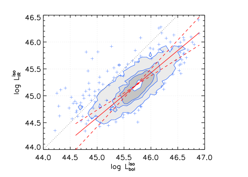
Figure 1: Comparison of bolometric luminosity $L_{\rm bol}^{\rm iso}$ and integrated IR luminosity $L_{\rm IR}^{\rm iso}$ as measured by WISE. Contour levels are at 10%, 50%, 68% and 95% of total source number (3965). The dotted line identifies equal luminosity. The solid line ($\log L_{\rm IR}^{\rm iso}\propto 0.83\log L_{\rm bol}^{\rm iso}$) is the bisector of the two least squares fitting (dashed) lines.

To provide a deeper insight on the disc–torus connection we select three subsamples according to $L_{\rm bol}^{\rm iso}$; we will refer to these subsamples with letters A, B, C. Tab. 2 lists the $\nu L_{\nu}$ IR luminosities in the four WISE bands for the whole sample and for the subsamples A, B, C, together with the average spectral indices. Tab. 3 reports the average and the standard deviation of $L_{\rm bol}^{\rm iso}$ and $L_{\rm IR}^{\rm iso}$ together with their ratio $R=L_{\rm IR}^{\rm iso}/L_{\rm bol}^{\rm iso}$ for the whole sample and for the A, B, C subsamples. For the latter, instead of the standard deviation of $L_{\rm bol}^{\rm iso}$, we give the logarithmic width of the considered luminosity bin. Note that sources in these subsamples account for only $\sim$1/3 of the entire sample. Dropping 2/3 of the sample was necessary to significantly separate the bolometric luminosity classes.

Table 3: Results of our analysis. Columns are: (1) sample; (2) number of sources in the sample; (3) mean bolometric luminosity in the sample; (4) width of luminosity bin (^a: value in the first row is the standard deviation); (5) mean and standard deviation of $L_{\rm IR}^{\rm iso}$ in the sample; (6) mean and standard deviation of parameter $R=L_{\rm IR}^{\rm iso}/L_{\rm bol}^{\rm iso}$; (7) range of covering factor (Eq. 10); (8) range of torus opening angles; (9) range of Type 2 to Type 1 AGN count ratio (#2/#1). All means and standard deviations are computed using logarithmic values.

Sample	N src.	log $L_{\rm bol}^{\rm iso}$	log $\Delta L_{\rm bol}^{\rm iso}$	log $L_{\rm IR}^{\rm iso}$	$R$	Cov. factor	$\theta_{\rm T}$	$\#2/\#1$
Whole	3965	45.72	0.33a	45.18$\pm$0.27	$0.29_{-0.11}^{+0.18}$	0.54–0.70	57–46	1.2–2.3
A	408	45.55	0.10	45.05$\pm$0.16	$0.31_{-0.10}^{+0.14}$	0.56–0.74	56–42	1.3–2.8
B	569	45.80	0.10	45.22$\pm$0.16	$0.26_{-0.08}^{+0.12}$	0.51–0.66	59–49	1.0–1.9
C	389	46.05	0.14	45.40$\pm$0.16	$0.22_{-0.07}^{+0.10}$	0.47–0.60	62–53	0.9–1.5

3.1 Consistency with broad emission lines

The estimates given above do not take into account that the observed optical continuum can include different components, besides the disc emission. As a consistency check, we use an alternative method to derive the disc (bolometric) luminosity, by using the luminosities of the H$\beta$ and the MgII broad lines, always present in the SDSS spectra in our redshift selection. For radiatively efficient discs, indeed, the overall luminosity of the broad line region (BLR), $L_{\rm BLR}$, is a proxy of the disc luminosity $L_{\rm bol}$, since on average $L_{\rm BLR}\sim\gamma L_{\rm bol}$, where the factor $\gamma$ is directly connected to the BLR covering factor (see e.g. Baldwin & Netzer 1978; Smith et al. 1981). In turn, $L_{\rm d}$ should be equal to $L_{\rm bol}$ (real, not isotropically equivalent). Estimates of $\gamma$ lie in quite large ranges, historically between 0.002 and 0.35 (according to Baldwin & Netzer), but preferentially $<0.15$ (Smith et al. 1981). Typically, an average value $\gamma\sim 0.05-0.1$ is assumed. $L_{\rm BLR}$ can be calculated from individual broad line luminosities, as in Celotti et al. (1997). Specifically, setting the Ly$\alpha$ flux contribution to 100, the relative weights of the H$\alpha$, H$\beta$, MgII and CIV broad lines are 77, 22, 34 and 63, respectively (Francis et al. 1991). The total broad line flux is fixed at 555.8. Since all our sources have measured H$\beta$ and MgII line luminosity, we average for each object the estimates of $L_{\rm BLR}$:

$$L_{\rm BLR}={1\over 2}\left[\frac{555.8}{22}L({\rm H}\beta)+\frac{555.8}{34}L({\rm MgII})\right]$$ (4)

A good agreement between the continuum–based and the BLR–based bolometric luminosities is obtained using $L^{\rm iso}_{\rm bol}=L_{\rm BLR}/0.041$. This value is found for sources in the highest luminosity subsample (C), for which we do not have spurious contributions from components other than the disc (e.g. host galaxy). Fig. 2 shows the histogram of the ratio $R$ for all sources (green solid line).

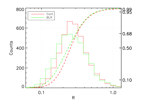
Figure 2: Histogram of $R$, as computed using integrated IR luminosity $L_{\rm IR}^{\rm iso}$ and both the continuum–based (red solid line) and BLR–based (green solid line) bolometric luminosities. Dashed lines show the cumulative fraction (values on right axis).

This histogram not only has the same average of the distribution of $R$ based on the 3000 Å luminosity (which is expected, given our assumptions), but the two distributions are similar for all $R$, implying that broad lines are a good proxy to compute the total disc luminosity, and that our estimates of $R$ are reliable.

4 The covering factor of the torus

Consider the simplest case of a doughnut–shaped torus with opening angle $\theta_{\rm T}$, as measured from the symmetry axis. The covering factor $c$ is defined as:

$$c=\frac{\Omega_{\rm T}}{4\pi}={2\times 2\pi\int_{\theta_{\rm T}}^{\pi/2}\sin\theta d\theta\over 4\pi}=\cos\theta_{\rm T}$$ (5)

We must relate $c$ to the observed ratio $R$, accounting for the anisotropy of disc and torus emission. Since the emission of geometrically thin discs follows a $\cos\theta$ pattern, for a given viewing angle $\theta_{\rm v}$ (calculated from the disc axis) the ratio between the real disc luminosity $L_{\rm bol}$ and the isotropic estimate $L_{\rm bol}^{\rm iso}$ is:

$${L_{\rm bol}\over L_{\rm bol}^{\rm iso}}={2\times 2\pi\int^{\pi/2}_{0}\cos\theta\sin\theta d\theta\over 4\pi\cos\theta_{\rm v}}={1\over 2\cos\theta_{\rm v}}$$ (6)

The ratio is smaller than unity for $\theta_{\rm v}<60^{\circ}$, thus for Type 1 AGN we likely have $L_{\rm bol}<L_{\rm bol}^{\rm iso}$. We are not able to determine $\cos\theta_{\rm v}$ for each source, but we can safely assert that $0\leq\theta_{\rm v}\leq\theta_{\rm T}$, since we are dealing with Type 1 AGN. Therefore a reasonable estimate is:

$$\cos\theta_{\rm v}\sim\langle\cos\theta\rangle_{0-\theta_{\rm T}}={\int_{0}^{\theta_{\rm T}}\cos\theta\sin\theta d\theta\over\int_{0}^{\theta_{\rm T}}\sin\theta d\theta}={1+\cos\theta_{\rm T}\over 2}$$ (7)

A relation similar to Eq. 6 for the torus luminosity ($L_{\rm T}=L_{\rm IR}$) is currently unknown. However, we can reasonably state that

$${L_{\rm bol}\over L_{\rm bol}^{\rm iso}}<{L_{\rm T}\over L_{\rm T}^{\rm iso}}<1$$ (8)

The lower limit corresponds to a thin disc–shaped emitting torus, the upper limit to an isotropic emitting torus. Both limits are rather unrealistic: the torus is expected to show a lower degree of anisotropy than the disc since we are able to detect radiation emitted from the side (i.e. Type 2 AGN); also, the torus is hardly an isotropic emitter since IR signatures are different in Type 1 and 2 AGN (Calderone et al., in prep.). The above limits should then bracket the real case. The amount of disc radiation intercepted (and re–processed) by the torus is:

$${L_{\rm T}\over L_{\rm bol}}={\int^{\pi/2}_{\theta_{\rm T}}\cos\theta\sin\theta d\theta\over\int^{\pi/2}_{0}\cos\theta\sin\theta d\theta}=\cos^{2}\theta_{\rm T}$$ (9)

Rearranging the previous equations, we find a relation between the observable parameter $R=L_{\rm IR}^{\rm iso}/L_{\rm bol}^{\rm iso}$ and the covering factor $c$:

$$\frac{c^{2}}{1+c}<R<c^{2}$$ (10)

This relation can be inverted to find the allowed range of $c$ and $\theta_{\rm T}$, given a value of the observable parameter $R$. Finally, the covering factor $c$ can be used to estimate the count ratio between Type 1 and Type 2 AGN:

$$c=\frac{\Omega_{\rm T}}{4\pi}=\frac{\#2}{\#1+\#2}\hskip 8.5359pt\Rightarrow\hskip 8.5359pt\frac{\#2}{\#1}=\frac{c}{1-c}$$ (11)

The last three columns of Tab. 3 report the value of $c$, $\theta_{\rm T}$ and #2/#1 corresponding to the observed values of $R$ in all discussed samples.

5 Discussion and conclusions

The main result of our work is the determination of the average covering factor of the torus using a very large data set. The observed fraction of IR to bolometric, isotropically equivalent optical luminosity is about 30%. This implies that the obscuring torus covering factor is in the range 0.5–0.7 and that the opening angle $\theta_{\rm T}$ is 40^∘– 60^∘. On average, our sources emit in the IR a similar fraction of their bolometric luminosities ($\sim 1/3$). For each Type 1 AGN, there should be between 1 and 3 Type 2 sources. If there is a broad distribution of covering factors (as suggested by Elitzur, 2012) our Type 1 sample may be drawn preferentially from the lower end of the distribution. In this case our estimate of #2/#1 ratio is a lower limit. The very basic prediction of the unified model that the torus re–processes a given amount of disc luminosity is verified (Fig. 1 and Fig. 2). The dispersion of this fraction is remarkably small, being at most a factor of 2. The broad–band spectral energy distribution (SED) from IR to near–UV are expected to be quite similar among Type 1 AGN. A hint of the “receding torus” hypothesis is found in Fig. 1, with $\log L_{\rm IR}^{\rm iso}\propto 0.83\log L_{\rm bol}^{\rm iso}$. In Fig. 3 we show both data and model for a prototypical broad–band SED, in the three luminosity classes considered above (coded with colors). For each subsample we also compute a composite spectrum using SDSS spectra.

Figure 3: The disc–torus connection. AGN in our sample were divided in three subsamples according to their bolometric luminosity (see Tab. 3), and associated to black, red and blue color respectively. The logarithmic mean and standard deviation of IR luminosities in each subsample are computed using data from WISE, and displayed as filled circles and error bars (points are slightly displaced for a clearer view). Composite optical/NUV spectra (solid color–coded lines) are computed as follows: SDSS spectra are transformed to rest–frame and de–reddened using Schlegel et al. (1998) and Pei (1992). The spectra are then rebinned to a common wavelength grid and a composite spectrum is computed as the geometric mean. The gray shades indicate the 68% level dispersion. Standard Shakura & Sunyaev (1973) accretion disc spectra fitting the composite spectra are shown with dashed lines. The disc–torus connection is clearly visible in this figure, in which the torus luminosity in all four WISE bands follows the trend in accretion disc bolometric luminosity. Discrepancies between the composite spectrum in the lower luminosity subsamples (black and red) and the accretion disc spectrum may be due to the contribution of host galaxy starlight (Vanden Berk et al. 2011). The yellow solid line shows the sum of the accretion disc spectrum (black dashed line) and the elliptical galaxy template from Mannucci et al. (2001) with a bolometric luminosity of log($L_{\rm host}$/erg s^-1) $\sim$ 44.3. The IR points may be modeled as sum (solid line) of at least two black bodies with temperatures 308 K and 1440 K (dot–dashed lines), and luminosities log($L_{\rm torus,BB}$/erg s^-1) = 45.00 and 44.91 respectively.

At IR wavelengths the torus emission dominates. Spectral indices between the four WISE bands are very similar for different overall luminosities (Tab. 2). Despite the rather poor coverage, it appears that the IR emission is structured with at least two broad bumps. Such features are easily modeled by the superposition of two black bodies with temperatures of $\sim$300 K and $\sim$1500 K respectively. A naïve interpretation is to consider the hotter one as emitted from the hot part of the torus facing the disc, at the dust sublimation temperature. The colder one would come from the cooler outer side of the torus. This should be the region visible also in Type 2 AGN.

The underlying optical continua are well described by a standard Shakura & Sunyaev (1973) accretion disc spectrum. The dashed lines in Fig. 3 are the models of three accretion discs having the same bolometric luminosity as the spectra in the subsample, and masses $1.7\times 10^{8}$, $2.3\times 10^{8}$ and $3.4\times 10^{8}$ M_☉ respectively, grossly in agreement with the (virial) masses calculated in S11. The WISE data points (in $\nu L_{\nu}$) lie a factor $\sim$3 below the disc peaks (at log($\nu$/Hz)$\sim$15.5). This factor corresponds to the value $\sim$1/3 found in Tab. 3 and Fig. 2. The composite spectra follow closely the accretion disc continuum in all but the lowest luminosity subsample, in which some other component is present at frequencies below log($\nu$/Hz)$<$14.9. This further component may be the starlight contribution from host galaxy (Vanden Berk et al. 2011), as shown by the yellow line which is the sum of the accretion disc spectrum and an appropriately scaled template for an elliptical (quiescent) galaxy from Mannucci et al. (2001). At higher luminosity subsamples, the contribution from galaxy becomes relatively less important.

References

- [] Antonucci R. & Miller J., 1985, ApJ, 297, 621
- [] Arshakian, T. G., 2005, A&A, 436, 817A
- [] Baldwin J.A. & Netzer H., 1978, ApJ, 226, 1
- [] Becker R.H., White R.L. & Helfand D.J., 1995, ApJ, 450, 559
- [] Celotti A., Padovani P. & Ghisellini G., 1997, MNRAS, 286, 415
- [] Chiaberge M., Capetti A & Celotti A., 1999, A&A, 349, 77
- [] Comastri A., Setti G., Zamorani G. & Hasinger G., 1995, A&A, 296, 1
- [] Elitzur M. & Shlosman I., 2006, ApJ, 648, L101
- [] Elitzur M., 2012, ApJ, 747L, 33
- [] Elvis M., Wilkes B.J., McDowell J.C. et al., 1994, ApJS, 95, 1
- [] Elvis M., 2000, ApJ, 545, 63
- [] Francis P.J., Hewett P.C., Foltz C.B., Chaffee F.H., Weymann R.J. & Morris S.L., 1991, ApJ, 373, 465
- [] Ghisellini G., Haardt F. & Matt G., 1994, MNRAS, 267, 743
- [] Gilli R., Comastri A. & Hasinger G., 2007, A&A, 463, 79
- [] Krolik J. & Begelman M.C., 1988, ApJ, 392, 702
- [] Krolik J., 1999, Active Galactive Nuclei, Princeton: Princeton Univ. Press
- [] Landt H., Elvis M., Ward M., Bentz M.C., Korista K.T. & Karovska M., 2011, MNRAS, 414, 218
- [] Lawrence A., 1991, MNRAS, 252, 586
- [] Madau P., Ghisellini G., Fabian A.C. 1994, MNRAS, 270, L17
- [] Mannucci F., Basile F., Poggianti B. M., Cimatti A., Daddi E., Pozzetti L., Vanzi, L., 2001, MNRAS, 326, 745M
- [] Nenkova M., Sirocky M.M., Ivezic Z. & Elitzur M., 2008, ApJ, 658, 147
- [] Pei Y. C., 1992, ApJ, 395, 130
- [] Peterson B.M., 1997, Introduction to Active Galactic Nuclei, Cambridge Univ. Press
- [] Richards G.T., Lacy M., Storrie–Lombardi L.J. et al., 2006, ApJS, 166, 470
- [] Risaliti G., Elvis M. & Nicastro F., 2002, ApJ, 571, 234
- [] Robson I., 1996, Active Galactic Nuclei, John Wiley and Sons, Ltd. in assoc. with Praxis Publishing, Ltd.
- [] Schlegel D.–J., Finkbeiner D. P., Davis M., 1998, ApJ, 500, 525
- [] Schneider D. P., Richards, G. T., Hall P. B. et al., 2010, AJ, 139, 2360S
- [] Setti G., & Woltjer L., 1989, A&A, 224, L1
- [] Shakura N.I. & Sunjaev R.A., 1973, A&A, 24, 337
- [] Shen Y., Richards G.T., Strauss M.A. et al., 2011, ApJS, 194, 45, (S11)
- [] Simpson, C., 2005, MNRAS, 360, 565S
- [] Smith M.G., Carswell R.F., Whelan J.A.J et al., 1981, MNRAS, 195, 437
- [] Vanden Berk D. E. et al., 2001, AJ, 122, 549
- [] Wills B., 1999, in Quasars and Cosmology, ASP Conf. Ser., vol. 162, p. 101, Ed. G. Ferland and J. Baldwin
- [] Wright E.L., Eisenhardt P.R.M., Mainzer A.K. et al., 2010, AJ, 140, 1868
- [] York D.G., Adelman J., Anderson J.E., Jr. et al., 2000, AJ, 120, 1579